Implications
Results of this study show that in different New Zealand flocks, increasing levels of early prolificacy were associated with an erosion of ewe lifespan. These findings have value to support farmers’ culling decisions that will contribute to reach a better compromise between ewe prolificacy and longevity in the flock. They also offer insights for the incorporation of longevity in selection indices targeting an improvement in ewe lifetime performance.
Introduction
Over the last 15 years, the efficiency of New Zealand (NZ) sheep systems has been substantially improved through breeding schemes mainly focussed on growth and prolificacy (Young and Amer, Reference Young and Amer2009; Byrne et al., Reference Byrne, Ludemann, Amer and Young2012). However, it is also essential that ewes can live and produce in the flocks for a sufficient period to be economically efficient from a lifetime perspective (Conington et al., Reference Conington, Bishop, Grundy, Waterhouse and Simm2001). Accordingly, several studies have suggested that the inclusion of traits related to productive lifespan in breeding objectives would be beneficial (Borg et al., Reference Borg, Notter and Kott2009; McIntyre et al., Reference McIntyre, Newman, Young and McEwan2012). However these traits are not very heritable, sex-limited and expressed late in life, which currently limits their scope for genetic improvement (Lee et al., Reference Lee, Cullen, Newman, Dodds, McEwan and Shackell2015). Alternatively, traits expressed early in the productive life of ewes can be used as predictors of lifetime performance (Lee and Atkins, Reference Lee and Atkins1996). In particular Amer et al. (Reference Amer, Jopson, Cocks and Scarlet2007) have shown that a high level of early prolificacy can compromise subsequent litter outputs in ewes from NZ breeding flocks. Under pastoral grazing conditions, bearing a large litter is a well-recognized risk factor for ewe health and the neonatal survival of her lambs (Scales et al., Reference Scales, Burton and Moss1986). However, the potential long-term effects on ewes’ lifespans remain so far unexplored. Such effects might well exist, as suggested for instance by the reduced longevity of highly prolific sheep breeds of lowlands when they are transferred in hill pastures environments (Hohenboken and Clarke, Reference Hohenboken and Clarke1981). In the present study, longitudinal ewe data were collected in NZ flocks with contrasting feeding conditions. The objective was to investigate the influence of the flock environment on the relationship between ewes’ level of early prolificacy, as estimated by the number of lambs born in the first 2 years of productive life, and their subsequent survival in the flock.
Material and methods
Data
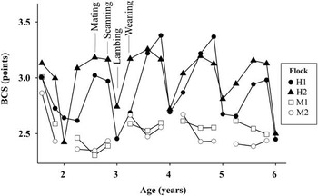
Data were provided by Sheep Improvement Ltd for four NZ breeders who had agreed for their data to be used in this study. Three of the flocks were located in the South Island and one in the North Island. Overall flock management was typical of NZ pasture fed-farming systems, although it was possible to split the four flocks into two moderately variable, and two highly variable flock environments based on observed body condition score (BCS) profiles across time points within the year. Seasonal variation in BCS is a management factor, whereby seasonal differences in pasture availability are managed through building body reserves in breeding ewes which are subsequently mobilized, rather than conserving surplus pasture for feeding, in periods of feed deficit. This is a management strategy common in harsher environments where topography or land quality make conservation and feeding of supplements impractical. Lambings took place on a yearly basis and were mostly concentrated from the end of August to mid-October so that the period of greatest nutritional requirements for breeding ewes matches the period of peak pasture growth. Most ewe replacements were first mated at 19 months so that their first lambing occurred at 2 years old, as ‘two-tooths’. About 3 months after mating, pregnancy was diagnosed with ultrasonic scanning. Ewes lambed outdoors and reared their lambs for about 3 months until weaning. Farmers systematically recorded the number of lamb born (NLB), the number of lamb weaned (NLW), and occasionally weighted the lambs at weaning. Moreover, at each of these events (except at lambing in certain flocks), the same technician assessed ewes BCS manually by feeling the level of muscling and fat deposition over and around the vertebrae in the loin region, and scoring this level on a five points scale with an half-point accuracy (Beef+Lamb New Zealand, 2013). Figure 1 shows the average BCS over time in the four flocks, and reflects the feeding strategy used on each property. The two flocks with a moderately variable environment (M1 and M2) maintained ewes at a relatively constant 2.5 BCS points, meaning that feed intake largely met feed demand throughout the year, either through pasture or supplementary feeding. The two flocks with a highly variable environment (H1 and H2) increased average BCS in spring and summer, and decreased in autumn and winter, corresponding to periods of high and low pasture quality and availability. The topography of the highly variable environments is such that breeders have limited options for conserving pasture to supplement ewes in periods of low availability. Therefore, ewes are fed to build body energy reserves when pasture is plentiful, and deplete these reserves when pasture is scarce. Stocking rate is managed so that ewes do not fall below an average BCS of 2.5 in winter, which coincides with the second and third trimesters of gestation.
Average lifetime changes in the body condition score (BCS scored on a 1 to 5 points scale) of ewes from four New Zealand flocks with contrasted feeding management. M1 and M2=flocks with a moderate environment; H1 and H2=flocks with a highly variable environment. Data were from 4003 ewes among those included in this study. Points=averages of available individual records.

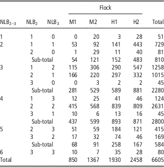
Data included in the study described the performance of 6605 ewes that lambed for the first time at 2 years old and that were mated the following year. These ewes were born between 1990 and 2011 on one of the two moderate environment farms (M1 and M2) or one of the two highly variable environment farms (H1 and H2). The distribution across farms was: M1 (13%), M2 (21%), H1 (29%) and H2 (37%) (Table 1). Most were Romney (in M1, M2 and H1) or composites of Texel and Romney breeds (in M2). Ewes that first lambed at 1 year old (as ‘hoggets’) were also present in the four flocks but they were excluded from the analysis as their number was too low to compare performance with ewes that first lambed at 2 years old (as ‘two-tooth ewes’). For each ewe, the sum of the NLB at 2 (NLB2) and 3 (NLB3) years old was calculated (NLB2–3) to estimate the level of early prolificacy. This variable NLB2–3 varied from one (i.e. single at first lambing and failure to lamb the following year) to six (triplets at both lambings). Ewes with NLB2 or NLB3 greater than three lambs were not considered. Although 2/3 of the ewes were in a highly variable flock environment, sample size for each level of NLB2–3 in flocks M1 and M2 was high enough to compare the effect of the level of early prolificacy between environments (Table 1). Most of the ewes (83% and 73% of those in the moderately and in the highly variable flock environment, respectively) had three or four lambs after 2 years of productive life, and mainly with combinations of singles and twins.
Distribution of the number of ewes in each New Zealand sheep flock of the study according to numbers of lambs born at 2 and 3 years old

NLB2–3=number of lambs born per ewe during the first two lambings at 2 and 3 years old; NLB2=number of lambs born at first lambing; NLB3=number of lambs born at second lambing; M1 and M2=flocks with a moderate environment; H1 and H2=flocks with a highly variable environment.
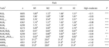
In addition to NLB2 and NLB3, others traits of early ewe productivity were recorded. The NLW at 2 (NLW2) and 3 (NLW3) years old were used to calculate the proportion of the litter that survives from birth to weaning (NLW/NLB), usually called the ewe rearing ability (e.g. Safari et al., Reference Safari, Fogarty and Gilmour2005). The average weaning weight (AWW) was also calculated as the average of the individual weaning weight of a ewe’s lambs at first lambing (AWW2), at second lambing (AWW3), and after both (AWW2–3). Numbers of observations for these different traits are detailed in Table 2.
Summary of average ewe production over the first two parities at 2 and 3 years old

M1 and M2=flocks with a moderate environment; H1 and H2=flocks with a highly variable environment; High–moderate=effect of the flock environment (considering the moderate environment as baseline) on each trait described ; NLB=number of lambs born par ewe, NLW=number of lambs weaned par ewe, NLW/NLB=proportion of the litter that survives from birth to weaning (i.e. ewe rearing ability), AWW=average weaning weight of the individual lamb in a litter.
Means within rows sharing a common character in their superscript are not significantly different (P>0.05) after correction for year effect in a logistic model and pairwise comparisons (Tukey’s test).
1 Subscripts 2 and 3 refer to the first and second parity (when the ewes where 2 and 3 years old), respectively. Subscript 2–3 refers to both parities.
Level of statistical significance denoted by asterisk: *P<0.05, **P<0.01, ***P<0.001.
Several measures of ewe longevity were considered in this study. The age at exit from the flock was assumed to be the age (in years) at which the last NLB measurement was recorded. Ewe stayability i|j was defined as a binary trait (0 or 1) that describes her survival to a specific age i given that she already lived until j years old. Measures of overall stayability i|3 could be established for the 6605 ewes with i varying from 4 to 10 years because all ewes considered for study survived until at least 3 years old. Measures of marginal stayability i|(i – 1) were also established to determine the rate of disappearance at a particular age. These last measures were missing for ewes that were removed from the flock at age i – 1 or before.
Statistical analysis
Binary traits of stayability and lamb survival were analysed by logistic regression using a generalized linear model with a binomial distribution and a logit-link function in R (GLM function in R 3.2.1; R Core Team, 2015). Others traits of ewes performance (NLB, NLW and AWW traits) were analysed by linear regression. The flock average effects with the SEM of all these traits were calculated in the model including ewe flock and year of birth as fixed effects. Thereby flock averages were adjusted for the long-term trends and the annual fluctuations on ewe performance recorded over the 21 years of available data. To investigate the effects of the level of ewes’ early prolificacy on their stayability, NLB2–3 was included either as a continuous or as categorical independent variable. In the first case, the aim was to analyse the shape of the relationship between stayability traits and NLB2–3. For this, the following GLM was used:
 $$\eqalignno{{\rm log}\left( {{{y_{{ijk}} } \over {1{\minus}y_{{ijk}} }}} \right){\rm {\,\equals\,}} & \mu {\rm {\plus}ENV}_{j} {\rm {\plus}YEAR}_{k} {\rm {\plus}}\beta _{{1j}} \left( {{\rm NLB}_{{{\rm 2{\minus}3}}} } \right)_{{ijk}} \cr &{\rm {\plus}}\beta _{{2j}} \left( {{\rm NLB}_{{{\rm 2{\minus}3}}} } \right)_{{ijk}}^{2} {\rm {\plus}}{\epsilon}_{{ijk}} ,$$
where y ijk is the stayability measure of ewe i, μ the overall mean effect, ENV j the effect of flock environment j (moderate v. highly variable), YEAR k the effect of ewe birth year k (from 1990 to 2011), β 1j and β 2j the linear and quadratic effects, respectively, of NLB2–3, and which depend on the flock environment j, ε ijk the residual effect. A positive effect of NLB2–3 on ewe stayability was expected as to some extent breeders prefer to keep prolific ewes in their flock and to cull the less prolific ones. However, inclusion of a quadratic effect of NLB2–3 also allowed a possible decline in ewe stayability with high levels of prolificacy to be detected. As β 1 and β 2 were positive and negative respectively in all cases, the value of NLB2–3 that maximizes ewe stayability (Optimal NLB2–3) could be calculated as follows:
 $${\rm Optimal}\,{\rm NLB}_{{2{\minus}3}} {\,\equals\,}{\minus}{{\beta _{1} } \over {2{\times}\beta _{2} }}$$
In addition to the prolificacy effects associated with NLB2–3, the effect of lamb survival between birth and weaning was investigated. This was done by adding to model (1) an effect β 3 of the total number of lambs dead after the first two parities (NLB2–3–NLW2–3) and its interaction with the flock environment. Simplification of model (1), and of its more complex version including the number of lambs dead, involved stepwise dropping of the least significant term and testing with a likelihood ratio test of comparison whether or not the removal of this term significantly improved the model goodness-of-fit.
In the case where NLB2–3 was included as a categorical variable in the logistic regression of stayability traits, the individual effects of each level of NLB2–3 were determined in each flock environment, and after correction for year effects. For this the logistic model of each stayability trait was fitted with the interaction ENV j ×(NLB2–3) m (with m varying from 1 to 6) plus the YEAR effect. The predicted average effects of the interaction together with their 95% confidence interval (CI) were computed with logit transformation. Differences in average stayability between flock environments were assessed at each level of NLB2–3 using Tukey’s test in the multcomp R-package (Hothorn et al., Reference Hothorn, Bretz and Westfall2008). To investigate whether or not the combinations of NLB2 and NLB3 that result in a same NLB2–3 (Table 1) have different effects on ewe stayability, the same procedure was used but replacing the interaction ENV j ×(NLB2–3) m by the interaction ENV j ×(NLB2) n ×(NLB3) o with n and o varying from 1 to 3 and denoting the litter size at 2 and 3 years, respectively (o=0 was ignored due to low sample size).
Finally, the effects of the level of early prolificacy on simultaneous ewes’ productivity (ewe rearing ability and AWW2–3) were also investigated as previously described for the stayability analysis, using NLB2–3 both as a continuous and as a categorical variable. A logistic model was used for the analysis of rearing ability whereas a linear model was used for AWW.
Results
Flock averages
Several differences in the level of ewe productivity were detected across flocks (Table 2). Flocks M1 and H2 have the greatest and the lowest level of productivity, respectively, in line with the difference in nutritional environments. In contrast, ewes’ performance in M2 was relatively low – close to H2 – and that of H1 was relatively high – close to M1. These latter variations, as well as those observed for AWW, were opposite to the expected environmental effects and were assumed to reflect genetic differences across flocks. The overlap in ewe performance across flock environments showed the possibility of reaching a relatively high production level in a highly variable environment.
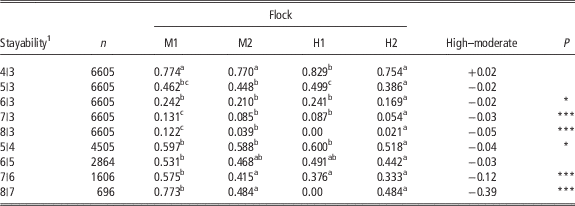
The above flock contrasts were partly observed for stayability measures (Table 3). For overall stayability to intermediate age (5|3 and 6|3), the flock environment effect was only reflected in the difference between M1 and H2. However, the effect became clearer between all flocks at latter ages (stayability 6|3, 7|3, and 8|3). In flock H1, no ewe remained more than 7 years in the flock, which might reflect a systemic culling decision (it is common practice that farmers tag their ewes with a different colour tag for each birth year, so that they can subsequently detect and separate those that reached a certain age, considered as a critical age in terms of risk to die on farm). Marginal stayability traits were less accurately determined than overall stayability traits, especially at old ages (stayability 6|5 and older ages), because of reduced sample size (Table 3). For these traits, the most significant differences (P<0.001) between flock environments were also expressed at late ages (from stayability 7|6), showing that the proportion of old ewes is greater in moderate than in highly variable flock environments.
Means of ewe stayability traits across the New Zeland flocks of the study

M1 and M2=flocks with a moderate environment; H1 and H2=flocks with a highly variable environment; High–Moderate=effect of the flock environment (considering the moderate environment as baseline) on each stayability trait described.
Means within rows sharing a common character in their superscript are not significantly different (P>0.05) after correction for year effect in a logistic model and pairwise comparisons (Tukey’s test).
1 Stayability i|j describes the probability of a ewe to survive in the flock until i years old, given that she already survived until j years old.
Level of statistical significance denoted by asterisk: *P<0.05, **P<0.01, ***P<0.001.
Stayability analysis
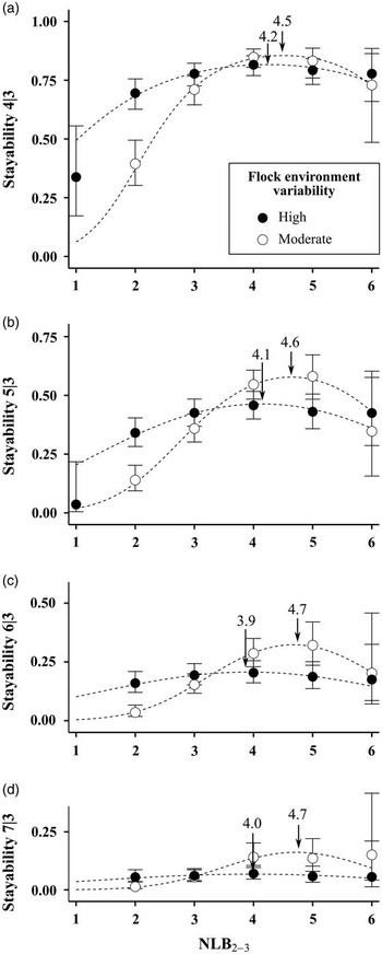
There was a curvilinear relationship between NLB2–3 and overall stayability traits in both flock environments (Figure 2). Ewes with low levels of prolificacy (NLB2–3⩽2 lambs) were more likely to exit the flock early than ewes with greater levels, but a too high level negatively affected ewes’ lifespan as well. The shape of the relationship was significantly different between flock environment for all the stability traits between 4|3 and 7|3 (Supplementary Table S1). First, low levels of early prolificacy were more detrimental in a moderate environment than in a highly variable environment. This was in line with a stronger breeder’s selection pressure on productivity in the moderate farm environment. Second, although the maximum level of stayability in the moderate flock environment was consistently superior to the level observed in the highly variable environment, the drop associated with high levels of NLB2–3 was also more pronounced. The magnitude of these two effects changed as stayability to latter ages was considered, which resulted in an increasing difference between the optimal NLB2–3 of each flock environment (Figure 2 and Supplementary Table S1).
Overall stayability of ewes according to the total number of lamb born during their first lambings at 2 and 3 years old (NLB2–3) in two contrasted New Zealand flock environments. Overall stayability 4|3 (a), 5|3 (b), 6|3 (c) and 7|3 (d) describes the probability that a ewe was present in the flock at 4, 5, 6 and 7 years old, respectively, given that she was present at 3 years old. Points=means (corrected for year effects) with bars representing the 95% confidence interval. Dashed lines=regression lines of a logistic model relating each stayability trait to NLB2–3 and NLB2 2–3 in both environments. Arrows=optimal NLB2–3

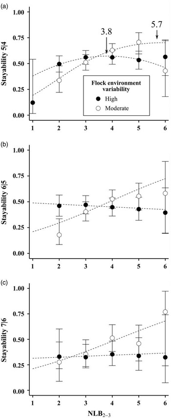
Effects of NLB2–3 on marginal stayability traits were less obvious than for overall stayability traits (Figure 3). Although NLB2–3 has a slight curvilinear effect on stayability 5|4, this effect disappeared (P>0.05) when only ewes living longer than 5 years were considered (stayability 6|5 and to older ages, Supplementary Table S2). Moreover in the highly variable environment, the stayability of these ewes was not affected at all by NLB2–3 when they were compared together (see β 1Highly variable in Supplementary Table S2). In the moderate flock environment, NLB2–3 had a positive effect on stayability, even among oldest ewes only (e.g. β 1Highly variable for stayability 7|6).
Marginal stayability traits of ewes according to the total number of lamb born during their first lambings at 2 and 3 years old (NLB2–3) in two contrasted New Zealand flock environments. Marginal stayability 5|4 (a), 6|5 (b) and 7|6 (c), described, respectively, the probability that a ewe was present in the flock at 5, 6 and 7 years old given that she was present at 4, 5 and 6 years old, respectively. Points=means (corrected for year effects) with bars representing the 95% confidence interval. Dashed lines=regression lines of a logistic model relating each stayability trait to NLB2–3 and NLB2 2–3 in both environments. Arrows=optimal NLB2–3 (when an effect of NLB2 2–3 was detected).

Inclusion of the number of lambs dead significantly improved the model that relates NLB2–3 to stayability traits. The total number of lambs dead during the first 2-year of productive life had a negative effect on stayability. For stayability 4|3, 5|3, 6|3, 7|3 and 8|3, β 3 was equal to −0.53 (Sx.y=0.04), −0.40 (Sx.y=0.04), −0.39 (Sx.y=0.05) and −0.34 (Sx.y=0.07), respectively, and did not differ significantly between flock environments. Thus, for instance the model predicts that when one lamb out of four died during early productive life, the ewe stayability 4|3 drops from 0.88 (CI=0.85 to 0.91) to 0.82 (CI=0.77 to 0.86) in the moderate environment, and from 0.86 (CI=0.83 to 0.89) to 0.79 (CI=0.74 to 0.83) in the highly variable environment. No statistical differences in stayability were detected between combinations of NLB2 and NLB3 resulting in a same level of NLB2–3 (P>0.80 for the five pairwise comparisons NLB2 v. NLB3; 1/2 v. 2/1, 1/3 v. 2/2, 1/3 v. 3/1, 2/2 v. 3/1 and 2/3 v. 3/2 in each environment).
Early productivity
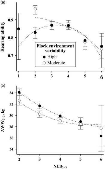
In the moderate flock environment, as it could be expected, ewe rearing ability over the first two parities tended to decrease with increasing levels of early prolificacy (Figure 4). In contrast, in the highly variable flock environment ewes had greater rearing ability at an intermediate level of prolificacy. Overall, the rearing ability of medium and high prolificacy ewes (NLB2–3⩾3) was unaffected by the environment whereas that of low prolificacy ewes (NLB2–3<3) was severely impaired, indicating a greater environmental sensitivity for low prolificacy ewes compared to medium and high prolificacy ewes. Accordingly, when including NLB2–3 as a continuous independent variable, the associated effects (β 1 and β 2) on lamb survival were only statistically different from zero in the highly variable environment (β 1Highly variable=1.00, Sy.x=0.15, P<0.001 and β 2Highly variable=−0.15, Sy.x=0.02, P<0.001), indicating an optimal NLB2–3 of 3.3 lambs with respect to rearing ability in the first two parities in a highly variable environment. However, as indicated in Figure 4, the curvature of the fitted curve was imposed by the concentration of data between NLB2–3=2 and NLB2–3=5. Smaller CI for the extreme values of NLB2–3 may have revealed a different shape.
Ewe rearing ability (a) and average weaning weight (b) of the lambs produced during the first lambings at 2 and 3 years old (AWW2–3) according to the corresponding number of lambs (NLB2–3) observed in two contrasting New Zealand flock environments. Ewe rearing ability was calculated as NLW2–3/NLB2–3 with NLW2–3 the number of lambs weaned among the NLB2–3 that were born. Points=means (corrected for year effects) with bars representing the 95% confidence interval. Dashed lines=regression lines of a logistic model relating the rearing ability or AWW2–3 to NLB2–3 and NLB2 2–3.

As expected, AWW2–3 decreased as NLB2–3 increased, however the decrease was stronger in the highly variable than in the moderate environment (Figure 5) with significant difference in β 2 (β 2Highly variable–β 2Moderate=−0.07/kg2, Sy.x=0.02, P<0.01, with β 1=−3.77/kg, Sy.x=0.49, P<0.001 in both environments). This model was significantly better than a model without the interactions between the flock environment and NLB2–3, and NLB2 2–3 (χ 2=126, df=1, P<0.01).
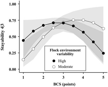
Predicted ewe stayability to 4 years old (stayability 4|3) according to the body condition score (BCS, scored on 1 to 5 points scale) when the ewe weaned her lambs at 3 years old. Solid lines and points=predicted means (corrected for year effects). Shaded areas=95% confidence interval of prediction.

Potential effects of body condition score
To explore further the relationship between the flock environment and ewes’ stayability, the influence of BCS at weaning of 3-year-old ewes (at the end of the early productive period) on stayability 4|3 was explored. A logistic model similar to model (1) but replacing NLB2–3 by BCS at weaning at 3 years old was fitted for 693 ewes which had BCS records; predicted values and their CI are reported (Figure 5). This model, once it has been simplified, revealed a positive effect of BCS on stayability (β 1Moderate=2.92, P<0.01, β 1Highly variable=2.13, P<0.05), showing that ewes too lean after the first two lambings are more likely to exit the flock than ewes with moderate BCS. This effect only tended to be different between flock environments (P=0.07). In addition BCS had a curvilinear effect on stayability independent from the flock environment (β 2=−0.39, P<0.01) which showed that ewes relatively too fat at weaning at age 3 were less likely to survive. Interestingly, including NLB2–3 as another predictor of stayability 4|3 (in addition to BCS and BCS2) did not improve the model (χ 2=0.75, df=1, P=0.39).
Discussion
For more than 30 years, research on genetic improvement of sheep litter size has addressed the existence of various optimum levels of prolificacy for different production environments (Bradford, Reference Bradford1985). Although the different optima were initially highlighted for contrasting situations (e.g. extensive v. intensive production systems), the optimum litter size can also vary between similar production systems that share different management characteristics, as it is the case for NZ pasture-based systems (Amer et al., Reference Amer, McEwan, Dodds and Davis1999). In all cases, the desired level of prolificacy is generally determined in relation to lamb performance, with little regard for ewe performance. This maternal aspect raises concerns for the production efficiency of sheep flocks, because an erosion of productive longevity is considered to reduce lifetime efficiency. In this study, the objective was to investigate the relationship between the level of ewes’ prolificacy early in their productive lives and their latter stayability in two contrasting NZ flock environments. The results showed that in a highly variable flock environment the level of early performance of ewes was more detrimental to their lifespan than in a moderate flock environment. This might explain why many sheep farms on highly variable environments have a preference for genetic strains of sheep with more moderate genetic potential for prolificacy. This leads on to the general consensus that it is time to start tempering the amount of selection emphasis placed on prolificacy in the NZ national breeding objective.
Different flock factors, such as breed composition or culling management, may have confounded the observed differences in ewe stayability between flock environments so this should be addressed as a potential limitation in the present study. First, some variation in weaning weight was apparently related to the breed differences, but this could also extend to others aspects of performance such as ewe stayability (e.g. Hohenboken and Clarke, Reference Hohenboken and Clarke1981). However, accounting for the heterogeneity in breed composition among flock environments in a supplementary analysis did not revealed any substantial influence on the observed difference in ewe stayability (Supplementary Table S3). Second, as our data comes from industry flocks with all the complexity of differing management from year to year, differences in ewe stayability may also have been caused by a number of non-biological factors related to farm management (e.g. preferential feeding of multiple-bearing ewes after scanning to improve ewes’ body condition and increase the survival rate of their lambs, preferential feeding of ewes with low body condition prior to mating). This could introduce biases into the analyses but in our view, the large amount of data included allowed to obtain reasonable estimates of differences between environments without factoring the management variants. The most important bias could have been caused by differences in culling management. In particular, it may be the case that ewes with low levels of prolificacy were able to live longer than observed, but were culled precociously by breeders due to their low production (Amer et al., Reference Amer, Jopson, Cocks and Scarlet2007). Indeed, ewes from ram breeder flocks are commonly culled on their performance records or estimated breeding values, or both, for the purpose of increasing genetic gain and reducing the generation interval (Lee et al., Reference Lee, Cullen, Newman, Dodds, McEwan and Shackell2015). This effect should mostly occur early in productive life and accordingly in this study, ewes which had two lambs or less at 2 and 3 years old were less likely to be presented for a third breeding event compared to their more productive counterparts. In addition, the ewes’ ability to express their genetic potential for prolificacy clearly depends on nutritional factors (Scaramuzzi and Radford, Reference Scaramuzzi and Radford1983) so not surprisingly breeders seemed to put more selective pressure on ewe prolificacy in a moderate than in a highly variable flock environment. Knowledge of the culling reasons would be helpful to further disentangle the influence of biological and management factors on ewes’ lifespan in the flocks (Mekkawy et al., Reference Mekkawy, Roehe, Lewis, Davies, Bünger, Simm and Haresign2009). Still, in the context of this study, several findings suggest that the lifetime performance of ewes with a low level of prolificacy early in productive life tends to be inherently inferior to that of others ewes. First, the finding that their rearing ability was highly sensitive to the environment indicates that these low prolific ewes tend to strongly prioritize their own survival and maintenance over that of their lamb. In contrast, the rearing ability of more prolific ewes (NLB2–3⩾3) was not different between flock environments, in line with the results of feeding experiments with twin- and triplet bearing ewes in NZ grazing conditions (Morris and Kenyon, Reference Morris and Kenyon2004). Further, results suggest that the poor rearing ability of low prolificacy ewes may well have been the reason for their precocious culling in the highly variable flock environment. In particular, ewes that fail to rear a lamb during their first parity tend to repeatedly exhibit a reduced survival of their lamb and a lower fertility for the subsequent cycles (Lee and Atkins, Reference Lee and Atkins1996; Amer et al., Reference Amer, Sise, Jopson and Bray2009). Indeed, Borg et al. (Reference Borg, Notter and Kott2009) have shown a positive association between the ewe’s ability to provide a superior maternal care and their stayability to 5 years of age. Second, the observation that ewes with low prolificacy had a reduced marginal stayability to 6 years and more, only in a moderate environment, suggests that these ewes were not limited by the amount of feed resources available in the flock environment but rather by their drive to acquire and use these resources. This is supported by a positive genetic correlation (r=0.27) between ewe prolificacy and her adult BW (Safari et al., Reference Safari, Fogarty and Gilmour2005) – which is reasonably well associated with the food intake capacity. Other supporting evidence comes from ecological studies showing that the phenotypically heaviest ewes are generally those with the longest lifespan in wild populations (Gaillard et al., Reference Gaillard, Festa-Bianchet, Delorme and Jorgenson2000).
With regard to high prolificacy ewes, our results indicate that their survival at 4 years old and more can be impaired by a temporary underfeeding during early productive life. Such a phenomenon is widely shown in the wild (Nussey et al., Reference Nussey, Froy, Lemaitre, Gaillard and Austad2013) and is generally explained by an accelerated deterioration of the reproductive or survival functions, or both, with age for animals that grew quickly and reproduced precociously (Lemaître et al., Reference Lemaître, Berger, Bonenfant, Douhard, Gamelon, Plard, Gaillard, Lyon and De Biome2015). Although domesticated sheep breeds may show an earlier loss of the reproductive function than wild breeds (Mysterud et al., Reference Mysterud, Steinheim, Yoccoz, Holand and Stenseth2002), the present analysis of marginal stayability (4|3 and 5|4) suggests that the negative effects of NLB2–3 on ewes’ lifespans occurred shortly after the early reproductive effort, probably before the onset of reproductive senescence. Therefore the carry-over effects of a high litter size at one lambing on subsequent litter outputs (Amer et al., Reference Amer, Jopson, Cocks and Scarlet2007) may also affect ewe survival. A possible mediation of this effect through ewe lifetime might be the excessive loss of body reserves, as in this study and elsewhere (Annett et al., Reference Annett, Carson, Dawson, Irwin, Gordon and Kilpatrick2011) a low body condition score at weaning is associated with a low stayability. Alternatively the adverse effects of a high level of early prolificacy on the subsequent ewes’ survival may primarily reflect a mismatch between the ewes’ genetic potential for growth and reproduction and their nutritional environment. In support of this hypothesis, Borg et al. (Reference Borg, Notter and Kott2009) showed negative genetic correlations between several growth traits and ewe stayability. Ewes generally reach their mature body size after 4 or 5 years so a high reproductive effort in early life may hinder their full body development and ultimately shorten lifespan. The breeding of ewes early in life as hoggets can lead to a reduced mature BW, however no effects of longevity have been detected yet (Kenyon et al., Reference Kenyon, Thompson and Morris2014). Although breeding ewes to first lamb at 1 year of age is currently advocated in New Zealand as an efficient management option to increase lifetime productivity, results from this study suggest that further investigation in contrasting flock environments may lead to different conclusions.
This study may have implications for the NZ sheep industry, which has achieved a substantial increase in genetic potential for ewe prolificacy (Young and Amer, Reference Young and Amer2009) and simultaneously a shift in the land used for sheep production with an increasing proportion of hill country pastures (Young and Thomson, Reference Young and Thomson2014). In this context, identifying robust ewes – that can sustain their production despite the large changes in feed quantity and quality – will be crucial in NZ sheep flocks. In the long-term robustness is likely to be partly reflected in ewe stayability whereas in the medium term the change in body condition throughout the productive cycles has been proposed as a potential indicator (Young and Thomson, Reference Young and Thomson2014). Still the question remains as to whether robust ewes rely heavily on their body reserves to cope with periods of underfeeding or if they tend to maintain a constant level of body condition. This latter case was circumstantially supported in this study. Similarly, Rauw et al. (Reference Rauw, Thain, Teglas, Wuliji, Sandstrom and Gomez-Raya2010) showed that ewes with the smallest loss of BW during their productive cycle in very harsh grazing conditions (cold desert Nevada) are the most adapted. In addition Rose et al. (Reference Rose, Kause, Mulder, van der Werf, Thompson, Ferguson and van Arendonk2013) found that the loss of ewe BW during nutritional restriction can be included in breeding programmes. Future research on the genetic correlation between ewe BW loss and lifespan would be instructive to explore the effects of including these traits in genetic evaluation as a means of improving lifetime efficiency in NZ flocks.
Acknowledgements
The authors are grateful to Sheep Improvement Ltd for providing access to the data used in this study. They are also very grateful to the four breeders who agreed to make their data available.
Supplementary material
To view supplementary material for this article, please visit http://dx.doi.org/10.1017/S1751731116001002