

1 Introduction
The purpose of this study is to present a comprehensive account of the nonlinear stability analysis of plane Poiseuille and plane Couette flows in the presence of an unstable temperature gradient. In contrast to the well-known Rayleigh–Bénard–Poiseuille and Rayleigh–Bénard–Couette systems, where the temperature gradient stems from the externally imposed thermal boundary conditions, here, the temperature gradient is induced by viscous dissipation which acts as an internal heat generation.
In the absence of a thermal gradient, plane Poiseuille and plane Couette isothermal flows have been extensively investigated in the past as prototypes of shear flows. Their linear and nonlinear behaviours are driven purely by inertia, the impact of which can be measured with a single dimensionless parameter, the Reynolds number  $Re$. In summary, Orszag (Reference Orszag1971) showed that the plane Poiseuille flow becomes linearly unstable at
 $Re=5772$ (
 $Re$ is based on the channel half-width and the centreline velocity). In the case of weak disturbances in a channel of finite length, the linear threshold
 $Re=5772$ was confirmed qualitatively by the experiments conducted by Nishioka, Iida & Ichikawa (Reference Nishioka, Iida and Ichikawa1975). For high intensity disturbances in the inlet flow, Nishioka & Asai (Reference Nishioka and Asai1985) concluded from their experiments that the minimum transition Reynolds number is approximately
 $Re=1000$. Numerical simulations performed by Orszag & Patera (Reference Orszag and Patera1980) showed that finite-amplitude two-dimensional waves become unstable to infinitesimally small three-dimensional perturbations for
 $Re>1000$. In the case of plane Couette flow, Romanov (Reference Romanov1973) showed that this flow is linearly stable for all Reynolds numbers. In numerical simulations (Dauchot & Daviaud Reference Dauchot and Daviaud1995) and laboratory experiments (Tillmarki & Alfredsson Reference Tillmarki and Alfredsson1992), the lowest Reynolds numbers at which turbulence can be sustained has been shown to be between 300 and 400.
On the other hand, a vast literature exists on Rayleigh–Bénard–Poiseuille/Couette systems and the interested reader is referred to Nicolas (Reference Nicolas2002) for a comprehensive review. These systems have recently attracted an increased interest as simple configurations representing open systems to study the transition from convective to absolute instability in Newtonian fluids (Carrière & Monkewitz Reference Carrière and Monkewitz1999; Martinand, Carrière & Monkewitz Reference Martinand, Carrière and Monkewitz2006; Ouarzazi et al. Reference Ouarzazi, Mejni, Delache and Labrosse2008), in binary fluid mixtures (Hu, Ben Hadid & Henry Reference Hu, Ben Hadid and Henry2007) and in viscoelastic fluids (Hirata et al. Reference Hirata, de B. Alves, Delenda and Ouarzazi2015; de B. Alves, Hirata & Ouarzazi Reference de B. Alves, Hirata and Ouarzazi2016). Transient growth mechanisms have also been investigated in a Rayleigh–Bénard–Poiseuille system by Biau & Bottaro (Reference Biau and Bottaro2004) in the case of a stable stratification. In the presence of unstable stratification due to buoyancy forces, transient growth was analysed in Rayleigh–Bénard–Poiseuille/Couette systems by Jerome, Chomaz & Huerre (Reference Jerome, Chomaz and Huerre2012).
In the above brief review, the Poiseuille/Couette flows are considered isothermal or subjected to an external temperature gradient. Recent studies have shown that viscous dissipation can induce thermoconvective instabilities even without external forcing. A bibliographic survey on thermal instabilities induced by viscous dissipation, either in a fluid or in a fluid-saturated porous medium, can be found in Barletta (Reference Barletta2015). The buoyancy-induced instabilities caused by viscous dissipation in plane Couette flow (PCF) and plane Poiseuille flow (PPF) were studied respectively by Barletta & Nield (Reference Barletta and Nield2010) and Barletta, Celli & Nield (Reference Barletta, Celli and Nield2011). The authors considered an adiabatic lower horizontal wall and an upper isothermal wall. With such boundary conditions, no external thermal forcing is prescribed, and the temperature gradient of the basic flow is only a consequence of the flow rate, through the volumetric heating induced by viscous dissipation.
Barletta & Nield (Reference Barletta and Nield2010) proved that the longitudinal rolls superposed on the PCF are the most unstable normal modes. These authors showed that the order parameter for the onset of convective instability is given by the product  $Ge\,Pe^{2}$, where
 $Ge$ is the Gebhart number and
 $Pe$ is the Péclet number. The critical value of
 $Ge\,Pe^{2}$ is given by 2772.27 (Barletta & Nield Reference Barletta and Nield2010). A similar analysis of the PPF was developed by Barletta et al. (Reference Barletta, Celli and Nield2011). Also in this case, the longitudinal rolls turned out to be the most unstable normal modes with a critical value of
 $Ge\,Pe^{2}$ given by 221.2619. More precisely, those critical values of
 $Ge\,Pe^{2}$ were evaluated in both cases by assuming an infinitely large Prandtl number,
 $Pr$. This limit is a sensible one given that the sole cause of the instability is the viscous dissipation. In fact, Barletta et al. (Reference Barletta, Celli and Nield2011) proved that the critical value of
 $Ge\,Pe^{2}$ decreases with
 $Pr$ and attains its minimum when
 $Pr\rightarrow \infty$.
For instability induced by viscous dissipation, inertia is no longer the sole source of nonlinearity. Nonlinear thermal advection and the nonlinear contribution of viscous dissipation interact in a non-trivial way, even at low  $Re$. Therefore, the impact of these nonlinearities is examined in the framework of a weakly nonlinear stability analysis for the instability caused by viscous dissipation both in the PPF and PCF configurations. Our aim is to determine the nature of the bifurcation (supercritical/subcritical) and to report a quantitative analysis of the equilibrium disturbance amplitude and the average heat transfer beyond the bifurcation point.
The plan of this article is as follows. In § 2, the governing equations, the basic state and the formulation of its linear stability are presented. A weakly nonlinear analysis is performed in § 3 with the derivation of the amplitude equation. Results on the nature of bifurcations, the equilibrium amplitude of finite disturbances and the average heat transfer are presented in § 4. A conclusion is given in § 5.
2 Governing equations, basic state and dominant modal instability
Let us consider PPF or PCF between two horizontal impermeable walls, which are set at a distance  $h$ apart. For PCF, the top wall moves at a constant velocity, while the lower wall is supposed at rest. For both configurations, the upper wall is kept at a constant temperature
 $T_{1}$, while the lower wall is adiabatic. We assume that the Oberbeck–Boussinesq approximation holds and we take into account viscous dissipation.
The governing equations are non-dimensionalized with the use of the following non-dimensional quantities:
 $$\begin{eqnarray}\displaystyle (x,y,z)=\frac{(x^{\ast },y^{\ast },z^{\ast })}{h},\quad t=\frac{\unicode[STIX]{x1D705}}{h^{2}}t^{\ast },\quad \boldsymbol{u}=\frac{h}{\unicode[STIX]{x1D705}}\boldsymbol{u}^{\ast },\quad P=\frac{h^{2}}{\unicode[STIX]{x1D707}\unicode[STIX]{x1D705}}P^{\ast },\quad T=\frac{(T^{\ast }-T_{1})\unicode[STIX]{x1D6FD}gh^{3}}{\unicode[STIX]{x1D708}\unicode[STIX]{x1D705}}, & & \displaystyle \nonumber\end{eqnarray}$$
where  $\boldsymbol{u}^{\ast }=(u^{\ast },v^{\ast },w^{\ast })$,
 $T^{\ast }$ and
 $P^{\ast }$ are the dimensional velocity vector, temperature and pressure, respectively. While
 $\unicode[STIX]{x1D705}$ is the thermal diffusivity,
 $\unicode[STIX]{x1D70C}_{0}$ is the reference mass density,
 $\unicode[STIX]{x1D708}$ is the kinematic viscosity,
 $\unicode[STIX]{x1D707}$ is the dynamic viscosity,
 $\unicode[STIX]{x1D6FD}$ is the thermal expansion coefficient of the fluid and
 $g$ is the modulus of the gravitational acceleration. The dimensionless governing equations for continuity, momentum and energy can be written as (Barletta et al. Reference Barletta, Celli and Nield2011)
 $$\begin{eqnarray}\displaystyle & \displaystyle \unicode[STIX]{x1D735}\boldsymbol{\cdot }\boldsymbol{u}=0, & \displaystyle\end{eqnarray}$$
 $$\begin{eqnarray}\displaystyle & \displaystyle \frac{\unicode[STIX]{x2202}\boldsymbol{u}}{\unicode[STIX]{x2202}t}+(\boldsymbol{u}\boldsymbol{\cdot }\unicode[STIX]{x1D735})\boldsymbol{u}=Pr(-\unicode[STIX]{x1D735}P+T\boldsymbol{e}_{z}+\unicode[STIX]{x1D735}^{2}\boldsymbol{u}), & \displaystyle\end{eqnarray}$$
 $$\begin{eqnarray}\displaystyle & \displaystyle \frac{\unicode[STIX]{x2202}T}{\unicode[STIX]{x2202}t}+\boldsymbol{u}\boldsymbol{\cdot }\unicode[STIX]{x1D735}T=\unicode[STIX]{x1D735}^{2}T+2Ge\unicode[STIX]{x1D63F}_{ij}\unicode[STIX]{x1D63F}_{ij}, & \displaystyle\end{eqnarray}$$
where  $\unicode[STIX]{x1D63F}_{ij}=(1/2)(u_{i,j}+u_{j,i})$ is the strain tensor. The temperature boundary conditions can be expressed as
 $$\begin{eqnarray}\frac{\unicode[STIX]{x2202}T}{\unicode[STIX]{x2202}z}=0\quad \text{at}~z=0\quad \text{and}\quad T=0\quad \text{at}~z=1.\end{eqnarray}$$
The velocity field boundary conditions for PPF are
 $$\begin{eqnarray}\boldsymbol{u}=0\quad \text{at }z=0;1\end{eqnarray}$$
and for PCF
 $$\begin{eqnarray}\boldsymbol{u}=0\quad \text{at}~z=0\quad \text{and}\quad \boldsymbol{u}=Pe\;\boldsymbol{e}_{x}\quad \text{at}~z=1.\end{eqnarray}$$
The three dimensionless parameters appearing in the governing equations (2.1)–(2.3) are the Prandtl number, the Péclet number and the Gebhart number defined respectively by
 $$\begin{eqnarray}\displaystyle Pr=\frac{\unicode[STIX]{x1D708}}{\unicode[STIX]{x1D705}},\quad Pe=\frac{U_{0}h}{\unicode[STIX]{x1D705}},\quad Ge=\frac{\unicode[STIX]{x1D6FD}gh}{C}, & & \displaystyle \nonumber\end{eqnarray}$$
where  $U_{0}$ is the dimensional average velocity over the channel cross-section of Poiseuille flow or the dimensional velocity of the moving upper plate in Couette flows and
 $C$ is the specific heat of the fluid.
A basic stationary solution of (2.1)–(2.3) for the velocity, the temperature and the pressure fields is given by
 $$\begin{eqnarray}\displaystyle & \displaystyle \boldsymbol{u}_{b}(z)=Pe\,f(z)\;\boldsymbol{e}_{x}, & \displaystyle\end{eqnarray}$$
 $$\begin{eqnarray}\displaystyle & \displaystyle T_{b}(z)=Pe^{2}Ge\,g(z), & \displaystyle\end{eqnarray}$$
 $$\begin{eqnarray}\displaystyle & \displaystyle P_{b}(x,z)=Pe\,h_{1}(x)+Pe^{2}Ge\,h_{2}(z), & \displaystyle\end{eqnarray}$$
with functions  $f(z)$,
 $g(z)$,
 $h_{1}(x)$ and
 $h_{2}(z)$ being defined as
 $$\begin{eqnarray}\displaystyle & \displaystyle f(z)=6z(1-z),\quad g(z)=6(1-3z^{2}+4z^{3}-2z^{4}), & \displaystyle \nonumber\\ \displaystyle & \displaystyle h_{1}(x)=-12x,\quad h_{2}(z)=6\left(z-z^{3}+z^{4}-{\textstyle \frac{2}{5}}z^{5}\right) & \displaystyle \nonumber\end{eqnarray}$$
for Poiseuille flows (Barletta et al. Reference Barletta, Celli and Nield2011), and
 $$\begin{eqnarray}\displaystyle & \displaystyle f(z)=z,\quad g(z)={\textstyle \frac{1}{2}}(1-z^{2}), & \displaystyle \nonumber\\ \displaystyle & \displaystyle h_{1}(x)=0,\quad h_{2}(z)=\frac{1}{2}\left(z-\frac{z^{3}}{3}\right) & \displaystyle \nonumber\end{eqnarray}$$
for Couette flows (Barletta & Nield Reference Barletta and Nield2010).
In (2.9), the pressure field  $P_{b}$ is determined up to an arbitrary additive constant.
It can be noted from expression (2.8) that the base temperature is the result of the viscous dissipation, and vanishes in the absence of throughflow ( $Pe=0$).
To investigate the stability of the above basic flow, an infinitesimal disturbance is superimposed on it:
 $$\begin{eqnarray}\left.\begin{array}{@{}c@{}}T=T_{b}(z)+\unicode[STIX]{x1D703}(x,y,z,t),\\ \boldsymbol{u}=\boldsymbol{u}_{b}(z)+\boldsymbol{U}(x,y,z,t),\\ P=P_{b}(x,z)+p(x,y,z,t).\end{array}\right\}\end{eqnarray}$$
The perturbation of the velocity field  $\boldsymbol{U}$ has Cartesian components
 $(u,v,w)$. The disturbances are developed in normal form modes,
 $$\begin{eqnarray}\left.\begin{array}{@{}c@{}}\boldsymbol{U}=\boldsymbol{U}_{\boldsymbol{n}}(z)\text{e}^{\text{i}k_{x}x+\text{i}k_{y}y}\text{e}^{(\unicode[STIX]{x1D70E}+\text{i}\unicode[STIX]{x1D714})t},\\ \unicode[STIX]{x1D703}=\unicode[STIX]{x1D703}_{n}(z)\text{e}^{\text{i}k_{x}x+\text{i}k_{y}y}\text{e}^{(\unicode[STIX]{x1D70E}+\text{i}\unicode[STIX]{x1D714})t},\\ p=p_{n}(z)\text{e}^{\text{i}k_{x}x+\text{i}k_{y}y}\text{e}^{(\unicode[STIX]{x1D70E}+\text{i}\unicode[STIX]{x1D714})t},\end{array}\right\}\end{eqnarray}$$
where  $\boldsymbol{k}=k_{x}\boldsymbol{e}_{x}+k_{y}\boldsymbol{e}_{y}$ is the wave vector,
 $\unicode[STIX]{x1D70E}$ is the temporal growth rate of the perturbation and
 $\unicode[STIX]{x1D714}$ is the frequency.
The linearized disturbance equations can be written at the neutral stability condition (i.e.  $\unicode[STIX]{x1D70E}=0$) as
 $$\begin{eqnarray}\displaystyle & \displaystyle \text{i}\,k_{x}\,u_{n}+\text{i}\,k_{y}\,v_{n}+\text{D}w_{n}=0, & \displaystyle\end{eqnarray}$$
 $$\begin{eqnarray}\displaystyle & \displaystyle \frac{1}{Pr}\{\text{i}\unicode[STIX]{x1D714}\,u_{n}+w_{n}\,Pe\,f^{\prime }(z)+\text{i}\,k_{x}\,Pe\,f(z)\,u_{n}\}-(\text{D}^{2}-k^{2})\,u_{n}+\text{i}\,k_{x}\,p_{n}=0, & \displaystyle\end{eqnarray}$$
 $$\begin{eqnarray}\displaystyle & \displaystyle \frac{1}{Pr}\{\text{i}\unicode[STIX]{x1D714}\,v_{n}+\text{i}\,k_{x}\,Pe\,f(z)\,v_{n}\}-(\text{D}^{2}-k^{2})\,v_{n}+\text{i}\,k_{y}\,p_{n}=0, & \displaystyle\end{eqnarray}$$
 $$\begin{eqnarray}\displaystyle & \displaystyle \frac{1}{Pr}\{\text{i}\unicode[STIX]{x1D714}\,w_{n}+\text{i}\,k_{x}\,Pe\,f(z)\,w_{n}\}-(\text{D}^{2}-k^{2})\,w_{n}+\text{D}p_{n}-\unicode[STIX]{x1D703}_{n}=0, & \displaystyle\end{eqnarray}$$
 $$\begin{eqnarray}\displaystyle & & \displaystyle \displaystyle \text{i}\,\unicode[STIX]{x1D714}\,\unicode[STIX]{x1D703}_{n}+\text{i}\,k_{x}\,Pe\,f(z)\,\unicode[STIX]{x1D703}_{n}+Ge\,Pe^{2}\,g^{\prime }(z)\,w_{n}-2Ge\,Pe\,f^{\prime }(z)\nonumber\\ \displaystyle & & \displaystyle \displaystyle \quad \times \,(\text{D}u_{n}+\text{i}\,k_{x}\,w_{n})-(\text{D}^{2}-k^{2})\,\unicode[STIX]{x1D703}_{n}=0.\end{eqnarray}$$
The boundary conditions for the disturbances are
 $$\begin{eqnarray}\left.\begin{array}{@{}c@{}}\text{D}\unicode[STIX]{x1D703}_{n}=0\quad \text{at}~z=0\quad \text{and}\quad \unicode[STIX]{x1D703}_{n}=0\quad \text{at}~z=1,\\ u_{n}=v_{n}=w_{n}=0\quad \text{at}~z=0;1,\end{array}\right\}\end{eqnarray}$$
where  $\text{D}$ stands for
 $\text{d}/\text{d}z$.
These equations form a generalized eigenvalue problem that was recently solved by Barletta & Nield (Reference Barletta and Nield2010) for PCF and by Barletta et al. (Reference Barletta, Celli and Nield2011) for PPF. These authors determined the linear properties of disturbances in the form of longitudinal rolls, transverse rolls and oblique rolls defined respectively by ( $k_{x}=0$,
 $k_{y}=k$), (
 $k_{x}=k$,
 $k_{y}=0$) and (
 $k_{x}\neq 0$,
 $k_{y}\neq 0$). They found that stationary longitudinal rolls (i.e.
 $k_{x}=0$ and
 $\unicode[STIX]{x1D714}=0$) are the preferred mode of convection. They also showed that, for the longitudinal rolls, apart from the wavenumber
 $k=k_{y}$, the only governing parameters are
 $\unicode[STIX]{x1D6EC}=Ge\,Pe^{2}$ and
 $Pr$, while neither
 $Pe$ nor
 $Ge$ appears explicitly. As a consequence, they computed the critical values
 $\unicode[STIX]{x1D6EC}_{c}$ and
 $k_{c}$ for different values of
 $Pr$, from which the system becomes unstable.
As stationary longitudinal rolls are the dominant modes of convection induced by viscous dissipation instability, the present weakly nonlinear analysis is aimed at studying their nonlinear dynamics above criticality.
Before considering the nonlinear problem, we emphasize that (2.13) written at the onset of stationary longitudinal rolls is reduced to
 $$\begin{eqnarray}Re\,f^{\prime }(z)\,w_{n}-(\text{D}^{2}-k^{2})\,u_{n}=0,\end{eqnarray}$$
where  $Re=Pe/Pr$ is the Reynolds number. If
 $Re=0$, the solution to (2.18) satisfying the boundary conditions is
 $u_{n}=0$. For a non-vanishing Reynolds number, the term
 $Re\,f^{\prime }(z)$ generated by the base flow shear
 $\text{d}u_{b}/\text{d}z$ is transported by the vertical component of velocity and will produce a
 $u$-velocity. This is why we will use the scaling
 $u=Re\,\tilde{u}$ in the following.
3 Weakly nonlinear analysis
3.1 Governing equations for finite-amplitude longitudinal rolls
The governing equations of finite longitudinal roll perturbations (i.e.  $\unicode[STIX]{x2202}/\unicode[STIX]{x2202}x=0$) in PPF/PCF are
 $$\begin{eqnarray}\displaystyle & \displaystyle \frac{\unicode[STIX]{x2202}v}{\unicode[STIX]{x2202}y}+\frac{\unicode[STIX]{x2202}w}{\unicode[STIX]{x2202}z}=0, & \displaystyle\end{eqnarray}$$
 $$\begin{eqnarray}\displaystyle & \displaystyle \frac{1}{Pr}\frac{\unicode[STIX]{x2202}\tilde{u} }{\unicode[STIX]{x2202}t}+f^{\prime }(z)w-\left(\frac{\unicode[STIX]{x2202}^{2}}{\unicode[STIX]{x2202}y^{2}}+\frac{\unicode[STIX]{x2202}^{2}}{\unicode[STIX]{x2202}z^{2}}\right)\tilde{u} =-\frac{1}{Pr}\left(v\frac{\unicode[STIX]{x2202}\tilde{u} }{\unicode[STIX]{x2202}y}+w\frac{\unicode[STIX]{x2202}\tilde{u} }{\unicode[STIX]{x2202}z}\right), & \displaystyle\end{eqnarray}$$
 $$\begin{eqnarray}\displaystyle & \displaystyle \frac{1}{Pr}\frac{\unicode[STIX]{x2202}v}{\unicode[STIX]{x2202}t}-\left(\frac{\unicode[STIX]{x2202}^{2}}{\unicode[STIX]{x2202}y^{2}}+\frac{\unicode[STIX]{x2202}^{2}}{\unicode[STIX]{x2202}z^{2}}\right)v+\frac{\unicode[STIX]{x2202}P}{\unicode[STIX]{x2202}y}=-\frac{1}{Pr}\left(v\frac{\unicode[STIX]{x2202}v}{\unicode[STIX]{x2202}y}+w\frac{\unicode[STIX]{x2202}v}{\unicode[STIX]{x2202}z}\right), & \displaystyle\end{eqnarray}$$
 $$\begin{eqnarray}\displaystyle & \displaystyle \frac{1}{Pr}\frac{\unicode[STIX]{x2202}w}{\unicode[STIX]{x2202}t}-\left(\frac{\unicode[STIX]{x2202}^{2}}{\unicode[STIX]{x2202}y^{2}}+\frac{\unicode[STIX]{x2202}^{2}}{\unicode[STIX]{x2202}z^{2}}\right)w-\unicode[STIX]{x1D703}+\frac{\unicode[STIX]{x2202}P}{\unicode[STIX]{x2202}z}=-\frac{1}{Pr}\left(v\frac{\unicode[STIX]{x2202}w}{\unicode[STIX]{x2202}y}+w\frac{\unicode[STIX]{x2202}w}{\unicode[STIX]{x2202}z}\right), & \displaystyle\end{eqnarray}$$
 $$\begin{eqnarray}\displaystyle & & \displaystyle \displaystyle \frac{\unicode[STIX]{x2202}\unicode[STIX]{x1D703}}{\unicode[STIX]{x2202}t}+\unicode[STIX]{x1D6EC}g^{\prime }(z)w-2\frac{\unicode[STIX]{x1D6EC}}{Pr}f^{\prime }(z)\frac{\unicode[STIX]{x2202}\tilde{u} }{\unicode[STIX]{x2202}z}-\left(\frac{\unicode[STIX]{x2202}^{2}}{\unicode[STIX]{x2202}y^{2}}+\frac{\unicode[STIX]{x2202}^{2}}{\unicode[STIX]{x2202}z^{2}}\right)\unicode[STIX]{x1D703}\nonumber\\ \displaystyle & & \displaystyle \displaystyle \quad =-\left(v\frac{\unicode[STIX]{x2202}\unicode[STIX]{x1D703}}{\unicode[STIX]{x2202}y}+w\frac{\unicode[STIX]{x2202}\unicode[STIX]{x1D703}}{\unicode[STIX]{x2202}z}\right)+Ge\left(\left(\frac{\unicode[STIX]{x2202}v}{\unicode[STIX]{x2202}z}+\frac{\unicode[STIX]{x2202}w}{\unicode[STIX]{x2202}y}\right)^{2}+2\left(\frac{\unicode[STIX]{x2202}w}{\unicode[STIX]{x2202}z}\right)^{2}+2\left(\frac{\unicode[STIX]{x2202}v}{\unicode[STIX]{x2202}y}\right)^{2}\right)\nonumber\\ \displaystyle & & \displaystyle \displaystyle \quad +\,\frac{\unicode[STIX]{x1D6EC}}{Pr^{2}}\left(\left(\frac{\unicode[STIX]{x2202}\tilde{u} }{\unicode[STIX]{x2202}y}\right)^{2}+\left(\frac{\unicode[STIX]{x2202}\tilde{u} }{\unicode[STIX]{x2202}z}\right)^{2}\right).\end{eqnarray}$$
We note that equations (3.2)–(3.5) are greatly simplified for a special case of fluids with  $Pr\gg 1$, i.e. the momentum diffusivity dominates the thermal diffusivity. In particular, the terms involving the
 $\tilde{u}$-derivatives disappear from (3.5) in this limit and consequently linear and nonlinear stability analyses may be conducted without referring to (3.2).
The pressure field is eliminated by cross-derivatives of (3.3) and (3.4) and subtracting the obtained equations. Then the governing equations may be written in terms of reduced variables, namely, the streamfunction  $\unicode[STIX]{x1D713}$ defined by
 $-\unicode[STIX]{x2202}\unicode[STIX]{x1D713}/\unicode[STIX]{x2202}y=w$ and
 $\unicode[STIX]{x2202}\unicode[STIX]{x1D713}/\unicode[STIX]{x2202}z=v$, the temperature perturbation
 $\unicode[STIX]{x1D703}$ and the component
 $\tilde{u}$. The general governing equations for longitudinal rolls may be written in the compact notation
 $$\begin{eqnarray}\displaystyle ({\mathcal{L}}^{\prime }\unicode[STIX]{x2202}_{t}+{\mathcal{L}})\tilde{V}=N, & & \displaystyle\end{eqnarray}$$
where the vector  $\tilde{V}=(\unicode[STIX]{x1D713},\unicode[STIX]{x1D703},\tilde{u} )^{\text{T}}$ and
 $N=(N_{I}^{\unicode[STIX]{x1D713}},N_{Adv}+N_{Diss}^{Ge}+N_{Diss}^{Pr},N_{I}^{\tilde{u} })^{\text{T}}$.
The expressions for the linear operators  ${\mathcal{L}}^{\prime }$ and
 ${\mathcal{L}}$ and the nonlinear contributions are the following:
 $$\begin{eqnarray}\displaystyle & \displaystyle {\mathcal{L}}^{\prime }=\left(\begin{array}{@{}ccc@{}}{\displaystyle \frac{1}{Pr}}\left({\displaystyle \frac{\unicode[STIX]{x2202}^{2}}{\unicode[STIX]{x2202}y^{2}}}+{\displaystyle \frac{\unicode[STIX]{x2202}^{2}}{\unicode[STIX]{x2202}z^{2}}}\right) & 0 & 0\\[9.0pt] 0 & 1 & 0\\[2.0pt] 0 & 0 & {\displaystyle \frac{1}{Pr}}\end{array}\right), & \displaystyle\end{eqnarray}$$
 $$\begin{eqnarray}\displaystyle & \displaystyle {\mathcal{L}}=\left(\begin{array}{@{}ccc@{}}-\left({\displaystyle \frac{\unicode[STIX]{x2202}^{2}}{\unicode[STIX]{x2202}y^{2}}}+{\displaystyle \frac{\unicode[STIX]{x2202}^{2}}{\unicode[STIX]{x2202}z^{2}}}\right)^{2} & {\displaystyle \frac{\unicode[STIX]{x2202}}{\unicode[STIX]{x2202}y}} & 0\\[10.0pt] -\unicode[STIX]{x1D6EC}g^{\prime }(z){\displaystyle \frac{\unicode[STIX]{x2202}}{\unicode[STIX]{x2202}y}} & -\left({\displaystyle \frac{\unicode[STIX]{x2202}^{2}}{\unicode[STIX]{x2202}y^{2}}}+{\displaystyle \frac{\unicode[STIX]{x2202}^{2}}{\unicode[STIX]{x2202}z^{2}}}\right) & -2{\displaystyle \frac{\unicode[STIX]{x1D6EC}}{Pr}}\,f^{\prime }(z){\displaystyle \frac{\unicode[STIX]{x2202}}{\unicode[STIX]{x2202}z}}\\[10.0pt] -f^{\prime }(z){\displaystyle \frac{\unicode[STIX]{x2202}}{\unicode[STIX]{x2202}y}} & 0 & -\left({\displaystyle \frac{\unicode[STIX]{x2202}^{2}}{\unicode[STIX]{x2202}y^{2}}}+{\displaystyle \frac{\unicode[STIX]{x2202}^{2}}{\unicode[STIX]{x2202}z^{2}}}\right)\end{array}\right), & \displaystyle\end{eqnarray}$$
 $$\begin{eqnarray}\displaystyle & \displaystyle \left.\begin{array}{@{}c@{}}N_{I}^{\unicode[STIX]{x1D713}}={\displaystyle \frac{1}{Pr}}\left({\displaystyle \frac{\unicode[STIX]{x2202}\unicode[STIX]{x1D713}}{\unicode[STIX]{x2202}y}}{\displaystyle \frac{\unicode[STIX]{x2202}}{\unicode[STIX]{x2202}z}}-{\displaystyle \frac{\unicode[STIX]{x2202}\unicode[STIX]{x1D713}}{\unicode[STIX]{x2202}z}}{\displaystyle \frac{\unicode[STIX]{x2202}}{\unicode[STIX]{x2202}y}}\right)\left({\displaystyle \frac{\unicode[STIX]{x2202}^{2}}{\unicode[STIX]{x2202}y^{2}}}+{\displaystyle \frac{\unicode[STIX]{x2202}^{2}}{\unicode[STIX]{x2202}z^{2}}}\right)\unicode[STIX]{x1D713},\\[12.0pt] N_{Adv}={\displaystyle \frac{\unicode[STIX]{x2202}\unicode[STIX]{x1D713}}{\unicode[STIX]{x2202}y}}{\displaystyle \frac{\unicode[STIX]{x2202}\unicode[STIX]{x1D703}}{\unicode[STIX]{x2202}z}}-{\displaystyle \frac{\unicode[STIX]{x2202}\unicode[STIX]{x1D713}}{\unicode[STIX]{x2202}z}}{\displaystyle \frac{\unicode[STIX]{x2202}\unicode[STIX]{x1D703}}{\unicode[STIX]{x2202}y}},\\[10.0pt] N_{Diss}^{Ge}=Ge\left[\left({\displaystyle \frac{\unicode[STIX]{x2202}^{2}\unicode[STIX]{x1D713}}{\unicode[STIX]{x2202}z^{2}}}-{\displaystyle \frac{\unicode[STIX]{x2202}^{2}\unicode[STIX]{x1D713}}{\unicode[STIX]{x2202}y^{2}}}\right)^{2}+4\left({\displaystyle \frac{\unicode[STIX]{x2202}^{2}\unicode[STIX]{x1D713}}{\unicode[STIX]{x2202}y\unicode[STIX]{x2202}z}}\right)^{2}\right],\\[15.0pt] N_{Diss}^{Pr}={\displaystyle \frac{\unicode[STIX]{x1D6EC}}{Pr^{2}}}\left[\left({\displaystyle \frac{\unicode[STIX]{x2202}\tilde{u} }{\unicode[STIX]{x2202}y}}\right)^{2}+\left({\displaystyle \frac{\unicode[STIX]{x2202}\tilde{u} }{\unicode[STIX]{x2202}z}}\right)^{2}\right],\\[16.0pt] N_{I}^{\tilde{u} }={\displaystyle \frac{1}{Pr}}\left[{\displaystyle \frac{\unicode[STIX]{x2202}\tilde{u} }{\unicode[STIX]{x2202}z}}{\displaystyle \frac{\unicode[STIX]{x2202}\unicode[STIX]{x1D713}}{\unicode[STIX]{x2202}y}}-{\displaystyle \frac{\unicode[STIX]{x2202}\tilde{u} }{\unicode[STIX]{x2202}y}}{\displaystyle \frac{\unicode[STIX]{x2202}\unicode[STIX]{x1D713}}{\unicode[STIX]{x2202}z}}\right].\end{array}\right\} & \displaystyle\end{eqnarray}$$
The boundary conditions for the disturbances in PPF and PCF are
 $$\begin{eqnarray}\left.\begin{array}{@{}c@{}}{\displaystyle \frac{\unicode[STIX]{x2202}\unicode[STIX]{x1D703}}{\unicode[STIX]{x2202}z}}=0\quad \text{at}~z=0\quad \text{and}\quad \unicode[STIX]{x1D703}=0\quad \text{at}~z=1,\\ \tilde{u} =\unicode[STIX]{x1D713}={\displaystyle \frac{\unicode[STIX]{x2202}\unicode[STIX]{x1D713}}{\unicode[STIX]{x2202}z}}=0\quad \text{at}~z=0;1.\end{array}\right\}\end{eqnarray}$$
We note that in addition to the governing parameters  $\unicode[STIX]{x1D6EC}$ and
 $Pr$ which appear in the linear operators
 ${\mathcal{L}}^{\prime }$ and
 ${\mathcal{L}}$, the nonlinear contribution of the term
 $N_{Diss}^{Ge}$ introduces the Gebhart number
 $Ge$ as a third dimensionless parameter.
3.2 Derivation of amplitude equation
Above the linear threshold, we introduce a small parameter  $\unicode[STIX]{x1D700}$ which measures the distance to criticality by setting
 $\unicode[STIX]{x1D6EC}=\unicode[STIX]{x1D6EC}_{c}+\unicode[STIX]{x1D700}^{2}\,\unicode[STIX]{x1D6EC}_{2}$, where
 $\unicode[STIX]{x1D6EC}_{2}$ is of order unity. This fixes the temporal scaling to
 $$\begin{eqnarray}\displaystyle t_{2}=\unicode[STIX]{x1D700}^{2}\,t. & & \displaystyle\end{eqnarray}$$
Temporal derivative is then replaced by
 $$\begin{eqnarray}\displaystyle \frac{\unicode[STIX]{x2202}}{\unicode[STIX]{x2202}t}\rightarrow \frac{\unicode[STIX]{x2202}}{\unicode[STIX]{x2202}t}+\unicode[STIX]{x1D700}^{2}\,\frac{\unicode[STIX]{x2202}}{\unicode[STIX]{x2202}t_{2}}. & & \displaystyle\end{eqnarray}$$
The evolution equations are obtained by expanding the vector  $\tilde{V}$, the linear operator
 ${\mathcal{L}}$ and the nonlinear contribution
 $N$ in power series of
 $\unicode[STIX]{x1D700}$
 $$\begin{eqnarray}\left.\begin{array}{@{}c@{}}\tilde{V}=\unicode[STIX]{x1D700}\tilde{V}_{1}+\unicode[STIX]{x1D700}^{2}\,\tilde{V}_{2}+\cdots \,,\\ {\mathcal{L}}={\mathcal{L}}_{c}+\unicode[STIX]{x1D700}^{2}\,\unicode[STIX]{x1D6EC}_{2}\,{\mathcal{L}}_{2}+\cdots \,,\\ N=\unicode[STIX]{x1D700}^{2}\,N_{2}+\unicode[STIX]{x1D700}^{3}\,N_{3}+\cdots \,,\end{array}\right\}\end{eqnarray}$$
where  ${\mathcal{L}}_{c}$ is the linear operator
 ${\mathcal{L}}$ for
 $\unicode[STIX]{x1D6EC}=\unicode[STIX]{x1D6EC}_{c}$ and the linear operator
 ${\mathcal{L}}_{2}$ is
 $$\begin{eqnarray}\displaystyle {\mathcal{L}}_{2}=\left(\begin{array}{@{}ccc@{}}0 & 0 & 0\\[1.0pt] -g^{\prime }(z){\displaystyle \frac{\unicode[STIX]{x2202}}{\unicode[STIX]{x2202}y}} & 0 & -{\displaystyle \frac{2}{Pr}}\,f^{\prime }(z){\displaystyle \frac{\unicode[STIX]{x2202}}{\unicode[STIX]{x2202}z}}\\[10.0pt] 0 & 0 & 0\end{array}\right). & & \displaystyle\end{eqnarray}$$
The vectors  $\tilde{V}_{i}$ depend also on the slow variable
 $t_{2}$. By substituting the expressions (3.12) and (3.13) in the system (3.6), and then collecting coefficients of
 $O(\unicode[STIX]{x1D700})$, a set of equations is obtained.
3.2.1 Eigenvalues and eigenfunctions of the first-order problem
To first order, the set of linear homogeneous equations for  $\tilde{V}_{1}=(\unicode[STIX]{x1D713}_{1},\unicode[STIX]{x1D703}_{1},\tilde{u} _{1})^{\text{T}}$ at criticality is given by
 $$\begin{eqnarray}\displaystyle {\mathcal{L}}_{c}\,\tilde{V}_{1}=0. & & \displaystyle\end{eqnarray}$$
The solutions of (3.15) are developed in normal modes
 $$\begin{eqnarray}(\unicode[STIX]{x1D713}_{1},\unicode[STIX]{x1D703}_{1},\tilde{u} _{1})=A(t_{2})\,(\unicode[STIX]{x1D6F9}_{1}(z),\unicode[STIX]{x1D6E9}_{1}(z),\tilde{U} _{1}(z))\text{e}^{\text{i}k_{c}y}+\text{c.c.},\end{eqnarray}$$
where c.c. stands for a complex conjugate.
The boundary conditions for the eigenfunctions  $(\unicode[STIX]{x1D6F9}_{1}(z),\unicode[STIX]{x1D6E9}_{1}(z),\tilde{U} _{1}(z))$ are
 $$\begin{eqnarray}\left.\begin{array}{@{}c@{}}D\unicode[STIX]{x1D6E9}_{1}=0\quad \text{at}~z=0\quad \text{and}\quad \unicode[STIX]{x1D6E9}_{1}=0\quad \text{at}~z=1,\\ \tilde{U} _{1}=\unicode[STIX]{x1D6F9}_{1}=D\unicode[STIX]{x1D6F9}_{1}=0\quad \text{at}~z=0;1.\end{array}\right\}\end{eqnarray}$$
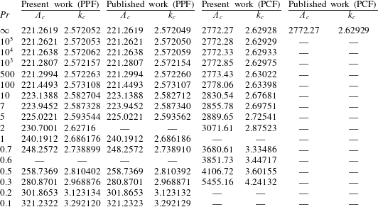
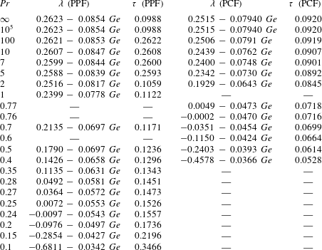
The eigenvalues of the problem, equations (3.15) and (3.16), with boundary conditions (3.17) are determined numerically with a shooting method. The accuracy and validity of the numerical scheme are checked by comparing our results with the published results of linear stability for PPF (Barletta et al. Reference Barletta, Celli and Nield2011) at varying Prandtl numbers and PCF in the limit of infinite  $Pr$ considered in Barletta & Nield (Reference Barletta and Nield2010). Table 1 presents the critical values
 $\unicode[STIX]{x1D6EC}_{c}$ and the corresponding critical wavenumbers
 $k_{c}$ for a wide range of Prandtl numbers. As can be seen from the table 1, our results are in very good agreement with the numerical computations given by Barletta et al. (Reference Barletta, Celli and Nield2011) and by Barletta & Nield (Reference Barletta and Nield2010). In particular, the critical values
 $\unicode[STIX]{x1D6EC}_{c}$ are found to match up to at least five significant digits those of Barletta et al. (Reference Barletta, Celli and Nield2011) and Barletta & Nield (Reference Barletta and Nield2010). The critical value
 $\unicode[STIX]{x1D6EC}_{c}$ at the onset of convection decreases with increasing
 $Pr$ for both PPF and PCF. The Prandtl number has therefore a destabilizing effect. We also note that the critical value
 $\unicode[STIX]{x1D6EC}_{c}$ for a fixed value of
 $Pr$ is more than ten times higher in PCF than in PPF.
Critical parameters  $\unicode[STIX]{x1D6EC}_{c}$ and
 $k_{c}$ at the onset of longitudinal rolls for different
 $Pr$ for PPF and PCF and comparison with the results of Barletta et al. (Reference Barletta, Celli and Nield2011) and by Barletta & Nield (Reference Barletta and Nield2010).

We compute the eigenfunctions with a definite normalization of the vertical component of the velocity. The normalization is chosen in a manner such that  $\int _{0}^{1}|w_{1}|^{2}\,\text{d}z=k_{c}^{2}\int _{0}^{1}|\unicode[STIX]{x1D6F9}_{1}|^{2}\,\text{d}z=1$. For the sake of conciseness, the eigenfunctions in PCF are not displayed, as they present essentially the same qualitative behaviour.
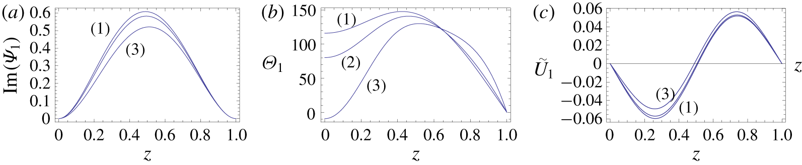
The dependence of the eigenfunctions on the vertical coordinate in PPF is shown in figure 1 for different  $Pr$. Computations indicate that the eigenfunctions
 $\unicode[STIX]{x1D6E9}_{1}$ and
 $\tilde{U} _{1}$ are real valued while
 $\unicode[STIX]{x1D6F9}_{1}$ is a pure imaginary valued. As it is shown in figure 1,
 $\text{Im}(\unicode[STIX]{x1D6F9}_{1})$ and
 $\tilde{U} _{1}$ are respectively nearly even and odd with respect to the midplane reflection symmetry, while the eigenfunction
 $\unicode[STIX]{x1D6E9}_{1}$ has asymmetric profile as a consequence of the asymmetric prescribed thermal boundary conditions. We also note that, in contrast to
 $\unicode[STIX]{x1D6F9}_{1}$ and
 $\tilde{U} _{1}$, the influence of
 $Pr$ on the vertical distribution of
 $\unicode[STIX]{x1D6E9}_{1}$ is significant. For instance, we observe that the value of
 $\unicode[STIX]{x1D6E9}_{1}$ at the lower boundary decreases with the decrease of
 $Pr$, and eventually changes sign for small Prandtl number. There is also a significant change in the vertical temperature gradient in the lower half-plane when Prandtl number varies, in comparison with the nearly constant temperature gradient in the upper plane. Note that the influence of
 $Pr$ is due to the presence of the forcing term
 $-2(\unicode[STIX]{x1D6EC}/Pr)\,f^{\prime }(z)(\unicode[STIX]{x2202}\tilde{u} _{1}/\unicode[STIX]{x2202}z)$ in the linear energy equation.
Eigenfunctions at critical conditions in PPF with different values of Prandtl number: (1)  $Pr=10^{5}$; (2)
 $Pr=1$ and (3)
 $Pr=0.27$.

3.2.2 Solutions to the second-order problem
At  $O(\unicode[STIX]{x1D700}^{2})$, the non-homogenous problem for
 $\tilde{V}_{2}$ is given at criticality by
 $$\begin{eqnarray}\displaystyle {\mathcal{L}}_{c}\,\tilde{V}_{2}=N_{2}(\tilde{V}_{1}). & & \displaystyle\end{eqnarray}$$
The term  $N_{2}$ on the right-hand side of (3.18) is the nonlinear expression
 $N$ evaluated to
 $O(\unicode[STIX]{x1D700}^{2})$. It contains known linear fundamental modes determined at
 $O(\unicode[STIX]{x1D700})$
 $(\unicode[STIX]{x1D713}_{1},\unicode[STIX]{x1D703}_{1},\tilde{u} _{1})$ and their derivatives. The nonlinear interactions between these fundamental modes and their complex conjugates generate higher harmonics and a modification of the basic state. The solutions to (3.18) are then sought in the form
 $$\begin{eqnarray}\displaystyle (\unicode[STIX]{x1D713}_{2},\unicode[STIX]{x1D703}_{2},\tilde{u} _{2}) & = & \displaystyle [A(t_{2})^{2}(\unicode[STIX]{x1D6F9}_{22}(z),\unicode[STIX]{x1D6E9}_{22}(z),\tilde{U} _{22}(z))\text{e}^{\text{i}2k_{c}y}+\text{c.c.}]\nonumber\\ \displaystyle & & \displaystyle +\,|A(t_{2})|^{2}\,(\unicode[STIX]{x1D6F9}_{20}(z),\unicode[STIX]{x1D6E9}_{20}(z),\tilde{U} _{20}(z)).\end{eqnarray}$$
Substituting expressions (3.19) into (3.18), and separating the harmonic components, one obtains a system of equations for  $(\unicode[STIX]{x1D6F9}_{22}(z),\unicode[STIX]{x1D6E9}_{22}(z),\tilde{U} _{22}(z))$ and a system of equations for
 $(\unicode[STIX]{x1D6F9}_{20}(z),\unicode[STIX]{x1D6E9}_{20}(z),\tilde{U} _{20}(z))$. The boundary conditions for
 $(\unicode[STIX]{x1D6F9}_{22}(z),\unicode[STIX]{x1D6E9}_{22}(z),\tilde{U} _{22}(z))$ and
 $(\unicode[STIX]{x1D6F9}_{20}(z),\unicode[STIX]{x1D6E9}_{20}(z),\tilde{U} _{20}(z))$ are the same as for
 $\tilde{V}_{1}$, equation (3.17).
As for the linear eigenfunctions, the nonlinear corrections are computed numerically. The properties of the nonlinear corrections at small and large Prandtl numbers are of interest. They are determined by different dominant nonlinearities defined by (3.9). For  $Pr\gg 1$, the dominant nonlinear effect lies in advection of temperature (i.e. nonlinear terms
 $N_{Adv}$) and in a part of the viscous dissipation (i.e. nonlinear terms
 $N_{Diss}^{Ge}$). While in the case of
 $Pr\ll 1$, advection of velocity prevails (i.e. nonlinear terms
 $N_{I}^{\unicode[STIX]{x1D713}}$ and
 $N_{I}^{\tilde{u} }$) together with a part of the viscous dissipation term (i.e. nonlinear terms
 $N_{Diss}^{Pr}$).
Independently of Prandtl number, numerical results indicate that
 $$\begin{eqnarray}\unicode[STIX]{x1D6F9}_{20}(z)=\tilde{U} _{20}(z)=0.\end{eqnarray}$$
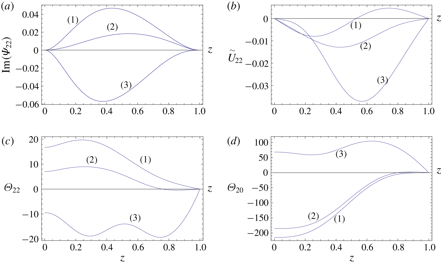
Profiles of  $\text{Im}(\unicode[STIX]{x1D6F9}_{22}(z))$,
 $\tilde{U} _{22}(z)$,
 $\unicode[STIX]{x1D6E9}_{22}(z)$ and
 $\unicode[STIX]{x1D6E9}_{20}(z)$ are shown in figure 2 for
 $Pr=10^{5}$ (curve (1)),
 $Pr=1$ (curve (2)) and
 $Pr=0.27$ (curve (3)). For
 $Pr=10^{5}$,
 $\text{Im}(\unicode[STIX]{x1D6F9}_{22}(z))$ and
 $\unicode[STIX]{x1D6E9}_{22}(z)$ are positive for all
 $z$. By considering the expressions for
 $\unicode[STIX]{x1D713}_{22}(z)$ and
 $\unicode[STIX]{x1D703}_{22}(z)$ given by (3.19), we can easily show that the effect of the first harmonics near the two vertical edges of a roll is to warm up and accelerate the upflow and to cool down and decelerate the downflow. On the other hand, for
 $Pr=0.27$,
 $\text{Im}(\unicode[STIX]{x1D6F9}_{22}(z))$ and
 $\unicode[STIX]{x1D6E9}_{22}(z)$ are negative for all
 $z$ and the effect of the first harmonic is to cool down and to decelerate the warm upflow and to warm up and accelerate the cold downflow. As a consequence we can expect that the isolines of the streamfunction stretch towards the warm upflow (the cold downflow) for
 $Pr=10^{5}$ (
 $Pr=0.27$) near the vertical edge of a roll. More importantly, the nonlinearities of the problem act to produce a temperature correction
 $\unicode[STIX]{x1D6E9}_{20}(z)$ of the basic temperature distribution that strongly depends on the Prandtl number. For
 $Pr=10^{5}$ and
 $Pr=1$, we see from figure 2(d) that this correction is negative with a positive temperature gradient except near the upper plate, while for
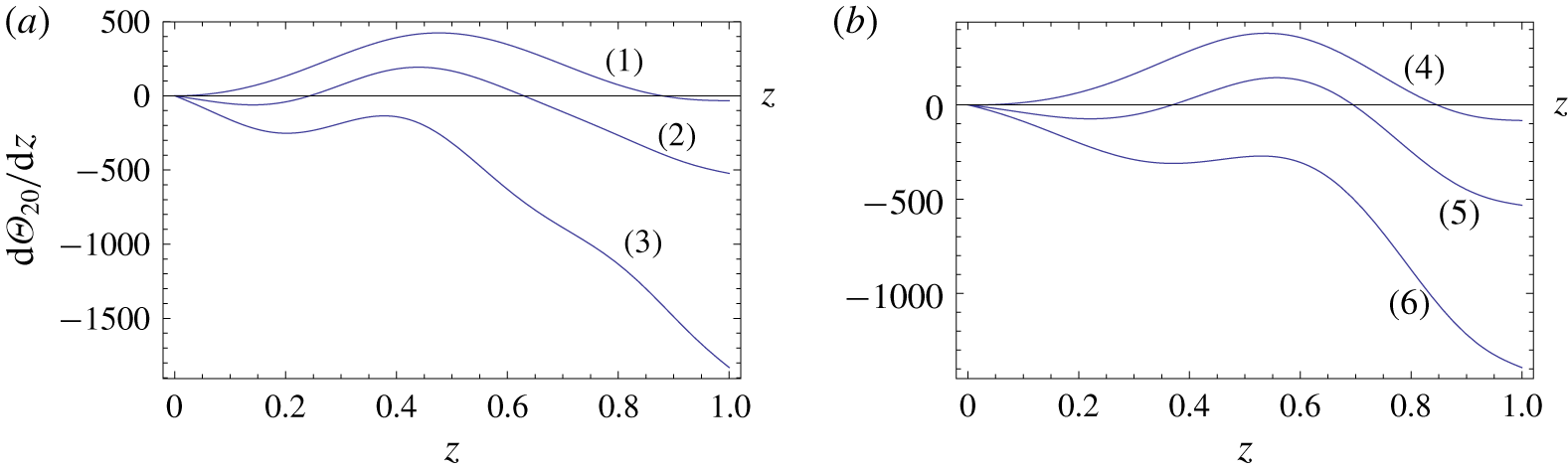
 $Pr=0.27$ the correction becomes positive with a negative temperature gradient, except for a region near the centre of the cell. A positive correction of the basic temperature gradient means that the first nonlinearities induce a stabilizing effect and one can expect a supercritical bifurcation in this case. In contrast, a negative correction of the basic temperature gradient leads to a destabilizing effect of the nonlinearities and therefore may be considered as a precursor to the emergence of a subcritical bifurcation. This is the reason why we plot, in figure 3, the vertical dependence of the nonlinear correction
 $\text{d}\unicode[STIX]{x1D6E9}_{20}/\text{d}z$ to the basic temperature gradient for
 $Pr=1$,
 $Pr=0.27$ and
 $Pr=0.15$ for PPF and
 $Pr=2$,
 $Pr=0.8$ and
 $Pr=0.5$ for PCF. This figure shows clearly that the spatial region with a positive gradient of the correction to the basic temperature shrinks as the Prandtl number decreases and eventually disappears for small
 $Pr$. As we will see later, the sign change of the nonlinear correction
 $\text{d}\unicode[STIX]{x1D6E9}_{20}/\text{d}z$ from positive to negative at small
 $Pr$ announces the transition from supercritical to subcritical bifurcation.
Vertical variations of the first nonlinear corrections to the linear mode at critical conditions in PPF with different values of Prandtl number: (1)  $Pr=10^{5}$; (2)
 $Pr=1$ and (3)
 $Pr=0.27$.

Correction of the basic temperature gradient  $\text{d}\unicode[STIX]{x1D6E9}_{20}/\text{d}z$ as a function of
 $z$: (a) PPF configuration (1)
 $Pr=1$; (2)
 $Pr=0.27$; (3)
 $Pr=0.15$ and (b) PCF configuration (4)
 $Pr=2$; (5)
 $Pr=0.8$; (6)
 $Pr=0.5$.

3.2.3 Third-order solvability condition
At  $O(\unicode[STIX]{x1D700}^{3})$, the following non-homogenous problem for
 $\tilde{V}_{3}$ is obtained:
 $$\begin{eqnarray}\displaystyle {\mathcal{L}}_{c}\,\tilde{V}_{3}=-({\mathcal{L}}^{\prime }\,\unicode[STIX]{x2202}_{t_{2}}+\unicode[STIX]{x1D6EC}_{2}\,\,{\mathcal{L}}_{2})\tilde{V}_{1}+N_{3}(\tilde{V}_{1},\tilde{V}_{2}). & & \displaystyle\end{eqnarray}$$
The nonlinear term  $N_{3}$ is the nonlinear expression
 $N$ evaluated to
 $O(\unicode[STIX]{x1D700}^{3})$.
After inserting  $\tilde{V}_{1}$ and
 $\tilde{V}_{2}$ into (3.21), there is no need to really solve this equation. Projecting instead the whole equation onto
 $\tilde{V}^{\dagger }$, where
 $\tilde{V}^{\dagger }$ is the solution to the adjoint of the linear problem, yields a solvability condition, known as the Fredholm alternative. We apply the solvability condition at
 $O(\unicode[STIX]{x1D700}^{3})$,
 $$\begin{eqnarray}\displaystyle \langle -({\mathcal{L}}^{\prime }\,\unicode[STIX]{x2202}_{t_{2}}+\unicode[STIX]{x1D6EC}_{2}\,{\mathcal{L}}_{2})\tilde{V}_{1}+N_{3},\tilde{V}^{\dagger }\rangle =0, & & \displaystyle\end{eqnarray}$$
with the appropriate scalar product,
 $$\begin{eqnarray}\displaystyle \langle \tilde{V}_{i},\tilde{V}_{j}\rangle =\frac{1}{2\unicode[STIX]{x03C0}/k_{c}}\int _{0}^{2\unicode[STIX]{x03C0}/k_{c}}\int _{0}^{1}\tilde{V}_{i}\cdot \tilde{V}_{j}^{\ast }\,\text{d}z\,\text{d}y, & & \displaystyle\end{eqnarray}$$
where  $\tilde{V}_{j}^{\ast }$ is the complex conjugate of
 $\tilde{V}_{j}$.
Re-introducing the original variables  $t=t_{2}/\unicode[STIX]{x1D700}^{2}$,
 $\unicode[STIX]{x1D6EC}_{2}=(\unicode[STIX]{x1D6EC}-\unicode[STIX]{x1D6EC}_{c})/\unicode[STIX]{x1D700}^{2}$ and
 $A=\unicode[STIX]{x1D700}\,A$ yields the cubic Landau equation for the disturbance amplitude
 $A(t)$,
 $$\begin{eqnarray}\displaystyle \unicode[STIX]{x1D70F}\,\frac{\text{d}A}{\text{d}t}=\frac{\unicode[STIX]{x1D6EC}-\unicode[STIX]{x1D6EC}_{c}}{\unicode[STIX]{x1D6EC}_{c}}\,A-\unicode[STIX]{x1D706}\,A|A|^{2}, & & \displaystyle\end{eqnarray}$$
where
 $$\begin{eqnarray}\displaystyle \unicode[STIX]{x1D70F}=\frac{1}{\unicode[STIX]{x1D6EC}_{c}}\,\frac{\langle {\mathcal{L}}^{\prime }\,\unicode[STIX]{x2202}_{t}\tilde{V}_{1},\tilde{V}^{\dagger }\rangle }{\langle \,{\mathcal{L}}_{2}\tilde{V}_{1},\tilde{V}^{\dagger }\rangle } & & \displaystyle\end{eqnarray}$$
and
 $$\begin{eqnarray}\displaystyle \unicode[STIX]{x1D706}=-\frac{1}{\unicode[STIX]{x1D6EC}_{c}}\,\frac{\langle N_{3},\tilde{V}^{\dagger }\rangle }{\langle \,{\mathcal{L}}_{2}\tilde{V}_{1},\tilde{V}^{\dagger }\rangle }. & & \displaystyle\end{eqnarray}$$
4 Results of the weakly nonlinear stability
4.1 Supercritical/subcritical bifurcation
Computations of the characteristic time of instability  $\unicode[STIX]{x1D70F}$ and the first Landau constant
 $\unicode[STIX]{x1D706}$ indicate that they are real valued. It is worth mentioning that the coefficient
 $\unicode[STIX]{x1D70F}$ depends only on
 $Pr$ whereas
 $\unicode[STIX]{x1D706}$ depends on
 $Pr$ and
 $Ge$. In table 2 we give, for both PPF and PCF configurations, the numerical values of the characteristic time of instability
 $\unicode[STIX]{x1D70F}$ as a function of
 $Pr$ and the nonlinear coefficient
 $\unicode[STIX]{x1D706}$ as a function of Gebhart number for a very wide range of
 $Pr$. The coefficient
 $\unicode[STIX]{x1D70F}$ is always positive independently of
 $Pr$ while the nonlinear coefficient
 $\unicode[STIX]{x1D706}$ is positive or negative depending on the
 $Ge$ and
 $Pr$ numbers. The sign of
 $\unicode[STIX]{x1D706}$ determines whether or not we are dealing with a subcritical bifurcation. The values of
 $\unicode[STIX]{x1D706}$ reported in table 2 indicate that independently of Gebhart number the bifurcation is subcritical (i.e.
 $\unicode[STIX]{x1D706}<0$) if
 $Pr<0.25$ for PPF and if
 $Pr<0.77$ for PCF. Otherwise, for higher Prandtl number, there exists a particular value of Gebhart number,
 $Ge^{\ast }$ such that the bifurcation is supercritical if
 $Ge<Ge^{\ast }$ or subcritical if
 $Ge>Ge^{\ast }$.
Coefficients  $\unicode[STIX]{x1D706}$ and
 $\unicode[STIX]{x1D70F}$ in Landau cubic equation for different
 $Pr$ in PPF and PCF configurations.

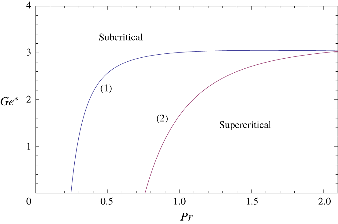
Figure 4 shows the variation of  $Ge^{\ast }$ as a function of
 $Pr$ for PPF (line 1) and for PCF (line 2). As can be seen from this figure, variations of
 $Ge^{\ast }$ become important only for
 $Pr<1$, while for usual fluids with
 $Pr>1$,
 $Ge^{\ast }$ may be approximated by its asymptotic value
 $Ge^{\ast }=3.072$ for PPF and
 $Ge^{\ast }=3.167$ for PCF, obtained in the limit of infinite Prandtl number. As the Gebhart number plays a key role in determining the supercritical or subcritical nature of the bifurcation, it is necessary to consider its realistic numerical values. From the physical point of view, high values of
 $Ge$ can occur only in geophysical or in atmospheric flows, so one can expect the occurrence of subcritical bifurcation for such flows for both small and large Prandtl numbers. In contrast to these flows, and as pointed out in Barletta et al. (Reference Barletta, Celli and Nield2011), if the fluid flow is on a typical laboratory scale, then
 $Ge$ can hardly be greater than 10-5. In this case a subcritical bifurcation is therefore restricted only to fluids with small Prandtl numbers.
Critical values  $Ge^{\ast }$ of the Gebhart number above which the bifurcation becomes subcritical versus Prandtl number.

To shed more light on the mechanism of supercritical/subcritical instability, an investigation of the effect on the first Landau constant of each of the three different nonlinear contributions present in the current problem is made. The nonlinear terms defined by (3.9) are  $N_{I}=(N_{I}^{\unicode[STIX]{x1D713}},0,N_{I}^{\tilde{u} })^{\text{T}}$,
 $N_{A}=(0,N_{Adv},0)^{\text{T}}$ and
 $N_{D}=(0,N_{Diss}^{Ge}+N_{Diss}^{Pr},0)^{\text{T}}$ and represent respectively, nonlinear inertial terms, nonlinear thermal advection terms and terms modelling the nonlinear contribution of viscous dissipation.
The Landau constant may be written as the sum of three constants
 $$\begin{eqnarray}\displaystyle \unicode[STIX]{x1D706}=\unicode[STIX]{x1D706}_{I}+\unicode[STIX]{x1D706}_{A}+\unicode[STIX]{x1D706}_{D}, & & \displaystyle\end{eqnarray}$$
where
 $$\begin{eqnarray}\displaystyle (\unicode[STIX]{x1D706}_{I},\unicode[STIX]{x1D706}_{A},\unicode[STIX]{x1D706}_{D})=-\frac{1}{\unicode[STIX]{x1D6EC}_{c}\langle \,{\mathcal{L}}_{2}\tilde{V}_{1},\tilde{V}^{\dagger }\rangle }\,(\langle N_{I},\tilde{V}^{\dagger }\rangle ,\langle N_{A},\tilde{V}^{\dagger }\rangle ,\langle N_{D},\tilde{V}^{\dagger }\rangle ). & & \displaystyle\end{eqnarray}$$
The different contributions  $\unicode[STIX]{x1D706}_{I}$,
 $\unicode[STIX]{x1D706}_{A}$ and
 $\unicode[STIX]{x1D706}_{D}$ to the Landau constant
 $\unicode[STIX]{x1D706}$ are determined by the computation of the integrals (4.2) at critical conditions (
 $\unicode[STIX]{x1D6EC}_{c}$,
 $k_{c}$) for different values of
 $Ge$ and
 $Pr$.
We found that  $\unicode[STIX]{x1D706}_{I}$ is zero independently of
 $Ge$ and
 $Pr$, meaning that the inertial terms have no influence on the nonlinear evolution of the disturbance amplitude
 $A(t)$. On the other hand, we found that
 $\unicode[STIX]{x1D706}_{A}$ is the sum of two coefficients:
 $$\begin{eqnarray}\displaystyle \unicode[STIX]{x1D706}_{A}=\unicode[STIX]{x1D706}_{Adv}+\unicode[STIX]{x1D706}_{A}^{D}. & & \displaystyle\end{eqnarray}$$
The coefficient  $\unicode[STIX]{x1D706}_{Adv}$ is due to the thermal advection term if the nonlinear viscous dissipative term is ignored (i.e.
 $\unicode[STIX]{x1D706}_{Adv}=\unicode[STIX]{x1D706}_{A}(N_{D}=0)$), while the thermal advection coefficient
 $\unicode[STIX]{x1D706}_{A}^{D}$ is strictly due to the presence of the nonlinear viscous dissipative term
 $N_{D}$. As a consequence, it is natural to define a new parameter
 $\unicode[STIX]{x1D706}_{vd}$ which measures the total contribution of the nonlinear viscous dissipative term:
 $$\begin{eqnarray}\displaystyle \unicode[STIX]{x1D706}_{vd}=\unicode[STIX]{x1D706}_{A}^{D}+\unicode[STIX]{x1D706}_{D}. & & \displaystyle\end{eqnarray}$$
Equation (4.1) is then written as
 $$\begin{eqnarray}\displaystyle \unicode[STIX]{x1D706}=\unicode[STIX]{x1D706}_{Adv}+\unicode[STIX]{x1D706}_{vd}. & & \displaystyle\end{eqnarray}$$
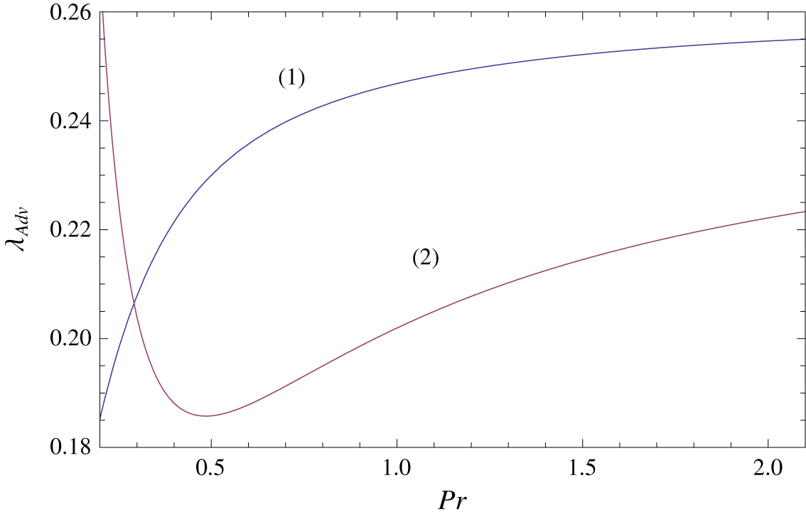
In figure 5,  $\unicode[STIX]{x1D706}_{Adv}$ is plotted as a function of
 $Pr$ for PPF (curve (1)) and for PCF (curve (2)). For both configurations,
 $\unicode[STIX]{x1D706}_{Adv}$ is positive, meaning that the effect of the nonlinear thermal advection terms is to promote supercritical bifurcation.
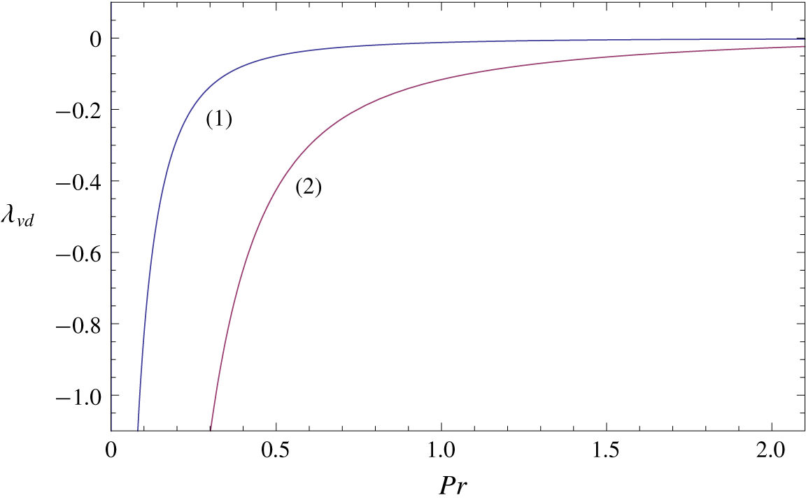
In figure 6 the dependencies of  $\unicode[STIX]{x1D706}_{vd}$ on
 $Pr$ for
 $Ge=10^{-4}$ are plotted for PPF (curve (1)) and PCF (curve (2)). As can be observed,
 $\unicode[STIX]{x1D706}_{vd}$ is negative for both configurations regardless of Prandtl number. Therefore we conclude that the nonlinear terms
 $N_{D}$ associated with the viscous dissipation promote a subcritical bifurcation. Computations of
 $\unicode[STIX]{x1D706}_{vd}$ with different Gebhart numbers lead qualitatively to the same result.
Coefficient  $\unicode[STIX]{x1D706}_{Adv}$ versus Prandtl number.

Coefficient  $\unicode[STIX]{x1D706}_{vd}$ versus Prandtl number for
 $Ge=10^{-4}$.

4.2 Stationary amplitudes in the range of validity of the weakly nonlinear analysis
The range of validity of the weakly nonlinear analysis based on the cubic amplitude equation (3.24) has to be discussed. The rigorous derivation of such an equation requires the theoretical assumption that the bifurcation parameter  $\unicode[STIX]{x1D6EC}$ is near its critical value
 $\unicode[STIX]{x1D6EC}_{c}$ at the onset of convection (i.e.
 $\unicode[STIX]{x1D716}\ll 1$). In practical applications of the weakly nonlinear analysis, the range of validity of the amplitude equations depends on the physical system under consideration. In a recent paper dealing with finite-amplitude convection and heat transfer in an inclined porous layer, Ouarzazi et al. (Reference Ouarzazi, Hirata, Barletta and Celli2017) derived a Landau equation by using a weakly nonlinear analysis. Comparing the theoretical predictions of Nusselt number with data from experiments, they found unexpectedly a very large range of validity of the derived amplitude equation, i.e.
 $\unicode[STIX]{x1D716}^{2}=2$ where
 $\unicode[STIX]{x1D716}$ measures the distance to the critical Darcy–Rayleigh number. On the other hand, Generalis & Fujimura (Reference Generalis and Fujimura2009) examined the range of validity of amplitude equations in the context of the Rayleigh–Bénard problem. They carried out a fully numerical analysis on bifurcation of steady solutions for various Prandtl numbers. Comparing two results, they showed that the amplitude equation has a wide range of validity for Prandtl number larger than
 $O(1)$. For fluids with small Prandtl numbers, on the other hand, they showed a very narrow range of validity.
In order to assess the validity of the current weakly nonlinear analysis, we use the argument made by Métivier, Nouar & Brancher (Reference Métivier, Nouar and Brancher2010) in their investigation of thermoconvective instability involving viscoplastic fluids. This argument states that the necessary condition allowing the validity of the asymptotic expansion (3.13) may be written with our notation as
 $$\begin{eqnarray}\displaystyle |A|\ll |A_{Max}|=\frac{\text{Max}(|\tilde{V}_{1}|)}{\text{Max}(|\tilde{V}_{2}|)}. & & \displaystyle\end{eqnarray}$$
We observe from numerical results shown in figures 1 and 2 for PPF that  $\text{Max}(|\tilde{V}_{1}|)=\text{Max}(|\unicode[STIX]{x1D6E9}_{1}(z)|)$ and
 $\text{Max}(|\tilde{V}_{2}|)=\text{Max}(|\unicode[STIX]{x1D6E9}_{20}(z)|)$ for the three fixed values of Prandtl number. The condition (4.6) implies
 $|A_{Max}|=0.69$; 0.76; 1.86 respectively for
 $Pr=10^{5};Pr=1;Pr=0.27$. In the same manner, for PCF we found that
 $|A_{Max}|=0.68$; 0.95; 1.74 respectively for
 $Pr=10^{5};Pr=2;Pr=0.77$.
The amplitude equation (3.24) predicts supercritical instability if the Landau constant  $\unicode[STIX]{x1D706}$ is positive, with a stable stationary nonlinear equilibrium solution:
 $$\begin{eqnarray}\displaystyle |A_{s}|=\left|\frac{\unicode[STIX]{x1D6EC}-\unicode[STIX]{x1D6EC}_{c}}{\unicode[STIX]{x1D706}\unicode[STIX]{x1D6EC}_{c}}\right|^{1/2}. & & \displaystyle\end{eqnarray}$$
If  $\unicode[STIX]{x1D706}$ is negative, a subcritical instability is predicted with the threshold amplitudes
 $|A_{s}|$, which limits the basin of attraction of the linearly stable PPF and PCF flows for
 $\unicode[STIX]{x1D6EC}<\unicode[STIX]{x1D6EC}_{c}$. In that case, the cubic amplitude equation (3.24) does not provide any stable finite-amplitude equilibrium and therefore it is necessary to carry the analysis to higher orders in amplitude. This task is out of the scope of the present work.
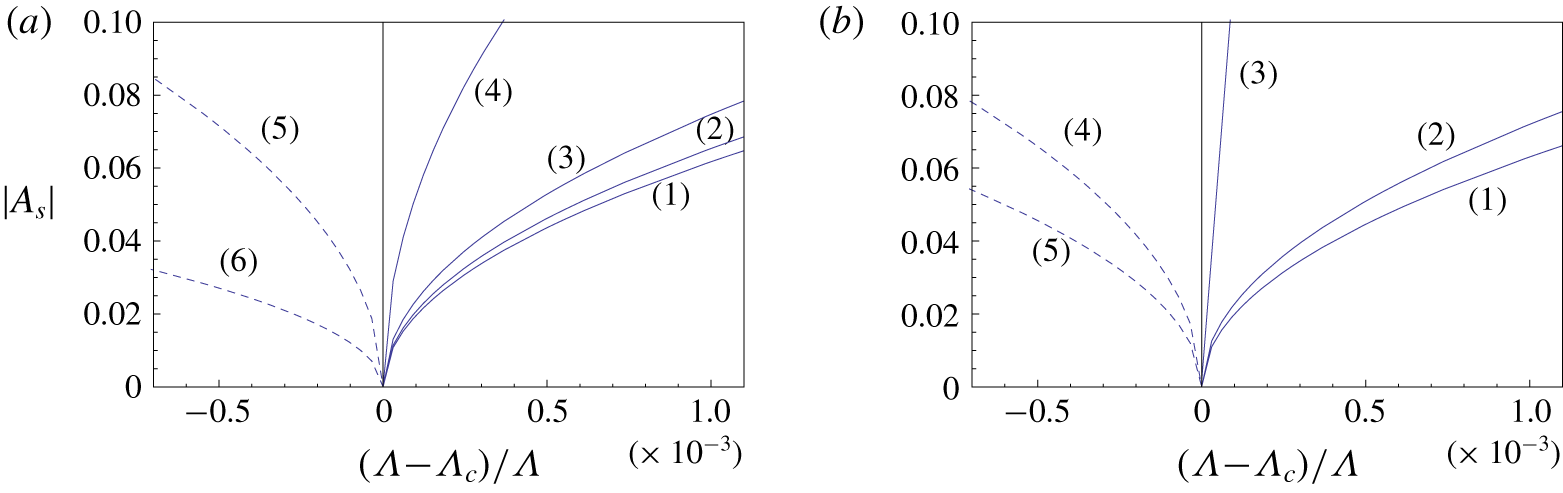
Figure 7 presents the bifurcation diagrams for different Prandtl numbers showing the equilibrium amplitudes (up to  $|A_{s}|=0.1\ll |A_{Max}|$) when the bifurcations are supercritical (continuous lines) and the threshold amplitudes (dashed lines) when the bifurcations are subcritical. The magnitude of
 $|A_{s}|$ for fixed values of
 $((\unicode[STIX]{x1D6EC}-\unicode[STIX]{x1D6EC}_{c})/\unicode[STIX]{x1D6EC}_{c})$ decreases on increasing the value of
 $Pr$ in the case of supercritical bifurcations. While for subcritical bifurcations, the bifurcation diagrams indicate that the threshold amplitude decreases with the decrease of
 $Pr$, meaning that the basic PPF and PCF flows become strongly sensitive to finite amplitude perturbations when
 $Pr$ is decreased.
Stationary amplitude as a function of the distance to criticality for  $Ge=10^{-4}$: (a) PPF configuration (1)
 $Pr=10^{5}$; (2)
 $Pr=1$; (3)
 $Pr=0.5$; (4)
 $Pr=0.27$; (5)
 $Pr=0.2$; (6)
 $Pr=0.1$ and (b) PCF configuration (1)
 $Pr=10^{5}$, (2)
 $Pr=2$, (3)
 $Pr=0.77$; (4)
 $Pr=0.6$; (5)
 $Pr=0.5$.

4.3 Heat transfer
The conductive state supports a non-uniform heat flux  $J_{cond}(z)=-(\text{d}T_{b}/\text{d}z)$ flowing vertically through the layer. The expression for the basic temperature
 $T_{b}(z)$ is given by (2.8). In the presence of a convective velocity field, the total stationary vertical flux is
 $J=J_{cond}(z)+J_{conv}(y,z)$, where
 $J_{conv}$ is independent of
 $x$ for longitudinal rolls with the axis along the
 $x$ direction and it reads
 $$\begin{eqnarray}\displaystyle J_{conv}(y,z)=-\frac{\unicode[STIX]{x2202}\unicode[STIX]{x1D713}}{\unicode[STIX]{x2202}y}(T_{b}+\unicode[STIX]{x1D703})-\frac{\text{d}\unicode[STIX]{x1D703}}{\text{d}z}. & & \displaystyle\end{eqnarray}$$
The contribution  $-(\unicode[STIX]{x2202}\unicode[STIX]{x1D713}/\unicode[STIX]{x2202}y)(T_{b}+\unicode[STIX]{x1D703})$ to the convective flux
 $J_{conv}$ describes convective transport of heat by the velocity field. The term
 $-(\text{d}\unicode[STIX]{x1D703}/\text{d}z)$ is the diffusive flux of heat, driven by the gradient in the convection-generated deviations of the temperature field from the conduction profile.
We define the lateral average convective heat flux by
 $$\begin{eqnarray}\displaystyle \langle J_{conv}\rangle (z)=\frac{1}{2\unicode[STIX]{x03C0}/k_{c}}\int _{0}^{2\unicode[STIX]{x03C0}/k_{c}}J_{conv}(y,z)\,\text{d}y. & & \displaystyle\end{eqnarray}$$
We remark that, owing to the boundary conditions (3.10) imposed at  $z=0$ and
 $z=1$,
 $J_{conv}(z=0)=0$ and
 $J_{conv}(z=1)=-(\text{d}\unicode[STIX]{x1D703}/\text{d}z)(z=1)$. This means that the average heat flux
 $\langle J_{conv}\rangle (z)$ is
 $z$ dependent and it is therefore instructive to investigate its vertical distribution in the fluid layer.
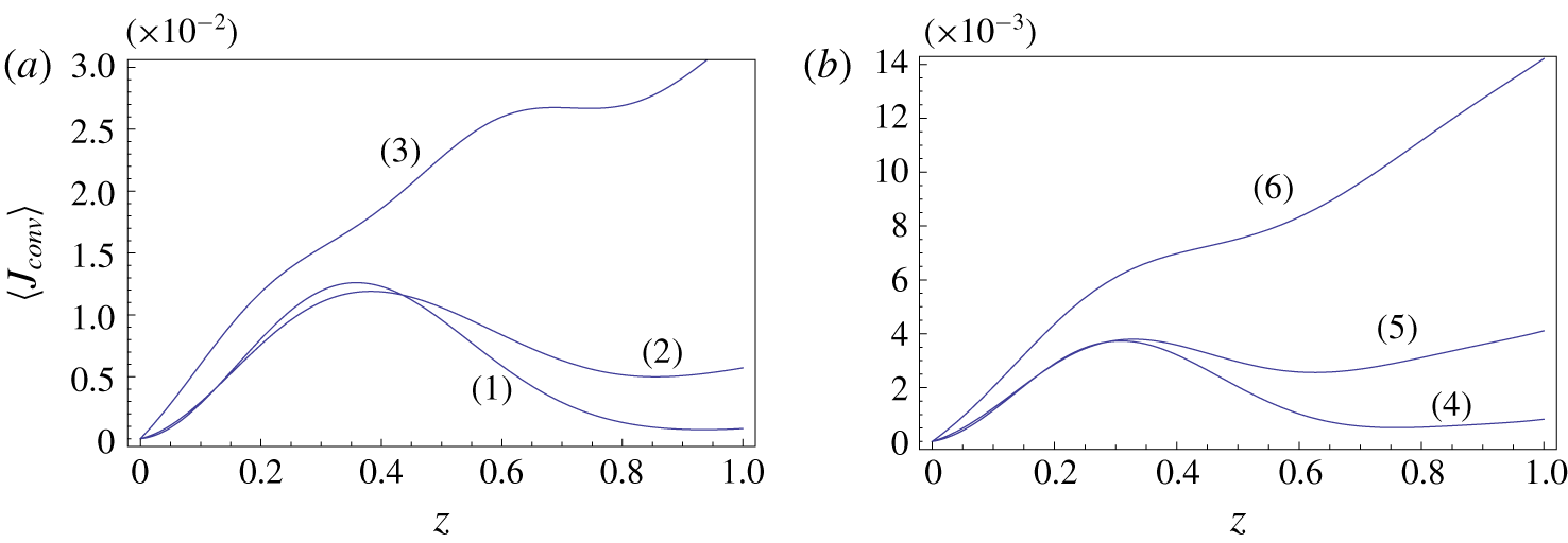
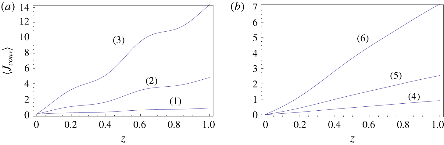
Figures 8 and 9 show typical plots of the vertical variations of the average heat flux  $\langle J_{conv}\rangle (z)$ for (a) PPF and (b) PCF at
 $\unicode[STIX]{x1D6EC}=1.1\unicode[STIX]{x1D6EC}_{c}$,
 $Ge=10^{-4}$ and various Prandtl numbers corresponding to supercritical bifurcations. Figure 8 shows results for some high or moderate Prandtl numbers while figure 9 focuses on the regime of small Prandtl numbers. The average heat flux is found to be some orders of magnitude smaller at high Prandtl numbers than at small ones. On the other hand, the average heat flux exhibits a maximum located near the middle of the fluid layer at high Prandtl numbers. As the Prandtl number decreases, this maximum moves to the top and eventually reaches the upper boundary.
Vertical distribution of average convective heat flux at  $(\unicode[STIX]{x1D6EC}-\unicode[STIX]{x1D6EC}_{c}/\unicode[STIX]{x1D6EC}_{c})=10^{-3}$ for fluids with moderate and high Prandtl numbers: (a) PPF configuration (1)
 $Pr=10^{5}$; (2)
 $Pr=5$ and (3)
 $Pr=2$ and (b) for PCF configuration (4)
 $Pr=10^{5}$, (5)
 $Pr=20$, (6)
 $Pr=10$.

Vertical distribution of average convective heat flux at  $(\unicode[STIX]{x1D6EC}-\unicode[STIX]{x1D6EC}_{c}/\unicode[STIX]{x1D6EC}_{c})=10^{-3}$ for fluids with small Prandtl number: (a) PPF configuration (1)
 $Pr=0.5$, (2)
 $Pr=0.31$, (3)
 $Pr=0.27$ and (b) PCF configuration (4)
 $Pr=1.5$, (5)
 $Pr=1.1$, (6)
 $Pr=0.9$.

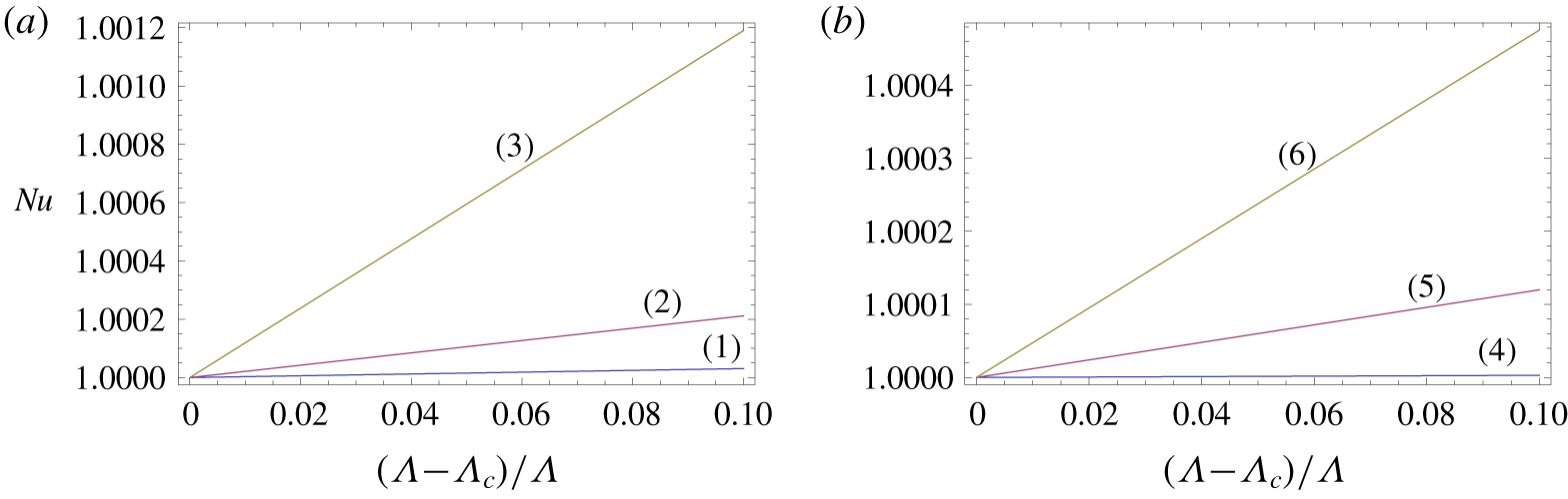
Our aim now is to find the relation between the total heat flux and the heat flux in the conductive regime, transferred to the upper boundary. The relative contributions of conduction and convection to heat transferred to the upper plate is expressed using dimensionless Nusselt number  $Nu$ defined by
 $$\begin{eqnarray}\displaystyle Nu(z=1)=1+\frac{\langle J_{conv}(z=1)\rangle }{J_{cond}(z=1)}, & & \displaystyle\end{eqnarray}$$
which may be written as
 $$\begin{eqnarray}\displaystyle & \displaystyle Nu=1-\frac{1}{12\unicode[STIX]{x1D6EC}}|A_{s}|^{2}\left.\frac{\text{d}\unicode[STIX]{x1D6E9}_{20}}{\text{d}z}\right|_{z=1}\quad \text{for PPF}, & \displaystyle\end{eqnarray}$$
 $$\begin{eqnarray}\displaystyle & \displaystyle Nu=1-\frac{1}{\unicode[STIX]{x1D6EC}}|A_{s}|^{2}\left.\frac{\text{d}\unicode[STIX]{x1D6E9}_{20}}{\text{d}z}\right|_{z=1}\quad \text{for PCF}. & \displaystyle\end{eqnarray}$$
According to figure 3, we notice that  $(\text{d}\unicode[STIX]{x1D6E9}_{20}/\text{d}z)|_{z=1}$ is negative and its absolute value decreases with increasing Prandtl number. The same trend is observed in the plots of
 $|A_{s}|$ shown in figure 7. Consequently, the Nusselt number evaluated at the upper plate decreases with increasing Prandtl number. Substituting the solution of
 $|A_{s}|$ given by (4.7) into (4.11) and (4.12) yields the following relationships:
 $$\begin{eqnarray}\displaystyle & \displaystyle Nu=1-\frac{1}{12\unicode[STIX]{x1D706}\unicode[STIX]{x1D6EC}_{c}}\,\left.\frac{\text{d}\unicode[STIX]{x1D6E9}_{20}}{\text{d}z}\right|_{z=1}\left(\frac{\unicode[STIX]{x1D6EC}-\unicode[STIX]{x1D6EC}_{c}}{\unicode[STIX]{x1D6EC}}\right)\quad \text{for PPF}, & \displaystyle\end{eqnarray}$$
 $$\begin{eqnarray}\displaystyle & \displaystyle Nu=1-\frac{1}{\unicode[STIX]{x1D706}\unicode[STIX]{x1D6EC}_{c}}\,\left.\frac{\text{d}\unicode[STIX]{x1D6E9}_{20}}{\text{d}z}\right|_{z=1}\left(\frac{\unicode[STIX]{x1D6EC}-\unicode[STIX]{x1D6EC}_{c}}{\unicode[STIX]{x1D6EC}}\right)\quad \text{for PCF}. & \displaystyle\end{eqnarray}$$
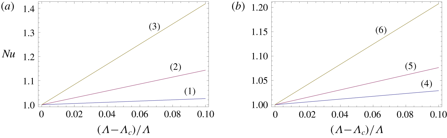
The variation of Nusselt number at the upper plate for PPF and PCF as a function of  $((\unicode[STIX]{x1D6EC}-\unicode[STIX]{x1D6EC}_{c})/\unicode[STIX]{x1D6EC})$ is shown in figure 10 for some small Prandtl numbers and in figure 11 for moderate to high values of Prandtl number. Comparing the two figures we remark, as expected, that the slopes of Nusselt number
 $S=-(1/12\unicode[STIX]{x1D706}\unicode[STIX]{x1D6EC}_{c})\,(\text{d}\unicode[STIX]{x1D6E9}_{20}/\text{d}z)|_{z=1}$ for PPF and
 $S=-(1/\unicode[STIX]{x1D706}\unicode[STIX]{x1D6EC}_{c})\,(\text{d}\unicode[STIX]{x1D6E9}_{20}/\text{d}z)|_{z=1}$ for PCF decrease drastically with the increase of Prandtl number.
Nusselt number in the regime of small Prandtl numbers: (a) PPF configuration (1)  $Pr=0.5$, (2)
 $Pr=0.31$, (3)
 $Pr=0.27$ and (b) PCF configuration (4)
 $Pr=1.5$, (5)
 $Pr=1.1$, (6)
 $Pr=0.9$.

Nusselt number in the regime of moderate and high Prandtl numbers: (a) PPF configuration (1)  $Pr=10^{5}$; (2)
 $Pr=5$ and (3)
 $Pr=2$ and (b) PCF configuration (4)
 $Pr=10^{5}$, (5)
 $Pr=20$, (6)
 $Pr=10$.

5 Conclusions
A linear and weakly nonlinear stability analysis of mixed convection in a plane parallel channel has been carried out. Both the basic solutions of Couette and Poiseuille flow have been considered. The effect causing the unstable thermal stratification and, as a consequence, the emergence of convection cells is the viscous dissipation. This effect is the sole cause of the vertical temperature gradient in the basic state, as no thermal forcing is imposed through the boundary walls. In fact, the lower wall has been assumed to be thermally insulated, while the upper wall is considered as isothermal.
The linear analysis has been surveyed relying on the previous studies by Barletta & Nield (Reference Barletta and Nield2010) and Barletta et al. (Reference Barletta, Celli and Nield2011). The results presented by these authors have been recovered and extended. The important result that the critical condition for the onset of convective instability is triggered by longitudinal rolls has been highlighted as the basis for the weakly nonlinear analysis.
The study of the nonlinear behaviour has been carried out within the weakly nonlinear theory. We numerically obtained the linear fundamental modes and showed that their nonlinear interaction generates a modification of the basic temperature gradient. The effect of Prandtl number,  $Pr$, on the correction of the basic temperature gradient induced by the first nonlinearities is examined. It emerges that this correction is globally positive for high and moderate
 $Pr$, while it becomes negative for all vertical positions of the medium for small
 $Pr$. Physically, a negative modification of the basic temperature gradient discloses a destabilizing effect of the first nonlinearities and may be regarded as a signature of the presence of a subcritical bifurcation. The coefficients of the appropriate cubic Landau amplitude equation, which describes stationary convection patterns beyond the instability threshold, have been computed for longitudinal rolls. The main results obtained through this analysis are the following:
(i) There exists a threshold value,
 $Ge^{\ast }$, of the Gebhart number, $Ge$, such that a supercritical bifurcation happens when $Ge<Ge^{\ast }$, while the bifurcation is subcritical for $Ge>Ge^{\ast }$. The value of $Ge^{\ast }$ depends on $Pr$, both for the Couette and the Poiseuille flow.
(ii) The effects of the three nonlinear terms in the governing equations, inertia, advection and viscous dissipation, have been discerned. The inertia term turned out to be ineffective as its contribution to the Landau constant is zero. The advection term tends to favour a supercritical bifurcation, while the dissipation term promotes a subcritical bifurcation.
(iii) The heat transfer mechanism has been investigated in the case of a supercritical bifurcation by evaluating both the lateral average convective heat flux and the Nusselt number. The maximum average heat flux is found to be located near the middle of the fluid layer at high
$Pr$ while this maximum occurs at the upper boundary for small $Pr$. As a consequence, the Nusselt number evaluated at the upper boundary is reduced with the increase of $Pr$.


In this paper, we showed that for realistic values of the Gebhart number a high viscous dissipation effect reduces the subcritical character of the bifurcation, which may become supercritical for fluids with large  $Pr$. However, it would be desirable to go beyond the cubic Landau amplitude equation by considering higher nonlinearities in order to compute the equilibrium amplitude for fluids with small
 $Pr$ which yield a subcritical bifurcation. This task will be the objective of a future paper.
Declaration of interests
The authors report no conflict of interest.