1. Introduction
In recent years, redundant manipulators have been playing an increasingly important role in various fields, including industry [Reference Xie, Chen, Zhang, Li and Rong1], space exploration [Reference Zhang, Liu, Ning, Li, Liu and Lu2], and others [Reference Li, Feng, Zhang, Peng, Ma, Liu, Ru, Sun and Zhao3, Reference Yuan, Li and Su4]. In these scenarios, the most common task for redundant manipulators is to move the end-effector from the starting position to the target position, such as in assembly tasks and handling tasks. Researchers have divided the operation process of redundant manipulators into two research parts. The first part is path planning, which involves planning a feasible point-to-point path in the environment to enable the end-effector to reach the target point. The second part is trajectory planning, which involves converting the path points of the end-effector into joint information with a time sequence for the redundant manipulator. Moreover, due to the complex environment and the structural limitations of the manipulator itself, other subtasks need to be performed simultaneously during path and trajectory planning. For example, obstacle avoidance [Reference Yang, Li, Xu and Zhang5, Reference Khan, Li and Luo6] and joint physical limit avoidance [Reference Cong, Du, Chen, Zhu and Wen7, Reference Guo and Zhang8].
Traditional motion planning methods for redundant manipulators usually separate path planning and trajectory planning into a two-step inverse solution. The manipulator end-effector is abstracted as a point or sphere in path planning, and feasible paths present in the environment are searched using algorithms such as Rapidly-Exploring Random Tree (RRT) algorithm [Reference Feng, Jiang, Li, Zhou, Bi and Part9], A* algorithm, artificial potential field method [Reference Zhang, Wu and Shen10, Reference Gammell, Barfoot and Srinivasa11], and metaheuristic [Reference Khan and Ijaz12]. In trajectory planning, researchers usually use approaches such as the gradient projection method, the extended Jacobi method, and the optimization function solution method [Reference Ju, Jin, Wang and Zhao13–Reference Liu, Tong, Ju and Liu15]. Trajectory planning involves solving the inverse kinematics (IK) of the manipulator to obtain joint angles, angular velocities, and angular accelerations from the smoothed path points. Although the integration of the above algorithms has effectively addressed the motion planning task for manipulators, there are still some issues that cannot be ignored. First, both RRT and A* path planning algorithms require the pre-construction of an environment map, and they lack extendibility in dealing with unknown environments, and may even suffer from the curse of high dimensionality. Moreover, these path planning algorithms do not take into account the actual physical configuration of the manipulator. However, it is not only the end-effector that needs to avoid obstacles, but all the links of the manipulator must not come into contact with obstacles during motion. Second, solving the IK is difficult [Reference Ma, Xie, Zhan, Jiang, Liu and Liu16, Reference Peng, Tang, Huang and Wei17]. Since the joint dimension of redundant manipulators is greater than the dimension of the environment, the calculation of the inverse of the Jacobian matrix is very complex and there are multiple solutions. Furthermore, due to the need to consider the links of the manipulator avoiding obstacles (especially irregular obstacles) and joint position constraints, the inverse kinematic solution may face no solution or singular solutions.
In recent years, research at the intersection of deep reinforcement learning (DRL) and robotics has provided new solutions for today’s robotics [Reference Zhang, Ju and Cao18, Reference Khlif, Nahla and Safya19]. In robot path planning, DRL does not require the construction of an environment map [Reference Bai, Pang, He, Zhao and Wang20, Reference Gan, Huo and Li21]. The agent learns to obtain the optimal policy output. Moreover, when facing high-dimensional environments, since the policy is approximated using neural networks, there is no risk of dimensionality explosion. In trajectory planning, DRL has been studied mainly in place of the inverse kinematic solution process [Reference Ying, Liu, Jiang and Yin22]. The manipulator learns through continuous interaction with the environment to approximate the neural network function representing the IK, thereby avoiding the complex calculation of the Jacobian matrix and improving the efficiency of trajectory planning and the quality of the optimized solution [Reference Cao, Wang, Zheng and Liu23, Reference Song, Li, Liu and Wang24]. However, DRL also has problems such as slow training speed and non-convergence, mainly due to insufficient environment feature extraction and improper reward function settings [Reference De Witte, Van Hauwermeiren, Lefebvre and Crevecoeur25, Reference Sui, Pu, Yi and Wu26]. Moreover, the aforementioned reinforcement learning algorithms only improve the speed of motion planning and environmental adaptability, but do not change the motion planning method of first performing path planning and then trajectory planning. In recent years, Dai et al. [Reference Dai, Zhang and Deng27] designed a motion planning scheme for manipulators in the joint space, combining artificial potential fields and the RRT algorithm, to avoid complex IK calculations and improve obstacle avoidance efficiency. Liu et al. [Reference Liu, Ying, Jiang, Shan and Shen28] proposed a general framework based on DRL, where the output of the policy function is mapped to the joint space. This not only saves the process of solving IK for trajectory planning but also allows for timely replanning when the task scenario changes. Although refs. [Reference Dai, Zhang and Deng27, Reference Liu, Ying, Jiang, Shan and Shen28] use different algorithms, the basic idea is the same: to use the joint space as the output of motion planning and employ the forward kinematics model instead of the IK model. This idea is different from the traditional two-step motion planning method and provides a new direction for solving motion planning problems. However, both algorithms employ the artificial potential field method for obstacle avoidance, abstracting the target point and obstacles as points that provide attractive and repulsive forces, which may lead to some incorrect solution sets. Moreover, both algorithms use joint angles as the output. To meet the requirements of motion planning, there may be abrupt changes in joint angles. However, in practical applications, such ideal abrupt changes do not exist because they would generate significant torques, which could damage the manipulator.
To address the aforementioned issues, this paper proposes a motion planning scheme for redundant manipulators to avoid obstacles based on a DRL algorithm, considering the actual shapes of obstacles. This scheme integrates the forward kinematics model of the manipulator into the DRL framework, which can not only solve the path planning task for the end-effector but also perform obstacle avoidance trajectory planning for all joints and links of the manipulator. The specific contributions are as follows:
-
1. A DRL algorithm scheme that uses joint accelerations as policy outputs is proposed. By employing multilevel physical limit avoidance for joints, it not only prevents the generation of large torques but also meets the motion planning task without IK solving.
-
2. The Gilbert–Johnson–Keerthi (GJK) distance algorithm is integrated into the DRL scheme to obtain the accurate real-time distance between the manipulator and irregular convex polyhedral obstacles, providing support for the construction of a composite reward function.
-
3. A composite reward function mainly constructed from joint accelerations and velocities is proposed. This function aims to achieve collision-free motion for both the end-effector and the manipulator links. It takes into account the position error between the end-effector and the target point, as well as the actual minimum distance between the links and the obstacles.
The remainder of this paper is organized as follows. Section 2 presents the overall framework of the motion planning. Section 3 introduces the design details of the motion planning scheme, including the establishment of the manipulator’s kinematics model and the joint physical limit mechanism, the idea of the GJK algorithm, and the framework of the DRL algorithm. Section 4 describes the construction of the composite reward function. Section 5 provides the simulation and experimental verification and analysis. Section 6 summarizes the method and proposes future research directions.
2. Overall framework of motion planning
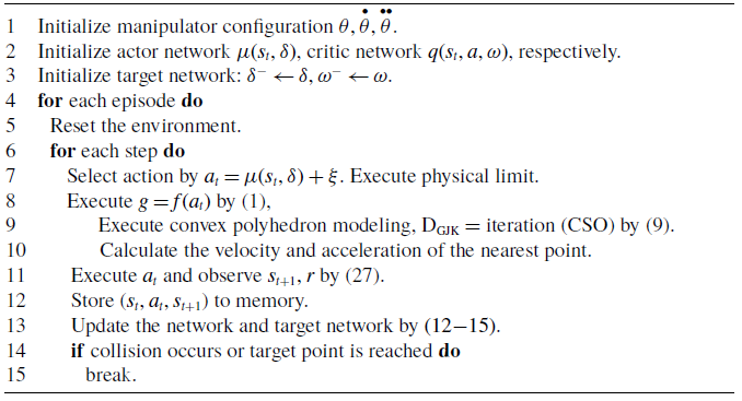
The overall motion planning scheme in this paper can be divided into three parts, including the kinematics modeling of the manipulator, the GJK distance algorithm, and the DRL algorithm. In Figure 1, first, the physical configuration is obtained from the kinematics model of the manipulator. Then, the links of the manipulator and the obstacles are abstracted as convex polyhedron, and the GJK distance algorithm is used to obtain the coordinates of the nearest point to the obstacle. Second, through the forward kinematics model and coordinate locking, the velocity and acceleration parameters of the point on the manipulator that is closest to the obstacle are obtained. These parameters are provided to the reward function in reinforcement learning, and the network parameters are updated through the learning mechanism. Finally, the updated reinforcement learning outputs the angular acceleration for the next state. After passing through the physical joint limit, the forward kinematics model is used to update the physical configuration of the manipulator. By integrating the above three steps, a closed loop of the motion planning scheme is formed. The pseudocode for the overall scheme is shown in Algorithm 1.
Overall framework of motion planning.

3. Design of the motion planning scheme
3.1. Construction of the manipulator kinematics model
The forward kinematics model of the manipulator can be expressed as
 \begin{equation} g_{E}=f\left(\theta \right) \end{equation}
where
 $g_{E}\in R^{m}$
and
 $\theta \in R^{n}$
are the Cartesian path of the end-effector and the joint angle between the links, respectively.
 $m\gt 0$
and
 $n\gt 0$
are the dimensions of the operational space and the degree of freedom (DOF) of the manipulator, respectively. When
 $n\gt m$
, the DOF of the manipulator is greater than the dimensions of the operational space, allowing it to perform additional subtasks.
Taking the time derivative of (1) yields the velocity-level forward kinematics formula:
 \begin{equation} \overset{\bullet}{g}_{E}=J_{E}\overset{\bullet }{\theta } \end{equation}
where
 $\overset{\bullet}{g_{E}}\in R^{m}$
and
 $\overset{\bullet}{\theta }\in R^{n}$
are the velocities of the end-effector and the joint angular velocities between the links, respectively.
 $J_{E}\in R^{m\times n}$
is the Jacobian matrix of the end-effector, denoted as
 $J_{E}=\partial f(\theta )/\partial (\theta )$
.
Taking the time derivative of (2) yields the acceleration-level forward kinematics formula:
 \begin{equation} \overset{\bullet \bullet }{g}_{E}=\overset{\bullet}{J}_{E}\overset{\bullet}{\theta }+J_{E}\overset{\bullet \bullet }{\theta } \end{equation}
where
 $\overset{\bullet \bullet }{g_{E}}\in R^{m}$
and
 $\overset{\bullet \bullet }{\theta }\in R^{n}$
are the accelerations of the end-effector and the joint angular accelerations between the links, respectively.
 $\overset{\bullet}{J}_{E}\in R^{m\times n}$
is the derivative of
 $J_{E}$
with respect to time
 $t$
.
In practical engineering applications, to ensure the safety and reliability of the manipulator during operation, the following physical limits for joint variables are defined:
 \begin{equation} \begin{array}{l} \theta ^{-}\leq \theta \leq \theta ^{+}\\ \overset{\bullet}{\theta }^{_{_-}}\leq \overset{\bullet}{\theta }\leq \overset{\bullet}{\theta }^{_{_+}}\\ \overset{\bullet \bullet }{\theta }^{_{_-}}\leq \overset{\bullet \bullet }{\theta }\leq \overset{\bullet \bullet }{\theta }^{_{_+}} \end{array} \end{equation}
where
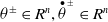 $\theta^{\pm}\in R^{n} , \overset{\bullet}{\theta}^{_{_{\pm}}}\in R^{n}$
and
 $\overset{\bullet \bullet }{\theta}^{_{_{\pm}}}\in R^{n}$
are the upper and lower limits of angle, angular velocity, and angular acceleration, respectively. The joint variables physical limits in (4) are unified as acceleration levels:
 \begin{equation} \zeta ^{-}\leq \overset{\bullet \bullet }{\theta }\leq \zeta ^{+} \end{equation}
where
 $\zeta ^{-}\in R^{n} , \zeta ^{+}\in R^{n}$
,denoted by
 \begin{align} \begin{array}{l} \zeta ^{-}=\max \big[\kappa _{p}\big(\mu \theta ^{-}-\theta \big),\kappa _{\nu }\big(\overset{\bullet}{\theta }^{_{_-}}-\overset{\bullet}{\theta }\big),\overset{\bullet \bullet }{\theta }^{_{_-}}\big]\\[10pt] \zeta ^{+}=\min \big[\kappa _{p}\big(\mu \theta ^{+}-\theta \big),\kappa _{\nu }\big(\overset{\bullet}{\theta }^{_{_+}}-\overset{\bullet}{\theta }\big),\overset{\bullet \bullet }{\theta }^{_{_+}}\big] \end{array} \end{align}
where
 $\mu \in (0,1)$
defines the critical regions
 $[\theta ^{-},\mu \theta ^{-}]$
and
 $[\mu \theta ^{+},\theta ^{+}]$
such that deceleration is performed by limiting the angular acceleration when the joint angle enters one of the critical regions. Furthermore,
 $\kappa _{p}\gt 0$
and
 $\kappa _{\nu }\gt 0$
determine the deceleration amplitude [Reference Ma, Xie, Zhan, Jiang, Liu and Liu16, Reference Zhang, Guo and Ma29].
Remark 1: Generally, the selection of a and b should ensure that the feasible region of joint acceleration c obtained from joint limits and joint velocity limits is not smaller than the feasible region obtained from the original joint acceleration.
3.2. GJK distance algorithm
Traditional distance algorithms in Cartesian coordinates do not effectively search for the shortest distance between the manipulator and obstacles in three-dimensional space, especially when the obstacles are not regular polyhedron or spheres. Therefore, researchers commonly use the artificial potential field method to establish the distance relationship between the manipulator and obstacles. However, the uniformly divergent repulsive or attractive forces generated by the artificial potential field method in space can lead to local optimal solutions in the solution space. That is, when the target point and the obstacle are very close, the manipulator may become trapped in a dilemma.
Schematic of GJK algorithm distance calculation.

The GJK algorithm iteratively abstracts objects of any shape into convex polyhedral envelopes and accurately determines the closest points between these two convex bodies, thereby yielding their actual minimum distance [Reference Gilbert, Johnson and Keerthi30, Reference Montanari, Petrinic and Barbieri31]. In Figure 2(a), there are two convex polyhedral objects
 $P$
and
 $Q$
, with their point sets in space being
 $Z_{P}\in R^{3}$
and
 $Z_{Q}\in R^{3}$
. For these two convex polyhedrons, the nearest Euclidean distance
 $d(P,Q)$
can be expressed as
 \begin{equation} d\left(P,Q\right)=\min \left\{\left\| x_{p}-x_{q}\right\| ,x_{p}\in Z_{P},x_{q}\in Z_{Q}\right\} \end{equation}
In Figure 2(b), the Minkowski difference between two objects
 $P$
and
 $Q$
in the GJK distance algorithm leads to a configuration space obstacle (CSO):
 \begin{equation} CSO=P-Q=\left\{x_{p}-x_{q},x_{p}\in Z_{P},x_{q}\in Z_{Q}\right\} \end{equation}
By using the support function to selectively calculate the above Minkowski difference, an iterative generation of a simplex polyhedron is performed. The distance between
 $P$
and
 $Q$
is equal to the nearest distance from the simplex polyhedron
 $M$
to the origin when the iteration termination condition is met. The point set of the simplex
 $M$
is
 $Z_{M}\in R^{3}$
. Hence, the existence:
 \begin{equation} d\left(P,Q\right)=\min \left\{\left\| m\right\| ,m\in Z_{M}\right\} \end{equation}
At this point, two convex polyhedron
 $P$
and
 $Q$
collide if the simplex
 $M$
contains the origin. It is worth noting that even if the objects being calculated are non-convex, the GJK distance algorithm can still identify the vertex coordinates that form the simplex during its iterative process.
3.3. DRL algorithm design
In DRL, the motion tasks of a robotic arm can be regarded as Markov decision processes (MDPs). The improvements proposed in this paper for manipulator motion planning are applicable to general reinforcement learning algorithms. However, algorithms such as Q-learning and SARSA have discrete action outputs, which may lead to the omission of correct manipulator configurations during the learning process. Although algorithms like Proximal Policy Optimization and Soft Actor-Critic can produce continuous actions, they have numerous hyperparameters that may introduce unknown effects on the proposed improvements in this paper. Therefore, this paper employs the more stable TD3 (Twin Delayed Deep Deterministic Policy Gradient) algorithm to validate the motion planning scheme for the manipulator.
For the joint exploration actions driven by DRL, each pose is the IK solution of a complex model in traditional research [Reference Sui, Pu, Yi and Wu26, Reference Wang, Frazelle, Wagner and Walker32]. Therefore, in this paper, the joint angular acceleration between each linkage is proposed as the strategy network output
 $a_{t}$
, defined as
 \begin{equation} a_{t}=\left[\overset{\bullet \bullet }{\theta }_{1},\overset{\bullet \bullet }{\theta }_{2},\cdots ,\overset{\bullet \bullet }{\theta }_{i}\right] \end{equation}
where
 $\overset{\bullet \bullet }{\theta }_{i}$
is the angular acceleration of the
 $i$
th joint. The state
 $s_{t}$
is defined as
 \begin{equation} s_{t}=\left[C_{0},C_{1},E,A_{an},A_{sp},A_{ac},D\right] \end{equation}
where
 $C_{0}=(x_{0},y_{0},z_{0})$
and
 $C_{1}=(x_{1},y_{1},z_{1})$
are the current positions of the end-effector and the target point based on the world coordinate system.
 $E=[{\unicode[Arial]{x0394}} x,{\unicode[Arial]{x0394}} y,{\unicode[Arial]{x0394}} z]$
represents the position difference between the end-effector and the target point.
 $A_{an}=[\theta _{1},\theta _{2},\cdots \theta _{i}]$
represents the joint angles of the manipulator.
 $A_{sp}=[\overset{\bullet}{\theta }_{1},\overset{\bullet}{\theta }_{2},\cdots \overset{\bullet}{\theta }_{i}]$
represents the joint angular velocities of the manipulator.
 $A_{ac}=a_{t}=[\overset{\bullet \bullet }{\theta }_{1},\overset{\bullet \bullet }{\theta }_{2},\cdots \overset{\bullet \bullet }{\theta }_{i}]$
represents the joint angular accelerations of the manipulator.
 $D$
represents the minimum distance between the manipulator and the obstacle.
Framework of the TD3 algorithm.

In Figure 3, the TD3 algorithm, based on DDPG, uses truncated double Q-learning. By selecting the smaller of the two target value network estimates to limit the
 $Q$
-value, the target
 $\overset{\wedge }{\underset{}y}$
is calculated as follows:
 \begin{equation} \overset{\wedge }{y}=r_{t}+\gamma \min\nolimits{_{i=1,2}}\left\{q_{i}\left(s_{t+1},\overset{\wedge }{a}_{t+1}^{-},\omega _{i}^{-}\right)\right\} \end{equation}
where
 $\gamma$
is the discount factor and
 $\omega _{i}^{-}$
is a parameter of the target value network. Where
 $\overset{\wedge }{a}_{t+1}^{-}=\mu (s_{t+1}; \, \delta ^{-})+\xi , \xi$
denote the noise, each element of which is independently randomized from the truncated normal distribution
 $CN(0,\sigma ^{2},-\varphi ,\varphi )$
. Then, based on the prediction difference
 $\psi _{i}=\overset{\wedge }{q}_{i}-\overset{\wedge }{y}$
between the value networks
 $\overset{\wedge }{q}_{i}$
and
 $\overset{\wedge }{y}$
, the parameters of the value network are updated as follows:
 \begin{equation} \omega _{i}\leftarrow \omega _{i}-\alpha \psi _{i}\nabla _{\omega }q(s_{t},a_{t},\omega _{i}) \end{equation}
where
 $\nabla _{\omega }q(s_{t},a_{t},\omega _{i})$
is the partial derivative of the parameters
 $\omega$
in the value network, and
 $\alpha$
is the learning rate of the value network.
To improve the stability of training, TD3 reduces the frequency of updating the strategy network and the target value network by updating the parameters every
 $k$
round, updating the parameters
 $\delta$
in the strategy network:
 \begin{equation} \delta \leftarrow \delta +\beta \nabla _{\delta }\mu (s_{t}; \, \delta )\nabla _{\omega }q(s_{j},\overset{\wedge }{a_{j}}; \, \omega ) \end{equation}
where
 $\beta$
is the learning rate of the policy network.
 $\nabla _{\delta }\mu (s_{t}; \, \delta )$
is the partial derivative of the parameters
 $\delta$
in the policy network update the target value network parameters
 $\omega _{i}^{-}$
, and the target strategy network parameters
 $\delta ^{-}$
:
 \begin{align} \begin{array}{l} \delta ^{-}\leftarrow \delta +(1-\phi )\delta ^{-} \\[3pt] \omega _{i}^{-}\leftarrow \omega _{i}+(1-\phi )\omega _{i}^{-} \end{array} \end{align}
where a denotes the smoothing factor when the network and the target network jointly update the parameters.
The motion planning process of the manipulator

4. Composite reward function
In this section, a composite reward function composed of position rewards based on the GJK distance algorithm, obstacle avoidance rewards, and motion time rewards is proposed. This function can quickly enable the end-effector to reach the target position and allow all links of the manipulator to complete the obstacle avoidance task.
4.1. Position reward function for the end-effector
The joint angular accelerations obtained from the policy network are
 \begin{equation} \overset{\bullet \bullet }{\theta }_{t}=\left[\overset{\bullet \bullet }{\theta }_{1},\overset{\bullet \bullet }{\theta }_{2},\cdots ,\overset{\bullet \bullet }{\theta }_{i}\right] \end{equation}
After passing through the joint physical limit mechanism, the joint velocities and joint angles are calculated from the joint angular velocities:
 \begin{align} \overset{\bullet}{\theta }_{t+1}=\overset{\bullet}{\theta }_{t}+\tau \overset{\bullet \bullet }{\theta }_{t} \nonumber \\[-25pt] \end{align}
 \begin{align} \theta _{t+1}=\overset{\bullet}{\theta }_{t}\tau +\overset{\bullet \bullet }{\theta }_{t}\tau ^{2}/2 \\[4pt] \nonumber \end{align}
where
 $\tau$
is the discrete single-step movement time. In Figure 4, when the manipulator performs a motion task, the end-effector and the target point are denoted as
 $C_{0}$
and
 $C_{1}$
, with coordinates
 $(x_{0},y_{0},z_{0})$
and
 $(x_{1},y_{1},z_{1})$
, respectively, forming the vector
 $\overset{\longrightarrow}{C_{0}C_{1}}=[x_{1}-x_{0},y_{1}-y_{0},z_{1}-z_{0}]$
. From (2) and (3), the velocity and acceleration of point
 $C_{0}$
can be obtained as
 \begin{equation} \overset{\bullet}{g}_{{c_{0}}}=J_{{c_{0}}}\overset{\bullet}{\theta } \qquad \overset{\bullet \bullet }{g}_{{c_{0}}}=\overset{\bullet}{J}_{{c_{0}}}\overset{\bullet}{\theta }+J_{{c_{0}}}\overset{\bullet \bullet }{\theta } \end{equation}
where
 $J_{{c_{0}}}\in R^{3\times n}$
is the Jacobi matrix at point
 $C_{0}$
and
 $\overset{\bullet}{J}_{{c_{0}}}\in R^{3\times n}$
is the derivative of
 $J_{{c_{0}}}$
in time. By the projection theorem of vectors, the projections of the velocity and acceleration at point
 $C_{0}$
onto
 $\overset{\longrightarrow}{C_{0}C_{1}}$
are
 \begin{equation} \overset{\bullet}{g}_{p{c_{0}}}=\overset{\bullet}{g}_{{c_{0}}}\cdot (\overset{\longrightarrow}{C_{0}C_{1}}/\| \overset{\longrightarrow}{C_{0}C_{1}}\| ) \qquad \overset{\bullet \bullet } {g}_{p{c_{0}}}=\overset{\bullet \bullet }{g}_{{c_{0}}}\cdot (\overset{\longrightarrow}{C_{0}C_{1}}/\| \overset{\longrightarrow}{C_{0}C_{1}}\| ) \end{equation}
where
 $a\cdot b=a_{1}b_{1}+a_{2}b_{2}+\cdots a_{n}b_{n}$
is the vector dot product.
Distance difference between the manipulator and the target point.

By the distance formula, the distance that the manipulator advances on vector
 $\overset{\longrightarrow}{C_{0}C_{1}}$
after time
 $\tau$
is
 \begin{equation} d_{s}=\overset{\bullet}{g}_{p{c_{0}}}\tau +\overset{\bullet \bullet }{g}_{p{c_{0}}}\tau /2 \end{equation}
Design the position reward function of the end-effector as
 \begin{equation} r_{p}=\left(2/\left(1+\exp \left(-k_{p}\times d_{s}\right)\right)-1\right) \end{equation}
This function has high sensitivity at the origin and can quickly produce significant positive or negative output reward
 $r_{p}$
for small changes in the input
 $d_{s}$
, where
 $k_{p}$
is a hyperparameter that can adjust the steepness of the function at the origin. Furthermore, the output of the function is limited to the range
 $(\!-1,1)$
. Even if the value of
 $d_{s}$
is subject to unknown disturbances and violent fluctuations, the reward
 $r_{p}$
will not exceed the specified value, which is beneficial for the smoothness and stability of training.
4.2. Obstacle avoidance task reward function
In Figure 5, when the manipulator performs the obstacle avoidance subtask, the points on the manipulator closest to the obstacle are
 $C_{2} , C_{3}$
, with coordinates
 $(x_{2},y_{2},z_{2})$
and
 $(x_{3},y_{3},z_{3})$
, respectively, forming the vector
 $\overset{\longrightarrow}{C_{2}C_{3}}=[x_{2}-x_{3},y_{2}-y_{3},z_{2}-z_{3}]$
. From (2) and (3), the velocity and acceleration at point
 $C_{2}$
can be obtained as
 \begin{equation} \overset{\bullet}{g}_{{c_{2}}}=J_{{c_{2}}}\overset{\bullet}{\theta }\overset{\bullet \bullet }{g}_{{c_{2}}}=\overset{\bullet}{J}_{{c_{2}}}\overset{\bullet}{\theta }+J_{{c_{2}}}\overset{\bullet \bullet }{\theta } \end{equation}
where
 $J_{{c_{2}}}\in R^{3\times n}$
is the Jacobi matrix at point
 $C_{2}$
and
 $\overset{\bullet}{J}_{{c_{2}}}\in R^{3\times n}$
is the derivative of
 $J_{{c_{2}}}$
in time. By the projection theorem of vectors, the projections of the velocity and acceleration at point
 $C_{2}$
onto
 $\overset{\longrightarrow}{C_{2}C_{3}}$
are
 \begin{equation} \overset{\bullet}{g}_{p{c_{2}}}=\overset{\bullet}{g}_{{c_{2}}}\cdot (\overset{\longrightarrow}{C_{2}C_{3}}/\| \overset{\longrightarrow}{C_{2}C_{3}}\| )\overset{\bullet \bullet }{g}_{p{c_{2}}}=\overset{\bullet \bullet }{g}_{{c_{2}}}\cdot (\overset{\longrightarrow}{C_{2}C_{3}}/\| \overset{\longrightarrow}{C_{2}C_{3}}\| ) \end{equation}
Distance between the manipulator and the obstacle.

Define three distances:
 $D_{GJK} , D_{1}$
,and
 $D_{2}$
. Model the links of the manipulator and the obstacles as convex polyhedron composed of points, then d is the real-time minimum distance between the manipulator and the obstacle detected by the GJK distance algorithm.
 $D_{1}$
is the safe distance defined for the manipulator to perform obstacle avoidance. When
 $D_{GJK}\lt D_{1}$
, the distance
 $d_{o}$
is obtained from the distance formula:
 \begin{equation} d_{o}=\overset{\bullet}{g}_{p{c_{2}}}\tau +\overset{\bullet \bullet }{g}_{p{c_{2}}}\tau /2 \end{equation}
 $d_{o}$
represents the distance that the point on the manipulator closest to the obstacle advances in the direction of vector
 $\overset{\longrightarrow}{C_{2}C_{3}}$
after time
 $\tau$
. Designing the obstacle avoidance task reward function:
 \begin{equation} r_{o}=\left(1/\left(1+\exp \left(-k_{i}\times \left(D_{GJK}-D_{2}-d_{o}\right)\right)\right)-1\right) \end{equation}
where
 $k_{i}$
is a hyperparameter that can adjust the steepness of the function at
 $D_{2}$
. The trend of this function is similar to that of the position reward function, with the center point shifted through geometric transformation. Specifically, first, the output of
 $r_{o}$
is
 $(\!-1,0)$
. When
 $D_{GJK}\lt D_{1}$
, a negative reward is always obtained. Second, the center point of the function is shifted along the x-axis by
 $D_{2}$
units. When
 $D_{GJK}\lt D_{2}$
, the manipulator quickly receives a large negative reward, prompting it to leave the
 $D_{2}$
region.
4.3. Design of the composite reward function
The reward function is crucial in the DRL training process, and an excellent reward function will significantly affect the convergence speed and training results of the algorithm. Therefore, this paper proposes a composite reward function composed of four parts. First, a position reward function
 $r_{p}$
is needed to drive the end-effector of the manipulator to approach the target point. Second, using the GJK distance algorithm, the real-time minimum distance between the manipulator and the obstacle is obtained to calculate the obstacle avoidance reward function
 $r_{o}$
, preventing collisions. Finally, to shorten the training time and improve the convergence rate, a time reward function
 $r_{t}$
and a reward function
 $r_{g}$
after reaching the target point are set, respectively. In summary, the composite reward function is expressed as
 \begin{equation} r=r_{p}+\eta \left(r_{o}+r_{t}\right)+r_{g} \end{equation}
where
 $r_{p}$
is Eq. (22),
 $r_{o}$
is Eq. (26), and
 $r_{g}$
is a normal constant, usually one order of magnitude higher than the other three parts.
 $r_{t}$
is expressed as
 \begin{equation} r_{t}=k_{\alpha }\tau \end{equation}
where
 $k_{\alpha }\in R$
and
 $k_{\alpha }\lt 0$
, that is, the time reward
 $r_{t}$
at each step is always less than 0. This encourages the manipulator to quickly approach the target point.
 $\eta$
is the decay factor, acting on the obstacle avoidance reward function and the time reward function, and is composed of the real-time distance
 $d_{e}=\| \overset{\longrightarrow}{C_{0}C_{1}}\|$
between the end-effector of the manipulator and the target point:
 \begin{equation} \eta =k_{\lambda }\left(d_{e}/d_{eo}\right) \end{equation}
where
 $d_{eo}$
is the initial distance between the end-effector and the target point.
 $k_{\lambda }\gt 0$
is the rate at which
 $\eta$
changes according to the real-time distance. As the manipulator approaches the target point, the obstacle reward function
 $r_{o}$
and the time reward function
 $r_{t}$
are constantly less than 0, and the real-time distance
 $d_{e}=\| \overset{\longrightarrow}{C_{0}C_{1}}\|$
decreases. The decay factor
 $\eta$
can be derived from (29) to decrease with the reduction of
 $d_{e}$
, thus reducing the negative reward part
 $\eta (r_{o}+r_{t})$
in Eq. (27). Therefore, during the process of the manipulator approaching the obstacle, the reward containing the decay factor
 $\eta$
is greater than the reward without it.
In DRL, rewards serve to enable agents to distinguish between the quality of actions, thus requiring a certain degree of discriminability. First, the reward function proposed in this paper normalizes rewards using the
 $f_{x}=1/(1+\exp (x))$
function, which contributes to the stability of the training process. Second, a relatively large number of hyperparameters are utilized; however, these hyperparameters only affect the relative magnitude of rewards without altering their positive or negative nature and consequently do not impact the discriminability of rewards. Modifying these parameters merely influences the direction and speed of the agent’s optimization, rather than the training outcomes. In summary, the configuration of the reward function in this paper exhibits favorable generalization ability.
5. Simulation analysis and physical verification
In this section, we will compare the proposed algorithm with other baseline algorithms. To compare the convergence efficiency of the algorithms, the proposed algorithm in this paper is the DGA_TD3 algorithm, which integrates the GJK distance algorithm and the TD3 algorithm. As comparison baselines, we select the DGA_DDPG algorithm, which integrates the GJK distance algorithm and the DDPG algorithm, and the COR_DDPG algorithm, which integrates the artificial potential field method and the DDPG algorithm. To verify the effect of the decay factor
 $\eta$
, a baseline algorithm GA_TD3 is set up, which integrates the GJK distance algorithm and the TD3 algorithm but does not include the decay factor. To demonstrate the differences in obstacle avoidance and motion planning between the GJK algorithm and the artificial potential field method, the COR_TD3 baseline algorithm is set up. For the motion planning scheme of the manipulator, in order to verify the performance of the DRL algorithm proposed in this paper with other methods, the meta-heuristic-based RRN algorithm (BAORNN) in ref. [Reference Khan, Li and Luo6] is selected as the baseline algorithm. To verify the importance of using joint angular accelerations as the output, a baseline algorithm that uses joint angles as the output is set up. To fully compare the various performance aspects of the proposed algorithm with the baselines, simulations and physical experiments were conducted on a 7-DOF manipulator using the above algorithms.
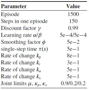
Specifically, the simulation model of the proposed algorithm was established in MATLAB, and a simulation environment was set up. In the real world, the Robot Operating System (ROS) was used to establish communication with the 7-DOF Sawyer manipulator, creating a practical motion environment. The operating system used for training the algorithm is Windows 11, with an i5-12500H CPU and an NVIDIA RTX 4060 Ti GPU. In the experiment, the end-effector of the 7-DOF manipulator needs to move from the initial position to the target position while avoiding obstacles. Table I lists the other parameter settings used in this paper.
Parameter.

Efficiency of distance algorithms.

5.1. Efficiency of distance algorithms
The computational load of the distance algorithm GJK depends on the number of vertices in the 3D models of the two objects, requiring a total of
 $N_{\mathrm{a}}+N_{b}$
operations, where
 $N_{\mathrm{a}}$
and
 $N_{b}$
are the number of vertices in the 3D models of the two objects, respectively. For the case of calculating the distance between the manipulator and obstacles, the total number of operations
 $N=\sum _{i=1}^{m}n_{i}$
can be obtained, where
 $n_{i}$
is the number of operations g between the
 $i$
-th link of the manipulator and the obstacle, and
 $m$
is the number of links. If there are
 $k$
obstacles in the environment, the total number of operations is
 $N_{k}=kN$
. However, this operation only exists in the first iteration of the algorithm, and the subsequent iteration time is an extremely small constant, as shown in refs. [Reference Khan, Li and Luo6, Reference Gilbert, Johnson and Keerthi30, Reference Montanari, Petrinic and Barbieri31]. As shown in Figure 6, we tested the time consumed by the GJK algorithm, AABB algorithm, and Voronoi algorithm to calculate the distance between a single link of the manipulator and an obstacle on a computer. The experiment was conducted 1000 times, and the obstacle contained 32 randomly generated vertices. It can be seen from Figure 6 that the GJK algorithm performs excellently among the three algorithms, with relatively stable computational efficiency, and the calculation time for a single link is controlled at the microsecond level. Even if there are multiple obstacles in the environment, the calculation time is at the millisecond level, which can fully meet the requirements of motion control.
5.2. Network training results
The results after 1500 training epochs for each algorithm are shown in Figure 7. Figure 7(a) shows the training results for the COR_DDPG, DGA_DDPG, and DGA_TD3 algorithms, where the red dashed line indicates the reference line for the increased probability of the algorithm reaching the target position. It can be observed that the DGA_TD3 algorithm significantly outperforms the other two algorithms. Specifically, it has a lower probability of reaching the target position in the early stages of training and achieves the maximum reward value. Additionally, it can stably reach the target position in the middle and later stages of training until it fully converges. Comparing the COR_DDPG and DGA_DDPG algorithms, it is evident that DGA_DDPG outperforms COR_DDPG. COR_DDPG does not converge even at the end of training, whereas DGA_DDPG, although performing poorly in the early stages of training, can converge in the later stages. Figure 7(b) compares the training results of the DGA_TD3 and GA_TD3 algorithms. The curve of the GA_TD3 algorithm indicates that the lack of a decay factor may lead to local optima in the early stages of training. However, in the middle and later stages, it can escape these local optima and successfully reach the target position more stably.
Reward changes during algorithm training.

To provide a more intuitive and clear comparison of the four algorithms, Figures 8 and 9 are supplementary data for Figure 7. Figure 8(a) compares the success rates of the four algorithms over 1500 training epochs. It can be seen from Figure 8(a) that DGA_TD3 has the highest success rate, followed by GA_TD3 and DGA_DDPG, while COR_DDPG has the lowest success rate. In Figure 9, further analysis of the success rates at different stages of the entire training episode can indirectly reflect the convergence speed and convergence ability of the algorithms. DGA_TD3 still leads the other algorithms at different stages, with the trends of the other algorithms being similar to those in Figure 8(a). Figure 8(b) shows the average number of steps per episode for the four algorithms during training. Since the total number of steps per episode is 150, but an episode will end early if the target point is reached, the average number of steps can also reflect the performance of the algorithms. In summary, the performance of the DGA_TD3 algorithm is far superior to the other three algorithms. However, since the training effect of the TD3 algorithm is better than that of the DDPG algorithm, the training effect of the GA_TD3 algorithm, which lacks a decay factor, is somewhat reduced, resulting in similar performance between the GA_TD3 and DGA_DDPG algorithms. The COR_DDPG algorithm has the lowest performance and cannot fully converge. This is because the artificial potential field method is not suitable for scenes with irregular obstacles, and the algorithm itself has certain defects, making it difficult to obtain the correct solution.
Success rate and average steps during algorithm training.

Comparison of success rates at different stages.

5.3. Motion planning and obstacle avoidance analysis
Set the safety threshold distance
 $D_{1}=8\,\text{cm}$
and
 $D_{2}=4\,\text{cm}$
. In this section, the differences in motion paths among the DRL algorithms using the artificial potential field method (COR_TD3) [Reference Liu, Ying, Jiang, Shan and Shen28], the GJK method (DGA_TD3), and the BAORNN algorithm using the GJK algorithm [Reference Khan, Li and Luo6] will be compared. Figures 10 and 11 show the motion planning results of the GJK algorithm and the artificial potential field algorithm, respectively, and Figure 12 presents the motion planning results of the BAORNN algorithm. From the analysis of the motion results in Figure 11, since the artificial potential field method will expand the range of obstacles, the path using the artificial potential field algorithm usually moves away from the obstacles first to obtain a larger reward. However, because the distance between the target position set in the training process and the obstacle is relatively close, the manipulator will be attracted to the target position. As a result, the position of the manipulator’s links is not optimal and may be very close to the obstacle. This is also one of the direct reasons for the poor training effect in the previous section, because contact with the obstacle during training is directly judged as a failure.
Motion planning and obstacle avoidance with DGA_TD3.

Motion planning and obstacle avoidance with COR_TD3 [Reference Liu, Ying, Jiang, Shan and Shen28].

Motion planning and obstacle avoidance with BAORNN [Reference Khan, Li and Luo6].

From the analysis of the motion results in Figure 12, the motion results of the BAORNN algorithm using the GJK method are better than those of the COR_TD3 algorithm. This algorithm ensures that the manipulator does not collide with obstacles, and at the same time, keeps the end effector of the manipulator from being too far away from the target point. However, because the output of this algorithm is the joint position and the step size needs to be adjusted manually, the planned trajectory is not very smooth, and there are multiple cases where the end effector suddenly changes its movement direction. In practical manipulator applications, this will cause abrupt changes in the torque or acceleration of the manipulator joints, which will damage the joints of the manipulator to a certain extent. Comparing the motion planning results in Figure 10, the DGA_TD3 algorithm can plan an efficient and smooth motion trajectory on the premise of ensuring the safety of the manipulator. To sum up, the method proposed in this paper, which integrates the GJK distance algorithm into reinforcement learning, performs better when facing multiple irregular obstacles in the environment.
Algorithm with joint angles output.

Algorithm with joint angular acceleration output.

Figures 13 and 14 show the change curves of the joint information of the manipulator during the motion planning process. Figure 13 is the joint angle as the algorithm output, and Figure 14 is the joint angular acceleration as the algorithm output, both of which use the same TD3 algorithm framework. Considering the real application scenarios of the manipulator, it is necessary to limit the joint information for both algorithms. For the algorithm that uses joint angles as output, the joint angle limit is set to
 $\pm 0.85\pi \,\text{rad}$
, and the joint angular velocity limit is set to
 $\pm 0.024\pi \,\text{rad}\,\text{s}^{-1}$
. For the algorithm that uses joint angular accelerations as output, the joint physical limit mechanism mentioned in this paper is used, with the joint angle limit set to
 $\pm 0.85\pi \,\text{rad}$
, the joint angular velocity limit set to
 $\pm 0.035\pi rad/s$
, and the joint angular acceleration limit set to
 $\pm 0.0015\pi \,\text{rad}\,\text{s}^{-2}$
. In Figures 13(a) and 14(a), it can be seen that the algorithm that uses joint angular accelerations as output has smoother joint angle changes, better meeting the needs of real manipulators. The essence of this phenomenon is whether the torque changes of each joint of the manipulator are stable, i.e., the changes in joint angular acceleration. From Figure 13(c), it is analyzed that the algorithm with joints as outputs produces an abrupt change in angular acceleration during motion, it reaches a large peak, e.g.,
 $\overset{\bullet \bullet }{\theta }_{7}=-0.093\pi \,\text{rad}\,\text{s}^{-1}$
when
 $t=6.5s$
, which will lead to abrupt changes in the output torque. If such situations frequently occur during motion, the manipulator is very likely to be damaged. However, in Figure 14(c), the algorithm that uses joint angular accelerations as output always ensures that the peak value is within a controllable range. Therefore, the latter can greatly reduce the probability of manipulator damage while completing the task. This proves the reliability and advancement of the method used in this paper using joint angular acceleration as the output.
Motion planning for manipulators in real environments.

5.4. Real environment validation
In this section, we will validate the proposed method in this paper using a real manipulator in the real world. The algorithm validation section can be divided into the following points: First, a MATLAB script is used to complete the training of the DRL model in the simulation environment. Second, the kinematics, dynamics model, control law, collision detection algorithm, and other components of the manipulator are encapsulated into an SDK software package and deployed on the Sawyer manipulator. Third, a communication network node is constructed using the ROS, with the network protocol being the TCP/IP protocol, forming a distributed communication network. This network enables real-time communication between the computer and the manipulator, including the computer publishing and subscribing to messages that the manipulator receives to control joint movements; and the manipulator feeding back observational information, allowing the computer to obtain the manipulator’s state and output the next expected action through the trained reinforcement learning model. The system is composed of a remote computer, a local computer of the manipulator, a software operating system (Ubuntu 20), and the ROS1 operating system.
Difference between manipulator and target coordinates.

Changes in joint torque.

Figure 15 shows the motion planning tasks completed by the manipulator driven by the baseline algorithm COR_TD3 (Figure 15(a)) and the proposed DGA_TD3 algorithm (Figure 15(b)), with the motion paths of the manipulator labeled at the corresponding stages. Three-dimensional coordinate differences between the end-effector of the manipulator and the target position were recorded during the motion, as shown in Figure 16. Comparing Figures 16(a) and (b), it is obvious to conclude that the trajectory in Figure 16(a) (COR_TD3) is worse than the trajectory in Figure 16(b) (DGA_TD3). DGA_TD3 can clearly reach the target point more efficiently, while the y-coordinate of COR_TD3 exceeds the given target y-value during the motion, indicating that the manipulator made an unnecessary decision to move away from the target point during the motion. Figure 17 depicts the torque variations of the seven joints during the motion of the manipulator. Specifically, Figure 17(a) illustrates the torque output characteristics of the baseline algorithm COR_TD3 for angle output, which exhibits distinct short-term abrupt changes in torque. In contrast, Figure 17(b) shows that the DGA_TD3 algorithm proposed in this study maintains stable torque throughout the entire motion process, with no significant abrupt changes observed.
Such a difference holds significant implications in practical applications. Taking the Sawyer manipulator used in this study as an example, which is driven by motorized joints, abrupt changes in torque would imply that a large current flows through the motor in a short period. This not only may compromise the operational stability of the manipulator but also pose a risk of causing permanent damage to the joints. Therefore, to summarize, in the real world, the method proposed in this paper can also exhibit better performance than the baseline algorithm.
6. Conclusion
This paper proposes a motion planning scheme for redundant manipulators to avoid obstacles based on a DRL algorithm, considering the actual shapes of obstacles. Starting from the kinematics model of the manipulator, the scheme uses the GJK distance algorithm to obtain the actual distance from obstacles. Based on this distance, a composite reward function for DRL is constructed to complete the obstacle avoidance, path planning, and trajectory planning tasks during the manipulator’s motion. The GJK distance algorithm provides a more accurate and reliable distance from obstacles. The action output of the DRL algorithm is the joint angular acceleration, which avoids complex IK calculations and sudden changes in joint velocity during obstacle avoidance. The designed composite reward function improves the training efficiency of the algorithm and accelerates its convergence time, with a more significant improvement after the introduction of the decay factor. Finally, the feasibility of the scheme is verified on a 7-DOF manipulator in both simulation and real-world environments. Compared with other baseline algorithms, the scheme demonstrates better strategy selection in path planning and trajectory planning. In future work, we will consider the following two aspects: First, after reaching the target point, the velocities and accelerations of all joints of the manipulator will be reduced to 0, which is necessary for multi-task motion in real engineering applications. Second, the dynamics of the manipulator will be combined with the improved kinematics solution proposed in this paper to achieve a complete control process.
Author contributions
Qing Yang: Conceptualization, writing—review and editing. Ju Chen: Investigation, methodology, writing—original draft, and writing—review and editing. Yi Zhang: Validation, visualization. Liang Ge: Funding acquisition. Yun Xiao Wang: Data curation, visualization.
Financial support
This work was supported by the National Natural Science Foundation of China (No. 52374234).
Competing interests
I have nothing to declare. The authors have no relevant financial or non-financial interests to disclose.
Ethical approval
Not applicable.