1. Introduction
The effect of turbulence on the settling velocity of heavy particles, in contrast to settling in quiescent fluids, has long been a focal point of research in turbulent multiphase flows (Balachandar & Eaton Reference Balachandar and Eaton2010). To quantify this effect, we define the modification factor
 $A_c \equiv u_T/u_Q$
, where
 $u_T$
is the average terminal settling velocity in turbulence, and
 $u_Q$
is the terminal velocity in quiescent fluids. It is well established that
 $A_c$
can either exceed or fall below unity, depending on the intricate interactions between particle characteristics and flow properties.
For small particles of weak or moderate inertia,
 $A_c$
typically exceeds 1 due to preferential sweeping (or fast-tracking), in which particles align with downward-moving vortices, enhancing their settling velocity (Maxey Reference Maxey1987; Wang & Maxey Reference Wang and Maxey1993; Aliseda et al. Reference Aliseda, Cartellier, Hainaux and Lasheras2002). This effect is most pronounced at a specific Stokes number
 $St_k \equiv \tau _p/\tau _k$
(the ratio of the particle response time
 $\tau _p$
to the Kolmogorov time
 $\tau _k$
), whose optimal value depends on other parameters such as the settling number
 $S_L = u_Q/u'$
, where
 $u'$
represents the turbulent fluctuation velocity. While the exact peak varies, previous studies generally indicate that preferential sweeping is strongest for
 $St_k \in [0.1, 1]$
, with some data points extending slightly beyond this range (e.g. Wang & Maxey Reference Wang and Maxey1993; Aliseda et al. Reference Aliseda, Cartellier, Hainaux and Lasheras2002; Bec, Homann & Ray Reference Bec, Homann and Ray2014; Good et al. Reference Good, Ireland, Bewley, Bodenschatz, Collins and Warhaft2014; Ireland, Bragg & Collins Reference Ireland, Bragg and Collins2016; Petersen, Baker & Coletti Reference Petersen, Baker and Coletti2019). In this regime, particles preferentially concentrate outside vortices, allowing them to follow descending fluid streams more effectively and thereby accelerating their descent (Yang & Lei Reference Yang and Lei1998; Aliseda et al. Reference Aliseda, Cartellier, Hainaux and Lasheras2002; Yang & Shy Reference Yang and Shy2005).
As particle inertia increases, additional mechanisms such as nonlinear drag and loitering begin to influence particle settling (Nielsen Reference Nielsen1993; Wang & Maxey Reference Wang and Maxey1993). Nonlinear drag arises from the velocity-dependent drag force at finite particle Reynolds numbers, which is intensified by lateral motions and fluctuations in settling velocity (Clift, Grace & Weber Reference Clift, Grace and Weber2013; Byron Reference Byron2015; Fornari et al. Reference Fornari, Picano and Brandt2016a
). Loitering occurs when particles statistically spend longer (or shorter) times in upward (or downward) flow regions during their descent, leading to a reduction in
 $A_c$
(Nielsen Reference Nielsen1993). The competition between preferential sweeping and these decelerating mechanisms determines whether
 $A_c$
exceeds or falls below unity. Specifically, for sub-Kolmogorov particles,
 $A_c \gt 1$
typically occurs when the settling number
 $S_L = u_Q/u'$
is sufficiently small. Conversely, as
 $S_L$
increases,
 $A_c$
tends to drop below unity (Murray Reference Murray1970; Nielsen Reference Nielsen1993; Good et al. Reference Good, Ireland, Bewley, Bodenschatz, Collins and Warhaft2014).
In contrast to the extensive research on sub-Kolmogorov particles, studies examining how turbulence affects the settling velocity of finite-size particles – whose sizes approach or exceed the Kolmogorov length scale – are relatively scarce. Byron (Reference Byron2015) found that the settling velocity of particles larger than the Taylor length scale was reduced by 40–60 % in turbulent conditions for various shapes with
 $S_L\approx 1$
. In contrast, Chouippe & Uhlmann (Reference Chouippe and Uhlmann2015) reported a smaller reduction of only 1.5 % for particles with size 6.7 Kolmogorov length scales at settling number
 $S_L \approx 5.1$
. Fornari et al. (Reference Fornari, Picano, Sardina and Brandt2016b
) investigated the reduction in settling velocity across varying
 $S_L$
values, and noted that the magnitude of the reduction decreases as
 $S_L$
increases. These reductions were primarily attributed to nonlinear drag resulting from the lateral particle motion and fluctuations in the settling velocity. Moreover, studies of fixed particles in turbulent flow have identified small-scale turbulence as a significant factor enhancing momentum exchange across the particle boundary layer, thereby increasing particle drag (Homann, Bec & Grauer Reference Homann, Bec and Grauer2013; Peng & Wang Reference Peng and Wang2023).
Conversely, observations of settling velocity enhancements for finite-size particles typically require specific conditions. For example, Chouippe & Uhlmann (Reference Chouippe and Uhlmann2019) noted that particle clustering could enhance settling, outweighing reduction mechanisms as particle volume fraction increases. Friedman & Katz (Reference Friedman and Katz2002) found that certain above-Kolmogorov-length diesel droplets could rise faster in turbulence than in quiescent water, with droplet deformation likely contributing to this behaviour. Overall, for non-clustering, rigid finite-size particles, reduced settling velocities are the predominant outcome.
Although previous studies have provided valuable insights into the effects of turbulence on the settling velocity of finite-size particles, a critical gap remains: the influence of particle inertia on these effects. It is well established that under the same
 $S_L$
but different
 $St_k$
, sub-Kolmogorov particles exhibit distinct
 $A_c$
values due to the strong dependence of preferential concentration on
 $St_k$
(Wang & Maxey Reference Wang and Maxey1993; Rosa et al. Reference Rosa, Parishani, Ayala and Wang2016). However, for finite-size particles, the impact of particle density ratio under the same settling conditions has not been investigated. It can be anticipated that the heavy particles tend to follow turbulent fluid motions less, and experience weaker fluctuations than light particles, but how this difference affects the settling velocity remains unclear.
Another central question of this study is whether a unified model can be developed to predict
 $A_c$
across a range of particle and flow conditions, encompassing both small and finite-size particles. Previous efforts have focused primarily on sub-Kolmogorov particles, suggesting that
 $A_c \gt 1$
occurs when
 $S_L$
falls below certain thresholds (Nielsen Reference Nielsen1993; Good et al. Reference Good, Ireland, Bewley, Bodenschatz, Collins and Warhaft2014). More sophisticated models that incorporate the particle Froude number and flow Reynolds number have also been proposed to predict the enhancement of settling velocity due to preferential sweeping (Davila & Hunt Reference Davila and Hunt2001; Rosa et al. Reference Rosa, Parishani, Ayala and Wang2016; Petersen et al. Reference Petersen, Baker and Coletti2019). However, none of these models reliably predicts whether
 $A_c \gt 1$
or
 $A_c \lt 1$
for finite-size particles, as existing data from particle-resolved direct numerical simulations (DNS) failed to validate such criteria (Fornari et al. Reference Fornari, Picano and Brandt2016a
).
The remainder of the paper is structured as follows. In § 2, we outline the problem of interest and introduce the parameter settings for the numerical simulations. This section also details the numerical method used to achieve a statistically stationary turbulent field laden with settling particles. In § 3, we conduct a thorough validation of the turbulence generation method, and perform a convergence study on domain size and grid resolution. Section 4 discusses the main findings regarding how particle inertia influences the effects of turbulence on the settling behaviour, as well as efforts to establish a unified model to predict whether turbulence enhances or reduces the settling speed. Finally, we summarise the key conclusions in § 5.
2. Parameter setting and simulation details
2.1. Parameter setting of the simulation cases
When a settling spherical particle reaches its terminal velocity
 $u_Q$
in quiescent fluids, a balance is established between the gravitational forces (i.e. body force and buoyancy force) and drag force. This balance can be expressed as
 \begin{equation} \left (m_p - m_f\right )g = \frac {1}{6}\unicode{x03C0} {d}_p^3 \left (\rho _p - \rho _f\right )g = 3\unicode{x03C0} \rho _f {d}_p \nu u_Q f_D, \end{equation}
where
 $m_p$
and
 $m_f$
are the particle mass and the mass of fluid volume occupied by the particle, respectively,
 ${d}_p$
is the particle diameter,
 $\rho _p$
and
 $\rho _f$
are the particle and fluid densities, respectively,
 $g$
is the gravitational acceleration,
 $\nu$
is the kinematic viscosity of the fluid, and
 $f_D$
is the nonlinear drag correction coefficient.
In non-dimensional form, this equation becomes
 \begin{equation} \frac {u_Q {d}_p}{\nu } = {Re}_Q = \frac {1}{18f_D}\, Ga^2, \end{equation}
where
 ${Re}_Q$
is the particle Reynolds number based on the terminal velocity, and
 $Ga = \sqrt { (\rho _p/\rho _f - 1 )g{d}_p^3/\nu ^2}$
is the Galileo number, which quantifies the relative importance of gravitational and viscous forces. Since
 $f_D$
is also a function of the particle Reynolds number, as expressed by Schiller & Naumann (Reference Schiller and Naumann1933),
 \begin{equation} f_D = 1 + 0.15\,{Re}_Q^{0.687}, \end{equation}
the terminal Reynolds number
 ${Re}_Q$
is determined solely by the Galileo number for a particle settling in quiescent fluids.
For a spherical particle settling in homogeneous isotropic turbulence (HIT), its terminal velocity
 $u_T$
depends not only on the five fundamental parameters –
 $\rho _f$
,
 $\rho _p$
,
 $g$
,
 ${d}_p$
and
 $\nu$
– that dictate the settling velocity in quiescent fluids
 $u_Q$
, but also on two turbulence-related parameters: the ensemble-averaged fluctuation velocity
 $u'$
and the energy dissipation rate
 $\varepsilon$
that characterise HIT. We do not consider the effects of particle shape (Byron Reference Byron2015) or clustering (Chouippe & Uhlmann Reference Chouippe and Uhlmann2019; Petersen et al. Reference Petersen, Baker and Coletti2019) due to particle–particle interactions as we assume that the particle volume fraction is sufficiently low.
Using dimensional analysis, this relationship can be expressed as
 \begin{equation} u_{T} = h\left (\rho _f,\rho _p, g, {d}_p, \nu , u', \varepsilon \right )\quad\rightarrow\quad A_c = \frac {u_T}{u_Q} = h\left (Ga, St_k,S_L, {d}_p^*\right ), \end{equation}
where the four dimensionless parameters introduced are the Galileo number
 $Ga$
(which is interchangeable with
 ${Re}_Q$
), the Stokes number
 $St_k = \tau _p/\tau _k$
that quantifies particle inertia, where
 $\tau _p = \rho _p {d}_p^2/ (18\rho _f\nu )$
is the particle response time, the settling number
 $S_L$
, and the relative particle size
 ${d}_p^* = {d}_p/\eta$
, with
 $\eta = (\nu ^3/\varepsilon )^{1/4}$
representing the Kolmogorov length scale.
In the quiescent fluids, the Galileo number governs the particle’s settling, leaving the other three dimensionless parameters irrelevant. However, under turbulent conditions, the flow around the particle is never steady due to the ambient turbulence, which significantly influences the particle motion. The particle’s response to these turbulent fluctuations impacts its settling process. Previous investigations of drag forces on fixed particles in turbulent flow have demonstrated this effect (Homann et al. Reference Homann, Bec and Grauer2013; Peng & Wang Reference Peng and Wang2023).
A central question driving this study is: how does particle inertia affect settling velocity when the settling effect, quantified by the Galileo number
 $Ga$
, remains constant? It is expected that particles with varying inertia will respond differently to turbulent fluctuations. However, the precise impact of these differences on the particle’s settling speed remains unclear. To explore this, we set up six cases, covering three values of
 $Ga$
(20, 60 and 100) and two distinct density ratios
 $\rho _p/\rho _f = 1.05$
and 51. All cases share the same background turbulence. For the cases with the same value of
 $Ga$
but different density ratios, the value of gravitational acceleration is varied. This variation is not entirely feasible to reproduce in experiments if the sedimentation is driven by gravity, but can be realised if the driving force is due to other types of body forces, such as an electric field or centrifugal force. The choice of a density ratio as high as 51 distinguishes this study from previous research, where the density ratios were typically slightly above unity (Chouippe & Uhlmann Reference Chouippe and Uhlmann2015; Byron Reference Byron2015; Fornari et al. Reference Fornari, Picano and Brandt2016a
,
Reference Fornari, Picano, Sardina and Brandtb
).
The parameters of these cases are summarised in table 1. Under the generated HIT conditions in this study, the three values of
 $Ga$
correspond to settling numbers
 $S_L=0.21$
, 1 and 1.96, encompassing both
 $S_L \lt 1$
and
 $S_L \gt 1$
. For convenience, we refer to particles with the small and large density ratios as light and heavy, respectively. The three
 $Ga$
values will be classified as weak, moderate and strong settling effects in subsequent discussions.
Parameters of cases with identical
 $Ga$
,
 $S_L$
and
 ${d}_p/\eta$
.

In this study, the theoretical particle settling velocity in quiescent fluid,
 $u_Q$
, computed from (2.1)–(2.3), serves as the baseline for terminal settling. However, it is important to note that these values are derived by neglecting the two-way coupling between the particle and the surrounding fluid. Due to the no-slip boundary condition, the fluid around a falling particle is dragged downwards, reducing the slip velocity between the particle and the fluid (see e.g. Figure 7(b) in Chouippe & Uhlmann Reference Chouippe and Uhlmann2019). Consequently, the drag force acting on the particle decreases, leading to a settling velocity higher than
 $u_Q$
.
Recent studies comparing one-way and two-way coupling have demonstrated that particle feedback on turbulence can significantly enhance settling velocity (Monchaux & Dejoan Reference Monchaux and Dejoan2017; Tom, Carbone & Bragg Reference Tom, Carbone and Bragg2022; Bhattacharjee et al. Reference Bhattacharjee, Tom, Carbone and Bragg2024). Unlike these point-particle simulations, the present particle-resolved simulations inherently account for two-way coupling, making it difficult to isolate this effect. However, since our focus is on contrasting particle settling in laminar and turbulent flows, and two-way coupling also exists in laminar cases, differences between these cases primarily reflect the influence of turbulence.
To facilitate comparison, we conducted two laminar cases with light and heavy particles settling in quiescent fluids under strong settling conditions. Under weak and moderate settling effects, previous studies (e.g. Fornari et al. Reference Fornari, Picano, Sardina and Brandt2016b ) have shown a significant reduction in settling velocity compared to laminar cases. Since these reductions are too large to be solely attributed to differences in two-way coupling between turbulent and laminar flows, we omit those cases to conserve computational resources.
2.2. Simulation method
The simulations in this study utilised the lattice Boltzmann method with the interpolated bounce-back schemes to ensure second-order accuracy in the no-slip boundary treatment on particle surfaces. This method has been applied previously to simulate both homogeneous and wall-bounded particle-laden turbulent flows (e.g. Peng et al. Reference Peng, Sun and Wang2023, Reference Peng, Wang and Chen2024).
To investigate how turbulence affects particle settling velocity, the ideal approach would be to release a single particle randomly into the flow, and track its velocity over a sufficiently long period to minimise statistical uncertainties. However, this approach demands extensive simulation time, and significantly increases computational costs. Instead, we released multiple particles into the flow to enhance the sample size for statistical analysis. While particle–particle interactions can influence terminal settling velocity compared to isolated particles (Fornari et al. Reference Fornari, Picano and Brandt2016a
), we maintained a low particle volume fraction
 $\phi _p = 0.1\,\,\%$
to approximate isolated particle behaviour.
To further mitigate the effects of particle–particle interactions, we excluded all data samples where another particle was within a cut-off distance
 $d_{ij} = 2{d}_p$
, where
 $d_{ij}$
is the centre-to-centre distance between two particles. While the choice of this cut-off is not based on a rigorous physical criterion, it effectively removes data points influenced by particle–particle collisions, direct short-range hydrodynamic interactions, and some of their residual effects. Particle–particle interactions were modelled using a normal lubrication force and a soft-sphere collision model, which accounts for both normal and tangential collision forces. This approach was described and validated in our recent work (Peng, Wang & Chen Reference Peng, Wang and Chen2024).
To simulate HIT with periodic boundaries under the influence of gravity, we solve the Navier–Stokes equation with a modified pressure
 $\tilde {p} \equiv p -\rho _f g ( \boldsymbol{x} \boldsymbol{\cdot} \,\hat {\!\boldsymbol{j}})$
, which is the actual pressure
 $p$
minus the hydrostatic pressure
 $ \rho _f g ( \boldsymbol{x} \boldsymbol{\cdot} \,\hat {\!\boldsymbol{j}})$
(where
 $\boldsymbol{x}$
is the spatial coordinate, and
 $\,\hat {\!\boldsymbol{j}}$
denotes the direction of gravity). The Navier–Stokes equation becomes
 \begin{equation} {\partial }_t\left (\rho _f \boldsymbol{u}\right ) + \boldsymbol{\nabla} \boldsymbol{\cdot} \left (\rho _f \boldsymbol{u} \boldsymbol{u}\right ) = -\boldsymbol{\nabla} \tilde {p} + \boldsymbol{\nabla} \boldsymbol{\cdot} \boldsymbol{\Pi } . \end{equation}
where
 $\boldsymbol{u}$
is the fluid velocity, and
 $\boldsymbol{\Pi }$
is the viscous stress tensor. Since the gravitational body force is absorbed into the modified pressure
 $\tilde {p}$
, no explicit body force is applied to the flow field. Due to the fact that the interpolated bounce-back scheme is used to directly handle the no-slip boundary condition on the particle surface, no artificial two-way coupling force is needed in (2.5) to reflect the feedback effects of particles in the fluid phase. Meanwhile, the governing equation for the translational velocity
 $\boldsymbol{v}$
of a particle must be modified to account for the use of
 $\tilde {p}$
as
 \begin{equation} m_p\frac {{\textrm d} \boldsymbol{v}}{{\textrm d}t} = \oint _{\partial S}{\left (-p\boldsymbol{I} + \boldsymbol{\Pi }\right )\boldsymbol{\cdot} \boldsymbol{n}\, {\textrm d}S} + m_p g \,\hat {\!\boldsymbol{j}} = \oint _{\partial S}{\left (-\tilde {p}\boldsymbol{I} + \boldsymbol{\Pi }\right )\boldsymbol{\cdot} \boldsymbol{n}\, {\textrm d}S} + \left (m_p - m_f\right ) g \,\hat {\!\boldsymbol{j}}. \end{equation}
That is, the last term on the right-hand side of (2.6) now represents the gravitational body force minus the buoyancy force (part of the hydrodynamic force from the carrier fluid). This term is implemented as an external force in the simulations.
Given that the background turbulent flow employs periodic boundary conditions in all three directions, there is no mechanism to counteract this external force, leading to a continuous increase in the mean velocity of the particle–fluid system. To prevent the mean system velocity from evolving indefinitely, we regularly apply a Galilean transformation to both the fluid and particle velocities. At set intervals, we compute the mean fluid velocity in the settling direction
 $\langle v_f\rangle ^s$
, and subtract it from the velocities of both fluid and particles. This adjustment preserves the relative velocity between the fluid and particles, and does not affect turbulent fluctuating quantities; it merely ensures that the fluid phase maintains a zero mean velocity, thereby establishing a statistically stationary state for data collection. To optimise computational efficiency, the Galilean transformation is applied every 100 time steps, keeping
 $\langle v_f\rangle ^s$
to approximately
 $0.01\,\%$
of laminar terminal velocity
 $u_Q$
.
Subtracting
 $\langle v_f\rangle ^s$
from the particle velocity is equivalent to applying an impulsive force to the particles, which modifies the force balance equation to
 \begin{equation} \left (m_p - m_f\right )g = \langle F_{D}\rangle = \langle F_{HI}\rangle + \langle F_D^{\prime}\rangle , \end{equation}
where
 $\langle F_D\rangle$
represents the time-averaged drag force acting on the particle,
 $\langle F_{HI}\rangle$
is the hydrodynamic interaction force computed from the simulations, and
 $\langle F_D^{\prime}\rangle$
is defined as
 \begin{equation} \langle F_D^{\prime}\rangle = m_p \frac {\langle v_f\rangle ^{s}}{n\,\Delta t}. \end{equation}
In this equation,
 $n\Delta t$
denotes the time interval between successive corrections. This force balance serves as an indicator of when the particles have reached their terminal settling velocity. Once this state is achieved, fluid and particle statistics are collected over a sufficiently long period to ensure reliable results.
3. Method validation and choices of the computational domain size and grid resolution
3.1. Validation on the background HIT in cuboid domains
The background turbulence in this study is a sustainable HIT, generated by random large-scale forcing in a periodic domain. A potential issue arises: a settling particle may interact with its own wake upon re-entering the domain through the periodic boundary, potentially introducing errors in the measurement of its settling velocity. To mitigate this, we extend the domain size in the settling direction (denoted as the
 $y$
-axis, and the gravity points to the negative
 $y$
direction).
Turbulence is generated using the classic stochastic forcing method of Eswaran & Pope (Reference Eswaran and Pope1988), which applies forcing to the same wavelengths in Fourier space across all three directions to ensure isotropy. This approach is consistent with previous studies (e.g. Fornari et al. Reference Fornari, Picano, Sardina and Brandt2016b
; Chouippe & Uhlmann Reference Chouippe and Uhlmann2019). Once the background turbulence reaches a statistically stationary state, we collect data over an extended period
 $T_{ave}$
for time averaging.
Some previous studies have suggested that reliable turbulent statistics require
 $T_{ave} \geqslant 100 u'^2/\varepsilon$
, where
 $u'^2/\varepsilon$
is the large-eddy turnover time (Tom et al. Reference Tom, Carbone and Bragg2022; Bhattacharjee et al. Reference Bhattacharjee, Tom, Carbone and Bragg2024). However, we argue that a more direct criterion is to quantify the uncertainty of the mean value to ensure sufficient data sampling. To this end, we provide uncertainty estimates wherever possible. Since the flow and particle states at any given time are influenced by their prior evolution – rendering successive samples statistically correlated – the uncertainty of ensemble-averaged quantities (denoted by ‘
 $\pm$
’) is computed as 1.96 times the standard error of the mean to represent a 95 % confidence interval. Specifically, the uncertainty is given by
 $1.96\sigma _{mean}$
, where
 $\sigma _{mean} = \sigma _A\sqrt {2T_c/T_{ave}}$
,
 $\sigma _A$
is the standard deviation of the time series of phase-averaged quantities, and
 $T_c$
is the decorrelation time defined as the lag at which the autocorrelation function drops to 0.5 (see Eswaran & Pope Reference Eswaran and Pope1988; Wang et al. Reference Wang, Ayala, Gao, Andersen and Mathews2014).
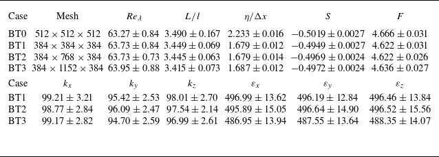
The statistics of the background turbulence are summarised in table 2. These approximately equivalent distributions of the turbulent kinetic energy and dissipation rate associated with each velocity component indicate that the background turbulence remains isotropic. Additionally, the findings from two different grid resolutions,
 $384^3$
and
 $512^3$
, are nearly identical, even for the high-order statistics such as skewness and flatness of longitudinal velocity gradient. This suggests that a grid resolution
 $2\unicode{x03C0} = 384\,\Delta x$
(which translates to
 $\eta /\Delta x \approx 1.7$
and
 $k_{max}\eta \approx 5.7$
, where the largest wavenumber
 $k_{max}$
is approximately half the grid number) is sufficient to resolve turbulent eddies up to the Kolmogorov length scale for the current Reynolds number. The ratio between the domain length
 $L$
and the pseudo-integral length scale
 $l = u'^3/\varepsilon$
is approximately 3.4. Regarding the longitudinal integral length scale
 $l_{11} = \int _0^{\infty } Q_{11}(r)\,{\rm d}r$
, where
 $Q_{11}$
is the longitudinal autocorrelation, we find
 $L/l_{11}\approx 5.7$
. While some studies recommend
 $L/l_{11} \gt 6$
for capturing large-scale structures (e.g. O’Neill et al. Reference O’Neill2004), it is generally accepted that
 $L/l_{11} \gt 4$
provides adequate large-scale resolution, a criterion that our simulations satisfy.
Statistics of the background HIT simulations with different computational domains. In the top panel,
 ${Re}_\lambda$
is the Reynolds number based on the Taylor microscale
 $\lambda = \sqrt {15\nu {u'}^2/\varepsilon }$
,
 $L/l$
is the ratio between the domain size and the integral length scale
 $l = {u'}^3/\varepsilon$
,
 $\eta /\Delta x$
is the ratio between the Kolmogorov length and the grid spacing, and
 $S$
and
 $F$
are the skewness and flatness of the longitudinal velocity gradient, respectively. The bottom panel gives the turbulent kinetic energy and dissipation rate contributed by each velocity component. All the dimensional quantities are scaled with
 $L = 2\unicode{x03C0}$
and
 $\nu = 0.0945$
.

3.2. Validation on the choice of domain length
Next, we justify the choice of domain length in the simulations of particles settling in HIT by setting up three simulations with domain sizes
 $L_x:L_y:L_z = 1:1:1$
,
 $1:2:1$
and
 $1:3:1$
, as illustrated in figure 1. All simulations are conducted with grid resolution
 $L_x/\Delta x = 384$
and
 ${d}_p/\Delta x = 24$
, density ratio
 $\rho _p/\rho _f = 1.05$
, particle volume fraction
 $\phi _p = 0.1\,\%$
, and
 $Ga = 100$
. The particle counts for the three cases are 8, 16 and 24, ensuring consistent particle volume across different configurations.
The HIT with settling particles in domain with different lengths. The isosurfaces represent the vortex structures identified from the Q-criterion, which are coloured by velocity magnitude.

The particle statistics for each simulation are compiled in table 3. These statistics are gathered after the particles have reached their terminal settling velocity over a sufficient duration, ensuring that the balance represented by (2.7) is achieved, with the relative difference between the two sides of the equation not exceeding 0.1 %. Since the particle data collected at each sampling time are temporally correlated and thus cannot be treated as statistically independent, the uncertainties of individual particle statistics are estimated using the same methodology applied to flow statistics as detailed in § 3.1. The uncertainty associated with ensemble-averaged quantities reported in table 3 and subsequent tables is then computed as
 \begin{equation} {\mathrm d}\bar {a} = \sqrt {\frac {1}{N_p^2} \left [ \sum _{i=1}^{N_p} {\mathrm d}a_i^2 + {2T_c\over T_{ave}} \sum _{i=1}^{N_p} \left ( \mu _i - \mu _{ {ensemble}}\right )^2 \right ] } \approx \sqrt {\frac {1}{N_p^2} \sum _{i=1}^{N_p} {\mathrm d}a_i^2 } , \end{equation}
where
 ${\rm d}a_i$
denotes the uncertainty of the time-averaged quantity for the
 $i$
th particle (namely, 1.96 times the standard error),
 ${\rm d}\bar {a}$
is the aggregated uncertainty, and
 $N_p$
is the total number of particles. This approach is applied consistently to all particle statistics presented in this study. The prefactor is
 $1/N_p^2 = (1/N_p)\times (1/N_p)$
, with the first
 $(1/N_p)$
representing averaging of the squared uncertainty, and the second
 $(1/N_p)$
converting the squared uncertainty of the individual particle to that for the ensemble particle average. The correction term involving the difference between the mean of the individual particle data
 $\mu _i$
and the ensemble mean
 $\mu _{{ensemble}}$
was found to be negligible.
Settling particle statistics with different domain lengths: the mean settling velocity, the r.m.s. velocity of the particle in the
 $x$
,
 $y$
and
 $z$
directions, respectively, and the mean slip velocity between the particles and their surrounding fluids projected onto the
 $x$
,
 $y$
and
 $z$
directions, respectively, computed by the Kidanemariam et al. (Reference Kidanemariam, Chan-Braun, Doychev and Uhlmann2013) method. All the particle velocity results have been normalised by
 $u_Q$
.

We denote fluid and particle velocities as
 $\boldsymbol{u}$
and
 $\boldsymbol{v}$
, respectively. Unless specified otherwise, all particle velocity results are normalised by the terminal settling velocity in quiescent fluids,
 $u_Q$
, obtained using the Schiller–Naumann correlation, as computed from (2.2).
As shown in table 3, even a cubic domain is sufficient to contain the particle wake, and ensures that the statistics of particle motion are not affected by the periodic boundary condition in the settling direction. This sufficiency arises because turbulence fluctuations enhance the momentum exchange between the particle wake and the surrounding fluids, while also extending the low-pressure region around the trailing edge of the particle. Both factors help the velocity in the particle wake to restore more quickly to its undisturbed value (Homann et al. Reference Homann, Bec and Grauer2013; Peng & Wang Reference Peng and Wang2023). Consequently, particle wakes in turbulent flows are much shorter than those in laminar flows. However, some persistent wakes may occasionally propagate over long distances due to turbulent intermittency.
For added safety, we will use a domain length ratio
 $L_y/L_x = 2$
in the simulations of particles settling in HIT. In addition to the turbulent cases, we will also simulate particles settling in quiescent fluids as contrast groups. The domain length in these cases is further extended to
 $L_y/L_x = 3$
, as the laminar particle wakes are generally more extended. To further support this choice, we show the contours of ensemble-averaged vorticity
 $\omega _{x} = \partial _{y}w - \partial _{z}v$
on a
 $y$
–
 $z$
plane across the particle centre in figure 2 for the turbulent and laminar cases with
 $Ga = 100$
. The wake structures are well contained in the chosen domain. It is also important to note that this conclusion is based on the case with
 $Ga = 100$
, the highest
 $Ga$
investigated in this study. Since the lengths of the particle wakes decrease as
 $Ga$
reduces, these choices of domain lengths should be more than sufficient for cases with lower
 $Ga$
.
Contours of averaged vorticity in turbulent and laminar cases: (a) case C1 and (b) case L1.

3.3. Validation on the choice of particle resolution
Finally, we validate the choice of particle resolution necessary to accurately resolve the flow around particles and particle motion. In previous studies (e.g. Peng, Ayala & Wang Reference Peng, Ayala and Wang2019; Peng & Wang Reference Peng and Wang2023), we tested uniform flow passing over a fixed sphere, and found that grid convergence was established at
 ${d}_p/\Delta x = 24$
for particle Reynolds number up to 400. This relatively low requirement for particle resolution is likely due to the no-slip boundary treatment of our method, which ensures a second-order-accurate velocity field, as confirmed by various studies (e.g. Peng et al. Reference Peng, Ayala and Wang2019). For the maximum investigated
 $Ga = 100$
in the present study, the terminal Reynolds number of a particle settling in quiescent fluid is
 ${Re}_Q \approx 113.9$
. Therefore, a particle resolution
 ${d}_p/\Delta x = 24$
should be sufficient to accurately capture the mean settling velocity of particles and most instantaneous fluctuations.
To further support this conclusion, we conducted three simulations with different particle resolutions,
 ${d}_p/\Delta x = 16$
, 24, 32. For these cases, the computational domain length ratio was set to
 $L_y/L_x = 2$
, and the mesh size was expanded accordingly to maintain the same ratio of 16 between the domain size and the particle diameter, i.e.,
 $L_x/{d}_p = 16$
. The density ratio was
 $\rho _p/\rho _f = 1.05$
, the volume fraction was
 $\phi _p = 0.1\,\%$
, and
 $Ga$
was set to 100. In figure 3, we present the probability distribution functions (PDFs) of the particle slip velocity computed using the method proposed by Kidanemariam et al. (Reference Kidanemariam, Chan-Braun, Doychev and Uhlmann2013). Despite slight discrepancies due to insufficient sampling, the results from different particle resolutions align closely with one another. The particle statistics are compiled in table 4, indicating that grid convergence is approximately achieved at
 ${d}_p/\Delta x = 16$
.
The PDFs of particle slip velocity in (a) the
 $x$
direction, (b) the
 $y$
direction, and (c) the
 $z$
direction, with various particle resolutions. The red, blue and black curves in each plot represent the results with
 ${d}_p/\Delta x = 16$
,
 $24$
and
 $32$
, respectively.


Based on the validation tests conducted, we will use a mesh
 $384\times 768\times 384$
with
 ${d}_p/\Delta x = 24$
for the simulations of particles settling in HIT. For the contrasting group of particles settling in quiescent fluids, we will utilise an extended computational domain
 $384\times 1152\times 384$
while maintaining the same particle resolution.
4. Results and discussion
Due to the coupling effects between finite-size particles and the turbulence field, the turbulence modified by the presence of particles can, in turn, affect particle motion. Therefore, before contrasting the settling processes of particles with different inertia, it is essential to ensure that the turbulence field remains relatively consistent. Given that the particle volume fraction is kept low at 0.1 %, most turbulence statistics are only marginally affected, as confirmed in table 5, with the exception of the sensitive flatness of the longitudinal velocity gradients. Notably, the two turbulence-related dimensionless parameters – the settling number
 $S_L$
and the relative particle size
 ${d}_p^*$
– remain roughly constant across different cases, as
 $u'$
and
 $\eta$
are only marginally altered by particles. Consequently, any changes in particle settling are attributed to the differences in
 $St_k$
, which quantifies the particle inertia.
Flow statistics in particle-laden cases. The items in this table are identical to those in table 2, with one extra column showing
 $\langle \omega ^2 \rangle \equiv \langle \boldsymbol{\omega }\boldsymbol{\cdot} \boldsymbol{\omega }\rangle$
, where
 $\boldsymbol{\omega } = \boldsymbol{\nabla} \times \boldsymbol{u}$
is the vorticity. All the dimensional quantities are scaled with
 $L = 2\unicode{x03C0}$
and
 $\nu = 0.0945$
.

Although the uncertainties of the statistics are given, to provide direct assessment on the length of the data collecting period
 $T_{ave}$
, we show the time evolution of individual and averaged particle velocity for each turbulent case in figure 4. Each coloured curve represents the time-dependent settling velocity of an individual particle, and the black curve represents the averaged value over different particles. The simulation times are normalised by the particle time scale
 ${d}_p/u'$
, and large-eddy turnover time
 $u'^3/\varepsilon$
, where
 $u'$
and
 $\varepsilon$
use the corresponding values in the unladen single phase case.
Time evolution of individual and averaged particle settling velocity in each turbulent case, for (a–f) representing cases A1, A2, B1, B2, C1 and C2, respectively.

4.1. The effects of particle inertia on the particle velocity
The mean and root mean square (r.m.s.) values of particle velocity for each case are presented in table 6, along with corresponding results for particles settling in quiescent fluids for comparison.
Statistics of particle settling velocity and r.m.s. velocity.

In the laminar cases, the mean settling velocities closely match the analytical predictions from the Schiller–Naumann correlation. This agreement arises from the balance of two competing mechanisms. The first is the intrinsic two-way coupling effect of finite-size particles, which enhances settling (Monchaux & Dejoan Reference Monchaux and Dejoan2017; Tom & Bragg Reference Tom and Bragg2019; Bhattacharjee et al. Reference Bhattacharjee, Tom, Carbone and Bragg2024). As the ambient fluid is also driven downwards by the settling particle, the actual slip velocity between the particle and the disturbed flow is reduced. This, in turn, decreases the drag force acting on the particle, allowing it to achieve a higher settling velocity. The second mechanism is the reduction in settling due to nonlinear drag and local hindering effects from occasional particle–particle interactions (Yin & Koch Reference Yin and Koch2007; Fornari et al. Reference Fornari, Picano, Sardina and Brandt2016b ). Although the particle number in the present study is low, instances of ‘draft-kissing-tumbling’ motion occasionally bring particles into proximity. A group of steadily settling nearby particles experiences increased drag due to long-range hydrodynamic interactions, known as the hindering effect (Richardson & Zaki Reference Richardson and Zaki1954; Peng & Wang Reference Peng and Wang2023). Additionally, particle–particle interactions prevent the r.m.s. velocities in laminar cases from reaching zero, thereby amplifying nonlinear drag.
At higher particle volume fractions, the hindering effect and nonlinear drag can outweigh the settling enhancement from two-way coupling, leading to a reduction in the average settling velocity (Di Felice Reference Di Felice1999; Fornari et al. Reference Fornari, Picano and Brandt2016a ). However, if particles form clusters, then the stronger two-way coupling effect can reverse this trend and enhance settling velocity (Chouippe & Uhlmann Reference Chouippe and Uhlmann2019).
On the other hand, particle velocities in the turbulent cases are significantly lower than
 $u_Q$
, regardless of whether the settling number
 $S_L$
is less than or greater than unity. The smaller
 $S_L$
, the greater the relative reduction in settling velocity. These observations are consistent with findings from other fully resolved simulations (e.g. Fornari et al. Reference Fornari, Picano, Sardina and Brandt2016b
).
It is important to note that the two competing mechanisms that nearly balance in the laminar cases are also present in turbulent cases. Therefore, the significantly reduced settling velocities are more likely driven by particle–turbulence interactions. The discrepancies between these results and the criterion proposed by Good et al. (Reference Good, Ireland, Bewley, Bodenschatz, Collins and Warhaft2014) (
 $A_c \gt 1$
when
 $S_L \lt 1$
, and vice versa) highlight the significant role of finite-size effects in particle settling behaviour.
For small-inertia particles with diameters much smaller than the Kolmogorov length, all turbulence scales effectively act as large scales. A recent study further categorises these large scales into two groups: (i) very large scales above a threshold
 $l_c$
, which have minimal influence on settling velocity as they appear nearly steady from the particle’s perspective; and (ii) scales below this threshold, which play a crucial role in preferential sweeping (Tom & Bragg Reference Tom and Bragg2019). While other parameters, such as
 $St_k$
, can influence the relative importance of settling enhancement and reduction mechanisms, it remains reasonable to infer that their qualitative balance is primarily characterised by the single non-dimensional parameter
 $S_L$
.
In contrast, for finite-size particles – particularly those with diameters significantly larger than the Kolmogorov length – a substantial portion of the turbulence spectrum falls below the particle size. This fundamental difference leads to a qualitatively distinct particle–turbulence interaction compared to point particles. For instance, preferential sweeping becomes less effective due to size-filtering effects (Qureshi et al. Reference Qureshi, Bourgoin, Baudet, Cartellier and Gagne2007; Teixeira & Mériaux Reference Teixeira and Mériaux2022). In such cases, both large and sub-diameter scales contribute to an effective drag enhancement: large scales introduce nonlinear drag, while small scales interact with the particle boundary layer, altering fluid–particle momentum and energy exchange (Peng & Wang Reference Peng and Wang2023). This interplay results in consistently reduced settling velocities.
However, it is important to acknowledge that due to computational cost limitations, the present study is restricted to relatively low Reynolds numbers, where the separation between large and small turbulent scales is not fully developed. It is reasonable to suspect that in sufficiently strong turbulence, finite-size particles might behave more like point particles and experience downward sweeping by very large vortices. While this hypothesis warrants further investigation, it lies beyond the scope of the present study.
Across all
 $Ga$
, the r.m.s. values of particle velocities decrease significantly with increasing particle inertia. At low
 $Ga$
, turbulence fluctuations can still drive particles upwards against gravity, but the probability of upward motion decreases as
 $Ga$
and
 $\rho _p/\rho _f$
increase. Particle inertia also influences the isotropy of the particle velocity fluctuations. The last column of table 6 quantifies this anisotropy with
 $A_{\it{iso}} = (\langle \boldsymbol{v}\boldsymbol{\cdot} \boldsymbol{ e}_x\rangle _{\it{rms}} \langle \boldsymbol{v}\boldsymbol{\cdot} \boldsymbol{e}_y\rangle _{\it{rms}} )^{0.5}/\langle \boldsymbol{ v}\boldsymbol{\cdot} \boldsymbol{e}_y\rangle _{\it{rms}}$
. Nearly isotropic fluctuations are observed for light particles, with
 $A_{\it{iso}}$
values 0.994, 1.004 and 1.060 for the three
 $Ga$
values investigated. For comparison, Fornari et al. (Reference Fornari, Picano, Sardina and Brandt2016b
) reported
 $A_{\it{iso}}$
values 1.03, 1.05 and 1.34 for
 $Ga = 20$
,
 $60$
and
 $145$
, with very light particles (
 $\rho _p/\rho _f = 1.00035$
,
 $1.0034$
and
 $1.020$
). For heavy particles with greater inertia, fluctuations in the settling direction become more pronounced than in the lateral directions, a trend also observed in the laminar cases.
In contrast to the significant variations in particle r.m.s. velocities with increasing inertia, the mean settling speed exhibits only minor changes, particularly under weak and moderate settling effects. However, at sufficiently high
 $Ga$
, particle inertia has a more pronounced impact on mean settling speed. For instance, at
 $Ga = 100$
, the mean settling speed of heavy particles (
 $\rho _p/\rho _f = 51$
) is noticeably lower than that of lighter particles. It is important to note that these observations are made while accounting for the uncertainties in the mean results. As shown in figure 4, under weak settling effects (cases A1 and A2), fluctuations in particle settling velocity are so pronounced that they can obscure the mean value. Reducing these uncertainties would require simulations to run for impractically long durations. Increasing the number of particles could also help to reduce uncertainties; however, increasing the particle count would lead to more frequent particle–particle interactions. This, in turn, would shift the focus away from our objective of investigating how turbulence affects the settling velocity of isolated particles.
Figure 5 shows the PDFs of particle velocity for each case. Since particle motion in the two directions perpendicular to the settling direction is statistically homogeneous, we project the velocity onto the lateral plane, defined by
 $\boldsymbol{e}_{l} = (1,0,1)$
, and the settling direction,
 $\boldsymbol{e}_{s} = (0,1,0)$
, to reduce the number of subplots in the figure.
The PDFs of particle velocity projected to the (a,c,e,g) lateral and (b,d,f,h) settling directions, for (a,b) cases A1 and A2, (c,d) cases B1 and B2, (e,f) cases C1 and C2, and (g,h) cases L1 and L2. Symbols in each plot represent the simulation results, and the corresponding lines show the Gaussian distributions using the means and standard deviations of the simulation data.

In all turbulence cases, the particle velocity fluctuations in both directions are nearly Gaussian. In contrast, the fluctuations in the laminar cases deviate from Gaussian distributions, exhibiting long tails, which are more pronounced for heavy particles. As noted by Fornari et al. (Reference Fornari, Picano and Brandt2016a
), these off-Gaussian distributions could originate from particle–particle interactions. To isolate this effect, we excluded data points where another particle’s centre was within
 $\vert d_{ij}\vert \leqslant 2{d}_p$
, ensuring that directly interacting particles were not considered. Interestingly, when these excluded points were included, the PDFs in the turbulent cases remained largely unchanged. However, as shown in figure 6, the PDFs in the two laminar cases exhibited slightly more pronounced tails, particularly for the settling velocity in the light particle case. This contrast suggests that the long tails in the laminar cases are at least partially attributable to particle–particle interactions. For heavy particles with greater inertia, the influence of past particle–particle interactions persists longer, meaning that even after excluding data points below the
 $\vert d_{ij}\vert = 2{d}_p$
threshold, their impact is still evident. In contrast, the absence of such long tails in the turbulent cases suggests that turbulence dominates the velocity fluctuations, effectively diminishing the role of particle–particle interactions.
The PDFs of the two laminar cases with and without excluding the data points where another particle’s centre was within
 $\vert d_{ij}\vert \leqslant 2{d}_p$
: (a) lateral velocity, (b) settling velocity.

One of the most distinguishing features of finite-size particles, compared to sub-Kolmogorov point particles, is their ability to significantly disturb the surrounding fluids. Thus stronger particle fluctuations do not always lead to greater slip velocities
 $\vert \boldsymbol{u} - \boldsymbol{ v}\vert$
between particles and their ambient fluids. Determining the precise slip velocity for finite-size particles is challenging, as the undisturbed fluid velocity
 $\boldsymbol{u}$
cannot be obtained easily due to the disturbance caused by the particles. We adopt the method proposed by Kidanemariam et al. (Reference Kidanemariam, Chan-Braun, Doychev and Uhlmann2013), which calculates the slip velocity as the difference between the particle velocity
 $\boldsymbol{v}$
and the averaged flow velocity on a concentric shell at distance
 $1.5{d}_p$
from the particle centre. The statistics of the slip velocity are presented in table 7. Although light particles exhibit greater velocity fluctuations, their slip velocity relative to the ambient fluid is not correspondingly amplified. This highlights a key difference between sub-Kolmogorov-scale point particles and finite-size particles, significantly reducing the influence of particle inertia on the settling velocity of finite-size particles, as shown in table 6. When the settling effect is weak, heavy particles tend to have larger slip velocities than light particles because their greater inertia prevents them from closely following the surrounding fluid. However, as
 $Ga$
increases, the slip velocity in the settling direction becomes dominant. Consequently, the reduced settling velocity of heavy particles leads to smaller slip velocities compared to light particles.
Statistics of particle slip velocity.

Although tests for particles settling in quiescent fluids were not conducted for cases with weak and moderate settling effects, the magnitude of slip velocity
 $\langle \vert (\boldsymbol{u} - \boldsymbol{v} )\vert \rangle$
should approximate unity when normalised by
 $u_Q$
, similar to the corresponding heavy particle cases. In these cases, turbulence enhances lateral particle motion, leading to greater slip velocities compared to laminar conditions. However, as
 $Ga$
increases, the settling component becomes the dominant contributor to slip velocity. The reduced settling velocities in turbulent cases then result in lower overall slip velocities, despite turbulence continuing to enhance lateral slip velocity.
The PDFs of componentwise slip velocities in the turbulent cases are shown in figure 7. As before, we project the slip velocity onto the lateral plane and the settling direction. In the lateral plane, the distributions remain Gaussian for all examined
 $Ga$
and
 $\rho _p/\rho _f$
, as expected, since particles do not exhibit preferential motion in a homogeneous and isotropic plane. However, in the settling direction, light particles under moderate and strong settling effects show deviations from Gaussian distributions, with a slightly increased probability of slip velocities exceeding the mean. This trend suggests the presence of a weak loitering effect, where particles spend more time in upward flows than in downward flows (Nielsen Reference Nielsen1993), leading to a higher frequency of above-average slip velocities. Under weak settling effects, turbulence dominates particle motion, reducing the influence of gravitational sedimentation and making the loitering effect less pronounced. Likewise, for heavy particles with significant inertia, turbulence has a weaker influence on their motion, resulting in the absence of loitering.
The PDFs of the slip velocity computed with the Kidanemariam et al. (Reference Kidanemariam, Chan-Braun, Doychev and Uhlmann2013) approach.

4.2. The effects of particle inertia on the hydrodynamic force
Previous studies have focused on analysing nonlinear drag to understand turbulence’s effects on particle settling velocities (Byron Reference Byron2015; Fornari et al. Reference Fornari, Picano, Sardina and Brandt2016b
). The nonlinear drag
 $F_D^{\it{NL}}$
can be expressed as
 \begin{equation} F_D^{\it{NL}} = C_D\frac {1}{8}\rho _f \unicode{x03C0} {d}_p^2\, \vert \boldsymbol{u} - \boldsymbol{v}\vert \left (\boldsymbol{u} - \boldsymbol{ v}\right )\boldsymbol{\cdot} \boldsymbol{e}_y, \end{equation}
where the drag coefficient
 $C_D$
for moderate
 ${Re}_p$
is well captured well by the Schiller–Naumann correlation (Schiller & Naumann Reference Schiller and Naumann1933)
 \begin{equation} C_D = \frac {24}{{Re}_p}\left (1+0.15\,{Re}_p^{0.687}\right ) = \frac {24\nu }{{d}_p\,\vert \boldsymbol{u} - \boldsymbol{v}\vert }\left [1 + 0.15\left (\frac {{d}_p\,\vert \boldsymbol{u} - \boldsymbol{v}\vert }{\nu }\right )^{0.687}\right ]. \end{equation}
Under this correlation,
 $F_D^{\it{NL}}$
becomes a nonlinear function of the slip velocity
 $\vert \boldsymbol{u} - \boldsymbol{ v}\vert$
. In turbulent conditions, a settling particle experiences lateral motions, and its settling velocity fluctuates, both of which enhance
 $F_D^{\it{NL}}$
and statistically lead to smaller settling velocities. In the study by Fornari et al. (Reference Fornari, Picano, Sardina and Brandt2016b
), the change of nonlinear drag due to lateral motions was termed the ‘cross-flow velocity’, while the effect of fluctuating settling velocity was referred to as ‘nonlinear-induced drag’. Here, we combine these mechanisms under the umbrella of nonlinear drag effects without further decomposition.
Using the previously obtained samples of slip velocity, we can compute the nonlinear drag directly. The results are summarised in table 8, where all the forces are normalised by the gravitational force
 $G = (m_p - m_f)g$
in each case. For particles with
 $Ga = 20$
, the mean values of
 $\langle F_{D}^{\it{NL}}\rangle$
are approximately 0.68, which increases to
 $0.72$
and
 $0.78{-}0.83$
when
 $Ga$
increases to 60 and 100, respectively. In comparison, the nonlinear drag accounts for 92–96 % of the total drag in the laminar cases. These findings are consistent with the results reported by Fornari et al. (Reference Fornari, Picano, Sardina and Brandt2016b
), where under
 $Ga = 100$
, the nonlinear drag contributed to 86 % and 94 % in the turbulent and laminar cases, respectively.
Statistics of nonlinear drag and actual drag, and the contributions from the pressure and viscous stresses to the actual drag, denoted as
 $F_D^p$
and
 $F_D^{v}$
, respectively. All forces are normalised by the gravitational force
 $G = (m_p - m_f)g$
.

The observed reduction in nonlinear drag under turbulent conditions does not imply that turbulence itself reduces nonlinear drag. When a settling particle reaches a statistically stationary state, all opposing forces balance the gravitational force, preventing further acceleration. The claim that turbulence enhances nonlinear drag is based on comparisons where the particle exhibits the same mean settling velocity in both laminar and turbulent cases. In our study, as well as in that of Fornari et al. (Reference Fornari, Picano, Sardina and Brandt2016b ), both of which involve freely moving particles, the reduction in nonlinear drag observed in turbulence primarily results from the decreased settling velocity.
The discrepancies between
 $\langle F_{D}^{\it{NL}}\rangle$
and
 $\langle F_{D}\rangle$
(which balances the gravitational force as indicated by (2.7)) suggest that the enhancement of nonlinear drag does not fully explain the reduction in particle settling velocity in turbulent conditions. A similar conclusion was made in the study of Homann et al. (Reference Homann, Bec and Grauer2013) and our previous work (Peng & Wang Reference Peng and Wang2023), where it was observed that
 $\langle F_{D}^{\it{NL}}\rangle$
was significantly lower than
 $\langle F_{D}\rangle$
in simulations involving a fixed particle subjected to free-streaming turbulence.
This discrepancy arises because nonlinear drag accurately represents the hydrodynamic force only when the characteristic time scale of the undisturbed fluid velocity
 $\boldsymbol{u}$
is sufficiently long compared to the particle’s response time. In the present study with finite-size particles, the undisturbed fluid velocity
 $\boldsymbol{u}$
is approximated by averaging over a shell several times the particle size. This approach largely neglects contributions from smaller turbulence scales, which can significantly influence particle drag. Small-scale turbulent fluctuations transport fluid from outside the particle’s boundary layer to its surface, enhancing the velocity gradient within the boundary layer, and modifying the pressure distribution on the particle surface (Peng & Wang Reference Peng and Wang2023). This mechanism resembles the increased wall stress observed in a turbulent plane boundary layer compared to a laminar one, contributing to the reduction in the particle’s settling velocity. The effect becomes negligible when the particle size is much smaller than the Kolmogorov length, as small-scale turbulence becomes decoupled from the particle boundary layer.
To highlight the scaling differences between nonlinear drag and actual drag, we compute the averaged power spectra of the time series of
 $F_D$
and
 $F_D^{\it{NL}}$
. The power spectra
 $E (f )$
are defined as
 \begin{equation} E \left (f\right ) = \frac {1}{N_p}\sum _{i=1}^{N_p}\frac {1}{2}\left [\tilde {F}_{i}\left (f\right )\tilde {F}_{i}^{*}\left (f\right ) + \tilde {F}_{i}\left (-f\right )\tilde {F}_{i}^{*}\left (-f\right )\right ], \end{equation}
where
 $f$
is the frequency,
 $\tilde {F}_{i}$
is the Fourier transformation of the time series
 $F_{i}$
(either the nonlinear drag
 $F_D^{\it{NL}}$
or the actual drag
 $F_D$
, with the mean subtracted) for the
 $i$
th particle, and
 $\tilde {F}_{i}^{*}$
is its complex conjugate. As illustrated in figure 8, the power spectra of nonlinear drag are dominated by low-frequency modes, whereas the spectra of actual drag contain a greater proportion of high-frequency modes. The low-frequency modes are primarily associated with large-scale turbulent eddies that persist over longer times, while the high-frequency modes correspond to rapidly varying small eddies, whose contributions to actual particle drag are significantly underestimated by nonlinear drag analysis.
Comparison between the power spectra of nonlinear steady drag and the actual drag.

The fluctuations of both
 $F_D$
and
 $F_D^{\it{NL}}$
increase with particle inertia, but the fluctuation of actual drag is significantly more pronounced, as quantified by the r.m.s. values of
 $F_D$
and
 $F_D^{\it{NL}}$
in table 8. The effect of inertia is most evident in the low-frequency range, where large-scale turbulence has a stronger influence on the motion of heavy particles than on light ones. As particle inertia increases, the frequency at which the spectra of
 $F_D$
and
 $F_D^{\it{NL}}$
intersect shifts towards lower values. Meanwhile, the high-frequency components remain largely unchanged across different particle inertias, suggesting that particles of varying inertia respond similarly to small-scale turbulent eddies.
In table 8, we further decompose the hydrodynamic drag into contributions from pressure and viscous stress. This decomposition is feasible because our lattice Boltzmann simulations employ the momentum exchange method to compute the hydrodynamic force on a particle (see e.g. Ladd Reference Ladd1994; Wen et al. Reference Wen, Zhang, Tu, Wang and Fang2014), which explicitly resolves all force components (Wang et al. Reference Wang, Wu, Peng, Chen and Liu2025). This allows us to isolate the pressure contribution to the hydrodynamic force, with the viscous contribution obtained as the remainder. For the three particle Reynolds numbers corresponding to the selected
 $Ga$
values, the ratios of pressure drag to total drag for a single particle settling in quiescent fluid are approximately 0.36, 0.45 and 0.51. These ratios were obtained from simulations of a fixed particle in a uniform flow, which, while not identical to the present set-up, serve as reasonable approximations. It is evident that unsteadiness introduced by turbulence and particle–particle interactions (in laminar cases) increases the relative contribution of pressure drag compared to these reference values. This effect becomes more pronounced for lighter particles and stronger turbulence. A similar trend was observed by Homann et al. (Reference Homann, Bec and Grauer2013) for fixed particles in turbulent flows, where the pressure-to-viscous drag ratio increased at particle Reynolds numbers 20 and 100 compared to laminar flows. This is expected, as pressure drag scales quadratically with the slip velocity
 $\vert \boldsymbol{u} - \boldsymbol{v}\vert$
, while viscous drag scales linearly. The enhanced nonlinearity induced by turbulent fluctuations thus leads to a more significant increase in pressure drag.
However, it should be noted that the relative importance of pressure drag can diminish at higher Reynolds numbers, as demonstrated by Homann et al. (Reference Homann, Bec and Grauer2013) for particle Reynolds numbers 200 and 400. The underlying mechanism for this reversal remains unclear. In our study, the highest particle Reynolds number is approximately 114 at
 $Ga=100$
, so we only observe an overall enhancement of pressure drag. Another notable observation is that, regardless of the settling effect’s strength, turbulence increases the ratio of pressure drag to total drag to a similar value. This suggests that the enhancement is primarily driven by the turbulence intensity itself – since all cases share the same background turbulence – rather than its relative magnitude compared to the settling effect.
4.3. Refined qualitative prediction of particle settling velocity in turbulence
An interesting question is whether a unified criterion can be established to predict whether turbulence enhances or reduces particle settling velocity, for both sub-Kolmogorov-scale particles and finite-size particles. Previous studies have focused on either settling enhancement or reduction, relying on specific experimental and simulation results.
For instance, Nielsen (Reference Nielsen1993) suggested that when preferential sweeping dominates,
 $u_T = 0.4u'$
, which corresponds to
 $A_c = 0.4/S_L$
. Although this correlation mathematically extends to
 $A_c \lt 1$
when
 $S_L$
exceeds 0.4, it is valid only when
 $S_L$
is sufficiently small, where preferential sweeping dominates. Similarly, Bec et al. (Reference Bec, Homann and Ray2014) noted that the settling enhancement coefficient
 $ (A_c - 1 )$
scaled with
 ${Re}_{\!\lambda} ^{3/4}\,Fr_{\!f}^{5/3}\,St_k^{-2}$
, where
 $Fr_{\!f} = \varepsilon ^{3/4}/ (g\nu ^{1/4} )$
is the flow Froude number.
In a more complex approach, Rosa et al. (Reference Rosa, Parishani, Ayala and Wang2016) developed a model for predicting settling enhancement as
 \begin{equation} A_c = 1 + St_k\, F_4\left (Fr_p\right ) Fr^{m({Re}_\lambda )}\, F_5\left ({Re}_\lambda \right ), \end{equation}
where
 $Fr_p = \tau _p^3 g^2/\nu$
is the particle Froude number, and
 $F_4$
,
 $m$
and
 $F_5$
are empirical functions defined as
 \begin{align} F_4\left (x\right ) &= \frac {0.8296 x^2 -4.184 x + 5.316}{x^2 + 0.2412 x + 5.897},\quad x = \log _{10}\left (Fr_p\right ),\notag\\ m\left ({Re}_\lambda \right ) &= 0.2125 \log _{10}\left ( \frac {{Re}_\lambda }{143.7}\right ) + 0.0175\left [\log _{10}\left (\frac {{Re}_\lambda }{143.7}\right )\right ]^2,\notag\\ F_5\left ({Re}_\lambda \right ) &= -0.4005\left [\log _{10}\left ({Re}_\lambda \right )\right ]^2 + 2.4285\log _{10}\left ({Re}_{\lambda }\right ) - 2.338. \end{align}
While these two models predict settling enhancement for small particles, they do not account for settling reduction, limiting their applicability.
On the other hand, Homann et al. (Reference Homann, Bec and Grauer2013) found that a fixed particle in a turbulent incoming flow experiences a drag enhancement that can be expressed as
 \begin{equation} \frac {\left\langle F_D^T\right\rangle }{\left\langle F_D^L\right\rangle } = 1 + 0.18 \frac {t_U}{t_\eta }, \end{equation}
where
 $\langle F_D^T\rangle$
and
 $\langle F_D^L\rangle$
are the mean drag forces acting on the particle in turbulent and laminar flows, respectively. Here,
 $t_U = {d}_p / U_c$
is the particle time scale based on the mean inflow velocity
 $U_c$
, and
 $t_\eta$
is the Kolmogorov time scale. With algebraic manipulation, this correlation leads to the following relationship between the Reynolds number in turbulence,
 ${Re}_T = u_T {d}_p / \nu$
, and the reference Reynolds number
 ${Re}_Q$
:
 \begin{equation} \left (1+0.15\,{Re}_T^{0.687}\right )\left ({Re}_T + 0.18{d}_p^{*2}\right ) = \left (1 + 0.15\,{Re}_Q^{0.687}\right ){Re}_Q; \end{equation}
a detailed derivation is provided in Appendix A.
This model can be solved to obtain
 ${Re}_T$
and and the corresponding reduction factor
 $A_c$
with given
 ${Re}_Q$
and
 ${d}_p^*$
. However, for cases with large
 ${d}_p^*$
and small
 ${Re}_Q$
– such as cases A1 and A2 in the present study, or the
 $Ga = 16$
case in Fornari et al. (Reference Fornari, Picano, Sardina and Brandt2016b
) – the model may not yield a physically meaningful solution. To address this limitation, we propose an approximate predictive model
 \begin{equation} A_c =\frac {u_T}{u_Q} = \left (\frac {1}{1+0.18\,{Re}_Q^{-1}\,{d}_p^{*2}}\right )^{1/2}, \end{equation}
which provides a quantitative prediction similar to (4.7). Unlike models that focus on settling enhancement, this model addresses settling reduction, though it is applicable only to finite-size particles.
Recently, Chouippe et al. (Reference Chouippe, Kidanemariam, Derksen, Wachs and Uhlmann2023) compiled data from fully resolved simulations of finite-size particle settling and compared them with predictions from the Homann et al. (Reference Homann, Bec and Grauer2013) modified drag relation in turbulence, i.e. (4.6). The qualitative agreement is reasonable, as both the model and numerical results consistently show a reduction in settling velocity, with only one exception: a slight enhancement (
 $A_c = 1.011$
) observed due to strong two-way coupling effects and particle clustering (Chouippe & Uhlmann Reference Chouippe and Uhlmann2019). Notably, when the average settling velocity of the same number of particles in a quiescent flow was used as the reference – rather than the theoretical settling velocity of a single particle
 $u_Q$
– Chouippe & Uhlmann (Reference Chouippe and Uhlmann2019) still reported a reduction in settling velocity due to turbulence.
Here, we seek for a unified model to predict
 $A_c$
with the result of dimensional analysis in (2.4). The dimensionless parameter
 $Ga$
is replaced by its equivalence
 ${Re}_Q$
. To gain a preliminary understanding of how the modification factor
 $A_c$
depends on the dimensionless parameters across a broader parameter space, we have gathered data from the literature and present these dependences in figure 9. The data consist of 164 points from both experiments (Aliseda et al. Reference Aliseda, Cartellier, Hainaux and Lasheras2002; Yang & Shy Reference Yang and Shy2005; Good et al. Reference Good, Ireland, Bewley, Bodenschatz, Collins and Warhaft2014; Petersen et al. Reference Petersen, Baker and Coletti2019) and DNS (Wang & Maxey Reference Wang and Maxey1993; Chouippe & Uhlmann Reference Chouippe and Uhlmann2015, Reference Chouippe and Uhlmann2019; Fornari et al. Reference Fornari, Picano and Brandt2016a
,
Reference Fornari, Picano, Sardina and Brandtb
). The parameter values were retrieved from the original publications. The majority of these data points are for sub-Kolmogorov-scale particles, while the few data points for finite-size particles are from the studies by Chouippe & Uhlmann (Reference Chouippe and Uhlmann2015, Reference Chouippe and Uhlmann2019), Fornari et al. (Reference Fornari, Picano and Brandt2016a
,
Reference Fornari, Picano, Sardina and Brandtb
), and the present study.
The dependences of the modification factor on the dimensionless parameters: (a)
 ${Re}_Q$
, (b)
 $S_L$
, (c)
 $St_k$
, and (d)
 ${d}_p^*$
.

As shown in figure 9, the modification factor
 $A_c$
does not exhibit a clear dependence on any single parameter. Significant variations in
 $A_c$
are observed for identical values of individual parameters. Experimental data generally show higher
 $A_c$
values compared to numerical simulations, primarily due to the clustering effect (Aliseda et al. Reference Aliseda, Cartellier, Hainaux and Lasheras2002; Wang, Ayala & Grabowski Reference Wang, Ayala and Grabowski2007; Chouippe & Uhlmann Reference Chouippe and Uhlmann2019).
The dependences of
 $A_c$
on these parameters differ notably between sub-Kolmogorov-scale (point) particles and finite-size particles. For point particles, the enhanced settling rate generally decreases with increasing
 ${Re}_Q$
and
 $S_L$
, both of which are positively correlated with the settling speed in quiescent fluids,
 $u_Q$
. However, the correlation proposed by Nielsen (Reference Nielsen1993) does not quantitatively match the data (figure 9
b).
In contrast, for finite-size particles, the trends are reversed – larger
 $A_c$
values correspond to smaller settling numbers. This discrepancy is understandable: for particles smaller than the Kolmogorov length, preferential sweeping driven by small-scale turbulence is the primary mechanism enhancing their settling speed. As the settling effect strengthens (i.e.
 $u_Q$
increases), the turbulent settling velocity approaches the laminar counterpart, leading to weaker enhancement or even a reduction in settling velocity due to nonlinear drag and loitering effect. On the other hand, large particles with diameters greater than the Kolmogorov length are less influenced by small-scale turbulence due to size-filtering (Qureshi et al. Reference Qureshi, Bourgoin, Baudet, Cartellier and Gagne2007; Teixeira & Mériaux Reference Teixeira and Mériaux2022). These particles experience reduced settling in turbulence, caused not only by loitering but also by enhanced drag resulting from drag nonlinearity and size-coupling effects, leading to
 $A_c \lt 1$
. As the settling effect increases, this reduction diminishes, and
 $A_c$
approaches unity.
The dependences of
 $A_c$
on two other parameters,
 $St_k$
and
 ${d}_p^*$
, also show notable differences between point particles and finite-size particles. For point particles,
 $A_c$
generally decreases with the increase of
 $St_k$
and
 ${d}_p^*$
, although a maximum enhancement of settling speed tends to occur at a specific value of
 $S_L$
. This peak enhancement is often reported near
 $St_k = 1$
(Wang & Maxey Reference Wang and Maxey1993; Yang & Lei Reference Yang and Lei1998; Aliseda et al. Reference Aliseda, Cartellier, Hainaux and Lasheras2002), though its precise location can vary depending on the strength of the settling effect and the turbulence intensity (Bec et al. Reference Bec, Homann and Ray2014). Different definitions of settling enhancement also impact these findings. For example, Aliseda et al. (Reference Aliseda, Cartellier, Hainaux and Lasheras2002) reported a maximum enhancement at
 $St_k\approx 1$
, but they measured enhancement as
 $ (u_T - u_Q )/u'$
. Under the definition of
 $A_c$
used in this study,
 $u_T/u_Q$
, the location of the maximum shifts to a lower
 $St_k$
typically between 0.1 and 0.2, as illustrated in figure 9(c). Experimental results from Good et al. (Reference Good, Ireland, Bewley, Bodenschatz, Collins and Warhaft2014) and Petersen et al. (Reference Petersen, Baker and Coletti2019) also show the maximum enhancement occurring at shifted
 $St_k$
values. For finite-size particles, the simulation results show little to no dependency of
 $A_c$
on
 $St_k$
or
 ${d}_p^*$
. This weak dependency arises because the Kolmogorov length and time scales,
 $\eta$
and
 $\tau _k$
, become inadequate to characterise turbulence–particle interactions when particles have finite sizes. However, this conclusion should be approached with caution, as the parameter space for finite-size particles remains limited in current studies.
To establish a unified model for assessing the effect of turbulence on particle settling velocity, we first summarise key conclusions from the literature.
-
(i) For point particles (
 ${d}_p\ll \eta$
) with negligible
${Re}_Q$
, the mechanism of preferential sweeping dominates, and turbulence consistently enhances particle settling (Bec et al. Reference Bec, Homann and Ray2014; Rosa et al. Reference Rosa, Parishani, Ayala and Wang2016). The modification factor
$A_c$
generally decreases with
$S_L$
, as shown in figure 9(b).
-
(ii) When the particle Reynolds number is finite but the particle size remains small, nonlinear drag and loitering, which reduce settling velocity, begin to compete with preferential sweeping. Whether turbulence enhances or reduces settling depends on
$S_L$
: when
$S_L \gt 1$
, turbulence reduces the settling speed; when
$S_L \lt 1$
, turbulence enhances settling. -
(iii) For finite-size particles, particularly those much larger than the Kolmogorov length, the preferential sweeping mechanism dominated by small-scale turbulence becomes negligible. Combined with the turbulence-enhanced drag coefficient, the finite-size effect brings two key modifications: (i) weakening the preferential sweeping due to size-filtering; and (ii) an effective increase in particle drag through the size-coupling effect. Together, these lead to a more consistent reduction in the settling velocity of finite-size particles in turbulence (Homann et al. Reference Homann, Bec and Grauer2013; Byron Reference Byron2015; Fornari et al. Reference Fornari, Picano, Sardina and Brandt2016b ). The stronger the turbulence (i.e. the smaller
$S_L$
), the more significant the reductions in
$A_c$
.


The above understanding suggests that
 ${Re}_Q$
and
 ${d}_p^*$
are the two critical parameters that distinguish different scenarios of particle–turbulence interaction, while
 $S_L$
is the primary parameter determining whether the settling velocity is enhanced or reduced.
For sub-Kolmogorov particles (
 ${d}_p/\eta \lt 1$
), both
 $A_c \gt 1$
and
 $A_c \lt 1$
are observed, whereas for larger particles with
 ${d}_p^* \gg 1$
, only
 $A_c \lt 1$
occurs – except for the single data point in Chouippe & Uhlmann (Reference Chouippe and Uhlmann2019), which has been discussed previously. This suggests that two distinct functions, denoted as
 $f_1$
and
 $f_2$
, govern
 $A_c$
in different ranges of
 ${d}_p^*$
. However, to develop a unified model applicable to all
 ${d}_p^*$
, it is natural to introduce a
 ${d}_p^*$
-dependent weighting factor that smoothly transitions between the two functions. This unification is not merely a mathematical convenience but also reflects the expectation that intermediate values of
 ${d}_p^*$
should interpolate smoothly between
 $f_1$
and
 $f_2$
. A natural choice for the weighting factor is
 \begin{equation} A_c\left({d}_p^*\right) = \frac {k_1}{k_1+{d}_p^*}f_1 + \frac {{d}_p^*}{k_1+{d}_p^*}f_2, \end{equation}
where
 $f_1$
dominates for small
 ${d}_p^*$
, while the contribution of
 $f_2$
becomes more significant as
 ${d}_p^*$
increases. The coefficient
 $k_1$
is introduced to improve model accuracy, as the exact transition point of
 ${d}_p^*$
is uncertain.
The settling number
 $S_L$
has opposite effects on
 $A_c$
for sub-Kolmogorov and finite-size particles, as shown in figure 9. For sub-Kolmogorov particles,
 $A_c$
generally decreases with increasing
 $S_L$
. Inspired by Good et al. (Reference Good, Ireland, Bewley, Bodenschatz, Collins and Warhaft2014), who observed that
 $A_c \gt 1$
for
 $S_L \lt 1$
, and
 $A_c \lt 1$
for
 $S_L \gt 1$
, we propose
 $f_1 = 1/S_L$
. In contrast, for large finite-size particles,
 $A_c$
generally increases with
 $S_L$
, though only cases with
 $A_c \lt 1$
have been observed. Accordingly, we define
 $f_2 = S_L/(1+S_L)$
. While an additional coefficient could be introduced in
 $f_2$
(e.g.
 $S_L / (a + S_L)$
, where
 $a$
is undetermined) to improve quantitative accuracy, our focus is on qualitative predictions, so we omit this coefficient for simplicity. The resulting model is
 \begin{equation} A_c({d}_p^*,S_L) = \frac {k_1}{k_1+{d}_p^*}\frac {1}{S_L} + \frac {{d}_p^*}{k_1 + {d}_p^*}\frac {S_L}{1+S_L}. \end{equation}
Next, we incorporate the influence of
 ${Re}_Q$
into the model. The nonlinear drag effect is a key mechanism responsible for
 $A_c \lt 1$
in turbulence, which arises only when
 ${Re}_Q$
is finite. Consequently, the model described above inherently applies to cases with finite
 ${Re}_Q$
. When
 ${Re}_Q$
is negligible and particles are small, preferential sweeping dominates, ensuring that
 $A_c$
remains greater than 1. Based on this understanding, we adopt two distinct expressions: one for the limit
 ${Re}_Q \ll 1$
and
 ${d}_p^*\ll 1$
, where
 $A_c \gt 1$
, and another for finite
 ${Re}_Q$
, as described by (4.10). Since the decrease of
 $A_c$
with increasing
 $S_L$
also holds in the small
 ${Re}_Q$
regime (as shown in figure 9
a), we define the expression for
 ${Re}_Q \ll 1$
and
 ${d}_p^*\ll 1$
as
 $1 + 1/(k_2 + S_L)$
, where the coefficient
 $k_2$
prevents divergence as
 $S_L \to 0$
. The high values of
 $A_c$
observed in experiments (e.g. up to 5–6) are likely attributable to particle clustering (see e.g. Wang et al. Reference Wang, Ayala and Grabowski2007; Abdelsamie & Lee Reference Abdelsamie and Lee2012; Chouippe & Uhlmann Reference Chouippe and Uhlmann2019). To unify the model across all
 ${Re}_Q$
, we introduce a weighting factor that adjusts the relative contributions of the two expressions as
 ${Re}_Q$
varies:
 \begin{align} A_c\left ({Re}_Q,S_L,{d}_p^*\right ) ={}& \frac {k_3}{k_3+{Re}_Q}\left (1 + \frac {1}{k_2 + S_L}\right ) \notag\\ &{}+ \frac {{Re}_Q}{k_3+{Re}_Q}\left (\frac {k_1}{k_1+{d}_p^*}\frac {1}{S_L}+\frac {{d}_p^*}{k_1+{d}_p^*}\frac {S_L}{1+S_L}\right ). \end{align}
The coefficient
 $k_3$
is introduced to capture the unknown transition point of
 ${Re}_Q$
between the two regimes.
Finally, we considered incorporating the parameter
 $St_k$
into the model. While figure 9(c) reveals some quantitative dependence of
 $A_c$
on
 $St_k$
, the literature suggests that
 $St_k$
primarily influences particle settling in the regime where
 $A_c \gt 1$
(Wang & Maxey Reference Wang and Maxey1993; Tom & Bragg Reference Tom and Bragg2019). Our results, however, indicate that
 $St_k$
has no clear effect on
 $A_c$
for finite-size particles. Consequently, we chose to exclude
 $St_k$
from the model, whose final form is given in (4.11). Nevertheless, the model remains open to further refinements, particularly for improving quantitative accuracy.
Figure 10 compares the modification factor
 $A_c$
predicted by the unified model (4.11) and the other two models interpreted from the studies of Homann et al. (Reference Homann, Bec and Grauer2013) and Rosa et al. (Reference Rosa, Parishani, Ayala and Wang2016), alongside experimental and DNS data. For simplicity, all fitting parameters in our model (
 $k_1$
,
 $k_2$
and
 $k_3$
) are set to 1, as the primary objective is to provide qualitative predictions – whether
 $A_c$
is greater or less than unity. Despite this basic parametrisation, the unified model successfully captures the qualitative trend of turbulence-induced modifications to settling velocity, with only two deviations observed among the 164 data points. The exception of
 $A_c = 1.011$
slightly above unity in Chouippe & Uhlmann (Reference Chouippe and Uhlmann2019) stems from the use of
 $u_Q$
as the reference velocity and therefore should not be considered a genuine outlier.


It is important to acknowledge that the data include uncertainties, particularly in experimental measurements. Unless these uncertainties are explicitly reported in the original literature and can be readily extracted, they are not accounted for in this comparison. Additionally, the applicability of the other two models is restricted to specific parameter regimes. For example, the model by Rosa et al. (Reference Rosa, Parishani, Ayala and Wang2016) predicts only
 $A_c \gt 1$
and does not quantitatively match the point-particle experimental data reported in Aliseda et al. (Reference Aliseda, Cartellier, Hainaux and Lasheras2002), Yang & Shy (Reference Yang and Shy2005) and Petersen et al. (Reference Petersen, Baker and Coletti2019). This discrepancy likely arises from its neglect of two-way coupling effects – i.e. using
 $u_Q$
computed without accounting for particle feedback may not provide an optimal reference velocity – and the omission of particle–particle interactions such as clustering, as the model does not include particle volume fraction. These limitations point to potential directions for future model improvements.
By contrast, the model proposed by Homann et al. (Reference Homann, Bec and Grauer2013) shows good agreement with particle-resolved DNS results for finite-size particles, even quantitatively. However, since it is designed only to predict settling reduction, it cannot be extended to point-particle regimes where strong settling enhancement can occur due to preferential sweeping.
Quantitatively, the model reasonably reproduces the overall dependences of
 $A_c$
on
 ${Re}_Q$
,
 $S_L$
and
 ${d}_p^*$
, though further refinements are necessary. Incorporating the fourth parameter,
 $St_k$
, could improve quantitative accuracy. However, as shown in figure 9(c), different studies reported the maximum
 $A_c$
at varying
 $St_k$
, complicating such efforts. Additionally, both experimental and numerical results should be interpreted with caution. Early experiments faced challenges in generating idealised HIT, and had significant uncertainties in statistical measurements. Numerical simulations, particularly those involving finite-size particles, are constrained by the sizes of computational domains, limiting the inclusion of large turbulent scales. Given these limitations, we consider that a qualitative model is currently more practical and valuable.
The prediction from (4.11) over an extended parameter space is illustrated in figure 11 for various particle sizes. When
 ${Re}_Q$
is negligible, the second term on the right-hand side of (4.11) vanishes, and preferential sweeping leads to an enhancement in settling speed. This enhancement increases as
 $S_L$
decreases, i.e. turbulence strengthens.
Predictions of the proposed model in extended parameter space. The contour levels represent the change in settling speed
 $A_c - 1$
, while the thick black lines separate the regions for settling enhancement and reduction.

As
 ${Re}_Q$
increases, the contribution from the first term on the right-hand side of (4.11) diminishes, and the second term becomes dominant. Whether
 $A_c$
exceeds or falls below 1 then depends mainly on
 $S_L$
. When
 $S_L$
exceeds a certain threshold, a reduction in settling speed becomes more likely; conversely, when
 $S_L$
is below this threshold, settling speed is enhanced. This threshold decreases as the particle size increases. For sufficiently large particles, the latter part of the second term dominates, leading to reduced settling speed for any
 $S_L$
. In these cases, the model predicts a minimum settling speed at some intermediate
 $S_L$
, which warrants further investigations.
Finally, figure 12 compares the modification factor
 $A_c$
predicted by (4.11) with experimental results measured by Friedman & Katz (Reference Friedman and Katz2002) for diesel droplets rising in water. While our model correctly predicted the qualitative behaviour of whether
 $A_c$
exceeds or falls below 1 for 68 out of 93 data points, we advise caution when extending this model to the rise of lighter (i.e.
 $\rho _p \lt \rho _f$
) and finite-size droplet or bubbles subject to buoyancy forces. In such cases, additional factors – such as droplet deformation – may significantly influence the dynamics, and should be incorporated into future models.
Comparison between
 $A_c$
predicted by the model and experimental results of Friedman & Katz (Reference Friedman and Katz2002) for finite-size diesel droplets rising in water.

5. Summary and conclusions
In this work, we performed particle-resolved direct numerical simulations to investigate how homogeneous isotropic turbulence affects the settling velocity of finite-size particles. Our primary objectives were to explore how particle inertia influences the settling process of finite-size particles, and to develop a unified model that qualitatively predicts whether turbulence enhances or reduces particle settling velocity, accounting for both sub-Kolmogorov-scale point particles and finite-size particles. The key findings of this study are as follows.
-
(i) Heavy particles exhibit significantly smaller lateral motions and reduced fluctuations in settling velocity compared to light particles. However, the mean settling velocity remains the same for both, except when the settling effect is strong, in which case heavy particles show a smaller mean settling velocity than light particles (see table 6).
-
(ii) Unlike point particles, finite-size particles significantly alter the surrounding fluid, so greater particle velocity fluctuations do not directly translate to higher slip velocities between the particles and the fluid. Due to their greater inertia, heavy particles are less able to follow the surrounding fluid motions closely, which leads to higher slip velocities (see table 7).
-
(iii) Nonlinear drag alone cannot fully explain the reduction in settling velocity for finite-size particles in turbulence. The average nonlinear drag accounts for only 60–80 % of the actual drag (see table 8), and the fluctuations exhibit distinct differences in different scales (see figure 8). Nonlinear drag predominantly reflects large-scale contributions, while smaller turbulent scales also enhance the drag by interacting with the particle boundary layers, contributing to the reduction in settling velocity.
We also compile data from various experimental and numerical studies to analyse the effects of turbulence on particle settling velocity across a broader parameter space. Our observations indicate that turbulence has contrasting effects on point particles and finite-size particles. For point particles, turbulence generally enhances settling, particularly when the settling velocity is small compared to the turbulent fluctuation velocity. In contrast, for finite-size particles, turbulence tends to reduce the settling speed, with stronger turbulence resulting in more significant reductions (see figure 9 b).
To qualitatively predict whether turbulence enhances or reduces particle settling velocity, we propose a unified model applicable to both point and finite-size particles, based on current understanding of turbulence effects. This model accounts for the dominant mechanisms under varying conditions: preferential sweeping for small particles with negligible Reynolds number, nonlinear drag and loitering effects for small particles with finite inertia, and drag enhancement for finite-size particles due to interactions between small-scale eddies and the particle boundary layer.
The comparison between the model’s predicted modification factor and the collected data confirms the qualitative accuracy of the proposed model. However, the model’s quantitative accuracy, as well as its applicability to more complex particles such as finite-size droplets and bubbles, is limited by the simplicity of its formulation and the reliability of available data, necessitating further investigation.
Acknowledgements
Computing resources are provided by the National Supercomputing Center at Jinan, and the Center for Computational Science and Engineering of Southern University of Science and Technology.
Funding
This work has been supported by the National Natural Science Foundation of China (C.P. grant nos, 12102232 and 12472254, L.-P.W. grant nos, U2241269 and T2250710183, S.C. grant nos, U2006221 and 52176040), the Natural Science Foundation of Shandong Province, China (C.P. grant nos, ZR2021QA010 and 2022HWYQ-023). Financial support from Shandong University through the Qilu Young Scholar Program is also acknowledged.
Declaration of interests
The authors report no conflict of interest.
Data availability
We have presented the data from our simulations in tabulated form throughout the paper.
Appendix A. Derivation of the Homann et al. (Reference Homann, Bec and Grauer2013) model in (4.7) and (4.8)
With straightforward algebraic manipulation, the ratio between the two time scales in the correlation proposed by Homann et al. (Reference Homann, Bec and Grauer2013) can be rewritten as
 \begin{equation} \frac {t_U}{t_\eta } = \frac {{d}_p}{U_c}\left (\frac {\varepsilon }{\nu }\right )^{0.5} = \frac {\nu }{U_c{d}_p}\frac {{d}_p^2}{(\nu ^3/\varepsilon )^{0.5}} = {Re}_p^{-1}\left (\frac {{d}_p}{\eta }\right )^2 = {Re}_p^{-1}\,{d}_p^{*2}, \end{equation}
where
 ${Re}_p = U_c {d}_p/\nu$
is the particle Reynolds number based on the mean inflow velocity
 $U_c$
used in Homann et al. (Reference Homann, Bec and Grauer2013).
Because the drag force balances gravity in both turbulent and quiescent cases, we have
 \begin{equation} \big\langle F_D^T(u_T)\big\rangle = \big\langle F_D^L(u_Q)\big\rangle, \end{equation}
where
 $u_T$
and
 $u_Q$
are the terminal settling velocities in turbulent and quiescent flows, respectively. By applying a Galilean transformation, the settling problem can be recast in a frame moving with the particle, analogous to the set-up used by Homann et al. (Reference Homann, Bec and Grauer2013). In this frame, the corresponding drag forces become
 \begin{align}& \big\langle F_D^T(u_T)\big\rangle = \frac {\rho _f\unicode{x03C0} {d}_p^2}{8}\frac {24}{{Re}_T}\big(1+0.15\,{Re}_T^{0.687}\big)\big(1+0.18\,{Re}_T^{-1}\,{d}_p^{*2}\big)u_T^2, \end{align}
 \begin{align}&\qquad\qquad\quad \big\langle F_D^L(u_Q)\big\rangle = \frac {\rho _f\unicode{x03C0} {d}_p^2}{8}\frac {24}{{Re}_Q}\big(1+0.15\,{Re}_Q^{0.687}\big)u_Q^2. \end{align}
Equating the two expressions yields
 \begin{equation} \big(1+0.15\,{Re}_T^{0.687}\big)\big ({Re}_T + 0.18{d}_p^{*2}\big) = \big(1 + 0.15\,{Re}_Q^{0.687}\big){Re}_Q. \end{equation}
This equation can be solved numerically for
 ${Re}_T$
given
 ${Re}_Q$
and
 ${d}_p^*$
. The velocity modification factor then follows as
 $A_T = u_T/u_Q = {Re}_T/{Re}_Q$
. However, for cases with small
 ${Re}_Q$
and large
 ${d}_p^*$
– such as our cases A1 and A2, or the case with
 $Ga = 19$
in Fornari et al. (Reference Fornari, Picano, Sardina and Brandt2016b
) – no meaningful solution for
 ${Re}_T$
exists. In particular, when the condition
 $0.18 {d}_p^{*2} \gt (1 + 0.15\, {Re}_Q^{0.687}) {Re}_Q$
is satisfied, the right-hand side becomes insufficient to balance the left-hand side for any positive
 ${Re}_T$
, resulting in a non-physical (negative) value of
 ${Re}_T$
.
For these special data points, we explored two alternatives to evaluate
 $\langle F_D^T\rangle$
.
-
(i) Alternative 1. Retain the correction proposed by Homann et al. (Reference Homann, Bec and Grauer2013), evaluated at
${Re}_T$
, but replace
${Re}_T$
in the Schiller–Naumann correlation (Schiller & Naumann Reference Schiller and Naumann1933) with
${Re}_Q$
:(6.6)which leads to the quadratic equation
\begin{equation} \big\langle F_D^T\big\rangle = \frac {\rho _f \unicode{x03C0} {d}_p^2}{8}\frac {24}{{Re}_Q}\big(1+0.15\,{Re}_Q^{0.687}\big)\big(1+0.18\,{Re}_T^{-1}\,{d}_p^{\ast 2}\big)u_T^2, \end{equation}
(6.7)
\begin{equation} {Re}_T^2 + 0.18{d}_p^{*2}\,{Re}_T - {Re}_Q^2 = 0. \end{equation}
-
(ii) Alternative 2. Evaluate both the Schiller–Naumann correlation and the Homann et al. (Reference Homann, Bec and Grauer2013) correction consistently at
${Re}_Q$
:(6.8)which directly results in (4.8).
\begin{equation} \big\langle F_D^T\big\rangle = \frac {\rho _f \unicode{x03C0} {d}_p^2}{8}\frac {24}{{Re}_Q}\big(1+0.15\,{Re}_Q^{0.687}\big)\big(1+0.18\,{Re}_Q^{-1}\,{d}_p^{\ast 2}\big)u_T^2, \end{equation}


Both approaches yield consistent qualitative predictions – i.e. whether
 $A_c \lt 1$
or not – and show similar quantitative agreement with the data, with comparable levels of deviation. We therefore adopt the second approach, as it is more straightforward for computing
 $A_c$
. Moreover, applying (4.8) to all available data (not only those for which (4.7) lacks a solution) consistently yields
 $A_c \lt 1$
and closely matches the predictions from (4.7). For these reasons, (4.8) is used in the final comparisons.