Nomenclature
- AoA
-
angle of attack
- Re
-
Reynolds number
- UAV
-
unmanned aerial vehicle
- VG
-
vortex generator
- BLW
-
baseline wing configuration
1.0 Introduction
The advent of the first bladeless desktop fan patented in 2009 [Reference Miller1] marked a technological breakthrough that has significantly transformed the commercial sector. This innovation has found diverse applications, ranging from bladeless desktop fans to hair dryers and vacuum cleaners. The concept of the bladeless fan originated during a Dyson engineering team’s work on a hand-dryer project [Reference De-Zheng2]. Observing the entrainment of surrounding air along with the high-speed jet of hand dryers, the engineers conceived the idea of employing the same principle in the design of bladeless fans. The endeavors resulted in the creation of the Dyson Air Multiplier fan. In this design, the impeller located at the base of the fan provides the primary airflow, which is accelerated through an annular aperture making a circumferential jet. The expelled high-speed air sheet is then passed over a ramp-shaped aerofoil to control the direction of flow – a phenomenon known as the Coanda effect. The Coanda effect lowers the pressure within the annular fan cross-section and induces the upstream flow in the direction of the annular jet – a phenomenon referred to as inducement. Downstream, the high-speed air sheet drags along the surrounding air on its way through momentum exchange between high-speed jet flow and stagnant ambient air – a process known as entrainment. It is claimed that the Air Multiplier generates a gentle breeze with 15 times more air than what the device takes in through the process of inducement and entrainment [Reference Jafari, Afshin, Farhanieh and Sojoudi3]. Moreover, the elimination of external blades reduces the buffeting and air turbulence resulting in a smoother airflow like a natural breeze. These features of increased mass flow rate and smooth flow downstream make bladeless fan technology a potential candidate for aerospace industries. At present, the application of bladeless fans in the aerospace industry is almost negligible with no existing real-world application based on bladeless fans. Although a few concepts have been presented within the last five years for thrust generation, none has been translated into a workable product [Reference Flynt4–7]. Recently, Jetoptera has technically demonstrated a concept of fluidic propulsion system [8], which uses bladeless fans (fanjets) for the generation of thrust and is conceptualising a commuter category aircraft based on the technology of fluidic propulsion [Reference Blain9]. In the same context, the present research seeks possibilities of utilising the bladeless fan to modify aircraft wing aerodynamics for improving aerodynamic efficiency alongside generating thrust.
1.1 Application of bladeless fan technology in aerospace
As already stated, few unmanned aerial vehicle (UAV) concepts based on bladeless fans have been presented during the last decade. Edgar Herrera [Reference Flynt4] has presented a high-profile bladeless UAV design. The concept works on a central bladeless fan for liftoff and three secondary bladeless fans for manoeuvring. Although the concept won the 2017 Red Dot award [5], it was never translated into a workable model. Marcus Kung [Reference Sabina6] presented another bladeless UAV model. The model is based on four embedded impellers that suck in the air and throw it downwards for liftoff. Only a 3D model was showcased but no public flight demonstration was carried out. Stefano Rivellini [7], an aerospace engineering student, has designed, built and flown a workable prototype of a bladeless UAV and demonstrated a small flight. Embedded ducted fans were used for generating pressurised airflow, which is directed downward through bent pipes for liftoff. All these efforts are reported in the media; however, no literature/data is available on the design process, aerodynamics and flight tests. Apart from Edgar Herrera’s design [Reference Flynt4], the latter two were not purely based on bladeless fan technology; instead, they used embedded ducted fans or impellers for thrust generation.
In the aerospace domain, a few conference papers were published based on bladeless fan technology [Reference Othman, Razlan Zuradzman, Hazry, Wan Khairunizam, Shahriman, Yaacob, Ahmed and Hussain10, Reference Valdenegro, Capunay, Gonzalez, Carrillo and Rangel11]. The published work focuses on the production of thrust for small UAVs. The most notable work is of Valdenegro et al. [Reference Valdenegro, Capunay, Gonzalez, Carrillo and Rangel11], who presented a bladeless quadcopter design based on ducted fans. It was concluded that the system cannot generate sufficient thrust for liftoff, but it can be effectively used as a control system for pitch and yaw. Fanjets, a type of bladeless fan, are used to generate thrust. They use compressed annular jet flow to induce and entrain substantial amounts of surrounding air for the generation of thrust. The fluidic propulsion system, based on the concept of Dyson-like bladeless fans (fanjets), was first introduced by Jetoptera [8]. The company is conceptualising an air taxi [Reference Evulet and Smallwood12] and a commuter category aircraft based on the technology of fluidic propulsion [Reference Blain9]. Jetoptera has claimed to showcase its prototype by 2026. However, at present, except for a few media reports, no significant work is published in this regard.
Bladeless fans could also be used in several other ways in the aerospace industry, including changing the wing aerodynamics to improve the overall lift-to-drag ratio, and directly as a control system. As per the authors’ previous work [Reference Mehmood, Shahzad, Qadri, Salamat, Shams and Masud13], bladeless fans have the capability to mobilise enough air over their wings through a process of entrainment and inducement to achieve higher lift and delayed stall. No literature is available on the subject, but a review of efforts made in improving wing aerodynamics with other techniques will be presented along with their challenges for reference.
1.2 Improving wing aerodynamics
Pressures and shear stresses generated on the lifting surfaces immersed in a moving fluid and are highly dependent on the shape and surface condition of the body. These pressures and shear stresses result in the creation of aerodynamic forces and moments on the body. Certain aerodynamic forces and moments are desirable, while others are not. A lot of research has been conducted to modify the flow field around the body to reduce the adverse effect of these forces and moments either by changing the overall shape of the body or by changing the flow field through some physical means. Generally, the aircraft wing’s aerofoil shape is selected based on the design lift requirement for the cruise segment, which is the major segment of an aircraft design mission. A conventional aircraft wing has control surfaces to produce moments and forces to alter the flow field of the wing, generating moments to ensure stability and controllability of the aircraft during various phases of flight. The wing may encounter flow separation phenomenon at certain manoeuvres requiring a high angle-of-attack (AoA). This affects the flow field on the control surfaces as well and can lead the aircraft into a stall condition. To reduce the AoA or manoeuvring speed, additional high-lift devices are being used on aircraft wings; however, these devices pose additional drag. High-lift devices, e.g. Gurney flap [Reference Li, Wang and Zhang14, Reference Storms and Jang15] and winglets [Reference Azlin, Taib, Kasolang and Muhammad16] etc. modify the effective camber of the wing to optimise wing aerodynamics. In the aerospace domain, flow separation on aircraft wings is one such undesirable phenomenon which drastically affects the aerodynamic efficiency of the aircraft. A substantial amount of research has been conducted to explore principles governing separated flows and to develop strategies for delaying the onset of separation. These efforts led to the development of active and passive flow control techniques to tailor the flow around the aircraft wing.
1.2.1 Flow control devices for wing aerodynamics
A few passive control devices like vortex generators (VGs) [Reference Chen and Chen17–Reference Li, Yang and Wang19], riblets [Reference Walsh20–Reference Hirschel and Thiede22] etc. modify the flow on the suction surface of the wing to delay flow separation by generating streamwise vortices. On active flow control, researchers have investigated concepts of co-flow jets aerofoil [Reference Bahrami, Hoseinzadeh, Heyns and Mirhosseini23], partially flexible membrane on the suction side of the aerofoil [Reference Ac¸ıkel and Genc¸24], normal suction on the upper surface of the aerofoil [Reference Lei, Liu and Li25], plunging aerofoil [Reference Agate, Pande, Little, Fasel and Gross26] and synthetic jets [Reference Huang, Huang, LeBeau and Hauser27, Reference Yousefi and Saleh28] to improve aerodynamic efficiency and delay stall. In short, all these techniques were able to improve efficiency to some degree but with inherent limitations. Passive flow control techniques are simple in design, easy in integration and work effectively under ideal conditions; however, their performance tends to suffer under off-design conditions. On the other hand, active flow control devices can overcome the limitations associated with passive methods, but this comes at the expense of increased energy consumption, a more complex system design and additional weight penalty.
1.2.2 Bladeless fans for wing aerodynamics
James Dyson introduced the bladeless fan technology in 2009 [Reference Miller1] and has revolutionised the desktop fan industry. Since then, a lot of work has been done to optimise the features of fan geometry for better performance [Reference Mehmood, Shahzad, Masud, Akram, Mumtaz and Shams29, Reference Mehmood, Shahzad, Akram, Shams, Mumtaz and Masud30]. The fan works on the concept of annular jets that entrain and induce surrounding air in the direction of jets to effectively increase the mass flow rate downstream. In a Dyson fan, a hidden impeller at the base of the fan sucks in air and passes it over a carefully designed Coanda surface in the form of a high-speed annular jet. For aerospace applications, a similar concept can be applied. However, instead of a simple impeller, an air compressor driven by a compact gas turbine, a mini turboshaft engine or an electric compressor provides compressed air for the formation of annular jets in bladeless fans. A detailed analysis of flow field created by annular and semi-annular bladeless fans (called fanjets in the paper) was carried out by the authors in their previous work [Reference Mehmood, Shahzad, Qadri, Salamat, Shams and Masud13] to analyse the flow physics of bladeless fans and their viable integration with aircraft wings. It was established using the computational method that the flow downstream of an annular fan resembles the flow created by a planar jet [Reference Thomas and Goldschmidt31] and an annular jet [Reference Ko and Chan32–Reference Ball, Fellouah and Pollard35] with few noticeable differences, as shown in Fig. 1. The recirculation zone, reattachment point, central core, developed region, mixing and shear layers can be readily identified in the flow field created by bladeless fans for various geometric configurations.
Flow field comparison of annular jet with bladeless fan; (a) schematic of annular jet; (b–c) flow field created by bladeless fan [Reference Mehmood, Shahzad, Qadri, Salamat, Shams and Masud13].

Figure 1 Long description
The image consists of three parts. Part (a) is a schematic diagram of an annular jet, illustrating the initial region, developing region, and developed region. It highlights the recirculation region, stagnation point, and reattachment point. Part (b) shows the flow field created by a bladeless fan, with labeled regions including the central core region, jet stream, mixing or developing region, and reattachment point. Part (c) further details the flow field, showing the interface of the central core, stagnation point, reattachment point, and a small recirculation zone. The diagram uses arrows and labels to indicate the direction and behavior of airflow in each region.
While analysing the effect of geometric parameters on the flow field created by annular bladeless fans, it was found that the variation in the fan’s radius influences the flow convergence length with smaller radii favouring early convergence. The increase in the jet width increases the centreline velocities with delayed reattachment/developed region. A positive orientation (trailing edge of bladeless fanjet moving inward) causes the flow to develop early through a trace annular vortex; however, at negative orientation, a transition occurs between −2 ∼ −5°, where a big vortex is formed inside the bladeless fanjet for flow adjustment. The effect of geometric parameters on the generation of viscous forces and non-dimensional mass flow rates was also analysed. It was revealed that skin friction force increases due to an increase in bladeless fan radius, but the pressure force decreases because of the favourable pressure gradient created by the fast-moving annular jet. The skin friction force also increases with an increase in jet width, but the pressure force varies negligibly. The non-dimensional mass flow rate was found to be decreasing with an increase in the bladeless fanjet radius, whereas it decreases with an increase in the bladeless fanjet width and orientation angle (from negative toward positive). The centreline static pressure increases with an increase in radius and an increase in orientation angle, thus reducing the inducement of upstream air. However, the centreline static pressure decreases as the jet width increases.
The flow field created by semi-annular fans was also analysed by the authors. The phenomenon of entrainment and inducement were observed during the simulations. A large semi-annular vortex was formed immediately downstream of the fan followed by a developed region. For a semi-annular fan attached to a flat plate, the centreline pressures were also determined. The experimental and computational study followed similar trends for pressure variation at the centreline. A negative lift was also experienced for the semi-annular fan’s case due to lower pressures on the pressure side of the aerofoil.
Based on the analysis, the authors also proposed a multiple fans integration scheme with the aircraft wing, as shown in Fig. 2. It can be used as an annular jet ahead of the wing, a semi-annular fan integrated above the wing or integration at the wing tip to suppress wing tip vortices. Based on the effect of geometric parameters on the flow field generated by the fan, preferred settings for annular and semi-annular configurations were also established for integration with baseline wings [Reference Mehmood, Shahzad, Qadri, Salamat, Shams and Masud13]. At present, no literature is available on the integration of bladeless fans with aircraft wings. To fill the research gap, the present research will cover a detailed analysis of above-the-wing configuration using 2D and 3D computational studies. Design features related to an above-the-wing configuration are presented in Fig. 2. Based on the preferred setting established in Ref. (Reference Mehmood, Shahzad, Qadri, Salamat, Shams and Masud13), selected features will be considered for the present analysis to reduce the quantum of work; however, the remaining features will be analysed in the future. Based on the selected design parameters, a semi-annular bladeless fan was modelled in various configurations over the wing, and the aerodynamic efficiency of the configuration and flow separation features were analysed as discussed in subsequent sections.
Bladeless fan (also called fanjet) integration options with aircraft wing (a) annular configuration ahead of the wing; (b) semi-annular configuration above wing; (c) annular configuration around wing tip; (d) design features for above the wing configuration.

Figure 2 Long description
The diagram illustrates three configurations for integrating bladeless fans with an aircraft wing. The first configuration shows an annular design placed ahead of the wing. The second configuration depicts a semi-annular design positioned above the wing. The third configuration features an annular design around the wing tip. Additionally, the diagram lists design features for the above-the-wing configuration, including fanjet height from the baseline wing, chordwise location of fanjets, number of fanjets, spanwise location of fanjets, fanjet orientations, fanjet to wing chord ratio, fanjet to freestream velocity ratio, fanjet shapes, airfoil cross-section of fanjets/wing, and fanjet to wingspan ratio.
1.3 Novelity of the research
As fluidic propulsion is a novel concept and no scientific investigations exist in literature that support bladeless fan integration with aircraft wing, the present work becomes novel. This study not only captures the flow behaviour but also analyses the flow field to determine which of the investigated configurations perform better.
The research work in the present paper is arranged into five sections – Section 1 is about the introduction of the topic and literature review in this domain. Section 2 encompasses the methodology being followed during computational work. Results and discussion on annular bladeless fanjets and their integration scheme are covered in Section 3. Computational methodology for 3D analysis, analysis of 3D configurations and integration with aircraft are part of Section 4, 5 and 6, respectively. The last two sections are dedicated to conclusion and guidelines for future work.
2.0 Computational methodology for 2D analysis
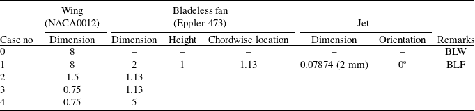
A comprehensive 2D analysis was carried out to characterise the geometric parameters associated with the integration process of semi-annular bladeless fans, which includes height from the baseline wing surface (analogous to fan’s radius in a 3D scenario), chordwise location and orientation of the fan. Four geometric configurations were analysed as per geometric parameters presented in Table 1. For a baseline wing configuration (BLW), a chord length of 8 inches was selected. For bladeless fan configurations, the geometric variation includes the fan’s height from the chord of the baseline wing and chordwise location over the baseline wing (Fig. 3). The orientation of fan was set to 0o for all the configurations as per the preferred setting highlighted in Ref. (Reference Mehmood, Shahzad, Qadri, Salamat, Shams and Masud13). The configuration with a fan’s height of 1 inch and chordwise location of 1.13 inches from the leading edge of the baseline wing is declared as baseline fan configuration (BLF). The flow on the baseline wing separates from the leading edge as the AoA is increased. Therefore, the selection of the chordwise location of 1.13 inches for the leading-edge configurations will put the maximum thickness of the bladeless fan aerofoil and baseline wing aerofoil at the same location i.e. the minimum gap between the two aerofoil surfaces. This arrangement will ensure lower static pressure and higher flow velocity. For trailing-edge configurations, the bladeless fan was placed 5 inches from the leading edge of the baseline wing. This arrangement will ensure that the bladeless fan is sufficiently ahead of the trailing edge of the baseline wing and would be effective in maintaining positive flow on the wing.
Geometric configuration of test cases

Note: All dimensions are in inches.
Geometric configuration of test cases (a) variation for leading-edge configurations; (b) variations for trailing-edge configurations.

Figure 3 Long description
The diagram illustrates two geometric configurations of test cases. In part (a), the leading-edge configurations vary with a distance labeled as x equals 1.13 and heights labeled as h equals 0.75, 1, and 1.5. In part (b), the trailing-edge configurations vary with a distance labeled as x equals 5 and a height labeled as h equals 0.75. Each part shows a cross-sectional view of an aerodynamic shape with arrows indicating measurements and variations.
The geometry was created in the ANSYS Design Modeler with Eppler-473 selected as an aerofoil cross-section for the bladeless fan and NACA0012 for the baseline wing. The bladeless fan and wing geometries were enclosed in a rectangular cross-section acting as a fluid domain. Eppler-473 (stall angle 15∼17°) is the preferred aerofoil for bladeless application [Reference Guoqi, Peifeng, Baoling, Yingzi, Yongjun and Zhe36–Reference Jafari, Afshin, Farhanieh and Sojoudi39], whereas symmetric aerofoil NACA0012 (stall angle 12∼15°) was selected for the wing due to the online availability of performance data set for ease of comparison and to check the fidelity of bladeless fan on the wing at 0° AoA. Generally, the stall angle for the bladeless fanjet should be higher as compared to the wing to ensure the flow on the bladeless fanjet surface is attached and operational at the stalling angle of the baseline wing. If the bladeless fanjet stalls earlier than the wing, it will introduce flow instabilities leading to an early stall of the baseline wing as well.
2.1 Solver setting and boundary conditions
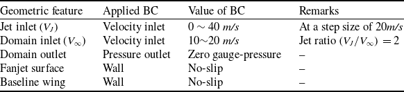
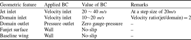
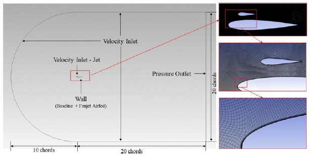
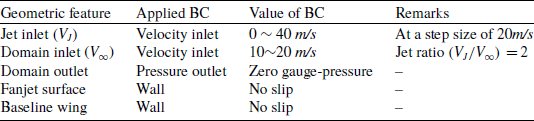
The Fluent module of ANSYS is used for 2D, transient, incompressible viscous analysis of the flow field around the configurations under study. A pressure-based solver was used with SST-kw selected as a turbulence model. The jet width acts as an inlet for the entire domain, whereas the domain boundary acts as a wind inlet and outlet according to the requirement. Both the inlets were modelled as velocity inlets to simulate jet flow and the incoming free stream. The outlet was modelled as a pressure outlet with zero-gauge pressure, and the aerofoils surfaces as no-slip walls. All the cases were simulated for various wind and jet velocities to capture the true effect of geometric variation. The domain and boundary conditions are annotated in Fig. 4 and Table 2. The selected domain inlet velocities of 10 and 20 m/s and wing chords of 8 inches correspond to Reynolds number (Re) of 1.37 × 10⁵ and 2.72 × 10⁵, respectively. A velocity ratio (bladeless fanjet velocity/freestream velocity) was kept as 2 for the present computational work owing to experimental capability limitation. Generally, the jet ratio
 $\left( {{V_J}/{V_\infty }} \right)\;$
must be greater than the ratio of local velocity at the maximum thickness of baseline wing to free stream
 $\left( {{V_{0.25c}}/{V_\infty }} \right)$
to ensure inducement and entrainment of the surrounding flow in the presence of free stream conditions.
Boundary conditions (BC) for the computational setup

Table 2 Long description
The table outlines boundary conditions for a computational setup, focusing on geometric features, applied boundary conditions, values of those conditions, and remarks. The first column lists geometric features such as jet inlet, domain inlet, domain outlet, fanjet surface, and baseline wing. The second column specifies the type of boundary condition applied, including velocity inlet, pressure outlet, and wall. The third column provides the values of these boundary conditions, ranging from 0 to 40 meters per second for velocity inlets and zero gauge pressure for the pressure outlet. The fourth column offers remarks, such as the step size for the jet inlet and the jet ratio for the domain inlet. Notable trends include the use of velocity inlets for both jet and domain inlets and the consistent application of no-slip conditions for walls.
Note: A jet ratio of 2 is higher than the local velocity ratio
 $\left( {{V_{0.25c}}/{V_\infty }} \right)$
for the computational cases.
Computational domain, boundary conditions and domain meshing. Fanjet and bladeless fan have been used interchangeably in this work.

Figure 4 Long description
The diagram illustrates a computational domain for a bladeless fan. It features a velocity inlet at the top, a velocity inlet for the jet in the middle, and a pressure outlet on the right side. The wall, labeled as the baseline plus fanjet airfoil, is depicted with a curved shape. The diagram includes detailed views of the fanjet and the surrounding mesh structure. Arrows indicate the direction of airflow, and the overall structure shows the interaction between the jet and the surrounding air, demonstrating the principles of inducement and entrainment.
Mesh independence study. The selection parameters are C l and C d at Re of 2.74× 10⁵. A mesh size of 0.987 m was selected with a % difference of 1.6 and 1.65% for C l and Cd, respectively.

Figure 5 Long description
A line graph showing mesh independence study with C l and C d at Re of 2.74 105. The x axis represents mesh size in millions ranging from 0.4 to 1.2. The left y axis represents C l values ranging from 0.52 to 0.68. The right y axis represents C d values ranging from 0.012 to 0.018. The black line with square markers represents C l values at 5 degrees angle of attack, while the blue line with square markers represents C d values at 5 degrees angle of attack. The selected mesh size is 0.987 million, marked with red boxes on both lines. All values are approximated.
2.2 Mesh independence
A mesh independence study was conducted using drag and lift as a reference parameter. Only free-stream wind was simulated with no input from the bladeless fanjet. Meshing was done using the ANSYS Mesh module, and cases were simulated in the ANSYS Fluent module. Based on the drag and lift values computed from the test cases, a mesh size of 0.978 m was selected for further analysis. The domain mesh is presented in Fig. 4 and mesh independence study in Fig. 5.
2.3 Validation
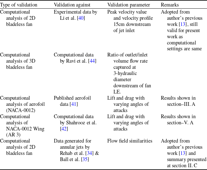
Considering the complexity of the problem and non-availability of scientific investigations for this specific integrated domain, the authors exercised careful judgement and due diligence in selecting an appropriate validation strategy. Multiple cases with varying configurations were employed for validation, including bladeless fan and selected baseline aerofoil experimental and computational studies reported by various researchers. The summary of the validation process is presented in Table 3.
Summary of the validation work carried out for 2D and 3D cases

Table 3 Long description
The table presents a summary of the validation work conducted for 2D and 3D cases. It consists of four columns: Type of validation, Validation against, Validation parameter, and Remarks. The table has six rows, each detailing different validation scenarios. Row 1: Computational analysis of 2D bladeless fan, Experimental data by Li et al., Peak velocity value and velocity profile 15 centimeters downstream of jet inlet, Adopted from author's previous work, still valid for present work as computational settings are same. Row 2: Computational analysis of 3D bladeless fan, Computational data by Ravi et al., Ratio of outlet/inlet volume flow rate captured at 3-hydraulic diameter downstream of fan LE. Row 3: Computational analysis of aerofoil (NACA-0012), Published aerofoil data, Lift and drag with varying angles of attacks, Results shown in section III. A. Row 4: Computational analysis of NACA-0012 Wing (AR 3), Computational data by Shahrooz et al., Lift and drag with varying angles of attacks, Results shown in section V. A. Row 5: Computational analysis of 2D bladeless fan, Data generated for annular jets by Rehab et al. and Ball et al., Flow field similarities, Adopted from author's previous work and summary presented at section II. C.
Validation study for 2D cases. Velocity profile downstream of bladeless fan was captured and compared against the experimental data captured by Li et al. [Reference Li, Deng and Lai40].

Figure 6 Long description
The image contains multiple graphs and diagrams related to a validation study for 2D cases. The top left section shows two shapes with annotations indicating validation against experimental data from Li et al. and published airfoil data for NACA 0012. The top right section features a line graph comparing the coefficient of lift and drag against the angle of attack for both bladeless fan (BW) and airfoil data. The bottom left section displays a diagram of the computational domain with dimensions and boundary conditions for the bladeless fan. The bottom right section presents a line graph comparing vertical distance against velocity, with data from present computational fluid dynamics (CFD) work and experimental data.
As the present work is the continuation of the author’s previous work [Reference Mehmood, Shahzad, Qadri, Salamat, Shams and Masud13] with the same 2D computational setup to analyse bladeless fan over baseline wing, therefore the validation process adopted for the bladeless fan holds good for present study as well. An overview of the validation is presented here for reference. The validation was carried out against the experimental work conducted by Li et al. [Reference Li, Deng and Lai40]. Based on the geometric parameters of Li et al. [Reference Li, Deng and Lai40], a 2D axis-symmetry case was modelled and meshed in an ANSYS environment. The simulations were conducted using a pressure-based solver with SST-kw as the turbulence model. As per the experimental setup [Reference Li, Deng and Lai40], the velocity profile at 15 cm downstream of the jet inlet from the validation work was compared with the experimental results. The velocity profile was successfully captured with peak velocity differing by a maximum of 3.9%, thus successful validation for the computational setup was achieved (Fig. 6). For further details on validation studies, readers are referred to authors’ previous study [Reference Mehmood, Shahzad, Qadri, Salamat, Shams and Masud13].
Lift and drag coefficients of baseline wing (a) comparison with published aerofoil data [41]; (b) comparison at different Re (BLW-1 and BLW-2).

Figure 7 Long description
The line graph consists of two subplots labeled (a) and (b). Subplot (a) compares the lift and drag coefficients of a baseline wing with published airfoil data. The x-axis represents the angle of attack in degrees, ranging from negative 2 to 16 degrees. The y-axis on the left represents the coefficient of lift, ranging from 0 to 1.2, and the y-axis on the right represents the coefficient of drag, ranging from 0 to 0.6. The data series include BWL coefficient of lift, airfoil coefficient of lift, BWL coefficient of drag, and airfoil coefficient of drag. Subplot (b) compares the lift and drag coefficients at different Reynolds numbers, labeled as Re 2 and Re 1. The x-axis represents the angle of attack in degrees, ranging from negative 2 to 16 degrees. The y-axis on the left represents the coefficient of lift, ranging from 0 to 1.2, and the y-axis on the right represents the coefficient of drag, ranging from 0 to 0.6. The data series include coefficient of lift at Re 2, coefficient of lift at Re 1, coefficient of drag at Re 2, and coefficient of drag at Re 1. All values are approximated.
3.0 Analysis of 2D configurations
3.1 Baseline wing configuration
The baseline wing was analysed to set the reference for bladeless fan configurations. The test case was simulated at Re of 2.74 × 10⁵ and 1.37 × 10⁵ for a range of AoA until the stall angle to determine lift and drag coefficients. As per Fig. 7, the stall angle and maximum lift coefficient are consistent with the aerofoil data. Similarly, the drag profile is also consistent with the aerofoil data set, thus further validating the authenticity of the simulations. As the Re decreased, the overall lift decreased and drag increased; again, the trends are consistent with the established theoretical trends. The BLW-1 and BLW-2 correspond to Re1 (1.37 × 10⁵) and Re2 (2.74 × 10⁵), respectively. Pressure plots were presented at 0°, 5° and 10° to support the variation in lift and drag (Fig. 8).
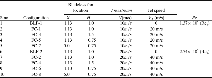
Bladeless fan/fanjet configurations (FC), its dimensional parameters, and operating conditions

Table 4 Long description
The table presents a comparison of bladeless fan configurations, their dimensional parameters, and operating conditions. It consists of ten rows and six columns. The columns are labeled as S no, Configuration, Bladeless fan location, Freestream, Jet speed, and Re. The Bladeless fan location is further divided into X and H. The Freestream column lists the velocity in meters per second, and the Jet speed column lists the velocity in meters per second. The Re column lists the Reynolds number. The table includes configurations such as BLF-1, FC-1, FC-3, FC-5, FC-7, BLF-2, FC-2, FC-4, FC-6, and FC-8, with varying dimensions and operating conditions.
Different bladeless fan configurations were tested under the same solver settings with different jet speeds. The geometric details of the configurations tested are presented in Table 4. The cases for Re1 are represented by odd number configurations and Re2 with even numbers.
Pressure plots at various angles of attack (a) 0°, (b) 5° (c) 10°. There is no variation of ΔP (difference in pressure of lower and upper surface of the aerofoil) at 0°; thus the lift is zero for both configurations. As the angle is increased, the ΔP increases more for Re2 as compared to Re1; therefore, more lift for BLW-2 as compared to BLW-1.

Figure 8 Long description
The line graph displays pressure plots at various angles of attack: (a) 0 degrees, (b) 5 degrees, and (c) 10 degrees. The x-axis represents the chord length in meters, ranging from 0 to 0.20 meters. The y-axis represents the pressure in Pascals, with different scales for each subplot: (a) ranging from -150 to 250 Pascals, (b) ranging from -500 to 300 Pascals, and (c) ranging from -1200 to 400 Pascals. Two data series are plotted: BLW-1 represented by black squares and BLW-2 represented by red triangles. At 0 degrees angle of attack, there is no variation in pressure difference between the lower and upper surfaces of the aerofoil, resulting in zero lift for both configurations. As the angle of attack increases to 5 and 10 degrees, the pressure difference increases more for BLW-2 compared to BLW-1, indicating more lift for BLW-2. All values are approximated.
3.2 Baseline fan configurations
The BLF, i.e. V J = 0 m/s, are compared with the corresponding BLW and results are presented in Figs 9 and 10. The variation in the results is purely based on the geometry of the bladeless fanjet and its interaction with the wing itself as no blowing is carried out in the baseline thruster cases. It can be observed that at Re1, the BLW1 is superior in performance to the BLF1 configuration, however, as the Re is increased (Re2), the BLF2 becomes slightly better than the BLW2, especially in the post-stall region. The pressure plots captured for BLW1 and BLF1 at a 10° angle are presented in Fig. 11 for correlation with the trends.
Comparison of BLW1 and BLF1 at Re1 – (a) C l (b) C d .

Figure 9 Long description
The line graph consists of two subplots labeled (a) and (b). Subplot (a) shows the lift coefficient (C l) versus the angle of attack (AoA) in degrees for BLW1 and BLF1. BLW1 is represented by black squares, and BLF1 is represented by blue circles. The lift coefficient increases with the angle of attack, peaking around 10 degrees for both designs, then slightly decreases. Subplot (b) shows the drag coefficient (C d) versus the angle of attack (AoA) in degrees for BLW1 and BLF1. The drag coefficient remains relatively low and constant up to around 10 degrees, after which it increases sharply for both designs. All values are approximated.
At Re1 (1.37 × 10⁵), a negligible difference was observed in the lift values till 5° AoA; however, beyond 5° the BLF1 showed degradation in the lift values till stalling AoA. The lift for the BLF1 configuration is the sum of the lift produced by the wing and bladeless fan. From the pressure profile captured at 10°, it can be observed that the bladeless fan itself is generating negative lift due to low-pressure values at the pressure side of the aerofoil, thus making the overall lift much less as compared to BLW1. In the post-stall region, the BLF1 maintained its lift whereas the lift for BLW1 drastically reduced confirming the complete stall of the baseline wing. The streamline plots are captured in the post-stall region to establish the flow physics (Fig. 12). A strong formation and shedding of the vortex can be seen on BLW1, which degrades the overall lift generation capability of the wing, whereas a steady vortex system is formed on BLF1. The air flowing through the channel path between the wing and bladeless fanjet (BLF1) under a favourable pressure gradient suppresses the flow detachment from the leading edge of the baseline wing as observed in BLW1 and thus retains sufficient lift. The drag values for BLF1 are higher as compared to BLW1 in the pre-stall region and showed improvement over BLW1 in the post-stall region because of lesser pressure drag as compared to BLW1.
Comparison of BLW2 and BLF2 at Re2 – (a) C l (b) C d .

Figure 10 Long description
The image contains two line graphs side by side. The left graph (a) shows the lift coefficient (C l) versus the angle of attack (AoA) in degrees for BLW2 and BLF2. The right graph (b) shows the drag coefficient (C d) versus the angle of attack (AoA) in degrees for BLW2 and BLF2. Both graphs have data points marked with black squares for BLW2 and red circles for BLF2. In graph (a), the lift coefficient increases with the angle of attack, peaking around 10 degrees before decreasing. In graph (b), the drag coefficient remains relatively low and stable up to about 10 degrees, after which it increases sharply. The comparison indicates how the lift and drag coefficients vary with the angle of attack for the two different configurations.
Pressure plots for BLW1 and BLF1 configurations at 10o AoA. A clear pressure variation can be observed for the BLF1 configuration which degrades the lift as compared to the BLW1 configuration.

Figure 11 Long description
A heat map showing pressure variations for BLW1 and BLF1 configurations at 10 degrees angle of attack. The heat map consists of two panels, each representing a different configuration. The left panel shows the BLW1 configuration, while the right panel shows the BLF1 configuration. The color scale at the bottom ranges from -300 to 200, with blue indicating lower pressure and red indicating higher pressure. The BLF1 configuration exhibits a clear pressure variation, which degrades the lift compared to the BLW1 configuration. The heat map highlights regions of high and low pressure, with notable differences between the two configurations.
At Re2 (2.74 × 10⁵), BLF2 is generating more lift as compared to BLW2. The difference is negligible in the pre-stall region (Fig. 13) and more pronounced in the post-stall region (Fig. 14). The drag showed similar behaviour, in the pre-stall region i.e. the values for BLF2 are higher than BLW2; however, noticeable improvement was observed in the post-stall region. In the post-stall region, strong vortex formation and shedding were observed on BLW2, whereas a stable vortex formation was observed on BLF2 (Fig. 14).
Streamline plots at 15° AoA (post-stall region) for (a) BLF1 and (b) BLW1.

Figure 12 Long description
A heat map showing streamline plots at 15 degrees angle of attack in the post-stall region for two different bladeless fan designs, BLF1 and BLW1. The heat map consists of two subplots labeled (a) and (b). Subplot (a) represents the streamline plot for BLF1, while subplot (b) represents the streamline plot for BLW1. The color scale at the bottom ranges from -500 to 200, with blue indicating lower values and red indicating higher values. The streamline plots show the flow patterns around the bladeless fan designs, with distinct vortices and flow separations visible. The plots highlight the differences in flow characteristics between the two designs in the post-stall region.
Pressure profile of BLW2 and BLF2 (wing only) at 5° AoA.

Figure 13 Long description
A line graph compares the pressure profiles of BLW2 and BLF2 at a 5-degree angle of attack. The x-axis represents the chord location in meters, ranging from 0 to 0.20 meters. The y-axis represents the pressure in Pascals, ranging from -800 to 400 Pascals. The graph includes two data lines: one for BLW2 represented by blue diamonds and another for BLF2-Wing represented by red triangles. The location where the fanjet modifies the pressure profile on the wing is indicated with an arrow. All values are approximated.
Pressure and streamline plots for BLW2 (top) and BLF2 (bottom) configurations at 15° AoA (post-stall region). The variation in aerodynamic forces (see Fig. 9) for both the cases is attributted to the difference in the vortex system formation and associated pressure profile.

Figure 14 Long description
A heat map displays pressure and streamline plots for two different configurations, labeled as BLW2 and BLF2, at a high angle of attack in the post-stall region. The heat map uses a color scale ranging from deep blue to dark red, indicating varying pressure values. The top section shows the BLW2 configuration, while the bottom section shows the BLF2 configuration. The color intensity represents the pressure distribution, with blue indicating lower pressure and red indicating higher pressure. Streamlines are overlaid to show the flow patterns around the configurations. Notable regions include areas of high and low pressure, as well as the formation of vortices. The overall trend shows significant differences in the vortex systems and associated pressure profiles between the two configurations, which contribute to variations in aerodynamic forces.
Comparison of bladeless fanjet configurations with baseline wing at low Re (10 m/s freestream velocity) (a) lift coefficient; (b) drag coefficient.

Figure 15 Long description
The line graph compares bladeless fanjet configurations with a baseline wing at a low Reynolds number, specifically at a freestream velocity of 10 meters per second. The graph consists of two subplots: (a) lift coefficient and (b) drag coefficient, both plotted against the angle of attack (AoA) in degrees. In subplot (a), the lift coefficient (C_l) is plotted on the y-axis, ranging from 0 to 1, while the angle of attack (AoA) is plotted on the x-axis, ranging from 0 to 20 degrees. The data series include BLW1, FC1, FC3, FC5, and FC7, each represented by different symbols and line styles. In subplot (b), the drag coefficient (C_d) is plotted on the y-axis, ranging from 0 to 0.3, while the angle of attack (AoA) is plotted on the x-axis, ranging from 0 to 20 degrees. The same data series are represented here as well. The lift coefficient generally increases with the angle of attack up to a certain point, after which it starts to decrease. The drag coefficient increases with the angle of attack, with notable spikes at higher angles. All values are approximated.
3.3 Bladeless fanjet configurations
Different fan configurations were simulated as mentioned in Table 4 and the results were compared with corresponding BLW configurations. The lift and drag for all the configurations were calculated and presented in Figs 15 and 20.
-
1. Low Free Stream Condition (Re 1 = 1.37 × 10 5 ). In the pre-stall region, negligible variation was observed at 0° AoA for all cases. At 5° AoA, fan configuration FC5 and FC7 performance was lower, whereas FC1 and FC3 were at par with the BLW1. At 10° AoA, except FC3, all the fan configurations have low C l values as compared to BLW1 (Fig. 15a). In the pre-stall region, all the bladeless fan configurations have higher drag coefficients as compared to BLW1. Detailed flow analysis was carried out to ascertain the reason for the underperformance of various bladeless fan configurations. Figure 16 compares the pressure distributions of FC3 and BLW1 at 5° and 10° AoA. The pressure distribution of FC3 is negligibly disturbed by the presence of active fan blowing at 20 m/s. Thus, FC3 has a comparable lift value with BLW1. Pressure distributions for FC5 and FC7 are presented in Fig. 17. The fan effectively modifies the pressure distribution in both cases. Strong suction is created in the case of FC5 due to lesser channel height. However, the stagnation pressure created at the leading edge of the bladeless fanjet also modifies the pressure distribution on the leading edge of the wing as can be observed in Fig. 18. The change in pressure (ΔP) for FC5 is smaller than the BLW1, coupled with the small lift produced by the fan, the overall lift of FC5 is lower than BLW1. At 10° AoA, the trend is similar for pressure distribution, ΔP is lower as compared to BLW1 and FC7, thus having lower lift among the configurations.
Pressure distribution on the upper and lower surface of BLW1 and FC3 (wing only) at (a) 5° AoA; (b) 10° AoA.

Figure 16 Long description
Two line graphs compare the pressure distribution on the upper and lower surfaces of BLW1 and FC3 at two different angles of attack. The x-axis represents the chord location in meters, ranging from 0 to 0.2 meters. The y-axis represents the pressure in Pascals, ranging from -150 to 100 Pascals in graph (a) and from -300 to 100 Pascals in graph (b). The red line with diamond markers represents the FC3-Wing, while the blue line with square markers represents BLW1. In graph (a), at a 5-degree angle of attack, the pressure distribution shows a peak and trough pattern for both surfaces, with the FC3-Wing exhibiting slightly different pressure values compared to BLW1. In graph (b), at a 10-degree angle of attack, the pressure distribution follows a similar pattern but with more pronounced peaks and troughs, indicating higher pressure variations. All values are approximated.
Pressure distribution on the upper and lower surface of BLW1 and (a) FC5 (wing only) at 5° AoA; (b) FC7 (wing only) at 5° AoA; (c) FC5 and FC7 (wing only) at 10° AoA.

Figure 17 Long description
The line graph presents the pressure distribution on the upper and lower surfaces of BLW1 and FC5 Wing at a 5-degree angle of attack. The x-axis represents the chord location in meters, ranging from 0 to 0.2 meters. The y-axis represents the pressure in Pascals, ranging from -150 to 100 Pascals. The graph includes two data lines: one for BLW1 represented by blue circles and a solid blue line, and another for FC5 Wing represented by red triangles and a solid red line. The pressure distribution shows significant variations, with notable peaks and troughs indicating areas of high and low pressure along the chord location. All values are approximated.
Bladeless fan also modifies the pressure distribution on FC7; however, the net ΔP for FC7 is lower than BLW1 and hence lower lift values. At 10° AoA, the flow toward the trailing edge of the wing is detached from the surface of the wing. The fan located at the trailing edge of the wing becomes ineffective in creating lower pressures, thus the overall effect is much closer to BLW1. In the post-stall region, the lift for all the bladeless fan configurations is higher as compared to the baseline wing. The baseline wing stalls at 12° AoA with a separated flow on most parts of the wing, but in cases of bladeless fan configurations, the flow is attached thus having a higher lift.
Drag for all the configurations in the pre-stall regions are higher than the baseline wing configuration. FC7 has the lowest drag among all the fan configurations mainly due to the similar pressure distribution as on the baseline wing. In the post-stall region, the drag values are lower for all configurations except FC7. The main reason behind lower drag is low-pressure drag due to the attached flow. A vortex shedding phenomenon was observed on the FC7, which resulted in high drag values (Fig. 19). The flow detached from the leading edge of the main wing and was further aggravated by the fan located near the trailing edge. Sinusoidal behaviour was observed in FC7 where flow kept on attaching and detaching with overall higher drag values.
-
2. High Free Stream Conditions (Re 2 = 2.74 × 10 5 ). In the pre-stall region, negligible variation was observed at 0° to 5° AoA for all cases except FC8, which has lower lift values as compared to all other configurations including baseline BLW2 (Fig. 20). The pressure profiles for FC8 and BLW2 are presented in Fig. 21. It can be observed that ΔP is lower for the FC8 as compared to BLW2, but the negative lift created by the bladeless fanjet further reduces the overall lift for the FC8. At 10o AoA, FC8 and FC6 have lower lift values and FC4 and FC2 have higher lift values as compared to BLW2. FC4 and FC6 pressure profiles are presented in Fig. 22. The ΔP for FC4 is better as compared to FC6 and comparable to BLW2. The overall pressure profile of FC4 with bladeless fanjet is better than BLW2 and that of FC6 is less than BLW2. In the post-stall region, the lift for all the bladeless fanjet configurations is higher as compared to the baseline wing with a maximum increase of 71%. The baseline wing stalls at 12° AoA with separated flow on most parts of the wing, but in cases of bladeless fanjet configurations, the flow is attached thus having a higher lift. A 15° stall angle (25% increment) was observed for fanjet configurations.
Pressure distribution for FC7 (top), BLW1 (middle) and FC5 (bottom) configurations at 10° AoA. The pressure variation on the baseline wing in the presence of fan can be observed.

Figure 18 Long description
A heat map displays the pressure distribution for three different configurations at a 10-degree angle of attack. The top section shows the pressure distribution for the FC7 configuration, the middle section for the BLW1 configuration, and the bottom section for the FC5 configuration. The color scale ranges from blue, indicating lower pressure, to red, indicating higher pressure. The heat map reveals variations in pressure across the wing surfaces, with notable differences between the configurations. The baseline wing's pressure variation in the presence of a fan is observable, highlighting areas of high and low pressure.
In the pre-stall region, drag values for all the configurations are higher than the BLW2 configuration (a minimum of 50% increment in zero-lift drag), however, in the post-stall region, values are lower than the baseline wing for all configurations mainly due to lesser pressure drag. A minimum of 39% reduction in drag at 15° AoA was observed.
3.4 Selection of bladeless fanjet configuration for 3D experimental and computational analysis
-
1. Aerodynamic Efficiency. The drag polar and C l /C d versus α (AOA) were plotted in Fig. 23 for all configurations. Based on the results, it was inferred that installation of a bladeless fanjet toward the trailing edge was not a viable option as post-stall drag increment was more for this configuration at low Re. For leading-edge configurations, FC3 provided better lift-to-drag (L/D) values at low Reand post-stall characteristics. At high Re, FC2 and FC4 have achieved higher efficiency than the rest of the configurations.
-
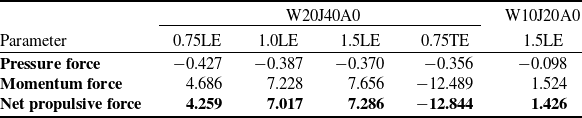
2. Net Propulsive Force. As the bladeless fanjet is also going to produce thrust for the respective configurations, it was imperative to calculate the net propulsive force for the configurations. Although propulsion analysis was not part of the research scope, to select a feasible configuration, a sample net propulsive force analysis was carried out. In case the net propulsive force came out to be negative, the respective configuration under operating conditions would not be sustainable. The net propulsive force is defined as the thrust force minus the drag force of the configuration. To calculate, the net propulsive force in the forward direction i.e. along the x-axis, a control volume was drawn over the configuration, as shown in Fig. 24. The pressure is acting perpendicular to the control boundaries; therefore, the top and bottom pressure profiles were not included in the calculation as they will only contribute toward normal force. Momentum flux was considered for all the faces along the x-axis. Net propulsive force is then the summation of net momentum flux and pressure forces along the x-axis. For reference calculation, only cases with zero AoA were selected for comparison. The values for different configurations are presented in Table 5.
-
3. Selection of Configuration. From the values, it can be observed that as the bladeless fanjet height increases at the leading edge, the net propulsive force increases due to increase in momentum flux at the rear. The trailing edge configuration failed to generate thrust, as the outlet momentum flux is less as compared to the inlet, mainly because of very little entrainment close to the wing configuration. Higher jet speed (V J = 40 m/s) produces higher propulsive force and is preferred. Based on aerodynamics (Fig. 23) and propulsive analysis (Table 5), FC2 and FC4 have shown better results as compared to the rest of the configurations. Keeping in view the wingspan limitation for wind tunnel tests, FC2 (smaller radius as compared to FC4) was selected as a baseline geometry for further 3D computational and experimental analysis.
Pressure and streamline plots for – FC7 (left) and BLW1 (right). A strong vortex formation can be seen in both cases. The bladeless fan located near the trailing edge further aggravates the detached flow, thus increasing the overall drag for the FC7.

Figure 19 Long description
A heat map showing pressure and streamline plots for FC7 and BLW1 with strong vortex formations. The left plot represents FC7, and the right plot represents BLW1. Both plots display a color scale ranging from -500 to 200 pascals, indicating static pressure. The streamlines show the flow of air around an object, with noticeable vortex formations in both cases. The bladeless fan located near the trailing edge in the FC7 plot aggravates the detached flow, increasing overall drag. The color intensity varies, with darker regions indicating lower pressure and lighter regions indicating higher pressure. The plots highlight the differences in flow characteristics and pressure distribution between the two configurations.
Comparison of bladeless fanjet configurations with baseline wing at high reynolds (20 m/s freestream velocity); (a) lift coefficient; (b) drag coefficient.

Figure 20 Long description
The line graph consists of two subplots labeled (a) and (b). Subplot (a) shows the lift coefficient (C l) versus angle of attack (AoA) in degrees for five different configurations: FC-6, FC-4, FC-8, FC-2, and BLW2. Subplot (b) shows the drag coefficient (C d) versus angle of attack (AoA) in degrees for the same configurations. Each configuration is represented by a different colored line and marker: FC-6 with black squares, FC-4 with red circles, FC-8 with green triangles, FC-2 with blue inverted triangles, and BLW2 with gray diamonds. The lift coefficient increases with the angle of attack up to around 10 degrees and then decreases. The drag coefficient generally increases with the angle of attack. All values are approximated.
4.0 Computational methodology for 3D analysis
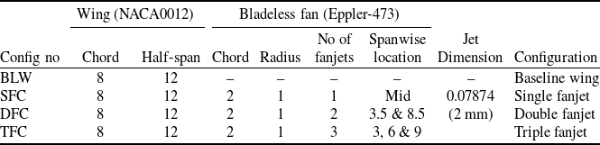
The selected 2D configuration was translated into 3D model and a comprehensive 3D analysis was carried out to characterise the geometric parameters associated with the integration process of semi-annular bladeless fan with the baseline wing surface. The parameters include the number of fan units, orientation and their spanwise location. Four geometric configurations were analysed as per geometric parameters presented in Table 6. The geometric variation includes the number of bladeless fanjets and spanwise location over the wing (Fig. 25). The baseline wing with a chord 8-inch and half span 12-inch was modeled in ANSYS Design Modeler with NACA0012 as a cross-sectional aerofoil. The bladeless fan was created with a cross-sectional aerofoil Eppler-473. A semi-annular fan with a 2-inch chord and a radius of 1 inch was attached to the upper surface of the wing. The baseline wing with an aspect ratio (AR) of 3 has a stalling angle of ∼30° [Reference Shahrooz and Abdulkareem42] against the stalling angle of ∼12° for the aerofoil section [Reference Chen, Li and Nguyen43].
Net propulsive force for various bladeless fanjet configurations

Table 5 Long description
The table presents a comparison of net propulsive force for various bladeless fanjet configurations. It includes data for pressure force, momentum force, and net propulsive force across different parameters and configurations. The table has 5 rows and 8 columns, with headers for Parameter, Pressure force, Momentum force, and Net propulsive force. The configurations compared are W20J40A0 and W10J20A0, with specific values for 0.75LE, 1.0LE, 1.5LE, 0.75TE, and 1.5LE. Notable trends include higher net propulsive force for configurations with higher bladeless fanjet height at the leading edge, indicating better performance. The trailing edge configuration shows negative net propulsive force, indicating it failed to generate thrust. The data highlights the importance of momentum flux and pressure forces in determining the net propulsive force.
Note: In nomenclature W20J40A0, W stands for free stream speed, J for jet speed and A for jet orientation, and numeric values represent the associated operational condition of these parameters.
Comparison of FC8 with BLW-2 at 5° AoA (a) BLW2 and FC8 (wing only); (b) FC8 fanjet.

Figure 21 Long description
The image contains two line graphs. The first graph (a) compares static pressure against chord location for BLW2-Wing and FC8-Wing configurations. The BLW2-Wing data is represented by black squares, and the FC8-Wing data is represented by red circles. The second graph (b) shows static pressure against chord location for the FC8-Fanjet configuration, represented by red triangles. The x-axis represents chord location in meters, and the y-axis represents static pressure in Pascals. The BLW2-Wing and FC8-Wing graph shows data points ranging from 0 to 0.2 meters on the x-axis and from -500 to 300 Pascals on the y-axis. The FC8-Fanjet graph shows data points ranging from 0.12 to 0.18 meters on the x-axis and from -500 to 300 Pascals on the y-axis. All values are approximated.
FC4 and FC6 comparison with BLW-2 at 10° AoA: (a) wing only; (b) FC4 and fC6 fanjets.

Figure 22 Long description
The line graph presents a comparison of static pressure across chord location for different wing configurations and fanjet settings. The x-axis represents the chord location in meters, ranging from 0 to 0.20 meters in graph (a) and from 0.02 to 0.08 meters in graph (b). The y-axis represents the static pressure in Pascals, ranging from -1200 to 400 Pascals in graph (a) and from -1000 to 200 Pascals in graph (b). Graph (a) includes data lines for BLW2-Wing, FC4-Wing, and FC6-Wing, each showing distinct pressure profiles. Graph (b) includes data lines for FC4-Fanjet-upper, FC4-Fanjet-lower, FC6-Fanjet-upper, and FC6-Fanjet-lower, each displaying unique pressure variations. The data lines show how static pressure changes along the chord location for each configuration, highlighting differences in aerodynamic performance. All values are approximated.
Drag polar and C l /C d versus α plots: (a) C l /C d versus α @ Re1; (b) drag polar; @ Re1; (c) C l /C d versus α @ Re2; (d) drag polar @ Re2.

Figure 23 Long description
The image contains four graphs analyzing the aerodynamic performance of various flow control devices. The first graph (a) plots the lift-to-drag ratio (C l /C d) against the angle of attack (AoA) for different devices at Reynolds number 1 (Re1). The second graph (b) shows a drag polar plot of lift coefficient (C l) versus drag coefficient (C d) at Re1. The third graph (c) plots the lift-to-drag ratio (C l /C d) against the angle of attack (AoA) for different devices at Reynolds number 2 (Re2). The fourth graph (d) shows a drag polar plot of lift coefficient (C l) versus drag coefficient (C d) at Re2. Each graph includes multiple data series represented by different symbols and colors, indicating the performance of various flow control devices. The graphs illustrate how different devices affect aerodynamic efficiency and stall delay under varying conditions.
The Fluent module of ANSYS is used to capture 3D, transient, incompressible viscous analysis of the flow field created by the present geometry. A pressure-based solver was used with SST-kw selected as a turbulence model for capturing turbulence in the flow field. The domain and boundary conditions are annotated in Fig. 26 and Table 7. Mesh of 7.93 m was selected based on mesh independence study with a y + around 1.1∼3.2. All the cases were simulated for various wind and jet velocities to capture the true effect of geometric variation.
Geometric configuration of 3D test cases

Table 6 Long description
The table presents a comparison of geometric configurations for 3D test cases involving the integration of bladeless fans with a baseline wing. It includes four configurations labeled BLW, SFC, DFC, and TFC. Each configuration details the chord and half-span of the wing, the chord and radius of the bladeless fan, the number of fanjets, their spanwise location, jet dimension, and configuration type. The baseline wing has a chord of 8 inches and a half-span of 12 inches. The bladeless fan has a chord of 2 inches and a radius of 1 inch. The configurations vary in the number of fanjets (single, double, and triple) and their spanwise locations. The jet dimension for the single fanjet configuration is 0.07874 inches (2 millimeters). The table provides a comprehensive overview of the geometric parameters associated with the integration process.
Note: All dimensions are in inches.
Control volume for net propulsive force calculation.

Figure 24 Long description
The diagram illustrates a control volume used for calculating net propulsive force. It features a rectangular boundary with arrows indicating the flow of mass and pressure forces. The top and bottom arrows represent the mass flow velocities at the top and bottom, while the left and right arrows denote the mass flow velocities at the front and rear. Additionally, there are arrows indicating the pressure forces at the front and rear of the control volume.
Geometric configuration of 3D test cases.

Figure 25 Long description
The diagram illustrates three distinct geometric configurations of 3D test cases for flow control devices on a wing surface. Configuration 1 features a single vortex generator positioned centrally on the wing. Configuration 2 displays two vortex generators, one near the leading edge and another further back. Configuration 3 shows three vortex generators spaced along the wing. Each configuration includes detailed measurements: Configuration 1 has a 1-inch height and 2-inch width vortex generator placed 6 inches from the leading edge. Configuration 2 has two vortex generators, each with a 1-inch height and 2-inch width, positioned 8.5 inches and 3.5 inches from the leading edge, respectively. Configuration 3 features three vortex generators, each with a 1-inch height and 2-inch width, spaced 9 inches and 6 inches apart, with the first generator 3 inches from the leading edge.
Boundary conditions (BC) applied to various geometric features

Table 7 Long description
The table presents boundary conditions applied to various geometric features, organized into five rows and four columns. The columns are labeled 'Geometric feature', 'Applied BC', 'Value of BC', and 'Remarks'. The geometric features listed are jet inlet, domain inlet, domain outlet, fanjet surface, and baseline wing. For the jet inlet, the applied boundary condition is velocity inlet with values ranging from 20 to 40 meters per second, noted at a step size of 20 meters per second. The domain inlet also has a velocity inlet boundary condition with values ranging from 10 to 20 meters per second, and a velocity ratio of jet to domain of 2. The domain outlet has a pressure outlet boundary condition with zero gauge pressure. Both the fanjet surface and baseline wing have wall boundary conditions, with the baseline wing specified as no-slip.
Computational domain and boundary conditions.

Figure 26 Long description
The diagram consists of two views of a computational domain used for analyzing flow over a wing surface. The left view is a three-dimensional perspective showing the velocity inlet at the left side, the wall representing the wing surface, a symmetry plane at the bottom, and the pressure outlet at the top right. The right view is a two-dimensional cross-section of the domain, indicating dimensions with 20c and 10c, where 'c' likely represents a characteristic length. The diagram illustrates the setup for simulating airflow over the wing, highlighting key boundary conditions and geometric constraints.
Lift and drag coefficients of baseline wing (Re 2.74 × 10⁵, AR = 3) and comparison with published data [Reference Shahrooz and Abdulkareem42] for Re 3 × 10⁵, AR = 3.

Figure 27 Long description
A scatter plot compares lift and drag coefficients of a baseline wing with published data. The plot consists of two subplots labeled (a) and (b). Subplot (a) shows the lift coefficient (C_L) on the y-axis and the angle of attack (AoA) in degrees on the x-axis. Subplot (b) shows the drag coefficient (C_D) on the y-axis and the angle of attack (AoA) in degrees on the x-axis. Both subplots include data points from two sources: Shahrooz et al. represented by open squares and the current work represented by filled triangles. The data points show a trend where both lift and drag coefficients increase with the angle of attack. The lift coefficient ranges from 0 to 1, and the drag coefficient ranges from 0 to 0.8. The data points from the current work generally follow the trend of the published data but show some variations. All values are approximated.
5.0 Analysis of 3D configurations
5.1 Baseline wing configuration (BLW)
The baseline wing was analysed at Re 2.74 × 10⁵ and aerodynamic coefficients were computed against various AoA and compared with available literature data [Reference Shahrooz and Abdulkareem42]. As per Fig. 27, the stall angle, maximum lift, and drag coefficient are consistent with the wing of small Aspect Ratio (AR) [Reference Shahrooz and Abdulkareem42], thus further validating the authenticity of the simulations. The stall angle for the baseline wing is approximately 32°.
5.2 Single fan configuration (SFC)
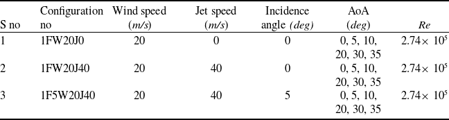
In a single fan configuration, the fan is attached to the baseline wing at the centre of the wing as shown in Fig. 25(a). This bladeless fanjet configuration was tested under the same solver settings with different jet and wind speeds. The operating conditions for the configurations tested are presented in Table 8. The configurations are based on geometric and operating condition of the bladeless fan, e.g. a configuration of 1FW20J40 means single bladeless fanjet at 0 deg (1F), freestream velocity of 20 m/s (W20) and jet velocity of 40 m/s (J40). The CL versus α plot of SFC is compared with BLW and presented in Fig. 28(a). It can be observed that the variation in CL for SFC is small at angles less than 10° AoA; however, at 10° and above, there is a significant improvement in the lift in comparison with BLW (a maximum of 14% increase in the CL_max at 30°). Below 10°, the effect of the bladeless fan on the wing is nullified by the bladeless fanjet itself by creating a negative lift (Fig. 28b). Due to the high-speed jet emanating at the pressure side of the bladeless fanjet aerofoil, the bladeless fanjet produces negative lift till 10° AoA. The stall angle is the same for both the configurations; however, the bladeless fanjet configuration (1FW20J40) shows a gradual stall in comparison with baseline wing (a maximum of 22.5% increase in the CL at 35° - post-stall region).
Operating conditions for single bladeless fanjet configurations

Table 8 Long description
The table presents operating conditions for single bladeless fanjet configurations, focusing on wind speed, jet speed, incidence angle, angle of attack, and Reynolds number. It consists of three rows and six columns. The columns are labeled as follows: Serial number, Configuration number, Wind speed in meters per second, Jet speed in meters per second, Incidence angle in degrees, Angle of Attack in degrees, and Reynolds number. Row 1: Serial number 1, Configuration number 1FW20J0, Wind speed 20 meters per second, Jet speed 0 meters per second, Incidence angle 0 degrees, Angle of Attack 0, 5, 10, 20, 30, 35 degrees, Reynolds number 2.74 times 10 to the power of 5. Row 2: Serial number 2, Configuration number 1FW20J40, Wind speed 20 meters per second, Jet speed 40 meters per second, Incidence angle 0 degrees, Angle of Attack 0, 5, 10, 20, 30, 35 degrees, Reynolds number 2.74 times 10 to the power of 5. Row 3: Serial number 3, Configuration number 1F5W20J40, Wind speed 20 meters per second, Jet speed 40 meters per second, Incidence angle 5 degrees, Angle of Attack 0, 5, 10, 20, 30, 35 degrees, Reynolds number 2.74 times 10 to the power of 5. The table highlights different configurations based on geometric and operating conditions of the bladeless fan, with variations in jet and wind speeds.
Comparison of SFC and BLW: (a) C L and C D versus α; (b) comparison of CL_Fan for SFC with jet ON (1FW20J40) and OFF (1FW20J0) condition.

Figure 28 Long description
A line graph comparing lift coefficient and drag coefficient versus angle of attack for different configurations. The x-axis represents the angle of attack in degrees, ranging from 0 to 40 degrees. The left y-axis represents the lift coefficient, ranging from 0 to 1. The right y-axis represents the drag coefficient, ranging from 0 to 0.6. The graph includes four data series: 1F, 1F with BLW, BLW, and BLW with 1F. Each series is represented by different symbols and line styles. The inset graph (b) compares the lift coefficient of the fan for two conditions: jet ON (1FW20J40) and jet OFF (1FW20J0). The inset graph's x-axis represents the angle of attack in degrees, ranging from 0 to 40 degrees, and the y-axis represents the lift coefficient of the fan, ranging from -0.02 to 0.03. All values are approximated.
Comparison of fan with a preset incidence angle of 5° (IF-5 configuration): (a) C L versus α for BLW, IF and IF-5; (b) exploded view; (c) L/D comparison.

Figure 29 Long description
The image contains three graphs comparing the performance of different fan configurations. Graph (a) is a line graph showing the lift coefficient (C_L) versus angle of attack (AoA) for three configurations: 1F, 1F-5, and BLW. The 1F configuration is represented by black squares, the 1F-5 configuration by red circles, and the BLW configuration by open triangles. The graph indicates that the lift coefficient increases with the angle of attack for all configurations, with the 1F-5 configuration showing the highest lift coefficient at higher angles. Graph (b) provides an exploded view of the lift coefficient versus angle of attack for angles between 0 and 5 degrees, highlighting the initial performance differences among the configurations. Graph (c) is a line graph comparing the lift-to-drag (L/D) ratio versus angle of attack for the same three configurations. The L/D ratio peaks around 10 degrees AoA for all configurations, with the BLW configuration showing a higher L/D ratio at angles greater than 10 degrees. The graphs collectively illustrate the performance advantages of the BLW configuration, particularly at higher angles of attack.
Wind tunnel model for 1FW20J40 configuration.

Figure 30 Long description
The image shows a wind tunnel model designed for the 1FW20J40 configuration of a bladeless fan. The model features a smooth, curved surface that represents the Coanda profile, which is essential for directing airflow. The setup is mounted on a sturdy base, allowing for precise testing and analysis of aerodynamic performance. This model is used to study the flow dynamics of annular jets, which are crucial for the efficient operation of bladeless fans in various applications, including aerospace.
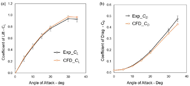
Comparison of experimental and CFD results.

Figure 31 Long description
A line graph compares experimental and computational fluid dynamics results for lift and drag coefficients against angle of attack. The x-axis represents the angle of attack in degrees, ranging from 0 to 40 degrees. The left y-axis represents the lift coefficient, ranging from 0 to 1. The right y-axis represents the drag coefficient, ranging from 0 to 0.6. The graph includes four data lines: experimental lift coefficient, experimental drag coefficient, computational fluid dynamics lift coefficient, and computational fluid dynamics drag coefficient. The experimental lift coefficient is represented by black squares, the experimental drag coefficient by black open squares, the computational fluid dynamics lift coefficient by red triangles, and the computational fluid dynamics drag coefficient by red open triangles. All values are approximated.
Comparison of TFC and DFC with SFC: (a) lift coefficient versus α; (b) drag coefficient versus α.

Figure 32 Long description
The image contains two line graphs. The first graph (a) plots the lift coefficient (C L) against the angle of attack (AoA) in degrees. The second graph (b) plots the drag coefficient (C D) against the angle of attack (AoA) in degrees. Each graph includes three data lines representing different fan configurations labeled as 1F, 2F, and 3F. In graph (a), the lift coefficient increases with the angle of attack for all configurations, with 3F showing the highest values, followed by 2F and 1F. In graph (b), the drag coefficient also increases with the angle of attack, with similar trends across the configurations. All values are approximated.
Comparison of pressure profile of TFC with SFC and DFC at 10° AoA.

Figure 33 Long description
The image contains six line graphs arranged in a two-by-three grid. Each graph compares the pressure coefficient (CP) along a location in feet (ft) for different configurations: TFC, SFC, and DFC at a 10-degree angle of attack. The x-axis represents the location in feet, ranging from 0 to 1.0 or 0.7, depending on the graph. The y-axis represents the pressure coefficient, ranging from -2.0 to 1.5. Each graph uses different colors and symbols to represent data series for 1F, 2F, and 3F configurations at varying conditions. The graphs show how the pressure coefficient varies along the location for each configuration, highlighting differences in pressure profiles. All values are approximated.
Pressure contours of DFC at: (a) 3.5-inch; (b) mid-span; (c) 8.5-inch; (d) quarter-chord.

Figure 34 Long description
A heat map showing pressure contours of a DFC at different span positions. The heat map consists of four subplots labeled (a) through (d), each representing different span positions: 3.5-inch, mid-span, 8.5-inch, and quarter-chord. The color scale at the bottom ranges from blue to red, indicating varying pressure values. Blue represents lower pressure, while red indicates higher pressure. Each subplot shows the distribution of static pressure around an object, with distinct patterns and gradients visible. Subplot (a) shows a concentrated area of high pressure near the object, while subplot (d) displays a more spread-out pressure distribution. The heat map provides a visual representation of how pressure varies across different span positions of the DFC.
Pressure contours for TFC at: (a) 2.5-inch; (b) 5.0-inch; (c) 7.5-inch; (d) quarter-chord at 10°; (e) quarter-chord at 20°; (f) quarter-chord at 35°.

Figure 35 Long description
A heat map displays pressure contours for TFC at different positions. The map includes six subplots labeled (a) through (f), each representing different measurement points: 2.5-inch, 5.0-inch, 7.5-inch, quarter-chord at 10, quarter-chord at 20, and quarter-chord at 35. The color scale ranges from blue to red, indicating varying pressure levels. Higher pressure areas are marked in red, while lower pressure areas are in blue. Each subplot shows the distribution of pressure around a bladeless fan, with noticeable variations in pressure contours at different positions. The heat map provides a detailed visualization of how pressure changes across different points in the fan's operation.
The coefficient of drag is also compared, as shown in Fig. 28(a). The drag for SFC is slightly higher than BLW. The effect is more evident beyond the stalling angle (∼16% increase in drag at 35° - post-stall region). The reasons for higher drag are associated with interference drag created due to fan attachments and additional skin friction and pressure drag due to presence of bladeless fan.
To balance out the negative lift produced by the fan, a preset incidence angle of 5° was given to the bladeless fan. With the increase in fan’s lift due to positive orientation, the overall lift of the configuration increased from the basic fan configuration by approx. 7% as presented in Fig. 29(a). The L/D ratio is also improved and even higher from BLW at an angle greater than 10° AoA.
5.3 Experimental verification of SFC
A baseline experimental model was fabricated with a single bladeless fanjet installed at the mid (Fig. 30). The dimensions were kept similar to the 1FW20J40 configuration (single bladeless fanjet, freestream 20 m/s, fanjet 40 m/s). The model was tested in the low-speed wind tunnel for the calculation of aerodynamic forces. A low-pressure compressor was connected to the model through a mass flow calibrator to ensure an average velocity of 40 m/s at the jet slit. The tunnel speed was set to 20 m/s for tests. The test readings after necessary tunnel corrections (refer to Appendix A) are presented in Fig. 31. A maximum error of 5% was recorded in the lift values and 12% in the drag values. The reason for the higher error in drag values is attributed to the experimental model fabrication tolerance and surface finish.
5.4 Double & triple bladeless fanjet configurations
In a double bladeless fanjet configuration, the fanjets are installed at 3.5 and 8.5 inches from the wing tip, as shown in Fig. 25(d). Similarly, in the triple fanjet configuration, the fanjets are installed at 3, 6 and 9 inches from the wing tip, as shown in Fig. 25(f).
The cases for dual fan configuration (DFC) and triple fan configuration (TFC) were simulated for the entire range of AoAs and the results were compared with SFC (Fig. 32). The results of TFC are better than SFC and DFC because of the resulting pressure profile developed on the wing by triple fanjets (Fig. 33). As can be observed in the chordwise and spanwise distribution, ΔP for TFC is more as compared to SFC and DFC (∼22% increase in lift for TFC over SFC). Figures 34 and 35 presents pressure contours at various chordwise and spanwise locations for DFC and TFC, respectively.
The TFC was compared with the BLW as shown in Fig. 36. Although the lift of TFC is much higher as compared to BLW (approx. 45% increase in lift), the overall L/D ratio is still lower than BLW in pre-stall condition mainly due to increment in skin friction and pressure drag due to presence of additional fan surfaces.
6.0 Integration with aircraft
The bladeless fans effectively modified the wing flow field to improve the lift and reduce the pressure drag; however, overall drag is higher in the pre-stall region for all the configurations as compared to the baseline wing (Fig. 36a). The fan configuration has the potential to replace the propellers on conventional aircraft. The elimination of propeller and associated hardware is going to reduce the overall drag of the aircraft. Thus, to establish the wholesome picture, it was imperative to carry out and compare the results of wind tunnel tests for a propeller UAV and a modified fan configuration of UAV. In the pretext, a CAD model of an existing Radio Control UAV, available with the Aerospace Vehicle Design Lab, CAE, was used to manufacture wind tunnel models for conventional and bladeless UAVs. The bladeless model was modified by incorporating triple fanjets on the upper surface of the UAV. Both models were tested under the same operating conditions i.e. 20 m/s free stream, 40 m/s jet velocity for the bladeless UAV, etc.
The results were compared for both configurations and are presented in Fig. 37. It can be observed that results are comparable in the pre-stall region and better in the post-stall region. Although no design cycle was performed for a bladeless UAV, it still produced comparable results in the pre-stall region. Thus, a properly designed bladeless UAV based on a conceptual design cycle would perform much better than the currently modified UAV, further increasing the margin between conventional and bladeless UAVs.
Comparison of TFC with BLW: (a) C L and C D versus AoA; (b) L/D versus AoA.

Figure 36 Long description
The two line graph compares the lift coefficient and drag coefficient versus angle of attack for two different geometries, Eppler-473 and NACA0012. The x axis represents the angle of attack in degrees, ranging from 0 to 40 degrees. The y axis on the left represents the lift coefficient, ranging from 0 to 1.2. The y axis on the right represents the drag coefficient, ranging from 0 to 0.6. The graph shows two sets of data for each geometry: one for the bladeless fan and one for the baseline wing. The lift coefficient for the bladeless fan increases steadily with the angle of attack, reaching a maximum at around 35 degrees. The lift coefficient for the baseline wing also increases with the angle of attack but at a slower rate, reaching a maximum at around 25 degrees. The drag coefficient for both geometries increases with the angle of attack, with the bladeless fan having a slightly higher drag coefficient than the baseline wing at all angles of attack. All values are approximated.
Wind tunnel testing of conventional and modified bladeless UAV: (a) bladeless UAV; (b) conventional UAV; (c) C L versus C D ; (d) C L /C D versus AoA.

Figure 37 Long description
The image contains two photos and two diagrams side by side. The photos show two different unmanned aerial vehicles (UAVs) in a wind tunnel. The first photo (a) displays a bladeless UAV with a streamlined nose and fanjets on the wings. The second photo (b) shows a conventional UAV with a propeller installed on the nose. The diagrams present performance data. Diagram (c) plots the lift coefficient (C L) against the drag coefficient (C D) for both UAVs, with the bladeless UAV represented by red dots and the conventional UAV by black squares. Diagram (d) shows the ratio of lift to drag coefficient (C L /C D) versus the angle of attack (AoA) for both UAVs, using the same color scheme. The data indicates differences in aerodynamic performance between the two UAV designs.
7.0 Conclusion
A detailed computational analysis was presented for semi-annular bladeless fan configurations to evaluate the effect of fanjet height, spanwise and chordwise location, orientation and number of bladeless fan units on the aerodynamic performance of the baseline wing. The aerodynamic efficiency (lift/drag ratio) of leading-edge fanjet configurations was better than the trailing-edge configurations and showed better flow control in the post-stall region. Leading-edge configurations with higher radii also produce more net propulsive force as compared to other configurations and were selected for further analysis from integration perspective with aircraft wing.
During analysis, it was revealed that fanjets were effective in modifying the flow field across the wing and produced higher lifts; however, the configuration also offered more drag as compared to the baseline wing. The additional bladeless fan surfaces and the interaction of high-speed jet with these surfaces contributed towards skin friction drag, thus increasing the overall drag for the configurations. The interference created by the integration of finite semi-annular fanjets over the baseline wing was also a major contributor toward the higher drag. Out of the tested bladeless fan configurations, the triple-fanjet configuration was better than others because more area was influenced by the presence of fanjets as compared to single and dual fanjets. An increase of 45% was observed for TFC over baseline wing with ∼16% increase in drag in post stall region (at 35° AoA). The preset positive incidence angle of the bladeless fan further improves the aerodynamic efficiency of the wings (∼7% additional increase in the lift over parent configuration). The positive incidence for the fanjet ensures positive lift created by the fanjet itself. Moreover, the jet orientation toward the surface of the baseline wing further helps in keeping the flow attached to the surface in post-stall condition.
The bladeless fanjets would replace the propellers and their drive system from the conventional propeller-driven small aircraft/ UAV. The elimination of a propeller and engine would render a smooth aircraft profile, reducing overall drag for the aircraft. Therefore, to establish the wholesome picture, wind tunnel testing of a baseline propeller UAV and a modified version of the UAV were carried out. The aerodynamic efficiency was better for the modified configuration as compared to the baseline model (a maximum of ∼20% increase in lift for the same drag count); thus, the fanjet configuration has the potential to further improve the aerodynamic efficiency, if properly designed by adopting established design cycle procedures.
8.0 Future work
Keeping in view of the outcome of the present work, the following areas will be explored in future:
-
(a) Comprehensive computational and experimental studies may be conducted for shapes other than semi-annular.
-
(b) Comparison of Weight and energy requirement may be done for bladeless fanjets system with equivalent propulsion system for generation of similar performance parameters on similar platforms.
-
(c) A UAV based on fanjets may be designed and built using established design cycles to analyse the overall aerodynamics of the configuration.
Competing interests
The authors have no competing or conflict of interest.
Appendix A Wind tunnel setup
For the present research work, wind tunnel experiments were conducted in a 2-ft × 3-ft rectangular cross-section wind tunnel facility held at the College of Aeronautical Engineering, NUST. It is a closed-circuit, closed-test section, horizontal-type wind tunnel, capable of producing 110 m/s air flow in the test section. The wind tunnel is equipped with a 150-HP motor for driving variable pitch propeller at a max RPM of 1,500. The flow conditioning is achieved through a diffuser, stilling chamber and contraction section. A honeycomb and stilling structure upstream of test section reduces the turbulence levels. A fixed contour subsonic converging nozzle accelerates the flow into the rectangular test section. As the geometry is fixed, the desired velocity in the test section is controlled by adjusting the propeller pitch using an electric controller. Along with wind tunnel speed control, the operator can remotely control pitch (± 30°) and yaw attitudes (± 90°) of the model. The aerodynamic forces and moments are measured using three-axis pyramidal balance with the help of three struts directly connected with the balance and used to hold the model in the test section (two forward and one rear attachment). Before proceeding with the experiments, the following calibrations were performed.
Velocity calibration. The velocity in the test section is measured using an air meter (inclined manometer based on methyl alcohol with a specific gravity of 0.812 at STP). The air meter is connected to a total pressure port located in the stilling chamber and static pressure port in the test section. The air meter indicates the speed in miles per hour. The wind tunnel speed shown by air meter was calibrated against a pitot static tube mounted in the test section. Error analysis of the complete system was conducted including mechanical errors and instrumental accuracy. A true velocity versus air meter indicated velocity is plotted for reference with error bars shown in Fig. A1(a). In reduction of data of the pitot static tube, compressibility effects were neglected due to low air velocities. The calibration runs were conducted for wind tunnel speed ranging from 10 mph (4.47 m/s) to 50 mph (22.35 m/s).
(a) Velocity calibration charts. The velocity indicated by air meter was compared with the true velocity captured by pitot-static sensor. The error analysis was also conducted based on instrumentation and mechanical errors and represented by error bars. (b) AoA calibration plot between true AoA and angle shown on WTT console. The error analysis of the complete system was conducted including instrumentation errors etc. and represented on the plot in the form of error bars.

Figure A1 Long description
The line graph presents the calibration of velocity in a test section, comparing true velocity measured by a pitot-static sensor with the velocity indicated by an air meter. The x-axis represents the velocity indicated by the air meter in meters per second, ranging from 0 to 25 meters per second. The y-axis represents the true velocity in meters per second, also ranging from 0 to 25 meters per second. The data points show a linear relationship between the true velocity and the air meter indicated velocity, with error bars representing the error analysis of the complete system, including mechanical errors and instrumental accuracy. The graph demonstrates that the true velocity closely matches the velocity indicated by the air meter, with minor deviations shown by the error bars. All values are approximated.
AoA calibration. The AoA of the model is directly controlled by the operator through electrical actuation of the rear attaching struct. The achieved AoA is displayed on the console in the control station connected with the data acquisition system. The AoA calibration was conducted against WTT horizontal axis using an inclinometer placed on the top of the model. The readings from the console and inclinometer were recorded and are presented in Fig. A1(b). Flow angularity was measured using WTT runs with the model installed. The complete data was analysed for error computations. The errors include instruments error, flow angularity due to solid, wake, strut etc. The true AoA versus indicated AoA on console is presented below with error bars. The AoA during wind tunnel experiments varied from 0 to +35°.
Pyramidal balance calibration. The pyramidal balance uses six strain of gauges to measure forces and moments. Before test runs, the balance calibration was conducted using a standard procedure to determine balance interactions and calibration slopes. Known weights were put on the TEE assembly connected to balance in all three forces and moments directions. Loads were progressively added and then removed in one direction, and readings (three forces and three moments) were noted from data acquisition system, thus the effect of each force or moment on remaining forces and moments were determined; e.g. the slope of Data Acquisition (DAQ) readings versus applied loads were calculated and arranged in the form of a calibration matrix, which is used to correct the test run results, as shown below:
 \begin{align*} \left[ {\begin{array}{*{20}{c}}{\dfrac{{\partial LFR}}{{\partial LF}}}\quad{\dfrac{{\partial LFR}}{{\partial DF}}}\quad{\dfrac{{\partial LFR}}{{\partial SF}}}\quad{\dfrac{{\partial LFR}}{{\partial PF}}}\quad{\dfrac{{\partial LFR}}{{\partial YF}}}\quad{\dfrac{{\partial LFR}}{{\partial RF}}}\\[12pt]{\dfrac{{\partial DFR}}{{\partial LF}}} \quad {\dfrac{{\partial DFR}}{{\partial DF}}}\quad{\dfrac{{\partial DFR}}{{\partial SF}}}\quad{\dfrac{{\partial DFR}}{{\partial PF}}}\quad{\dfrac{{\partial DFR}}{{\partial YF}}}\quad{\dfrac{{\partial DFR}}{{\partial RF}}}\\[12pt]{\dfrac{{\partial SFR}}{{\partial LF}}}\quad {\dfrac{{\partial SFR}}{{\partial DF}}}\quad{\dfrac{{\partial SFR}}{{\partial SF}}}\quad{\dfrac{{\partial SFR}}{{\partial PF}}}\quad {\dfrac{{\partial SFR}}{{\partial YF}}}\quad{\dfrac{{\partial SFR}}{{\partial RF}}}\\[12pt]{\dfrac{{\partial PMR}}{{\partial LF}}}\quad {\dfrac{{\partial PMR}}{{\partial DF}}}\quad{\dfrac{{\partial PMR}}{{\partial S}}}\quad{\dfrac{{\partial PMR}}{{\partial PM}}}\quad{\dfrac{{\partial PMR}}{{\partial YM}}}\quad {\dfrac{{\partial PMR}}{{\partial RM}}}\\[12pt]{\dfrac{{\partial YMR}}{{\partial LF}}}\quad {\dfrac{{\partial YMR}}{{\partial DF}}}\quad{\dfrac{{\partial YMR}}{{\partial SF}}}\quad{\dfrac{{\partial YMR}}{{\partial PM}}}\quad{\dfrac{{\partial YMR}}{{\partial YM}}}\quad{\dfrac{{\partial YMR}}{{\partial RM}}}\\[12pt]{\dfrac{{\partial RMR}}{{\partial LF}}}\quad {\dfrac{{\partial RMR}}{{\partial DF}}}\quad{\dfrac{{\partial RMR}}{{\partial SF}}}\quad{\dfrac{{\partial RMR}}{{\partial PM}}}\quad{\dfrac{{\partial RMR}}{{\partial YM}}}\quad {\dfrac{{\partial RMR}}{{\partial RM}}}\end{array}} \right] \end{align*}
where LFR stands for lift force reading (from DAQ) and LF stands for applied load in lift force directions. Similarly, DF is drag force, SF is side force, PM is pitching moment, YM is yawing moment and RM is for rolling moment.
 $\partial LFR /\partial LF $
represents the slope of lift force reading on DAQ versus applied load in the lift direction, and similarly the rest can be defined accordingly.
The diagonal elements represent slopes of calibration curves for lift, drag and side forces, and pitching, yawing and rolling moments, while the off-diagonal terms represent the interaction terms – the effect of one force or moment on rest of the forces and moments. The test run results, once multiplied with the inverse of the calibration matrix, would result in corrected forces and moments for the test run.
Drag force correction. Due to presence of the struts in the test section to hold test models, contribute additional unwanted drag i.e. tare drag due to strut itself and interference drag due to disturbance of the flow. To correct the drag, a two-step approach was followed. First the drag was calculated with the model in an inverted position (Equation (A1)), followed by the addition of a dummy lower strut to the previous configuration (Equation (A2)):
 \begin{align} {D_1} &= {D_{inverted}} + {T_{upper}} + {I_{upper}} \\[-6pt] \nonumber \end{align}
 \begin{align} {D_2} &= {D_{inverted}} + {T_{upper}} + {I_{upper}} + {T_{lower}} + {I_{lower}} \\[10pt] \nonumber \end{align}
where
 ${D_{inverted}}$
is the drag of model in the inverted position,
 ${T_{upper}}$
is the Tare drag of the strut attached with the upper surface of model,
 ${I_{upper}}$
is the interference drag on the upper surface of the model due to the presence of strut,
 ${T_{lower}}$
tare is drag on the lower surface of the model and
 ${I_{lower}}$
is the interference drag on the lower surface of the model. The difference of the two drags will give us the required (
 ${T_{lower}} + {I_{lower}}$
), which is required during Wind Tunnel Testing (WTT) data reduction to capture true test model drag.
Wind tunnel corrections. Wind tunnel correction includes data corrections for horizontal buoyancy, solid blocking, wake blocking, etc. The blockage factor for the tunnel is denoted by ε and is used to correct velocity, dynamic pressure and Re (see Equation (A3), (A4) and (A5)). The subscript ‘u’ represents the uncorrected values, whereas TF represent tunnel turbulence factor. Downwash correction factor τ and boundary correction factor δ were used for streamline curvature correction of forces and moments coefficients e.g. Equation (A6) presents CL correction (similar equations for rest of the forces and moments).
 \begin{align} V &= \;{V_u}\left( {1 + { \in _{sb}} + { \in _{wb}}} \right) \\[-2pt] \nonumber \end{align}
 \begin{align} q &= \;{q_u}\left( {1 + 2\left( {{ \in _{sb}} + { \in _{wb}}} \right)} \right) \\[-2pt] \nonumber \end{align}
 \begin{align} Re &= \;R{e_u}\left( {1 + { \in _{sb}} + { \in _{wb}}} \right) \times TF \\[-6pt] \nonumber \end{align}
 \begin{align} {C_L} &= \;{C_{Lu}}\left( {1 - 2\left( {{ \in _{sb}} + { \in _{wb}}} \right)} \right) - \tau {C_{L\alpha }}\delta \frac{S}{c}{C_{Lu}} \\[10pt] \nonumber \end{align}
The data presented in the paper is the corrected data obtained through the corrections process mentioned above.
CFD simulation setup
Computational domain. The computational domain is presented in Fig. A2.
Computational domain, boundary conditions and domain meshing. Fanjet and bladeless fan have been used interchangeably in this work.

Figure A2 Long description
The diagram illustrates a computational domain with boundary conditions and domain meshing for a bladeless fan and a baseline wing. The domain is enclosed in a rectangular cross-section. The bladeless fan uses an Eppler-473 aerofoil cross-section, while the baseline wing uses a NACA0012 aerofoil cross-section. The diagram includes labels for velocity inlets, pressure outlets, and walls. The velocity inlet jet is positioned near the bladeless fan, and the pressure outlet is located at the far right. The domain is meshed to show the grid used for computational fluid dynamics analysis. The zoomed-in sections highlight the detailed meshing around the aerofoils.
Boundary conditions. The boundary conditions are presented in Table A1.
Boundary conditions (BC) for the computational setup

Note: A jet ratio of 2 is higher than the local velocity ratio
 $\left( {{V_{0.25c}}/{V_\infty }} \right)$
for the computational cases.
Solver setting for simulations: (transient, incompressible, viscous analysis). The solver setting is presented in Table A2.
Extended solver setting for simulation work

Table A2 Long description
A table with three columns labeled Item, Description, and Parameters, and six rows detailing solver settings for simulation work. Row 1: Item, Solver; Description, Pressure-based solver; Parameters, PISO. Row 2: Item, Turbulence model; Description, SST-kw; Parameters, Y+ 1Enhanced wall treatment. Row 3: Item, Spatial discretisation; Description, Second order; Parameters, Upwind scheme. Row 4: Item, Spatial convergence; Description, Residual; Parameters, less than 1e-6. Row 5: Item, Temporal discretisation; Description, Second order; Parameters, Implicit. Row 6: Item, Time step; Description, As per CFL criteria; Parameters, delta t equals 2.5 microseconds. Row 7: Item, Temporal iteration; Description, Iterations per time step; Parameters, 40.
Application of error corrections on performance data
The experimental data were analysed for errors, which are based on instrumental errors, procedural errors, system tolerances, etc. As the lift and drag values are dependent on coefficients, dynamics pressures, AoAs, etc., any error in the correct measurement of these parameters is going to contribute toward the overall errors on the lift and drag values. Similarly, for simulation results the uncertainty in correct prediction of these coefficients were estimated from grid resolution, turbulence modeling and iterative convergence residuals. The CL and CD data with error bars and uncertainty bars are presented in Fig. A3 for the interest of the wider public.
CL and CD versus AoA with errors bars (experimental data) and uncertainty (CFD data).

Figure A3 Long description
Two line graphs compare the coefficient of lift and drag with the angle of attack. The x-axis represents the angle of attack in degrees, ranging from 0 to 40 degrees. The y-axis of the first graph represents the coefficient of lift, ranging from 0 to 1.2, while the y-axis of the second graph represents the coefficient of drag, ranging from 0 to 0.6. Each graph contains two data lines: one for experimental data (Exp_CL and Exp_CD) and one for computational fluid dynamics data (CFD_CL and CFD_CD). The experimental data is represented by black lines with circular markers, and the CFD data is represented by orange lines with square markers. Both graphs show error bars for the experimental data and uncertainty for the CFD data. The coefficient of lift increases with the angle of attack, while the coefficient of drag also increases with the angle of attack. All values are approximated.