

Introduction
Cladonia is one of the most diverse macrolichen genera, with 475 species recognized at present (T. Ahti 2017, pers. comm). The podetium morphology and the surface features, along with the secondary metabolites, have been the characters commonly used for species identification (Ahti Reference Ahti2000). There are no known characters of the hymenium that would be useful to distinguish species and the specimens often appear without apothecia. The problem of identification within the genus Cladonia is particularly aggravated in those groups of species where the primary thallus is dominant and seldom develops podetia, resulting in a very low number of taxonomic characters. In these cases, the morphological characters used for identification are the size and morphology of squamules, the presence of incisions and squamule chemistry (including coloration), but all these characters are strongly affected by habitat conditions (Stenroos et al. Reference Stenroos, Hyvönen, Myllys, Thell and Ahti2002). One such group is composed of the species formerly included in the subsection Foliosae (Mattick Reference Mattick1940), namely C. foliacea, C. convoluta and C. angustiloba. They are characterized by a well-developed primary thallus, with a yellowish-green upper side and yellow lower side, the presence of usnic and fumarprotocetraric acids, often zeorin and the rarely occurring psoromic acid. The problem with distinguishing between C. foliacea and C. convoluta has been studied using morphological (Burgaz et al. Reference Burgaz, Escudero and Ahti1993) and phylogenetic (Pino-Bodas et al. Reference Pino-Bodas, Martin and Burgaz2010) approaches. Despite finding no clear separation in squamule size between C. foliacea and C. convoluta (Burgaz et al. Reference Burgaz, Escudero and Ahti1993), they were still hesitantly recognized as distinct species (Burgaz & Ahti Reference Burgaz and Ahti2009). The phylogenetic analyses by Pino-Bodas et al. (Reference Pino-Bodas, Martin and Burgaz2010) did not find any phylogenetic lineage associated with the traditional circumscription of C. foliacea and C. convoluta, concluding that the phenotypic variation observed is most likely an adaptive response to different environmental conditions, such as substratum type or degree of aridity. Ahti & Stenroos (Reference Ahti and Stenroos2013) included C. convoluta in C. foliacea but some authors have still retained them as separate species (Çobanoğlu & Sevgi Reference Çobanoğlu and Sevgi2012; Bendaikha & Hadjadj-Aoul Reference Bendaikha and Hadjadj-Aoul2016; Catalano et al. Reference Catalano, Mingo, Migliozzi and Aprile2016; Christensen Reference Christensen2016). Cladonia angustiloba Ahti & Aptroot is a species very similar to C. foliacea, from which it can be separated by having very narrow squamules with deep incisions (Ahti & Aptroot Reference Ahti and Aptroot2009). It was described as endemic to Macaronesia (Ahti & Aptroot Reference Ahti and Aptroot2009) but it has subsequently been found in the Faroe Islands (Denmark) (Ahti & Stenroos Reference Ahti and Stenroos2012), Scotland and Ireland (B. J. Coppins 2016, pers. comm.). However, no molecular studies have been conducted to date in order to determine whether this species is an independent lineage. Owing to the large variation shown by the species within this genus (as seen in the C. foliacea/C. convoluta complex) and to the large number of polyphyletic species comprising the genus Cladonia (e.g. Stenroos et al. Reference Stenroos, Hyvönen, Myllys, Thell and Ahti2002; Steinová et al. Reference Steinová, Stenroos, Grube and Škaloud2013; Pino-Bodas et al. 2015 Reference Pino-Bodas, Burgaz, Martín, Ahti, Stenroos, Wedin and Lumbscha ), it was necessary to check by means of DNA sequences whether C. angustiloba is a separate species. We also included additional specimens of C. convoluta and C. foliacea s. str. in our analyses.
The aim of this work was to study the circumscription of C. angustiloba using two nuclear loci, ITS rDNA and RPB2, and one mitochondrial locus, cox1, together with species delimitation methods.
Material and Methods
Taxon sampling
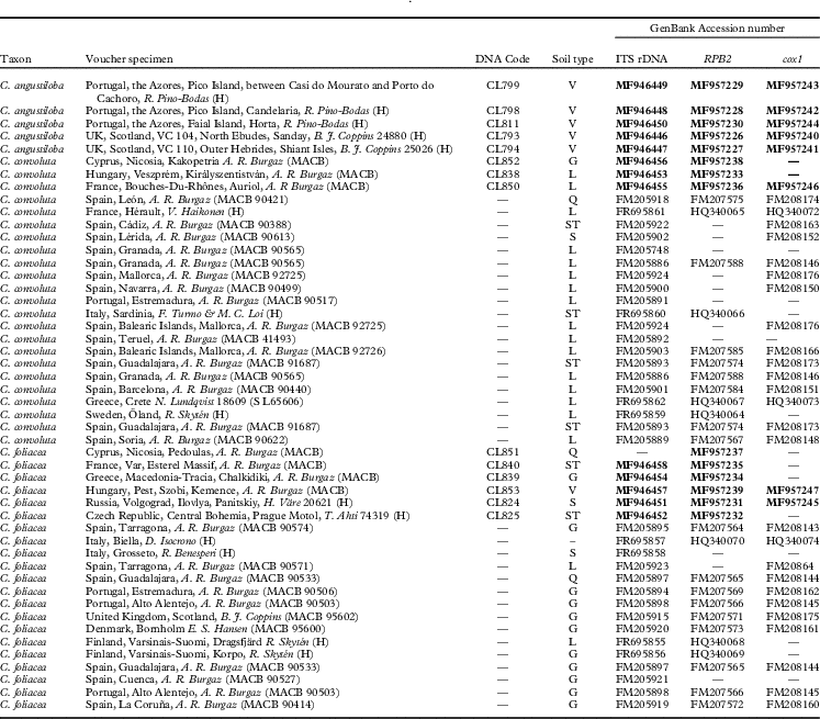
Fourteen new specimens were sequenced, five of Cladonia angustiloba, six of C. foliacea and three of C. convoluta (Table 1). The new specimens of C. foliacea and C. convoluta came from geographical areas poorly represented in the earlier molecular study (Pino-Bodas et al. Reference Pino-Bodas, Martin and Burgaz2010), such as the Czech Republic, Cyprus, France, Greece, Hungary and Russia. The specimens of C. angustiloba came from two islands in the Azores (one of them close to the type locality) and from Scotland (two specimens). The same loci used in the previous work by Pino-Bodas et al. (Reference Pino-Bodas, Martin and Burgaz2010) were studied here: ITS rDNA, RPB2 and cox1. Pino-Bodas et al. (Reference Pino-Bodas, Martín, Burgaz and Lumbsch2013) found that RPB2 and cox1 are suitable loci to delimit species in Cladonia. Cladonia cariosa, C. cervicornis and C. firma were selected as outgroup according to Pino-Bodas et al. (Reference Pino-Bodas, Martín, Burgaz and Lumbsch2013). The specimens were studied under an Olympus SZX9 dissecting microscope and an Olympus CX42 microscope. The secondary metabolites of each specimen were analyzed by thin-layer chromatography (TLC) according to standardized procedures (White & James Reference White and James1985; Orange et al. Reference Orange, James and White2001), using the solvents A, B and C.
Specimens of the Cladonia foliacea complex used in this study together with localities, GenBank Accession numbers and soil types. DNA codes correspond to our laboratory codes, which are indicated in the phylogenetic tree (Fig. 1). New sequences are in bold

Type of soil: L=limestone, Q=quartzite, G=granite, ST=sandstone, S=sandy soil, V=volcanic rocks
DNA extraction, PCR and sequencing
Secondary metabolites were extracted by soaking the samples in acetone for 2 h prior to DNA isolation. The E.Z.N.A. Forensic DNA Isolation Kit (Omega Bio-Tek) was used to extract the genomic DNA. The DNA was eluted in 100 µl of elution buffer included in the kit. PCRs were carried out with Ready-to-Go-PCR Beads (GE Healthcare Life Sciences, UK). The volume of reaction was 25 µl for each tube, with 1 µl of each primer at 10 μM concentration, 3 µl of DNA, 2·5 units of PuReTaq DNA Polymerase, a concentration of 200 mM of dNTP and 1·5 mM of MgCl2. The primers used to amplify each locus and the PCR programs used are described in Pino-Bodas et al. (Reference Pino-Bodas, Martin and Burgaz2010). PCR products were cleaned with ExoProStarTM 1-step (GE Healthcare). The Sanger sequencing reactions were performed at Macrogen Europe (www.macrogen.com) with the same primers used for the PCR.
The program Sequencher 4.1.4 (Gene Codes Corporation, Ann Arbor, Michigan, USA) was used to assemble the sequences. All sequence alignments were performed using MAFFT (Katoh & Standley Reference Katoh and Standley2013), then they were checked and improved manually in BioEdit 7.0 (Hall Reference Hall1999). The intron at the 3' end of 18S and 9-nucleotide tandem repeat motif of cox1 were removed from the alignments. The ambiguous regions were removed using Gblocks 0.91b (Castresana Reference Castresana2000) with the less stringent option, keeping 88% of the original positions.
Phylogenetic analyses
Each region was analyzed by maximum likelihood (ML). The ML analyses were implemented using RAxML (Stamatakis Reference Stamatakis2006) assuming the GTRGAMMA model. The bootstrap searches were conducted with 1000 pseudoreplicates using the rapid bootstrap algorithm. Congruence among the different topologies inferred from the loci was tested following Lutzoni et al. (Reference Lutzoni, Kauff, Cox, McLaughlin, Celio, Dentinger, Padamsee, Hibbett, James and Baloch2004). We consider nodes to be in conflict if different topologies are each supported with at least 75% bootstrap. The positions of three specimens were incongruent between ITS rDNA and RPB2 datasets, and these samples were removed from the combined dataset. The combined dataset was analyzed by ML and Bayesian inference. The ML was run using the GTRGAMMA model with five partitions (cox1, ITS and each codon position of RPB2). Two different analyses were run: 1) all specimens included (specimens with one, two or three loci); 2) complete matrix, only the specimens with at least two loci included. The results of both analyses were similar and the Bayesian analysis was run only for the complete matrix. The substitution model for each locus was selected with jModelTest (Posada Reference Posada2008) using the Akaike Information Criterion (AIC). The models selected were: TPMfuf for cox1, TrNef+I for ITS and TIM2ef+I for RPB2. The Bayesian analysis was carried out using MrBayes 3.2.6 (Ronquist et al. Reference Ronquist, Teslenko, van der Mark, Ayres, Darling, Hohna, Larget, Liu, Suchard and Huelsenbeck2012) using five partitions and with jModelTest selected models except for the RPB2 partitions. TIM2ef+I is not implemented in Mr Bayes and was replaced by GTR+I according to Huelsenbeck & Rannala (Reference Huelsenbeck and Rannala2004). Two simultaneous runs with 20 000 000 generations, each one starting with a random tree and employing four simultaneous chains, were executed. Every 1000th tree was saved. After the analysis, the convergence between runs was checked using the average standard deviation of split frequencies (it was below 0·005) and by plotting likelihood values across generations using Tracer 1.5 (Rambaut & Drummond Reference Rambaut and Drummond2009). The first ten million generations were discarded as burn-in and the 50% majority-rule consensus tree was calculated using the ‘sumt’ command of MrBayes.
Polymorphisms and genetic differentiation
The number of fixed nucleotide differences, number of shared polymorphic positions and the pairwise fixation indices (F st ) between the species were estimated in DnaSP v5. (Librado & Rozas Reference Librado and Rozas2009).
Species delimitation analyses
According to Carstens et al. (Reference Carstens, Pelletier, Reid and Satler2013), several analytical methods must be used in order to delimit species. Three “discovery” species delimitation methods were used to infer the species in the Cladonia foliacea complex: the General Mixed Yule Coalescent (GMYC) approach (Pons et al. Reference Pons, Barraclough, Gomez-Zurita, Cardoso, Duran, Hazell, Kamoun, Sumlin and Vogler2006), the Poisson Tree Processes (PTP) method (Zhang et al. Reference Zhang, Kapli, Pavlidis and Stamatakis2013) and the automatic barcode gap (ABGD) method (Puillandre et al. Reference Puillandre, Lambert, Brouillet and Achaz2012). GMYC is a likelihood method that uses the different branching patterns of an ultrametric gene tree to establish the transition point between inter- and intra-species branching rates. GMYC analyses were run in R using the splits package (http://r-forge.r-project.org/projects/splits/). Single threshold and multiple threshold models were tested. The single threshold model defines a transition from species to population level in an ultrametric tree, the nodes before the transition reflect speciation events and the nodes after the transition reflect coalescence within species. Once this boundary is reached, the multiple threshold model searches alternative models that iteratively split and unite the species clusters. The log-likelihood ratio test (LTR) was used to compare the alternative model (specimens are divided into n species) with the null model (all specimens belong to a single species). The analyses were run for each dataset (ITS rDNA, cox1, RPB2 and the combined dataset including only the specimens with three loci). The outgroup was included in the analyses. The ultrametric trees for GMYC were generated in BEAST 1.8 (Drummond et al. Reference Drummond, Suchard, Xie and Rambaut2012) under an uncorrelated lognormal clock and with a coalescent model of constant population size. The analysis was run for 50 000 000 generations and sampled every 1000. The convergence was calculated with Tracer 1.5. After discarding the first 5 000 000 generations the effective sample size for all the parameters of the evolutionary model reached values>200. The tree was summarized with TreeAnnotator 1.7.5 (Rambaut & Drummond Reference Rambaut and Drummond2013) using the maximum clade credibility tree option for the target tree type. PTP is similar to the GMYC method but uses the number of substitutions instead of the branching rates to delimit the species. Some studies have demonstrated that this method gives more robust results than GMYC (Zhang et al. Reference Zhang, Kapli, Pavlidis and Stamatakis2013; Ortiz & Francke Reference Ortiz and Francke2016). PTP analyses were run using the best ML trees from RAxML analyses for single locus. The analyses were implemented in the webserver (http://species.h-its.org/) for 500 000 generations, thinning=100 and 10% of burn-in. The ABGD approach is based on the distribution of genetic pairwise distances to detect the “barcode gap”. ABGD was used to detect the barcode gap in the ITS rDNA dataset, the barcode marker for fungi (Schoch et al. Reference Schoch, Seifert, Huhndorf, Robert, Spouge, Levesque and Chen2012). This analysis was conducted in the webserver (http://www.abi.snv.jussieu.fr/public/abgd/) with default parameter: Jukes-Cantor (JC69) model was used to calculate the genetic distances, Pmin=0·001, Pmax=0·1, step=10 and Nb bins=20.
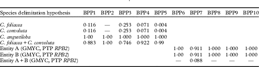
After these analyses, a Bayesian phylogenetic and phylogeography (BPP) method (Rannala & Yang Reference Rannala and Yang2003) and Bayes factor (Leaché et al. Reference Leaché, Fujita, Minini and Bouckaert2014) were used to validate the species delimitation hypotheses obtained from the discovery methods. BPP was run using the program BPP v. 3.3 (Yang & Rannala Reference Yang and Rannala2014; Yang Reference Yang2015) using “A11” algorithm (Yang Reference Yang2015). The analyses were run with different sets of priors for population size (θ) and the age of the root in the species tree (τ) (Table 5) and automatic fine-tune adjustments of the parameters. Each analysis was run for 200 000 generations, sampled every 2 generations and the first 10% were discarded as burn-in. Owing to the fact that the analysis permits grouping different species into one, but does not permit the division of the predefined species, the analyses were carried out with two different criteria in order to assign individuals to species. In the first one (BPP1–BPP5 analyses in Table 5) the specimens were assigned to the traditionally accepted species (C. foliacea, C. convoluta, C. angustiloba). In the second, the specimens were assigned to two possible species (BPP6–BPP10 analyses in Table 5) as suggested by some of the species delimitation analyses (GMYC and PTP for RPB2); these were called “entity A” and “entity B”.
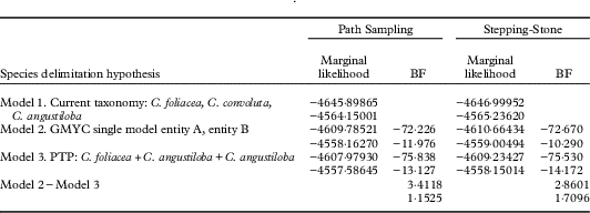
Bayes factor uses a Bayesian coalescent-based reconstruction of species trees to compare the different species delimitation models, calculating the marginal likelihood, and does not require a guide tree. This method was used to compare the different species delimitation models produced by other methods: Model 1, with the three current species, C. foliacea, C. convoluta and C. angustiloba; Model 2 with two species morphologically cryptic (supported in several of the GMYC analyses), entity A and entity B; Model 3 with only one species in the C. foliacea complex (supported by PTP results of ITS rDNA and cox1; results of GMYC single threshold for ITS rDNA and cox1; and ABGD). Marginal likelihood for each competing model was estimated using path sampling (PS) and stepping-stone sampling (SS) in *BEAST. The analyses were run with the same substitution models used in MrBayes, under a strict clock for each locus, the Yule process model and constant population size for species tree priors. The MCMC chain was run for 200 000 000 generations and sampled every 2000th generation. The effective sample size (ESS) was evaluated in Tracer 1.5 and all the values were >200. Bayes factor is calculated as 2×(marginal likelihood Model 1 – marginal likelihood Model 2). Negative values of Bayes factor support Model 1 and positive values support Model 2. To explore the effect of missing data on Bayes factor results, we ran the analyses with the combined dataset of at least two loci, and with the complete combined dataset in which all the specimens had sequences of three loci.
Results
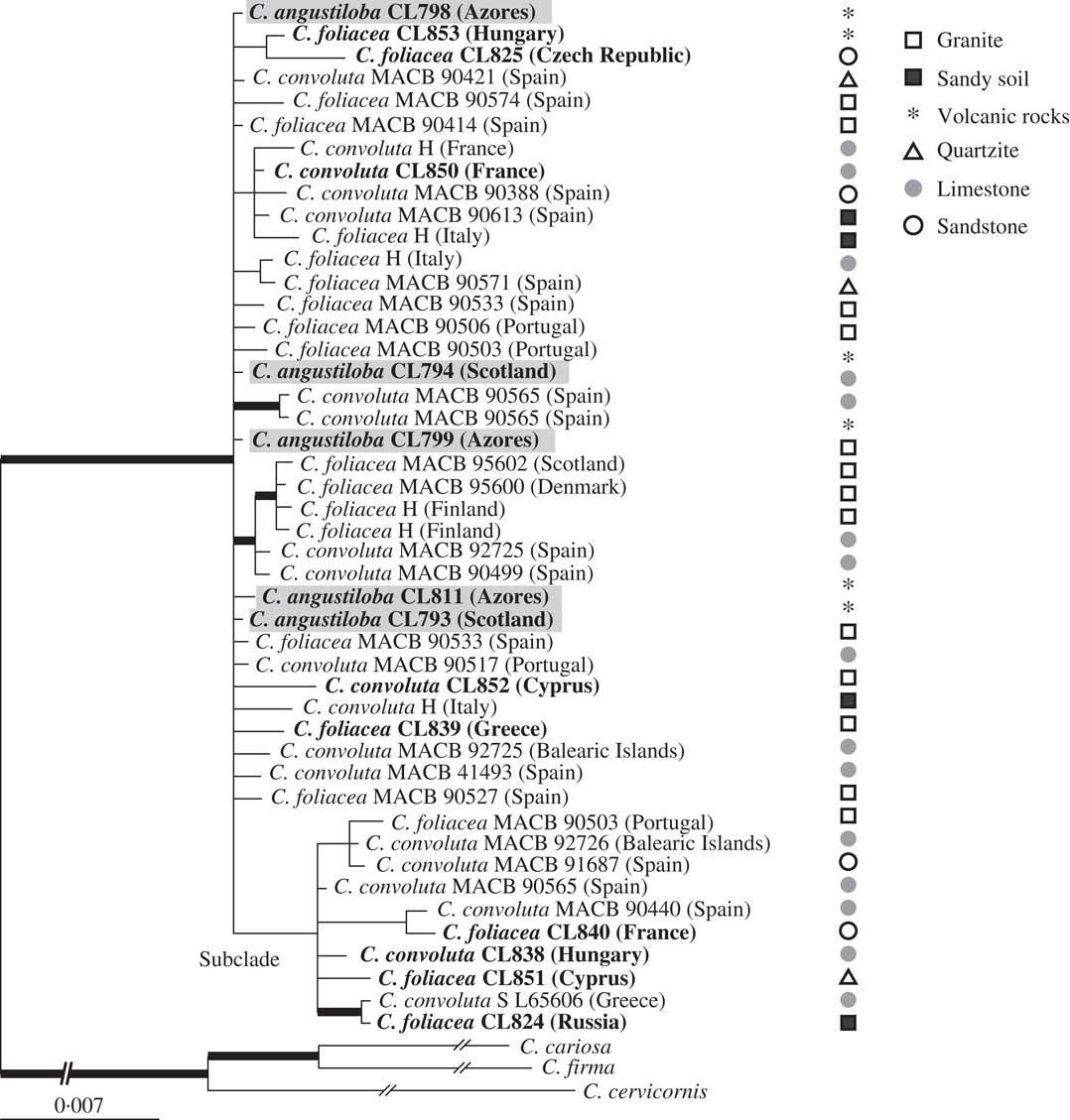
In this study, 35 new sequences have been generated (13 of ITS rDNA, 14 of RPB2 and 8 of cox1) (Table 1). The alignments for the respective loci contained 52 sequences and 589 positions for ITS rDNA, 40 sequences and 1045 positions for RPB2, and 39 sequences and 717 positions for cox1. The concatenated dataset contained 49 sequences and 2080 characters, 128 of which were parsimony-informative. The ML analysis from the concatenated dataset yielded a tree with −Lnl=4354·334 and the Bayesian analysis yielded a tree with an arithmetic mean of −Lnl=4576·602. The tree topology from both analyses was similar; the 50% majority tree from the Bayesian analysis is shown in Fig. 1. The three species were polyphyletic. A well-supported clade comprised the specimens representing the three species C. angustiloba, C. convoluta and C. foliacea. This clade contained one unsupported subclade which contained specimens from C. convoluta and C. foliacea from different geographical regions (Fig. 1). In the ML analysis all the specimens of the C. foliacea complex formed a well-supported clade. This clade was split into two unsupported subclades (data not shown), each one containing specimens of more than one described species.
Phylogeny of the Cladonia foliacea group based on a combined dataset (ITS rDNA, RPB2 and cox1) with substratum type. This is a 50% majority-rule consensus tree of a Bayesian analysis. Branches supported with bootstrap >70% and posterior probability >0·95 are indicated by thick black lines. Newly sequenced specimens indicated in bold, remainder of sequences taken from Pino-Bodas et al. (Reference Pino-Bodas, Martin and Burgaz2010). Cladonia angustiloba specimens are highlighted in grey. Cladonia cariosa, C. cervicornis and C. firma are used as outgroups.

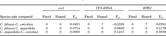
Table 2 shows the genetic divergence between the species. No fixed nucleotide differences were found between them. The F st values were close to zero, indicating no genetic differentiation between the species.
Number of fixed differences (Fixed), number of shared polymorphisms (Shared) and fixation indices (FST) for three gene loci for the species included in the Cladonia foliacea complex

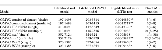
The results of the GMYC analyses are summarized in Table 3. The multiple threshold analyses delimit a higher number of species than the single threshold analyses, with the exception of RPB2 (same number of species delimited in both cases). The single threshold analyses of ITS rDNA and cox1 (the latter is not significant) revealed the existence of a unique species in the C. foliacea complex, and three more corresponding to the outgroup. The analyses of RPB2 (single and multiple threshold) and the single threshold analyses of the combined matrix inferred two species for the C. foliacea complex, one corresponding to the subclade found in the phylogenetic analyses, another corresponding to the remaining specimens.
Species delimitation analyses for the Cladonia foliacea complex using the GMYC (General Mixed Yule Coalescent) method with single and multiple threshold models. Number of ML (maximum likelihood) entities represents the number of putative species delimited by this method (confidence interval). The analyses included the three outgroup species

Log-likelihood ratio test: ** P<0·01, * P<0·05. There is significant evidence for the predicted shift in branching rates from interspecific to intraspecific events.
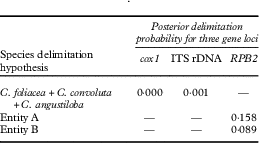
The results of the PTP analyses are listed in Table 4. The results of the ITS rDNA and cox1 analyses were congruent, both indicating that the C. foliacea complex (C. angustiloba, C. convoluta and C. foliacea) is one single species. However, this species has low support (Table 4). The RPB2 analysis resulted in two species, corresponding to the subclade called entity A and the remaining specimens (called entity B), with low support (Table 4).
Poisson Tree Processes (PTP) analyses. The values are posterior probabilities of species. The posterior probabilities for the outgroup species are not indicated. Highly supported species have a posterior probability >0·95. Entity A and B are putative species. Dashes indicate that this putative species was not delimited in this analysis

The results of the ABGD analysis of ITS rDNA dataset estimated only one group in the C. foliacea complex (prior maximal distance P=0·001).
The results of the BPP analyses are summarized in Table 5. The BPP1–5 analyses identified the combination C. foliacea plus C. convoluta as a single species with high probability. These analyses also determined that C. angustiloba is a different species from C. foliacea and C. convoluta. However, the BPP6–10 analyses (with different assignment criterion) considered the entity A and B as putative species, while A+B had low support.
Summary of results from species validation analyses using BPP under different species assignment and Gamma priors. The values are posterior probabilities (0·0–1·0) of putative species. Highly supported species have a posterior probability >0·95. The posterior probabilities for the outgroup species are not indicated. Dashes indicate that the species was not delimited in the best model

Gamma distribution for prior for each analysis: BPP1 & BPP6 ϴ~G(1,10), τ G~ (1,10); BPP2 & BPP7 ϴ~G(2,200), τ G~ (2,200); BPP3 & BPP8 ϴ~G(1,10), τ G~ (2,2000); BPP4 & BPP9 ϴ~G(2,2000), τ G~ (1,10); BPP5 & BPP10 ϴ~G(2,1000), τ G~ (2,2000).
The Bayes factor results are provided in Table 6. The species model that considers only one species in the C. foliacea complex was better than the other models, and the Bayes factor supported this model. The Bayes factor values based on the complete dataset were lower than those based on the dataset with at least two loci.
Comparisons of the different species delimitation models using Bayes factor (BF=2×(Model 1−Model 2)). The Bayes factor was computed to compare the current taxonomy, Model 1, with Models 2 and 3 and comparing Models 2 and 3. The first values of marginal likelihood correspond to the analyses based on the combined dataset with at least two loci and the second values correspond to the analyses based on the complete dataset

Discussion
In this study, molecular data were used in order to establish whether the species traditionally included in the Cladonia foliacea complex are independent lineages. This complex was previously addressed by Pino-Bodas et al. (Reference Pino-Bodas, Martin and Burgaz2010), who found no evidence of C. foliacea and C. convoluta being independent species. The present work focuses on a recently described species of this group, C. angustiloba (Ahti & Aptroot Reference Ahti and Aptroot2009). Few populations are known for this species, most of them in the Macaronesian region (Azores and Madeira). Though it is relatively easy to distinguish this species morphologically from the other two that form the C. foliacea complex, the characters separating them are quantitative rather than qualitative (length of the squamules, width and depth of the incisions). Since similar characters were used as diagnostic characters to separate C. foliacea from C. convoluta, the C. angustiloba case could be similar to that of C. convoluta (Pino-Bodas et al. Reference Pino-Bodas, Martin and Burgaz2010). The results did not support the traditional species as independent lineages. The data did not show genetic isolation between the traditional species; F st values were close to zero in most of the comparisons, they shared polymorphisms in several loci and fixed differences between species were not found (Table 2).
Discovery analyses did not separate the traditionally accepted species. However, their results are not totally congruent regarding the number of species and their limits. Frequently, different methods of species delimitation hold different delimitation hypotheses, often determining different numbers of species (Satler et al. Reference Satler, Carstens and Hedin2013; Singh et al. Reference Singh, Dal Grande, Divakar, Otte, Leavitt, Szczepanska and Lumbsch2015; Wei et al. Reference Wei, McCune, Lumbsch, Li, Leavitt, Yamamoto and Wei2016; Garrido-Benavent et al. Reference Garrido-Benavent, Pérez-Ortega and de los Ríos2017). It is generally assumed that GMYC overestimates the species diversity and that its results are greatly influenced by the sampling (Satler et al. Reference Satler, Carstens and Hedin2013; Hamilton et al. Reference Hamilton, Hendrixson, Brewer and Bond2014). Our GMYC analyses generated an unlikely number of entities in most cases (Table 3), though a low number of species was sometimes obtained (1 or 2). A single species was delimited by several analyses (GMYC, PTP and ABGD, Tables 3 & 4), while the GMYC single threshold analyses based on the combined matrix and RPB2 were congruent with the PTP analyses based on RPB2 and delimited two species. One of these species corresponded to the subclade detected in the phylogenetic analyses and the other comprised the remaining specimens. The species validation tests based on BPP analyses do not rectify the problem since the results were different depending on the assignment criterion used (Table 5). Cladonia angustiloba was supported in some of the BPP analyses; however, this species was not found by any of the discovery methods. Though many authors have considered BPP as a robust method for species delimitation (Zhang et al. Reference Zhang, Zhang, Zhu and Yang2011; Brown et al. Reference Brown, Tejangkura, El Mouden, Ait Baamrane and Znari2012; Giarla et al. Reference Giarla, Voss and Jansa2014), especially in those species complexes where speciation is recent (Leavitt et al. Reference Leavitt, Divakar, Crespo and Lumbsch2016), the usefulness of this method for delimiting species has been questioned (Sukumaran & Knowles Reference Sukumaran and Knowles2017). These authors adduce that BPP overestimates the number of species since it is not able to distinguish between population structure and barriers among species. Owing to the incongruities of the other methods, we consider that BPP could be detecting the existence of low levels of gene flow among populations, which could be expected because of the great distance between the Azores populations and those on the European continent. This could be the reason why C. angustiloba appears to be a different species using this method while it is not separated by the rest of the analyses. Another issue relative to BPP is the consistency of the results depending on the priors used. In the approach recommended by Leaché & Fujita (Reference Leaché and Fujita2010), we carried out the analyses with different priors and conclude that they slightly affect the probability of delimiting multiple species (Table 5). The delimitation results were similar, except that we obtained small differences in the probability of every species delimited. Nevertheless, it seems that the assignment of individuals to species is what most affects the results. The best values of Bayes factor in all the analyses were obtained with the hypothesis that considers only one species in the complex (Model 3). The Bayes factor indicated that both Models 2 (two species, entity A, entity B) and 3 (one species) are better than the current taxonomy. However, the Bayes factor slightly favoured the model with a single species in the complex (Model 3). The missing data did not affect the final result but the Bayes factor value was much lower in the analyses based on the complete dataset than that based on at least two loci. This result contrasts with those of Dembo et al. (Reference Dembo, Matzke, Mooers and Collard2015) who found that missing data lead to low Bayes factor values and could not differentiate between the hypotheses.
The species delimitation hypothesis that circumscribes two species is not supported morphologically. Specimens with different squamule sizes are grouped together in both putative species. The morphological studies carried out by Pino-Bodas et al. (Reference Pino-Bodas, Martin and Burgaz2010), based on measures of length, width and thickness of squamules and conidia length, indicated that the two subclades obtained using RPB2 phylogeny were morphologically very variable. The two putative species were not associated with different types of substratum (Fig. 1). Though cryptic species are very common in lichens (Crespo & Pérez-Ortega Reference Crespo and Pérez-Ortega2009; Crespo & Lumbsch Reference Crespo and Lumbsch2010; Molina et al. Reference Molina, Del-Prado, Divakar, Sánchez-Mata and Crespo2011; Parnmen et al. Reference Parnmen, Rangsiruji, Mongkolsuk, Boonpragob, Nutakki and Lumbsch2012; Singh et al. Reference Singh, Dal Grande, Divakar, Otte, Leavitt, Szczepanska and Lumbsch2015), we do not consider this to be the case in the C. foliacea complex. The hypothesis of a single species was the one favoured by PTP analyses based on ITS rDNA and cox1, the GMYC single threshold model of ITS rDNA and cox1, the ABGD method, and the Bayes factor. In the absence of further evidence, we consider the hypothesis that circumscribes a single species in this complex as the most probable one and therefore C. angustiloba and C. foliacea are the same species. This conclusion is also based on the widely known observation that a number of species within this genus are morphologically highly variable (Ahti Reference Ahti2000). Island populations often suffer morphological divergence from the continental ones (Cody Reference Cody2006; Lecocq et al. Reference Lecocq, Vereecken, Michez, Dellicour, Lhomme, Valterová, Rasplus and Rasmont2013) because they are subjected to different environmental conditions. The same occurs in other Macaronesian Cladonia species, where taxonomic differences were attributed to continental and island populations. Nevertheless, it has been recently demonstrated that in some cases no genetic differences exist between continental and island populations; some ‘endemic’ Macaronesian Cladonia taxa have been synonymized with widespread continental species, such as C. azorica, C. macaronesica and C. rangiformis var. gracillima (Pino-Bodas et al. Reference Pino-Bodas, Burgaz, Laguna, Stenroos, Ahti and Martín2015b , Reference Pino-Bodas, Pérez-Várgas, Stenroos, Ahti and Burgaz2016). Differences in squamule morphology that characterize C. angustiloba are a mere adaptation to local conditions.
A much overlooked feature causing variation in the morphology of the C. foliacea complex is the accumulation of calcium oxalate in the thallus. The importance of this phenomenon to lichen morphology and taxonomy was noted by Schade in several papers (e.g. Schade Reference Schade1964, Reference Schade1965, Reference Schade1966, 1967 Reference Schadea , Reference Schadeb ). He especially studied C. subrangiformis Sandst., which he regarded as C. furcata which has an altered, swollen morphology due to high accumulation of calcium oxalate in calcareous habitats (Schade Reference Schade1966). In fact, our earlier molecular study of this group was consistent with Schade in that C. subrangiformis should be united with C. furcata (Pino-Bodas et al. 2015 Reference Pino-Bodas, Burgaz, Martín, Ahti, Stenroos, Wedin and Lumbscha ). Schade listed C. foliacea ‘var. convoluta’, C. pyxidata ‘var. pocillum’, C. rangiformis, and C. ‘symphicarpia’ (= C. symphycarpa) as well as C. coniocraea among some other lichens concentrating calcium oxalate in large amounts (e.g. Schade 1967 Reference Schadeb ). The status of C. pocillum has been questioned by molecular studies (Kotelko & Piercey-Normore Reference Kotelko and Piercey-Normore2010), although many authors still accept that taxon. The status of C. macroceras should likewise be re-examined in light of its apparent accumulation of calcium oxalate in certain regions (cf. Fontaine et al. Reference Fontaine, Ahti and Piercey-Normore2010). Similarly, the taxonomic status of the calcicolous (calcium oxalate-containing) segregates of Vulpicida (Cetraria) juniperinus, viz. V. tilesii and V. tubulosus, recognized by the monographer Mattsson (Mattsson & Lai Reference Mattsson and Lai1993), were doubted by Schade (Reference Schade1966) and recently united with V. juniperinus on the basis of molecular analyses (Saag et al. Reference Saag, Mark, Saag and Randlane2014).
Thus, the Cladonia foliacea complex may be the result of the influence of the calcareous nature of its habitat on its morphology, whereby thalli of C. convoluta are longer and wider than those found in acidic or slightly calcareous habitats (‘C. angustiloba’, ‘C. foliacea s. str.’). However, even in the Nordic countries and Siberia, C. foliacea (with small squamules) is normally calciphilous, avoiding widespread acidic habitats.
The species delimitation studies should be included with the species names and the formal descriptions of the newly delimited taxa. Therefore, C. angustiloba and C. convoluta are here officially synonymized with C. foliacea.
Taxonomy and Nomenclature
All the important names at species level of the Cladonia foliacea complex are summarized below with indications of types as far as they are known. Many entries include additions or corrections to other sources, such as the Index Fungorum. Numerous authors have used varietal or subspecific epithets for the conspicuous morphs of this group. Schade (e.g. 1965) applied expressions such as ‘m. (= modification) subrangiformis’. Another informal expression is ‘morph convoluta’, if one wishes to indicate a certain commonly recognized and obvious environmental modification. A DNA extraction from an isoepitype of C. foliacea (Leighton, Lich. Brit. Exs. No. 15, H) was carried out but the amplifications failed (Pino-Bodas et al. Reference Pino-Bodas, Martin and Burgaz2010). Specimens similar to the types and collected close to the type locality were included in the analyses (C. foliacea, Scotland, MACB 95602; C. convoluta, France, Hérault, H; C. angustiloba, Azores, Pico Island, Candelaria, CL798, H).
Cladonia foliacea (Huds.) Willd.
Fl. Berol. Prodr.: 363 (1787).
Basionym. Lichen foliaceus Huds., Fl. Angl. 457 (Jan–Jun 1762); type: Icon in Dillenius, Hist. Musc., tab. 14, fig., 12A (1742), lectotype designated by Ahti & Stenroos (Reference Ahti and Stenroos2013): 91; England, Salop (Shropshire), Haughmond Hill, W. A. Leighton in Leighton, Lich. Brit. Exs. No. 15 (BM—epitype, designated by Ahti & Stenroos Reference Ahti and Stenroos2013: 91; H, UPS—isoepitypes).
= Lichen sterilis Gouan, Illustr. 82 (1773); type: France, A. Gouan (PC—syntype; H-ACH 1734, 1735—possible syntypes).
= Lichen substerilis Gouan, Illustr. 82 (1773); type: France (not designated, but original material seen by Dufour Reference Dufour1821).
= Cladonia alcicornis (Lightf.) Fr., Lich. Exs. Suec. No. 210 (1826).
Basionym. Lichen alcicornis Lightf., Fl. Scot. 2: 872 (20–23 Sep. 1777); type: Scotland (not designated).
= Lichen ambiguus Latourr., Chlor. Lugd. 35 (1785); type: France, M. Latourrette (PC—lectotype designated here).
= Lichen nivalis Vill., Hist. Pl. Dauphin. 3(2): 935 (12 Sep.–22 Oct. 1789), nom. illeg. (later homonym, non Lichen nivalis L. 1753); type: France (not seen; cf. Vainio Reference Vainio1894: 386).
= Cladonia convoluta (Lam.) Anders, Strauch-Blattflecht. Nordböhm.: 29 (1906).
Basionym. Lichen convolutus Lam., Fl. Franç. 1(3): 84 (21 Mar. 1779 ‘1798’); type: France, Paris, Bois de Boulogne, J. Deslongchamps s. n. (P-LA—neotype designated here).
Cladonia foliacea subsp. convoluta (Lam.) Suza, Lich. Bohemoslovakiae Exs. No. 225 (1933).
Cladonia foliacea var. convoluta (Lam.) Vain. Acta Soc. Fauna Fl. Fenn. 10: 394 (Dec. 1894).
= Cladonia endiviifolia (Dicks.) Fr., Lich. Eur. Ref. 212 (Jun–Jul 1831).
Basionym. Lichen endiviifolius Dicks., Fasc. Pl. Crypt. Brit. 3: 17 (Sep. 1793), ‘endiviaefolius’; type: England (not seen).
= Lichen crocatus Dicks., Hortus Siccus Brit. 4: No. 24 (1795), nom. illeg. (later homonym, non Lichen crocatus L. 1771); type: England, J. Dickson, Hortus Siccus Brit. No. 24 (BM, not seen).
= Cenomyce damicornis Schleich., Cat. Pl. Helv. (ed. 2): 32 (1807), ‘damaecornis’, nom. nudum.
= Cenomyce damicornis Ach., Lichenogr. Universalis 530 (Apr–Mai 1810), ‘damaecornis’, nom. illeg, (superfl. for Lichen convolutus Lam. 1779).
= Cladonia damicornis Buch, Phys. Beschr. Canar. Ins. 199 (1828) (‘1825’), nom. illeg. superfl. (based on Cenomyce damicornis Ach., Lichenogr. Universalis 530 (Apr–Mai 1810), nom. illeg. superfl. for Lichen convolutus Lam. 1779).
= Lichen endiviolus Brot., Fl. Lusit. 2: 459 (10 Jul 1805) (‘1804’); type: Portugal (not designated).
= Cladonia vaillantii Dufour, Ann. Gén. Sci. Phys. 8(22): 52 (Apr. 1821), nom. illeg. superfl. for six species cited.
= Cladonia cornucopiae Spreng., Syst. Veg. 4: 272 (1827); type: not designated.
= Cladonia convoluta var. vagans Follmann, Philippia 2: 208 (1 Apr. 1975) (‘1974’); type: Spain, Teruel (‘Hispania, Aragonia’), Sierra de la Costera, near Fuentes Calientes, 1973, G. Follmann in Follmann, Lich. Exs. Casselenses, No. 145 (B—holotype; BCC, DUKE, H, LD, O, TNS, TUR, UPS—isotypes).
= Cladonia angustiloba Ahti & Aptroot, Biblioth. Lichenol. 99: 12 (2009); type: Azores, Pico, São João, 30 m, on coastal lava, 7-VII-2007, A. Aptroot 67832 (H—holotype; ABL—isotype).
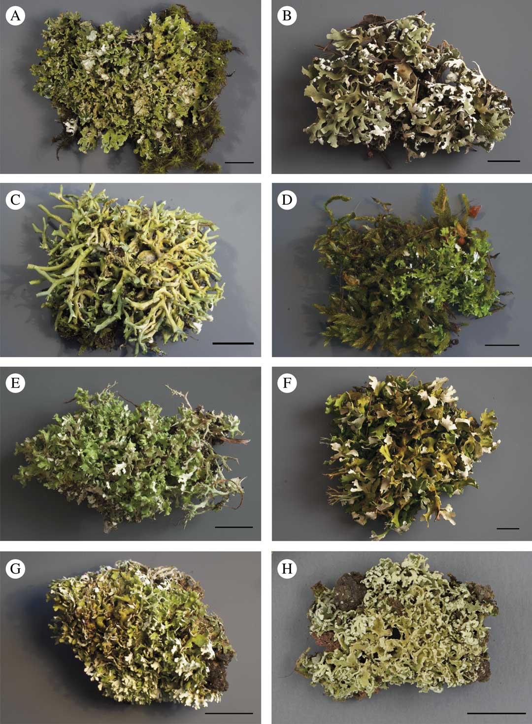
(Fig. 2)
Morphological variation of Cladonia foliacea. A, C & F, ‘morph convoluta’; B, D, E & G, ‘morph foliacea’; H, ‘morph angustiloba’. A, Cyprus, Nicosia, Kakopetria A. R. Burgaz s. n. (CL852); B, France, Var, Esterel Massif, A. R. Burgaz s. n. (CL840); C, France, Bouches-du-Rhône, Auriol, A. R Burgaz s. n. (CL850); D, Hungary, Pest, Szobi, Kemence, A. R. Burgaz s. n. (CL853); E, Cyprus, Nicosia, Pedoulas, A. R. Burgaz (CL851); F, Hungary, Veszprém, Királyszentistván, A. R. Burgaz s. n. (CL838); G, Greece, Macedonia-Tracia, Chalkidiki, A. R. Burgaz s. n. (CL839); H, Portugal, the Azores, Pico, Candelaria, road to Pocinho, R. Pino-Bodas (CL798). Scales=1 cm. In colour online.

Primary thallus persistent, dominant, squamulose, forming dense mats 3–10 cm diam. with ascending or prostrate squamules; squamules well developed, (0·5–)6·6–21·6(–38·0)×(0·3–)1·3–3·7(–6·3) mm (n=133); upper side yellowish green, smoothly corticate to maculate-verruculose; lower side pale yellow, arachnoid; margin irregularly lobate to deeply divided, with laciniate squamules, sometimes with black marginal hairs. Squamules (200–)318–548(–830) μm thick, cortex (37·5–)54·3–99·7(–166·7) μm, algal layer (10·0–)27·7–49·5(–77·5) μm, medulla (100·0–)201·5–415·0(–680·0) μm.
Podetia infrequent, (0·3–)3·3–11·0(–20·0) mm tall (n=51), (0·10–)0·75–2·00 (–3·00) mm thick, yellowish-green, single with closed scyphi. Surface of podetia corticate, smooth to verrucose; conidiomata on primary squamules, more rarely on the tip of the podetia, abundant, brown to black, (220–)260–530(–850) μm (n=22) tall, subglobose to pyriform, constricted at base, with hyaline slime; conidia falciform to straight, hyaline, (–5·0)5·7–(8·3(–11·0) μm long (n=182); hymenial discs brown, (1·0–)1·3–3·3(–5·0) mm wide; ascospores simple, hyaline, (6·0–)8·0–11·8(–18·0)×(2·0–)2·6–3·5(–4·0) μm (n=90).
Chemistry. Two chemotypes: 1) C−, K−, P+ orange to red, containing usnic acid (major), fumarprotocetraric acid (major) and protocetraric acid (minor); 2) C−, K−, P+ orange to red containing usnic acid (major), fumarprotocetraric acid (major), protocetraric acid (minor), psoromic acid (major), conpsoromic acid (minor). Chemotype 1 is the most common. In addition, it contains other minor satellites of fumarprotocetraric acid, such as confumarprotocetraric acid (Cph-2) (Geyer Reference Geyer1985; Huovinen et al. Reference Huovinen, Ahti and Stenroos1989) and occasionally zeorin (Burgaz & Ahti Reference Burgaz and Ahti2009; Ahti & Stenroos Reference Ahti and Stenroos2013). The ‘morph convoluta’ seems to contain higher concentrations of usnic acid and is therefore also more yellow (Geyer Reference Geyer1985).
Distribution. There are numerous local distribution maps of C. foliacea and C. convoluta (listed by Scholz Reference Scholz2007), and a world map of C. convoluta (Litterski & Ahti Reference Litterski and Ahti2004). In the herbaria we have noticed that the limit of C. foliacea and C. convoluta has been variously interpreted, but there are large areas where only one morph is present. When the map of the ‘morph convoluta’ cited by Litterski & Ahti (Reference Litterski and Ahti2004) is supplemented with the other morphs and new records, the range widens to southern Scandinavia, the Faroe Islands, and eastwards to Sakha Republic (Yakutia), Altay and Mongolia. In Africa the species extends to the Cape Verde Islands, Mauritania and Egypt. The species is known primarily from southern and central Europe, northern Africa, the Near East and western Siberia. Additions to the countries and provinces listed by Litterski & Ahti (Reference Litterski and Ahti2004) are Albania, Altay, Cape Verde, Denmark, the Faroe Islands, Finland, Ireland, the Netherlands, Latvia, Libya, Lithuania, Luxembourg, Mauritania, Mongolia, Norway, Sakha Republic, San Marino and Syria.
Selection of specimens examined. Albania: Korçë: Pogradec Udënisht, SH3 Piskutat-Pogradec, shore of Ohrid Lake, 40°58′55″N, 20°38′21″E, alt. 710 m, 22 iv 2017, A. R. Burgaz (MACB).—Armenia: Gegharkunik: Sevan, Sevanavank, 40°33′50″N, 45°00′48″E, alt. 1950 m, 22 vi 2015, A. R. Burgaz (MACB).—Bosnia and Herzegovina: Federation of Bosnia and Herzegovina: Herzegovina-Neretva Canton, Bijakoviči, Medjugorje, way up to the Hill of Apparitions, 33TYH188845, 200 m, karstic limestone, 26 iii 2010, A. R. Burgaz (MACB).—Cape Verde: São Antão: Lombo das Pedras, alt. 1350 m, 1987, B. Mies 490d (H).—Croatia: Dubrovnik–Neretva County: Zamaslina, Pelsejac Peninsula, 33TYH231456, alt. 20 m, 31 iii 2010, A. R. Burgaz (MACB).—Georgia: Shida Kartli-Kareli: Akhaltsikhe, Tsini-Giorgitsminda, 42°01′28″N, 43°54′04″E, 12 vii 1968, Ts. Inashvili (TBI).—Hungary: Bács-Kiskum: Fülöpháza, 46°52′13″N, 19°25′22″E, alt. 125 m, 25 v 2015, A. R. Burgaz (MACB).—Kazakhstan: Qaraghandy (Karaganda) Region: near Karkaraly (Karkaralinsk), alt. 800 m, 1963, H. Aasamaa (H).—Mongolia: East Khangay Mts: Övörkhangay aimak, Mt. Ust-Uul, alt. c. 200 m, 1978, L. G. Byazrov 6451 (H).—Portugal: Madeira: Montado dos Pecegueiros, Levada by Caldeirão Verde, alt. 900 m, 1975, A. Henssen 22526L (H).—Spain: Álava: Leza, Sierra de Cantabria, pto. de Herrera, 30TWN2714, alt. 905 m, 26 vii 2006, A. R. Burgaz (MACB). Jaén: Otiñar, Sierra de Jaén, Quiebrajano River, 30SVG3273, alt. 570 m, 4 iv 2009, A. R. Burgaz (MACB).
Additional specimens studied can be found in Table 1, Table 1 of Pino-Bodas et al. (Reference Pino-Bodas, Martin and Burgaz2010) and Burgaz (Reference Burgaz2015).
We (TA and SS) are grateful to Dr Volker Otte (Görlitz) for help with our study of A. Schade’s collections in Görlitz (GLM) and Dr Jaana Haapala, who helped us with photographs. RP-B was supported by the grant Juan de la Cierva-Incorporación 2015-23526. ARB acknowledges financial support by the project CGL2013-41839-P (Ministry of Economy & Competitiveness, Spain).