

How do economic crises impact trade policy? Scholars tend to oscillate between three alternate views. Some argue that crises sow the seeds of trade liberalization, while others posit a strong link between shocks and increased protectionism, and a third camp contends that there is no generalizable relationship between economic distress and policy adjustment.Footnote 1 The controversy is understandable given the significant variation in observed responses to hard times. For example, while South Korea responded to economic adversity by liberalizing its trade policies in the 1980s, Thailand reacted to its 1997 crisis with increased protection. Likewise, Mexico lowered its tariff barriers in the 1980s in response to a debt shock, while Chile raised them in response to a similar situation. Although the Great Depression immediately led to increased trade protection in most nations, the 2008 financial crisis did not cause similarly severe and widespread tariff hikes. These diverging responses have prompted many to argue that the relationship between economic crises and policy reform is both ‘theoretically indeterminate and empirically questionable’.Footnote 2
We develop a theoretical framework that provides a unified explanation for observed variation in trade policy following crises. Our approach builds on three key insights. First, we observe that the political maneuverings of distressed firms typically have ‘knock-on’ effects on the resources and strategies of other firms in the economy. Our model incorporates these ripple effects, thereby capturing the dynamics by which competing special interests jointly shape the policy-making process. Secondly, because the scarcity of resources is a defining characteristic of ‘politics in hard times’,Footnote 3 we notice that firms seeking to influence policy outcomes are much more likely to run out of lobbying resources during a crisis than otherwise. By focusing on the implications of shrinking budgets, our theoretical framework explicates how shocks to resources can impact the political strategies of firms and, in turn, precipitate policy reform. Thirdly, we show that particular features of shocks can erode profits and shape lobbying dynamics in distinct ways. For example, a sharp but short-lived shock might trigger different policy reverberations than a less severe yet sustained period of distress. Our modeling approach identifies, and conceptually distinguishes between, two core characteristics of crises: intensity and duration. We disentangle the mechanisms by which both features of shocks recalibrate political strategies and trigger policy revision.
With these simple theoretical innovations, we generate a framework to explain the trade policy responses to crises of varying severity and length. We find that tariff rates display an inverted-U shaped relationship in the intensity of shocks, initially rising in shock severity and then falling as the magnitude of the shock surpasses a critical threshold. The intuition for our argument is as follows: at any given time, the more acutely they are hit by economic shocks, the more vigorously industries lobby for trade protection – but only up to a point. When shocks are inordinately large, the tariff levels required to sustain profitability in the suffering industry become so high that other industries seeking liberalization have greater incentives to counter-lobby, which ratchets up the lobbying costs required to secure protection. The relationship between the intensity of an industry-level shock and the tariff protection afforded to that industry is therefore characterized by an inverted-U shape.
We find a similar ‘up-down’ pattern in the relationship between protectionism and the duration of crises. The logic tying the length of shocks to trade protection is related but distinct. Protection initially increases when industries lobby heavily for assistance, but then decreases as industries run low on resources to expend on lobbying and as firms in other industries mobilize to counter-lobby and demand liberalization. Importantly, we demonstrate that these competitive changes in tariff policy stem directly from industries’ political strategies during the crisis itself, and do not reflect policy adjustments to shocks abating over time. A focus on the mechanisms by which crises erode industries’ resource endowments, which in turn influences lobbying and counter-lobbying dynamics, leads us to predict that economic distress first generates autarkic pressures but then leads to freer trade when shocks to profitability persist.
Our theory helps explain a wide swath of historical and contemporary cases, from the introduction and repeal of the Corn Laws to tariff adjustments during the 1980s debt crises in Latin America to policy reconfigurations in the midst of the Great Depression. The regulatory dynamics that we highlight build on insights developed in the vast literature on the effects of economic shocks. Yet extant studies have largely focused either on increased protection or increased liberalization, and tend to explain policy transformations by considering how governments – rather than industries – respond to economic stresses. By studying the strategic interactions between political agents and different types of firms and industries in the economy, we are able to explain both the protectionist and liberalizing pressures of crises within a unified framework. Our theory relies on minimal assumptions, draws on dynamics that resonate closely with real-world examples, and offers a generalizable account of the relationship between shocks and policy adjustment.
In the remainder of the article, we flesh out these predictions and present evidence to support our theory. The next section situates our argument in the existing literature. We then develop our formal model, which allows us to generate specific predictions about the effect of crisis intensity and duration on trade policies. We include illustrative examples of countries that were struck by international crises to highlight the mechanisms by which economic shocks change lobbying patterns and influence policy changes. Finally, we conduct both a sub-national, industry-level empirical study, as well as a cross-national, time-series analysis and find strong support for our predicted relationships.
Links Between Economic Crises And Trade Policy
Considerable controversy surrounds the impact of economic crises on trade protection. Traditionally, scholars have postulated that there is a positive relationship between these variables,Footnote 4 citing factors such as increased pressure to safeguard domestic industries and interest groups,Footnote 5 the political difficulty of implementing liberal policies during economic downturns while politicians are less popularFootnote 6 and a regime’s desire to tighten control over the economy.Footnote 7 This body of work also posits that domestic political coalitions are important determinants of protection in times of crisis,Footnote 8 as the incentives to lobby for protection often depend on membership in these groups.Footnote 9 Many comparative studies, in turn, shed light on how crises reorient domestic coalition preferences in favor of protectionism.Footnote 10
By contrast, a second body of scholarship contends that economic shocks more often serve as catalysts for trade liberalization.Footnote 11 According to these accounts, crises break apart ossified special interest coalitions and provide politicians with the power to enact previously unpopular economic reforms, including tariff deregulation.Footnote 12 Some scholars posit a conditional link between downturns and policy change; for example, CorralesFootnote 13 argues that governments liberalize following crises in proportion to their capacity to sustain reforms. Other scholars speculate that crises might in fact be necessary for liberalization,Footnote 14 as they are needed to discredit current policies and empower reform-oriented interests in the political arena.Footnote 15
A third body of scholarship argues that the relationship between crises and trade policy is – all things considered – ambiguous. For example, WeylandFootnote 16 observes that responses to economic shocks can vacillate between protection and liberalization, depending on whether particular actors view themselves to have gained or lost from the downturn. Policy change following crises might depend on the contemporary macroeconomic context,Footnote 17 domestic support resulting from particular sectoral and factor allocations,Footnote 18 or specific domestic institutions.Footnote 19 These studies illustrate how economic crises can precipitate a wide variety of political responses, and suggest that no systematic theory can explain when and how crises result in protection versus liberalization.Footnote 20
The purpose of our article is to develop and test such a theory. We do so by incorporating the impact of crises on industry-level resources for lobbying and counter-lobbying. Our theoretical framework builds on the seminal Grossman and Helpman (G-H) model of special interests,Footnote 21 in which industries provide political contributions to a government that maximizes a weighted welfare function balanced between lobbying dollars and social well-being.Footnote 22 While subsequent work has modified the G-H framework in various ways, these formal accounts consider neither the role of economic crises in shaping tariff outcomes – the central focus of our article – nor the mechanisms by which political competition between firms drives policy-making dynamics during downturns.Footnote 23
To explicate the channels through which economic shocks impact different sectors in the economy, we introduce two simple yet powerful innovations to the G-H framework. Our first departure is the observation that opposition from downstream or complementary industries plays an important role in trade policy making. Historical accounts from a wide range of cases indicate that greater protection for one industry time and again sparks counter-lobbying in another, particularly downstream manufacturers or those engaged in complementary economic activities. For example, the US sugar and sweetener industry regularly lobbies for, and secures, protection against cheaper foreign imports.Footnote 24 But higher sugar tariffs simultaneously harm domestic confectionery manufacturers, which face steeper costs in the production process.Footnote 25 It is no surprise, then, that candy makers deploy significant resources to lobby US representatives against sugar tariffs.Footnote 26
Scholars have examined counter-lobbying as a potential counterweight to protectionist interests, finding indirect evidence of counter-lobbying activities both when foreign lobbies are present and when the effects of domestic counter-lobbying are analyzed cross-nationally.Footnote 27 Additionally, by explicating the effects of counter-lobbying on trade protection, recent work in ‘new new’ trade theory has provided new insights into our understanding of trade policy making. For instance, KimFootnote 28 argues that high product differentiation reduces counter-lobbying pressures, in turn lowering tariffs; OsgoodFootnote 29 similarly points out that industries with highly differentiated products can have different preferences over trade policy. To date, however, this work has largely focused on understanding trade politics in ‘normal’ times, and has not been extended to periods of economic distress. More broadly, despite its far-ranging impact, competition between various sectoral lobbies remains both ‘highly circumscribed’ in general models of trade policy making,Footnote 30 and entirely absent in models that study the relationship between crises and trade policy responses.
Our second innovation is to note that every firm – and, consequently, every industry – faces a budget constraint that limits lobbying. The G-H model does not consider policy dynamics when firms seek protection, but simply do not have lobbying resources to influence change. This omission is understandable, as the G-H model does not attempt to explain special interest politics during crises. When it is ‘business as usual’, firms typically have access to vast financial resources that can be deployed toward lobbying. However, it is precisely during periods of widespread economic distress – when the financial system cuts back on lending, and when sources of credit evaporate for distressed firms – that struggling industries are most likely to face budgetary limits on lobbying activities.
We posit that the threat of a binding budget constraint can systematically alter the dynamics of crisis politics. To examine how shrinking budgets impact industries’ political strategies, we start by borrowing insights from a separate literature that studies how aging firms collapse.Footnote 31 This body of work makes the intuitive claim that dwindling resources can push senescent industries out of business. We then study how counter-lobbying pressures mediate the policy-making process in the presence of economic shocks of varying length and severity.Footnote 32 Incorporating the notion of a binding budget constraint into our theoretical framework of lobbying and counter-lobbying allows us to generate new and previously untested predictions about the link – in particular, the curvilinear, ‘up-down’ relationship – between economic shocks and policy revision. We show that accounting for this interplay is critical for properly explaining how special interest competition affects trade policy outcomes in the wake of crises.Footnote 33
A Model Of Trade Policy Responses To Economic Shocks
Consider a country with two industries, A and B, as well as a government, G. The country is integrated into world markets, yet may also engage in trade protection in order to safeguard the profitability of domestic industries. We focus our analysis on the impact of economic shocks on trade protection for a good produced by industry A. Given a world price of w for this good, the government can impose an additional linear tariff rate of
 $$\tau $$
such that A’s domestic price becomes
 $$p=w{\plus}\tau $$
. Further, A’s profits (π
A (p)) are concave in p.Footnote
34
Following the trade politics literature, we assume that A offers the government a schedule of lobbying payments
 $$(l_{A} _{{}} (\tau ))$$
for each potential
$$\tau $$
, which the government then considers when selecting a particular
$$\tau $$
.Footnote
35
Industry B uses the good produced by A as an intermediate input, such that B’s profits (π B (p)) are indirectly a function of A’s domestic price. For instance, if industry A represents steel manufacturers, B could be any industry that uses steel as an input, such as the construction or automobile industry. Although a jump in the price of steel increases profits for the former, such a change reduces profits for the latter because it raises the cost of intermediate inputs for these downstream producers.Footnote 36 As is standard, we assume that when the value of p is lower, B faces a larger marginal loss from an increase in p. For example, the losses associated with a price increase from $1 to $2 are larger than those associated with an increase from $100 to $101.Footnote 37
While many industries are impacted by input costs in this manner, not every industry is affected by this consideration to the same degree.Footnote
38
In order to investigate the effects of the varying sensitivity of downstream industries to changes in their own industry prices, we introduce an additional parameter σ
i
which captures the sensitivity of profits in a given industry to changes in the price of good A. There are a number of natural interpretations of σ
i
: as π
B
(·) captures the amount by which profits in B fall for an increase in the price of A, this corresponds easily to costs that arise from the procurement of intermediate goods. In this case, σ
B
represents the degree to which these costs directly detract from B’s profits. For firms with few downstream consumers, we might imagine that this sensitivity parameter would be relatively low, whereas for firms that produce essentially no finished products, the sensitivity of downstream manufacturers to prices in the initial good is likely to be high. This sensitivity of downstream producers is likely to affect their preference for counter-lobbying against trade protection for industry A. Intuitively, in what follows we set σ
A
= 1,Footnote
39
while allowing the sensitivity of downstream producers to vary such that
 $\sigma _{B} =\sigma \in {\Bbb R}_{{\plus}} .$
Following previous examinations of counter-lobbying, if A gains tariff protection, B may then lobby the government to reduce the tariff on A’s good, denoted l
B
(
$$\tau $$
).Footnote
40
As is the case in Mitra’sFootnote
41
work, industries incur a fixed organizational cost to participate in lobbying activity, denoted κ
i
, where
 $i\in \left\{ {A,\,B} \right\}$
. For simplicity, we normalize κ
A
to zero, though our main comparative statics hold when we simply bound κ
A
at
 $\bar{\kappa }_{A} $
, which is the cost beyond which A never lobbies for protection. The industries’ indirect utility functions are therefore:
 $$u_{i} (\tau )\left\{ {\matrix{ {\sigma _{i} \pi _{i} (w{\plus}\tau ){\minus}\kappa _{i} {\minus}l_{i} (\tau )} & {if\,i\,lobbies} \cr {\sigma _{i} \pi _{i} (w{\plus}\tau )} & {otherwise.} \cr } } \right.$$
Finally, we assume that the government cares both about overall societal welfare and the lobbying resources it receives from industry i. Given a social welfare function of W (
$$\tau $$
), as well as a ‘benevolence’ parameter β that captures the degree to which the government favors welfare versus contributions,Footnote
42
the government’s utility function is:
 $$\Gamma (\tau )=\beta W(\tau ){\plus}(1{\minus}\beta )\mathop{\sum}\limits_i {l_{i} (\tau )} .$$
Social welfare is linear in
$$\tau $$
, such that
 $W(\tau )=\omega {\minus}\gamma \tau $
, where γ represents the marginal welfare loss of increasing the tariff, and ω is an intercept. γ captures many factors that influence
$$\tau $$
’s cost to society including the state’s reliance on trade, the importance of citizens’ consumption of the good, and the strength of domestic groups such as labor movements or consumer protection agencies.Footnote
43
However, industries may be able to compensate the government for these detrimental effects of tariff protection by lobbying. The game comprises the following stages:
1. Nature draws a world price
 $w\,\sim\,F(w).$
2. A selects an optimal tariff
$\tau _{A}^{{\asterisk}} \in {\Bbb R}_{{\plus}} .$
3. A selects a lobbying schedule
$l_{A} (\tau )\in {\Bbb R}_{{\plus}} .$
4. Observing these choices, B selects an optimal tariff
$\tau _{B}^{{\asterisk}} \in {\Bbb R}_{{\plus}} .$
5. B selects a lobbying schedule
$l_{B} (\tau )\in {\Bbb R}_{{\plus}} .$
6. Observing A and B’s lobbying schedules, the government selects the tariff, and pay-offs accrue.


We focus on sub-game perfect Nash equilibria, and solve by backwards induction. While the Appendix presents the full derivation of the equilibria, the next section fleshes out the key intuitions of the model. In so doing, we explicate the mechanisms by which economic crises impact competing industries’ political strategies and derive clear predictions about trade policy responses to shocks of varying intensity and duration.
Trade Protection and Shock Severity
To model the dynamics of trade policy making following economic shocks, we follow the G-H framework by examining how changes in domestic prices affect industries’ profits.Footnote 44 In particular, we represent these shocks as drops in the world price of the good produced by A. This creates downward pressure on the domestic price and, in turn, erodes A’s profits, which may lead A to lobby for trade protection. While downturns can arise from a variety of sources, as our qualitative and quantitative empirical evidence will subsequently illustrate, we focus here on shocks to w to fix ideas. This set-up yields the following prediction:
Proposition 1: Tariffs increase in crisis intensity initially, but decrease in crisis intensity beyond a specific threshold.
Proof. See Appendix .
The intuition for this proposition starts with the observation that the equilibrium tariff rate can be characterized by the size of the shock to w. Absent counter-lobbying pressure from B, A lobbies until the marginal costs of compensating the government for losses from trade protection equal A’s marginal profit gains, which occurs at price
 $\hat{p}$
.Footnote
45
When the price is above
$\hat{p}$
, the social welfare losses exceed A’s profitability gains, such that A does not lobby and no tariff is applied in equilibrium.
When the price falls below
$\hat{p}$
, A can potentially increase its profitability by lobbying for protection. Yet whether it does so depends on whether B counter-lobbies. Since B must pay an organizational cost to counter-lobby, doing so is not optimal when the tariff is small. In this case, A receives its ideal tariff rate, securing a domestic price of
$\hat{p}$
. As the shock’s intensity increases (that is, as w falls), equilibrium tariff levels rise. Thus, as long as shocks are not too large, higher tariff rate increases occur in industries facing more intense shocks, which is seen from an examination of A’s ideal tariff, or
 $$\tau _{A}^{{\asterisk}} =\hat p} {\minus}w.$$
However, because the social welfare distortions from A’s optimal tariff grow as the tariff increases, B’s counter-lobbying eventually becomes profitable. We denote by
 $\hat{w}$
the value of w where B is indifferent between counter-lobbying and not, such that
 $$\sigma \pi _{B} (\hat{w}){\minus}\kappa _{B} =\sigma \pi _{B} (\hat{p}).$$
When
 $w\geq \hat{w}$
, A continues to secure
 $\tau _{A}^{{\asterisk}} $
without facing any counter-lobby pressure from B; when
 $w\lt \hat{w}$
, B finds it profitable to enter the counter-lobbying market if A lobbies for
$\tau _{A}^{{\asterisk}} $
. B’s counter-lobbying threat leads A to seek a compromise tariff that allows it to retain some protection but does not incite a costly counter-lobbying battle with B.Footnote
46
A thus selects the tariff that makes B indifferent between counter-lobbying and not doing so, denoted
 $\tilde{\tau }$
, which satisfies
 $$\sigma \pi _{B} (w){\minus}\sigma \pi _{B} (w{\plus}\tilde{\tau })=\kappa _{B} .$$
Since A’s cost of obtaining a given tariff increases as w falls,
$\tilde{\tau }$
shrinks as w declines.Footnote
47
In other words, beyond the threshold
$\hat{w}$
, an increase in crisis intensity leads to a decrease in the equilibrium tariff. Combining this result with the discussion above, the tariff first increases in shock intensity up to the cut-point characterized by Equation 4, but then decreases in shock intensity thereafter.
Importantly, however, the model generates additional testable implications regarding how equilibrium tariffs are affected by the sensitivity of downstream industries (σ). As proven in the Appendix, the steepness of our inverted U is affected by changes in the sensitivity of industry B to changes in the price of good A: as sensitivity increases, the parameter space over which tariffs rise with crisis intensity is compressed. This has the effect of increasing the inflection point at which tariffs switch from rising to falling in crisis intensity, meaning that our inverted-U shape should be more pronounced. In addition, once the world price has dropped beyond this inflection point (such that equilibrium tariffs grow smaller as intensity increases), greater sensitivity in industry B accelerates the rate at which equilibrium tariffs fall. Taken together, these two effects of greater σ suggest that, when downstream industries are more sensitive to price changes in A, our inverted-U shape peaks sooner and drops more steeply. While it is difficult to quantify this sensitivity in the real world, it should vary systematically for two types of industries: those that produce intermediate goods, and those that produce final goods.
Trade Protection and Shock Duration
We now turn to the relationship between crises and trade policy over time, which requires the addition of two features to the model. First, we extend the model to two periods, allowing us to analyze temporal changes in equilibrium tariff levels. Secondly, we impose a budget constraint on industry A, stipulating that A must receive a non-negative pay-off in every period. Because industries often have access to ‘war chests’ to continue operations during hard times, we also add a source of (initially exogenous) resources that A uses to lobby, denoted ρ i. We conceptualize these resources as residual profits from past play, but they may more generally capture any initial financial advantages enjoyed by a particular industry at the outset of a crisis, such as access to loans or additional leverage due to the size of the industry.Footnote 48 Formally, we now specify A’s per-period pay-off as:
 $$u_{{At}} (\tau _{t} )=\pi _{A} (w{\plus}\tau _{t} ){\plus}\rho _{t} {\minus}l_{A} (\tau _{t} ).$$
Imposing a budget constraint requires this expression to be non-negative, such that industry profits at a given level of protection, plus any additional financial resources, are sufficient to cover the costs of lobbying the government for this protection.Footnote 49 When this budget constraint does not hold, A leaves the market, securing a reservation pay-off of zero thereafter. Finally, while outside resources are determined exogenously in period one, in subsequent rounds they are set as residual profits from previous play. Therefore, although A may have access to extra resources at the beginning of a crisis, it cannot rely indefinitely on outside finances.Footnote 50 Extra resources in the second round comprise A’s remaining funds, orFootnote 51
 $$\rho _{{t{\plus}1}} =\pi _{A} (w{\plus}\tau _{t} ){\plus}\rho _{t} {\minus}l_{A} (\tau _{t} ).$$
We focus here on Markovian Perfect Equilibria, with ρ t and w as the two main state-relevant variables. To isolate the effect of crisis duration, we hold the intensity of the crisis constant; since we model economic crises as a shock to w, we consider the case in which the shock drawn in the first period persists into the second period.Footnote 52 This allows us to identify dynamics of policy competition that take place entirely within the confines of the economic crisis. Policy reverberations thus flow directly from the political maneuverings of industries as they respond to hard times and are not driven by shocks simply waning over time – a widely held alternate assumption in scholarly and policy writings. Using this set-up, we find the following:
Proposition 2: Tariffs initially increase during a crisis, but subsequently decrease in crisis duration.
Proof. See Appendix .
Though A’s ideal tariff considerations are largely identical to those of the one-period game discussed above, imposing a budget constraint introduces an additional complication to A’s equilibrium strategy: for A to favor a higher tariff, A must be able to afford it. If A can pay for the lobbying costs associated with setting its ideal tariff level using only its current-period profits (that is, without recourse to ρ t), then the outcome of the stage game is identical to that of the one-shot game described above. Yet if A can only afford its ideal tariff by dipping into its war chest, then an additional temporal dynamic comes into play.
To illustrate, we consider the effect of a shock such that
 $\hat{w}\leq w\lt \hat{p}$
, where A wishes to lobby for its ideal tariff as given in Equation 3, which is not large enough to incite counter-lobbying. A’s profit-maximizing tariff equates the marginal profitability with the marginal welfare loss associated with its imposition. Yet in industries with low profitability, or when the welfare losses from trade protection are particularly high, A may not be able to afford this tariff using existing profits.Footnote
53
In such cases, A can still secure its preferred tariff if its additional resources cover the difference.Footnote
54
The tariff therefore rises in reaction to falling world prices in the first period, as A is able to secure its ideal level of protection.
Whether this strategy remains feasible in the second period depends on A’s remaining resources, ρ
t+1, because dipping into the war chest to help fund its lobbying activities in the first period decreases the outside resources available in subsequent periods.Footnote
55
The equilibrium tariff may thus differ in the second round. Specifically, if the budget constraint binds when A lobbies for
$\tau _{A}^{{\asterisk}} $
in the second period, the equilibrium tariff does not change. Yet if ρ
t+1 has been reduced to the point that it no longer covers the difference between
 $\pi _{A} (\tau _{A}^{{\asterisk}} )$
and
 $l_{A} (\tau _{A}^{{\asterisk}} )$
, A is forced out of the market and the government reverts to free trade. We therefore find that equilibrium tariff rates rise at the outset of a crisis, but fall as the duration of the crisis is extended.Footnote
56
Illustrating the Mechanisms of the Model
The mechanisms highlighted by our model are borne out in many real-world crises. We briefly illustrate the core dynamics of three historical instances in which trade protection initially rose in the face of economic adversity, but then fell as the economic shocks persisted and were more severe due to their impact on industry profits and lobbying resources. Though we focus on three particular cases due to space constraints, such examples are numerous. For instance, Britain’s trade policies in India in the early 1800s and Mexico’s trade policies in the 1980s were heavily shaped by these factors.Footnote 57 Indeed, in a variety of crises over time, policy competition between opposing sets of special interest groups has played a central role in grounding the politics of regulatory change.
Britain
We first consider the case of the United Kingdom’s introduction and eventual repeal of the Corn Laws.Footnote 58 During the Napoleonic wars, Britain was unable to import corn and other cereals from continental Europe. Domestic agricultural producers, in turn, profited from the higher local prices that prevailed on grains and food products. The end of the wars and the ensuing peace, however, triggered a flood of low-cost grain imports into Britain. This import surge caused a dramatic drop in grain prices (denoted p in the model above), with the price of corn falling from 126 to 65 shillings a quarter between 1812 and 1815. The plummeting prices galvanized British farmers, grain merchants and land-owning interests to lobby parliament (l A ) for high tariffs to keep their crop prices competitive. Parliament complied by enacting the Corn Laws of 1815.
As predicted by the theory, new tariffs on agricultural products (
$$\tau $$
) undercut firms’ profits in a range of other industries (
 $\pi _{B} (p)$
). Specifically, manufacturing interests – such as textiles producers – began registering downward pressures on their bottom lines because (Reference Abreu1) consumers reallocated their budgets toward the purchase of agricultural goods and away from that of manufactured commodities and (Reference Abreu and Werneck2) industrial labor began demanding higher wages from manufacturers in order to meet subsistence needs. As a result, manufacturing industries ‘became increasingly vocal about “unfair” protection enjoyed by the agriculturists’ and mounted an intense counter-lobbying campaign (l
B
) against the Corn Laws.Footnote
59
Amid the heightening policy confrontations between both sides, the downturn in the agricultural industry persisted. A succession of poor harvests, culminating in the 1845 potato famine, depleted the resource endowments of the land-owning interests (ρ
t
) and tipped the balance of power in favor of manufacturing interests. For example, the Anti-Corn Law League emerged as Britain’s first political pressure group during this period. With leaders in the cotton textile industry and members drawing from a range of manufacturing interests in Manchester and Lancashire, the Anti-Corn Law League focused its efforts on counter-lobbying for free trade, and played a central role in the eventual repeal of the Corn Laws in 1846.Footnote
60
Chile
Chile is a more modern case where changing industry profitability over the course of an economic crisis led to initially rising and then ultimately falling levels of protection. The country experienced several economic shocks beginning in the early 1980s.Footnote 61 Its exchange rate was pegged to the dollar, and between 1979 and 1982 it appreciated systematically. Large inflows of foreign capital – a consequence of credit availability in world financial markets – financed domestic consumption and investment. Because exchange rates were fixed, the prices of domestic non-tradable goods rose relative to tradable goods. The global economy began plummeting in 1980, creating shocks to world prices (w). Combined with other disruptions,Footnote 62 a major economic crisis occurred in 1982, the effects of which persisted for several years.Footnote 63
In response to these economic shocks, import-competing industries began lobbying heavily (l A ) for tariff protection.Footnote 64 For example, the Confederación de la Producción y el Comercio (COPROCO), an umbrella organization of large and medium-sized industries that represented both import-competing manufacturing interests and agricultural interests,Footnote 65 began pressuring the government to grant trade protection.Footnote 66 In 1983, COPROCO released a document entitled ‘Economic Recovery: Analysis and Proposals’ in which it outlined industry opposition to low tariff levels; many of the specific proposals advanced in this document were implemented over the next few years.Footnote 67 Lobbying activities intensified throughout the period, culminating in 123 requests for protection by December 1984.Footnote 68 The government enacted protectionist policies in reaction to these pressures, increasing average tariffs from 10 per cent to 20 per cent in June 1983 and then to 35 per cent in September 1984.Footnote 69 Further, the government implemented surcharges on a range of imported products and ‘reintroduced price bands on wheat, sugar, and edible oil in 1983, which were meant to provide a rate of nominal protection’.Footnote 70 In accordance with our theory, increases in tariffs and surcharges ‘were the result of industry-specific lobbying efforts’,Footnote 71 and were driven by the ‘demands of the traditional sectoral associations’.Footnote 72
As the crisis wore on, however, many of these industries took severe hits to their profit margins (
 $\pi _{A} (p)$
), weakening their political clout. In response, the dominant political coalition ‘reconstituted itself around the economic groups that were able to overcome the recession’.Footnote
73
Concurrently, the new protectionist policies mobilized a competing set of export-oriented industries faced with ‘unfavorable relative prices’ due to the higher tariff rates; these groups began to counter-lobby the government (l
B
) to reinstate liberalization.Footnote
74
Industries strongly in favor of liberalization included exporters making intensive use of natural resources, such as copper, pulp and paper, furniture and fishmeal, as well as the set of agricultural exporters relying on imported input goods.Footnote
75
Further, large conglomerates, which owned a sizable portion of Chile’s financial system and focused on lending to export-oriented industries, showed considerable support for liberalization.Footnote
76
In response, the government reversed its protectionist policies, lowering tariffs back to 15 per cent.
Brazil
Brazil represents a particularly interesting case because it experienced a series of macroeconomic crises and price shocks throughout the 1980s and 1990s. We focus on industry-level lobbying responses to various economic crises to illustrate the key mechanisms of our theory. In the 1980s and early 1990s, a combination of balance-of-payments, currency and inflation crises generated price shocks that differentially affected the profitability of various domestic industries.Footnote 77 During this period, per capita income declined by 6 per cent, gross investment as a proportion of GDP fell from 21 to 16 per cent, and inflation rose from 100 per cent to 1,000 per cent to a high of 5,000 per cent a year. The government reformulated trade policies extensively in the midst of these crises; policies responded to both macroeconomic crises and industry-level price shocks.Footnote 78 Although the thrust of the changes was toward liberalization,Footnote 79 tariff policies varied substantially across industries and over time.Footnote 80
A series of economic disruptions generated severe banking and balance-of-payments crises beginning in 1994. These disruptions reduced profits in a range of industries (w),Footnote 81 leading these industries to lobby for (l A ), and receive, tariff increases. Many sources document, for example, an ‘increase in protectionist pressures from sectors threatened by the surge of imports’.Footnote 82 These sectors included agricultural goods, cellulose and paper products, chemical and pharmaceutical products, sugar processing, textiles, clothing and toys.Footnote 83 In addition, capital-intensive industriesFootnote 84 and the manufacturing industryFootnote 85 also lobbied for protection. Automobiles, electrical and electronic equipment, rubber and plastics, and steel, to name a few, achieved high levels of protection through political pressure.Footnote 86 Lobbying by these industries ‘was significant in the process of reversal of trade liberalization’.Footnote 87 As a result, the government raised tariffs on several industries.Footnote 88
Yet as the government responded by granting increased protection to many sectors of the economy, counter-lobbying over trade policy commenced (l B ). These industries intensified pressures for liberalization.Footnote 89 Many export-oriented agribusiness firms, for example, demanded liberalization and the elimination of subsidies;Footnote 90 multinational corporations also pushed for lower tariffs on intermediary and capital goods such as steel.Footnote 91 In short, export-oriented industries emerged as important counterweights to protectionist demands. Due to these efforts, the government backtracked on many of its protectionist policies and tariffs fell back down.Footnote 92
Qualitative evidence thus strongly suggests that industries in Brazil fight for (and exert) considerable pressure on the government to enact preferential trade policies in ways that appear to accord with our theory’s predictions. Brazil also represents an instructive test case because of the central role of lobbying in the political arena. The substantial impact of industries on Brazilian politics is due in large measure to Brazilian electoral laws that explicitly permit political contributions by firms and industries. These contributions are significant by comparative standards: firms are allowed to provide up to 2 per cent of gross revenues directly to candidates, and these corporate contributions represent the foremost source of campaign financing.Footnote 93 Moreover, scholars have demonstrated close linkages between business contributions and quid pro quo government policy returns.Footnote 94 In short, Brazil’s experience of crises, price shocks and trade policy reformulations makes it a useful case to systematically examine our theory’s predictions – which we do in the next section.
Empirical Evidence
The previous examples show that our theory’s predictions match tariff movements in the wake of economic crises, and that such changes take place under the mechanisms highlighted by our theory. We next evaluate whether our hypotheses hold more systematically. To do so, we examine tariff rates following economic shocks over time and across a variety of industries and countries. First, we use detailed trade data from Brazil to demonstrate that protection follows an inverted-U shape in the severity of the shock. Next, we employ cross-national time-series data to provide evidence that trade protection also exhibits an ‘up-down’ shape in the duration of an economic crisis. Our results lend strong support to our theory that economic crises have a contingent effect on trade protection and liberalization.
Tariffs and Shock Severity
We test whether industry tariffs follow an inverted-U shaped pattern in the severity of the shock to the industry using data on industry-level price shocks and tariffs in Brazil during the period 1986–95.
Model specification and results
To test the relationship between industry-level price shocks and tariff rates, we conduct an empirical analysis of Brazilian trade policy. Our dependent variable, the monthly ad valorem tariff rate within an industry, is measured using detailed nominal levels of protection for fifty-three Brazilian industries at the nível 80 classification level.Footnote 95 We use ad valorem tariffs because it is an easy indicator for governments to alter. Changing other potential measures, such as non-tariff barriers, often requires complex bureaucratic processes. Typically, an interest group files a petition for a tariff hike, a bureaucracy conducts an investigation, and the request then needs to be approved. Countries with weak bureaucratic capacity therefore tend to rely on altering tariffs to increase trade protection in response to crises.Footnote 96
As in the formal model, we conceptualize economic shocks to a given industry as negative changes in firms’ profitability within the industry. While many factors could influence profits, we operationalize economic shocks as changes in the prices of goods that directly reduce profits.Footnote 97 As explained previously, we predict a non-monotonic relationship between price shocks and trade protection, with protection initially rising in the size of a shock and then falling as shocks become more severe. We use two variables, Price Shock and Price Shock Squared, to capture these dynamics. These variables are measured using an industry-specific, monthly price index of intermediate goods, the Índice de Preços por Atacado-Disponibilidade Interna.Footnote 98 MuendlerFootnote 99 constructs price indices for intermediate inputs using national-level input–output matrices to derive the typical input basket of firms within an industry. These indices capture prices for sixty-two industries at the nível 100 classification level and are indexed to a value of 100 in January 1990. For the purposes of our analysis, we match the price indices to the nível 80 classification level. Our baseline specification defines a price shock as the difference in the log price index of intermediate goods in an industry over a period of two years. Additionally, we lag our price shocks by three years because qualitative evidence indicates that governments typically do not immediately alter tariff levels in response to shocks to industry profits.Footnote 100 As increases in the prices of intermediate goods diminish firm profitability, we expect the intensity of price shocks to increase in our independent variables.Footnote 101
We also include several control variables highlighted in prior work. First, we add to our empirical model the Import Penetration of Sector and the Effective Penetration of Sector,Footnote 102 since a large body of work in the political economy literature predicts that trade protection is higher in sectors with lower import penetration. Next, because firms that have more significant export exposure likely demand higher protection, we also include Export Share in Sector, Brazil’s Exports of Sector and Brazil’s Total Exports in our baseline specification.Footnote 103 The Appendix presents summary statistics of our data. Our baseline specification employs month and industry fixed effects, as fixed effects are robust to many types of misspecification and endogeneity concerns.Footnote 104 The model is estimated using OLS with robust standard errors that are clustered at the industry level.
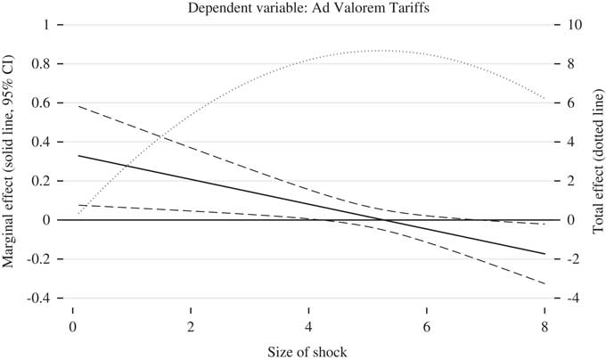
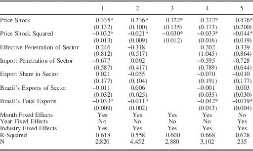
Since the model predicts an inverted-U shaped relationship between the intensity of a shock faced by an industry and the level of protection accorded to the industry, we test whether Price Shock > 0 and Price Shock Squared <0. Column 1 of Table 1 shows that the relationship between price shocks and tariffs accords well with our model’s predictions, as the coefficients are both statistically and substantively significant. At low levels of shocks, the more severe the shock to a particular industry, the more its tariffs increase. However, as shocks increase in size, tariffs peak and then fall back down. Figure 1 illustrates this relationship by using the specification provided in Column 1 to plot the marginal and total effects of price shocks on tariff policy outcomes. It shows that tariffs increase at a decreasing rate, and subsequently decrease at an increasing rate as shocks become more severe. The graph points to the statistical significance of our findings, yet the qualitative implications of these policy reformulations are also large. For example, a four-unit increase in the price shock raises tariffs by 8.2 percentage points overall. Given that the average tariff in our data is 25.6 per cent, an 8.2 percentage point increase represents a 32 per cent lift in the average tariff. As trade policy can have important consequences for growth, productivity, poverty and inequality, among a host of other measures,Footnote 105 the substantive ramifications of our results are potentially quite meaningful.
Marginal and total effect of industry shock as size of shock increases

Effect of Price Shock Intensity

Note: estimates from OLS regression. The dependent variable is the tariff rate for an industry. For Columns 1–4, the unit of observation is the industry-month, and for Column 5 the unit of observation is the industry-year. Robust standard errors, clustered by industry, appear in parentheses. Columns 1 and 3–5 use data covering 1986–95, while Column 2 uses data covering 1986–99. Column 3 excludes the control variables, and Column 4 lags the price shock by 2.5 years. Column 5 uses yearly price and tariff data. *p<0.05.
Table 1 also presents a variety of robustness checks that demonstrate that our results are not sensitive to particular model specifications. Column 2 uses extended data covering 1986–99.Footnote 106 Column 3 excludes control variables from the analysis, and Column 4 lags the price shock by two and a half years, rather than three years. Column 5 employs the specification from Table 1 but uses yearly price and tariff data.Footnote 107
We present additional robustness checks in the Appendix. First, we control for duration in our analysis. Brazil’s major banking and balance-of-payments crisis began in 1994, and was the largest and most relevant crisis during our period of analysis. We thus use an indicator of the number of years since the beginning of the crisis to measure crisis duration. We find that our results are strongly robust to this specification (see Table A4). Secondly, we use the Brazilian case to test our duration hypothesis by including both crisis duration and the square of this term. The results comport with our hypothesis and are statistically significant, although we urge caution in their interpretation because (as discussed earlier) Brazil experienced a variety of other crises through this period (Table A5). In each of these analyses, we find strong support for an inverted-U shaped relationship between the intensity of price shocks and subsequent tariff levels, as predicted by our theory. Although observational results such as those presented here should not be viewed as definitive, their robustness across specifications suggests real-world empirical patterns that accord with the core propositions of our theoretical model.
Tariffs and Shock Persistence
Our theory also predicts that following a shock, levels of protection exhibit an ‘up-down’ shape over time. We test this dynamic prediction using a cross-national sample, estimating the impact of crisis duration across 7,058 industries and sixteen countries from 1996 to 2010.
Model specification and results
As in our sub-national analysis, our dependent variable is an industry’s yearly ad valorem tariff rate within a country. These data were compiled from the World Trade Organization’s Tariff Download Facility and use the Harmonized System (HS) classification scheme.Footnote 108 In this analysis, to capture shocks to industries’ profitability, we specify our key independent variable as Crisis Duration. This variable indicates the number of years that have elapsed since the start of an economic crisis, as coded by Reinhart and Rogoff.Footnote 109 We code a crisis as occurring in a particular country-year if any of the crises identified by Reinhart and Rogoff are present in that country and year – including domestic defaults, external defaults, and banking, currency, stock market and inflation crises.Footnote 110 The duration of crises in our dataset persist for a minimum of one year and a maximum of thirteen years. Because we predict an inverted-U shaped relationship between tariff rates and the duration of the crisis, we also include Crisis Duration Squared. Additionally, we control for several time-varying factors that may influence trade policy response to crises including Log GDP, Log GDP Per Capita and Democracy,Footnote 111 along with country-industry and year fixed effects.Footnote 112 Summary statistics of the data can be found in the Appendix.
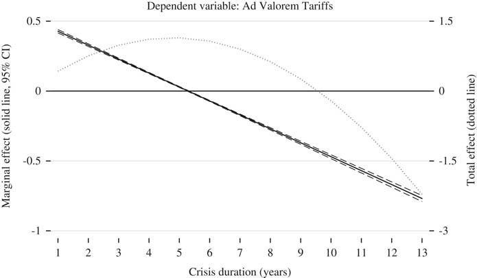
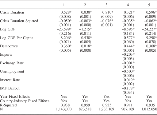
Column 1 of Table 2 demonstrates that, as predicted, the coefficient on Crisis Duration is positive and significant, while the coefficient on Crisis Duration Squared is negative and significant. Figure 2 plots the marginal effect of crisis duration on tariff policy outcomes using the specification provided in Table 2. Similar to Figure 1, it shows that tariffs increase at a decreasing rate, and subsequently decrease at an increasing rate as the durations of crises elongate. They peak five years after the onset of crises (increasing 1.14 percentage points), and then fall below initial levels as crises come to an end (decreasing 2.22 percentage points relative to the start). In other words, economic shocks of limited duration are associated with increased protection, whereas crises of greater duration lead to decreased protection and, eventually, liberalization. These findings are substantively important. The average tariff in our sample was 9 per cent; five years after the initiation of a crisis, the average tariff had increased by 12 per cent, while thirteen years after a crisis, the average tariff had decreased by 24 per cent. Qualitatively, these results accord with the narratives presented in the historical case studies discussed earlier.
Marginal and total effect of crisis duration as crisis duration increases

Temporal Effect of Price Shocks

Note: estimates from OLS regression. The unit of observation is the country-industry year, and the dependent variable is the tariff rate. In Column 2, the dependent variable is the logged tariff rate. The data cover 1996–2010. Robust standard errors, clustered by country-industry, appear in parentheses. All models include year and country-industry fixed effects, which are not shown. * p<0.05.
We conduct a variety of robustness checks to ensure that our results are not sensitive to a particular model specification. Column 2 shows that the results are robust to logging the dependent variable. Column 3 then removes all covariates, demonstrating that no particular control variable is driving our results.Footnote 113 Next, Column 4 includes a variety of variables that have been shown to impact trade liberalization. First, we control for the Exchange Rate, following a large literature arguing that movements in the exchange rate can influence trade protection.Footnote 114 Secondly, we include Imports, as import movements can alter demands for protection.Footnote 115 Thirdly, we control for the Unemployment Rate, as many scholars emphasize the potential impact of unemployment on trade protection.Footnote 116 Fourthly, we add a measure of the Interest Rate, which indicates the bank lending interest rate. Interest rates can impact tariff protection in a variety of ways; for example, when states have less leeway to manipulate interest rates, they may resort to raising tariffs as an alternative.Footnote 117 Lastly, IMF Bailout is an indicator of whether there was a positive International Monetary Fund (IMF) standby credit tranche balance, the main type of IMF assistance, in a given year. The IMF may condition its support on states’ trade liberalization,Footnote 118 so the presence of an IMF bailout is expected to decrease protection, which is indeed what we find.Footnote 119
Further, Column 5 removes the United States and the EU from the analysis, as they may focus on raising non-tariff barriers in response to requests for trade protection, even while most other nations rely primarily on tariff manipulation.Footnote 120 This may occur for two reasons. First, the implementation of non-tariff barriers requires a large bureaucratic capacity, while tariffs are straightforward to alter. Because the United States and the EU have such a capability, they may more heavily use these alternative routes of protection. Secondly, while most developing countries maintain tariff rates well below those bound by the WTO, the United States and the EU set tariff levels near these bounded levels.Footnote 121 Thus they may have less leeway to raise tariff barriers than other states. However, it is important to note that the United States and the EU still raise tariffs frequently in response to crises. The WTO provides a variety of exceptions that allow states to do so, particularly in times of economic hardship; countries often apply these safeguards well beyond the duration of a crisis.Footnote 122 In sum, while we retain the United States and the EU in our baseline analysis, we demonstrate the robustness of the results to their omission.Footnote 123
Heterogeneity and robustness
Our theoretical model predicts an inverted-U shaped relationship between crises and tariffs, yet it also provides additional testable hypotheses regarding industry-level characteristics. In particular, varying the intensity by which downstream producers’ profits are affected by changes in the domestic prices of input goods should have systematic implications for equilibrium tariffs. It is difficult to precisely measure this sensitivity parameter for each industry. One reasonable operationalization, however, involves comparing intermediate to final goods. For firms whose products are largely used as intermediate inputs in downstream production (compared to those that largely produce goods meant for final consumption), we expect the sensitivity of other firms to be higher. Given this interpretation of sensitivity, our model identifies two important characteristics of equilibrium tariffs. First, the inflection point in our inverted-U shaped relationship should occur earlier for intermediate goods than for final goods. Secondly, past this inflection point, equilibrium tariffs should fall more steeply for intermediate industries, because the greater sensitivity of downstream firms generates more costly counter-lobbying.
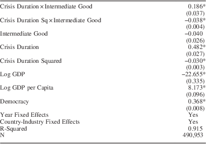
To test this subsidiary hypothesis, we collected data from the Global Trade, Assistance and Production database, which identifies, at the country-industry level, the total amount of production for that industry that was used as an intermediate product.Footnote 124 We then classify firms as above or below average in terms of their downstream usage, and created our measure of Intermediate Good that takes a value of 1 for industries above the mean, and 0 for those below. Given our theoretical expectation of different average effects of crises on trade protection for intermediate versus final goods, we add interaction terms between our crisis measure and our intermediate goods score to our primary specification.
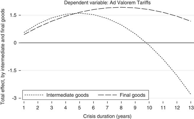
As can be seen in Table 3, we find strong support for our theoretical prediction on the heterogeneous effect of crises by degree of downstream usage for an industry. Recall that, as our formal model suggested that tariffs for intermediate industries should exhibit an earlier inflection point, and should decline faster past this point, this is mathematically equivalent to finding that the squared term on crisis duration should be more sharply negative than for final goods.Footnote 125 The interaction term between intermediate goods and the square of crisis duration is indeed statistically significant, and provides the predicted effect: for industries that produce intermediate goods, crises lead to declining tariffs at an earlier inflection point, and fall faster beyond this point. To see this more clearly, Figure 3 graphs the expected effect of crisis duration on tariffs for goods at low and high levels of downstream usage. Further, tariffs on industries characterized by more downstream usage peak sooner and fall faster than those on industries that primarily produce final products.
Total effect of crisis duration as crisis duration increases

Interaction with Intermediate Goods

Note: estimates from OLS regression. The unit of observation is the country-industry year and the dependent variable is the tariff rate. The data cover 1997–2010. Robust standard errors, clustered by country-industry, appear in parentheses. All models include year and country-industry fixed effects, which are not shown. *p<0.05.
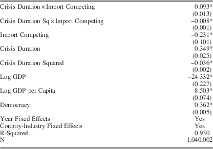
Given our empirical aim, in our theoretical model we restrict political competition in the face of a crisis to only occur around tariff rates. Yet in reality, some industries may pursue other policy options when faced with downturns in profitability. While an analysis of the full political portfolio of firms is beyond the scope of this article, this suggests an additional set of firm-level characteristics that should affect the heterogeneity of our results: the degree of import competition. For industries that do not face competing products from abroad, imposing a tariff on international goods should do little to shore up domestic profitability, implying that the relationship between economic crises and tariff rates should be much more pronounced for firms that face import competition. Following Kim’sFootnote 126 approach, we measured industry exposure to international competition using data on import elasticity from Broda and Weinstein.Footnote 127 We interact this measure with our linear and quadratic crisis duration terms to allow a differential effect for import-competing and non-import-competing industries. As can be seen in Table 4, we find strong support for this additional implication: while our inverted-U shape of tariffs remains for both sets of firms, equilibrium tariffs rise to much higher levels in response to a crisis among the subset of industries that faces international competition.Footnote 128
Import Competition

Note: estimates from OLS regression. The unit of observation is the country-industry year and the dependent variable is the tariff rate. The data cover 1997–2010. Robust standard errors, clustered by country-industry, appear in parentheses. All models include year and country-industry fixed effects, which are not shown. * p<0.05.
Further, anecdotal evidence appears to corroborate these systematic empirical patterns. Above, we presented qualitative evidence to show that when the US sugar industry lobbies for protection, the confectionary industry typically responds by counter-lobbying. Economic crises throw into sharp relief these lobbying and counter-lobbying dynamics. The sugar industry spent on average $3.8 million a year in lobbying expenses in the United States between 1998 and 2007.Footnote 129 The corresponding average for the confectionary industry was $2.2 million. After the onset of the 2007 financial crisis, however, sugar lobbying spiked to $7.5 million in 2008.Footnote 130 Importantly, there was no corresponding jump in lobbying by the confectionary industry immediately after the onset of the crisis: expenditures remained steady at $2.9 million in 2007, 2008 and 2009. Yet in line with our theory, spending in the confectionary industry subsequently jumped. In 2010, lobbying expenditures totaled $3.5 million (a 21 per cent increase); these sums remained high until the crisis abated.Footnote 131 While we only consider these descriptive empirical patterns to be suggestive, we note that they accord well with the lobbying and counter-lobbying dynamics that are central to our theoretical model.
Next, we investigate an additional implication of the model regarding lobbying behavior. The model predicts that at the start of a crisis, lobbying should increase by industries that produce intermediate goods, but as the crisis continues, industries that produce final goods should commence lobbying in response to the higher tariff rates placed on intermediate goods. Although data on lobbying patterns are difficult to obtain, we test this hypothesis using US lobbying data for the 2007–10 period, during which Reinhart and Rogoff code the United States as being in an economic crisis. As shown in Table A3, we find that, indeed, lobbying by industries that produced intermediate goods increased initially, followed by lobbying in other industries as the crisis wore on.
We perform a variety of additional robustness checks, the results of which are displayed in the Appendix due to space constraints. First, governments may be constrained in their ability to increase tariffs because of their WTO commitments, as they may only be able to raise tariffs up to their bound rates. As we explained above, however, this is unlikely due to the many escape clauses that allow members to violate these rules, particularly in times of economic duress. However, to ensure that these commitments are not driving our results, we (a) control for whether tariff rates were bound, (b) interact whether they were bound with our key independent variables and (c) conduct our analysis only on the subset of products that did have bound rates (Table A15). We find that our results are robust to each of these additional tests.
Additionally, we drop observations with residuals from our baseline specification greater than three or five times the standard deviation to ensure that the results are not driven by outliers (Table A8). We then condition on initial tariff levels, in case countries with higher initial tariff rates are less able to increase them in response to a crisis (Table A9). Next, we control for crisis intensity using a measure of the total number of crises that occurred in a given country in a given year, as coded by Reinhart and Rogoff (Table A10). We also employ an alternative measure of crisis duration, using within-country, industry-specific price shocks data from Datastream (Table A13). Further, given worries about the use of other forms of non-tariff barriers to trade, we demonstrate that our results hold when taking anti-dumping claims, and not tariff rates, as our dependent variable (Table A14). To summarize, we find strong and consistent support for our theoretically specified inverted-U shaped relationship between crises and trade protection across alternative modeling assumptions, different specifications of our outcome variable and empirical models that progressively add a host of important covariates – both within a given country across industries, and across industries and countries over time.
Conclusion
Existing research on the effects of crises on trade policy offers conflicting accounts, arguing at the same time that shocks make autarky more likely, that economic distress leads to less protectionism and that there is no systematic relationship linking crises to policy reform. Our novel theoretical account reconciles these diverging perspectives by distinguishing between the intensity and duration of economic shocks, and by explicating the differential effects of crises on industries’ lobbying resources and strategies. We demonstrate that as crises increase in severity, industries clamor for more protection, but when crises become dire, industries can no longer afford to secure protection because they must compete in the policy domain with other players seeking lower tariffs. Similarly, following the onset of a crisis, affected industries demand protection, but as the crisis persists over time, lobbying resources run dry and counter-lobbies mobilize to demand greater liberalization. We investigate our theory’s claims using formal modeling, illustrative examples, and both sub-national and cross-national empirical evidence, finding strong support for our argument.
Our results have several policy implications. For example, we find that when the cost of organizing a counter-lobby – a key parameter in our model – is lower, it is easier for firms to engage in counter-lobbying activities. These expenditures have a significant offsetting effect on the demand for trade protection, lowering tariff levels as shocks increase in size. To the extent that lower tariffs are desirable, then, reducing the organizational costs of counter-lobbying can result in more socially beneficial policy outcomes. More broadly, institutional designs that promote the broader representation of interest groups can achieve greater policy-making stability during crisis periods, as lobbying for policy adjustments can spark counter-lobbying that drives policy back toward the status quo. While our article does not speak directly to these implications, it raises a constructive set of research questions about the role of policy competition, institutional design and representation in shaping distributional politics.
Future work should examine how our theory pertains to other policy-making domains. While we focus on trade policy reactions to crises, our theory and research design could be used productively to investigate a variety of policy responses. For instance, previous work has explored the impact of lobbying expenditures on immigration, climate change, mortgage lending, tourism and university earmarks, to name just a few policy-making domains – yet these studies tend to focus only on lobbying activities that either promote or protect particular policies. Our study suggests, by contrast, that incorporating the role of offsetting special interests can result in very different theoretical predictions about how policies with distributional dimensions are contested in the political arena.
Furthermore, future research should also explore the heterogeneous treatment effects suggested by our theory. The strength of the U-shaped curve that we uncover may vary by institutional structures, for instance. Previous work has shown that countries with more veto points have a diminished ability to change pre-existing policies. Therefore, we might expect that these countries typically alter tariffs more slowly in response to crises. Conversely, countries with more access points might change policy more quickly, yet might also react more abruptly to countervailing pressures. By exploring these empirical implications systematically, scholars can shed new light on the dynamics of policy competition in diverse institutional domains.
We conclude by noting that our article suggests important extensions for the large body of work investigating crisis politics more generally. Understanding the conditions under which governments impose protection can shed light on the distributional consequences of a given crisis for different firms and industries in the economy, on shifts in public opinion over policy instruments and political representation, and on the strategies employed by industries in the midst of dynamic international and domestic economic changes. Our study implies that each of these processes is likely influenced by the duration and intensity of crises. By specifying the conditions under which crises spark lobbying and counter-lobbying, we offer a simple and parsimonious account that explains when and why industries lobby the government and attain their desired policy goals. In an era of repeated economic crises, our investigation of the political dynamics surrounding protection and reform is of particular importance, and is likely to remain of interest for the foreseeable future.
Appendix
Proof of Proposition 1
Our solution concept is sub-game perfect Nash equilibrium, and so we solve by backwards induction. A strategy for each industry
$i\in \left\{ {A,\,B} \right\}$
is to select a preferred tariff rate
 $\tau _{i} \in {\Bbb R}$
, as well as a lobbying schedule
 $l_{i} (\tau ):{\Bbb R}\to{\Bbb R}$
, that maps any value of
$$\tau $$
selected by the government onto the amount i will contribute. A strategy for government G is the choice of
 $\tau _{G} (l_{A} (\tau ),l_{B} (\tau )):{\Bbb R}^{2} \to{\Bbb R}$
, given the lobbying schedules of each industry, of a preferred tariff rate. An equilibrium of the game is composed of the optimal tariff rates and lobbying schedules for each industry (
 $\tau _{i}^{{\asterisk}} ,\,l_{i}^{{\asterisk}} (\tau _{i}^{{\asterisk}} )$
), as well as the government’s optimal tariff choice (
 $\tau _{G}^{{\asterisk}} $
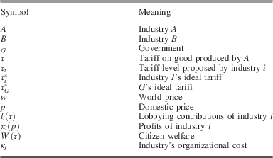
). A summary of our main variables is presented in Table A1.
Summary of Variables

We begin by investigating the government’s optimal decision. As a baseline, first consider G’s optimal response to A’s lobbying activity that does not induce B to counter-lobby; we precisely define the cut-point where this occurs below. In such an environment, G prefers to select some
 $$\tau \gt 0$$
whenever
 $l_{A} (\tau )\geq \hat l_{A}}(\tau )\,\equiv\,\left( {{\beta \over {1{\minus}\beta }}} \right)\gamma \tau .$
Rearranging, G selects
 $$\tau _{{\rm A}} $$
whenever
 $$l_{A} (\tau )\geq {\hat l}_{A} (\tau )\,\equiv\,\left( {{\beta \over {1{\minus}\beta }}} \right)\gamma \tau .$$
Knowing that it can secure G’s support for a given
$$\tau $$
by contributing at least
 $\hat l_{A} (\tau )$
, A never offers more than this amount in equilibrium. Thus, A faces a trade-off whereby its profits are increasing in
$$\tau $$
(
 $$\partial \pi _{A} {\rm /}\partial \tau \gt 0$$
), but the costs associated with compensating G for this protection are also increasing in
 $\tau \left( {\partial \hat l_{A} /\partial \tau \gt 0} \right)$
. As is standard, A’s best response is to select the
$$\tau _{{\rm A}} $$
that exactly equates the marginal increase in
$\pi _{A} (p)$
from increased p with the marginal increase in
 $l_{A} (\tau )$
; call the p where this occurs
$\hat{p}$
Put differently,
$\hat{p}$
gives the p at which the weighted-welfare cost curve is precisely tangent to A’s profit function. Given our assumption of linearity for the losses in W (
$$\tau $$
) associated with
$$\tau $$
, we may define this formally as:
 $${{\partial \pi _{A} } \over {\partial p}}{\Big |} {_{{\hat{p}}} } =\left( {{\beta \over {1{\minus}\beta }}} \right)\gamma .$$
Note that when
 $w\gt \hat{p}$
, A provides no
 $l_{A} (\tau )$
, as the marginal loss of W (
$$\tau $$
) arising from increased
$$\tau $$
outstrips any marginal
$\pi _{A} (p)$
gained from increasing p. Thus when the intensity of a shock is ‘small’, in equilibrium, no
 $l_{i} (\tau )$
is offered and G maintains
 $$\tau =0$$
. Formally:
Equilibrium 1: When
 $w\gt \hat{p}$
:
 $$\tau _{A}^{{\asterisk}} =\tau _{B}^{{\asterisk}} =\tau _{G}^{{\asterisk}} =l_{A}^{{\asterisk}} (\tau )=l_{B}^{{\asterisk}} (\tau )=0.$$
However, when w falls below
$\hat{p}$
, it becomes profitable for A to seek the
$$\tau $$
that raises p precisely to
$\hat{p}$
That is, A’s profit-maximizing
$$\tau $$
is
 $\tau _{A}^{{\asterisk}} =\hat{p}{\minus}w$
; to repeat, this is the
$$\tau $$
at which the marginal costs associated with a higher
$$\tau $$
exactly equals the marginal
$\pi _{A} (p)$
associated with increased p. Having selected this ideal rate, A then offers l
A
(
$$\tau $$
*) to G to compensate it for the loss of W (
$$\tau $$
) associated with
$\tau _{A}^{{\asterisk}} $
.
Before stating the equilibrium results of this case, we must identify the threshold level of
$$\tau $$
at which B counter-lobbies. Note that when both A and B provide (positive) l
i
(
$$\tau $$
) to G, G selects
 $\tau _{B} \lt \tau _{A} $
whenever
 $\beta W(\tau _{B} ){\plus}(1{\minus}\beta )l_{B} (\tau _{B} )\geq \beta W(\tau _{A} ){\plus}(1{\minus}\beta )l_{A} (\tau _{A} )$
.Footnote
132
Rearranging terms, G selects
 $$\tau _{{\rm B}} $$
whenever
 $$l_{B} (\tau _{B} )\geq \hat l_{B} (\tau _{B} )\,\equiv\,l_{A} (\tau _{A} ){\minus}\left( {{\beta \over {1{\minus}\beta }}} \right)[\gamma \tau _{B} {\plus}\gamma \tau _{A} ].$$
Note that B’s optimal tariff rate is always zero: π
B
(p) is a declining function of
$$\tau _{{\rm B}} $$
, as are the l
B
(
$$\tau $$
) required to convince G to support
$$\tau _{{\rm B}} $$
, and so selecting
 $\tau _{B}^{{\asterisk}} =0$
is its unique best response. Thus in what follows, we replace
$$\tau _{{\rm B}} $$
with zero. Making this substitution into Equation 10, and recalling the definition of
 $$\hat l_{A} (\tau _{A} )$$
from Equation 8, the cost associated with securing G’s support for B is
 $$l_{B} (0)\geq \hat l_{B} (0)\,\equiv\,l_{A} (\tau _{A} ){\minus} \hat l_{A} (\tau _{A} ).$$
Similar to the discussion of A’s lobbying decision above, if B knows it can secure G’s support by contributing at least
 $\hat l_{B} (0)$
, it never offers more in equilibrium, so whenever B secures G’s support, it contributes exactly
$\hat l_{B} (0)$
.
We can now precisely describe the cut-off point at which increasing
$$\tau $$
induces counter-lobbying. Recall that when B does not enter the counter-lobby market (assuming that
 $w\lt \hat{p}$
), A contributes exactly
 $\hat l_{A} \left( {\tau _{A}^{{\asterisk}} =\hat{p}{\minus}w} \right)$
. As B must pay κ
B
to organize in order to counter-lobby, there always exists a segment of the parameter space where the gains B would receive from entering the counter-lobbying market would not offset κ
B
. However, we may define
$\hat{w}$
as the value of w at which, should A maintain its strategy of lobbying for
 $\tau _{A}^{{\asterisk}} =\hat{p}{\minus}w$
by contributing
 $\hat l_{A} \left( {\tau _{A}^{{\asterisk}} } \right)$
, B is perfectly indifferent between remaining out of the lobbying market, or entering.Footnote
133
Formally, we define
$\hat{w}$
as the value of w at which
 $$\sigma \pi _{B} (\hat{w}){\minus}\kappa _{B} =\sigma \pi _{B} (\hat{p}).$$
To be clear: when
$w\geq \hat{w}$
, the benefits B derives from counter-lobbying are always outweighed by the costs of doing so, and so in this range, A can always obtain
$\tau _{A}^{{\asterisk}} $
without facing counter-lobby pressure. Thus when the intensity of a shock is ‘moderate’, A is able to secure
$\tau _{A}^{{\asterisk}} $
by compensating G for the associated distortions to W (
$$\tau $$
), and B does not find it profitable to enter the counter-lobby market in equilibrium. Formally:
Equilibrium 2: Whenever
 $\hat{w}\leq w\leq \hat{p}$
:
 $$\tau _{A}^{{\asterisk}} =\hat{p}{\minus}w,\,l_{A}^{{\asterisk}} \left( {\tau _{A}^{{\asterisk}} } \right)=\hat l_{A} \left( {\tau _{A}^{{\asterisk}} } \right),\,\tau _{B}^{{\asterisk}} =l_{B}^{{\asterisk}} (\tau _{B}^{{\asterisk}} )=0,\,and\,\tau _{G}^{{\asterisk}} =\tau _{A}^{{\asterisk}} .$$
In this equilibrium space, for shocks of greater intensity (that is, for lower values of w), the equilibrium level of
$$\tau $$
increases.
Yet when
$w\lt \hat{w}$
, B may find it profitable to enter the counter-lobbying market. Having determined the l
B
(
$$\tau $$
) it must offer to win G’s support, B prefers to do nothing rather than to engage in counter-lobbying whenever
 $\pi _{B} (w){\minus}\kappa _{B} {\minus} \hat l_{B} (0)\leq \pi _{B} (w{\plus}\tau _{A} )$
. Rearranging, and substituting for
$\hat l_{B} (0)$
, A successfully deters B from counter-lobbying by setting
 $$l_{A} (\tau _{A} )\geq \hat l_{A} ^{\prime} (\tau _{A} )\,\equiv\,\sigma (\pi _{B} (w){\minus}\pi _{B} (w{\plus}\tau _{A} )){\minus}\kappa _{B} {\plus} \hat l_{A} (\tau _{A} ).$$
As above, in any equilibrium in which A successfully out-lobbies B, it contributes exactly this amount, as any additional contributions make A strictly worse off without further changing the equilibrium
$$\tau $$
. However, facing a potential counter-lobbying threat from B, A also possesses an alternative strategy: rather than selecting a higher
$$\tau $$
and outbidding B in order to win G’s support, it may instead select a lower ‘compromise’ level of
$$\tau $$
that does not trigger B’s counter-lobbying, thereby reducing the l
A
(
$$\tau $$
) associated with winning G’s support. For any w, there always exists some
$\tilde{\tau }$
, such that if A contributes its ‘non-competition’ offer of
 $\hat l_{A} (\tilde{\tau })$
, B is indifferent between entering the counter-lobbying market and staying out. Formally, we define
$\tilde{\tau }$
such that
 $$\sigma \pi _{B} (w){\minus}\kappa _{B} =\sigma \pi _{B} (w{\plus}\tilde{\tau }).$$
In this final case, A’s optimal strategy depends on a comparison of the pay-off it would receive by setting
 $\tau _{A} \gt \tilde{\tau }$
, thereby necessitating additional l
A
(
$$\tau $$
) to successfully outbid B, or instead accepting a lower
$\tilde{\tau }$
that would not provoke counter-lobbying pressure from B. A prefers to accept
$\tilde{\tau }$
whenever
 $\pi _{A} (w{\plus}\tau _{A} ){\minus}\hat l_{A} ^{\prime} (\tau _{A} )\leq \pi _{A} (w{\plus}\tilde{\tau }){\minus}\hat l_{A} (\tilde{\tau })$
which, following substitution and rearrangement, gives
 $$\pi _{A} (w{\plus}\tau _{A} ){\minus}\pi _{A} (w{\plus}\tilde{\tau })\leq \left( {{\beta \over {1{\minus}\beta }}} \right)\gamma \left[ {\tau _{A} {\minus}\tilde{\tau }} \right]{\plus}\sigma (\pi _{B} (w){\minus}\pi _{B} (w{\plus}\tau _{A} )){\minus}\kappa .$$
Thus whenever Equation 15 holds, A selects
$\tilde{\tau }$
and avoids counter-lobbying pressure from B; when Equation 15 does not hold, A instead selects a higher ideal
$$\tau $$
A
that maximizes its profits conditional on allowing it to outbid B (denoted
 $\hat{\tau }$
), and provides additional l
A
(
$$\tau $$
) to secure G’s support. In other words, when the intensity of the shocks is ‘severe’, A may prefer to either select
$\tilde{\tau }$
to avoid counter-lobbying pressure, or it may instead select
$\hat{\tau }$
, which requires it to contribute additional l
A
(
$$\tau $$
) to successfully outbid B. Formally:
Equilibrium 3: Whenever
$w\lt \hat{w}$
and Equation 15 holds:
 $\tau _{A}^{{\asterisk}} =\tilde{\tau }$
,
 $l_{A}^{{\asterisk}} \left( {\tau _{A}^{{\asterisk}} } \right)=\hat l_{A} \left( {\tau _{A}^{{\asterisk}} } \right)$
,
 $\tau _{B}^{{\asterisk}} =0$
,
 $l_{B}^{{\asterisk}} (0)=\hat l_{B} (0)$
, and
 $\tau _{G}^{{\asterisk}} =\tau _{A}^{{\asterisk}} $
. Whenever
$w\lt \hat{w}$
and Equation 15 does not hold:
 $\tau _{A}^{{\asterisk}} =\hat{\tau }$
,
 $l_{A}^{{\asterisk}} \left( {\tau _{A}^{{\asterisk}} } \right)=\hat l_{A} ^{\prime} \left( {\tau _{A}^{{\asterisk}} } \right)$
,
$\tau _{B}^{{\asterisk}} =0$
,
$l_{B}^{{\asterisk}} (0)=\hat l_{B} (0)$
, and
$\tau _{G}^{{\asterisk}} =\tau _{A}^{{\asterisk}} $
.
The discussion of how
$$\tau $$
responds to more severe shocks in equilibrium requires one final clarification: several of the terms within Equation 15 are themselves functions of w, and so the likelihood that this condition holds may vary with w. Note that if Equation 15 holds, as soon as
$w\lt \hat{w}$
,
$\tilde{\tau }$
is selected in equilibrium.
$\tilde{\tau }$
declines as w continues to fall,Footnote
134
so when A immediately chooses
$\tilde{\tau }$
, in equilibrium
$$\tau $$
declines for a shock of greater intensity. If characterized by these conditions, this completes the proof for
$$\tau $$
that rises for shocks of moderate intensity, but declines for shocks of severe intensity.
However, if Equation 15 does not initially hold, in equilibrium,
$$\tau $$
continues to increase in shock intensity until the condition finally binds. To see this, note that A’s pay-off from setting a higher tariff
$\tau _{A} \gt \tilde{\tau }$
and then outbidding B is
 $\pi _{A} (w{\plus}\tau _{A} ){\minus}\hat l_{A} ^{\prime} \left( {\tau _{A} } \right)$
which, substituting, is
 $$u_{A} (\tau _{A} )=\pi _{A} (w{\plus}\tau _{A} ){\minus}\sigma (\pi _{B} (w){\minus}\pi _{B} (w{\plus}\tau _{A} )){\plus}\kappa _{B} {\minus}\left( {{\beta \over {1{\minus}\beta }}} \right)\gamma \tau _{A} .$$
Under the assumption that
 $\partial u_{A} /\partial \tau _{A} \gt 0$
,Footnote
135
as u
A
(
$$\tau _{{\rm A}} $$
) is composed of both concave and convex functions of
$$\tau _{{\rm A}} $$
,
 $\hat{\tau }_{{\rm A}} $
depends on which of these two effects dominates. That is, if u
A
(·) is concave in
$$\tau _{{\rm A}} $$
,
$\hat{\tau }$
is that which satisfies the standard first order condition such that
 $\partial u_{A} /\partial \hat{\tau }=0$
, which occurs when
 $${{\partial \pi _{A} } \over {\partial p}}{\plus}{{\partial \pi _{B} } \over {\partial p}}{\minus}\left( {{\beta \over {1{\minus}\beta }}} \right)\gamma =0.$$
As Equation 17 only declines in w so long as u
A
(·) is concave,Footnote
136
$\hat{\tau }$
increases in magnitude as w falls.
Yet if u
A
(·) is convex in
$$\tau _{{\rm A}} $$
,
$\tau _{A}^{{\asterisk}} $
lies on either of the boundary conditions. If this exists at the lower bound of zero, then clearly A would instead be better off by selecting
$\tilde{\tau }$
. However, the upper bound of
$\tau _{A}^{{\asterisk}} $
is the same as that which maximizes
$\pi _{A} (p)$
when not facing counter-lobby pressure, which is the
$$\tau $$
that exactly equates p with
$\hat{p}$
.
In either case, then, as long as A prefers to set
 $\tau \,\ne\,\tilde{\tau }$
and outbid B, in equilibrium,
$$\tau $$
continues to increase in shock intensity. However, as long as the right-hand-side components of Equation 15 increase at a faster rate than the left-hand-side components, shocks of increased intensity eventually lead Equation 15 to bind, leading
$\tilde{\tau }$
to be chosen in equilibrium rather than
$$\tau $$
, which subsequently declines in shock intensity.
Thus it is only in the case where π
A (p)’s elasticity (the left-hand component of Eq. 15) is so extreme that it outpaces the costs of offsetting not only the additional losses of W (
$$\tau $$
) arising from higher
$$\tau $$
, but also the additional π
B (p) lost to B (the right-hand components of Eq. 15) that a switch to
$\tilde{\tau }$
does not occur. While we identify this equilibrium outcome for the sake of theoretical completeness, A and B are not likely to always maintain profitability in the market when faced with catastrophic shocks; the addition of a budget constraint in the subsequent version of the game helps address this somewhat strange segment of the parameter space.
Proof of Proposition 2
Our solution concept is Markov Perfect Equilibrium, taking ρ
t
as the state variable.Footnote
137
A strategy for each industry
$i\in \left\{ {A,\,B} \right\}$
is to select, in each period t, a tariff rate
 $\tau _{{it}} \in {\Bbb R}$
, as well as a lobbying schedule
 $l_{{it}} (\tau ):{\Bbb R}\to{\Bbb R}$
, that maps the contribution it makes to G should a particular value of
$$\tau $$
be selected. A strategy for G is the choice in each period of
 $\tau _{{Gt}} :{\Bbb R}^{2} \to{\Bbb R}$
, given
 $l_{{it}} (\tau _{t} )$
. An equilibrium of the game is composed of the optimal tariff rates and lobbying schedules for each industry (
 $\tau _{{it}}^{{\asterisk}} ,\,l_{{it}}^{{\asterisk}} (\tau _{{it}}^{{\asterisk}} )$
), as well as G’s optimal tariff choice (
 $\tau _{{Gt}}^{{\asterisk}} $
).
In the first period of the game, we assume that A has accrued some additional outside resources of amount ρ 1, which are given exogenously. In each subsequent period, these available outside resources are defined simply as any residual profits from play in the previous round; formally,
 $$\rho _{{t{\plus}1}} =\pi _{A} (\tau _{t} ){\plus}\rho _{t} {\minus}l_{{At}} (\tau _{t} ).$$
Observe that ρ t+1 is equivalent to A’s period pay-off in t; as a consequence, A does not face an inter-temporal trade-off. That is, while it might be possible that A would want to save additional resources for expected future payments, as future outside resources are maximized by maximizing current pay-offs, A’s long-run best response is equivalent to repeatedly solving its single-period maximization problem. As such, the within-period equilibria of our repeated game are largely identical to those described in the Proof of Proposition 1, save one major alteration. Rather than repeat the explanation of each equilibrium here, we instead note the changes that arise in each equilibrium.
Changes to Equilibrium 1 (
 $\hat{p}\lt w$
)
In Equilibrium 1, the imposition of a budget constraint does not affect the outcome, as there is no lobbying activity.
Changes to Equilibrium 2 (
$\hat{w}\leq w\leq \hat{p}$
)
In Equilibrium 2, the imposition of a budget constraint requires that A must be able to afford
 $\tau _{{At}}^{{\asterisk}} $
. Recall that, in Equilibrium 2, A does not face counter-lobbying pressure from B, and so its lobbying costs are only those that arise from compensating G for losses associated with W (
$$\tau $$
) that arise from trade protection. Given A’s ideal tariff
 $\tau _{{At}}^{{\asterisk}} =\hat{p}{\minus}w$
, and recalling the definition of the lobbying amount required to win G’s approval
 ${\hat l}_{{At}} (\tau )$
from Equation 8, if
 $\pi _{A} (\tau _{{At}}^{{\asterisk}} )\geq \left( {{\beta \over {1{\minus}\beta }}} \right)\gamma \tau _{{At}}^{{\asterisk}} $
, then A can afford to lobby G for
$\tau _{{At}}^{{\asterisk}} $
simply through same-period profits, and there is no change in the within-period equilibrium result. In addition, since A’s profitability is completely sufficient to cover any lobbying costs, there are no temporal dynamics as the stage game is repeated: if A could afford
$\tau _{{At}}^{{\asterisk}} $
without needing ρ
t
, it can clearly still secure
$\tau _{{At}}^{{\asterisk}} $
in subsequent rounds.
Yet if
 $\pi _{A} (\tau _{{At}}^{{\asterisk}} )\lt \left( {{\beta \over {1{\minus}\beta }}} \right)\gamma \tau _{{At}}^{{\asterisk}} $
, then same-period profits are not sufficient to cover the l
At
(
$$\tau $$
) that arise from securing
$\tau _{{At}}^{{\asterisk}} $
. In this case, if
 $\rho _{t} \lt \left( {{\beta \over {1{\minus}\beta }}} \right)\gamma \tau _{{At}}^{{\asterisk}} {\minus}\pi _{A} (\tau _{A}^{{\asterisk}} )$
, then A cannot afford
$\tau _{{At}}^{{\asterisk}} $
even by dipping into its ‘war chest’. In this case, A’s best response is to choose to exit the market, earning an outside pay-off of zero forever.Footnote
138
In such a case, absent lobbying pressure for trade protection from A, G selects
 $$\tau _{t} =0$$
, thereby maximizing W (
 $$\tau _{t} $$
).
If, instead,
 $\rho _{t} \geq \left( {{\beta \over {1{\minus}\beta }}} \right)\gamma \tau _{{At}}^{{\asterisk}} {\minus}\pi _{A} (\tau _{A}^{{\asterisk}} )$
, then A can still afford
$\tau _{{At}}^{{\asterisk}} $
by making use of ρ
t
. In this case, the within-period equilibrium remains unchanged. However, this raises the possibility of an over-time dynamic regarding crises of extended duration. In particular, given the definition of future outside resources as simply the remainder of previous period profits, and noting that, in the space under consideration,
 $\pi _{A} (\tau _{{At}}^{{\asterisk}} ){\minus}\left( {{\beta \over {1{\minus}\beta }}} \right)\gamma \tau _{{At}}^{{\asterisk}} \lt 0$
, it must be that ρ
t+1<ρ
t
.
Consideration of A’s optimal strategy in time t + 1 depends critically on how severely ρ
t+1 has been depleted by first-period lobbying. If, in time t + 1, it is still the case that
 $\rho _{{t{\plus}1}} \geq \left( {{\beta \over {1{\minus}\beta }}} \right)\gamma \tau _{{At{\plus}1}}^{{\asterisk}} {\minus}\pi _{A} (\tau _{{At{\plus}1}}^{{\asterisk}} )$
, then equilibrium tariffs remain unchanged. If, instead,
 $\rho _{{t{\plus}1}} \lt \left( {{\beta \over {1{\minus}\beta }}} \right)\gamma \tau _{{At{\plus}1}}^{{\asterisk}} {\minus}\pi _{A} (\tau _{{At{\plus}1}}^{{\asterisk}} )$
, then A will not be able to secure
 $\tau _{{At{\plus}1}}^{{\asterisk}} $
, and so will choose to exit the market, leading to a reduction in tariffs.
While so far we have considered how equilibrium tariffs might change in a two-period setting, it is easy to generalize our predictions to additional periods. More generally, we may define the per-period loss in outside resources as
 $\Delta \rho _{t} =\left( {{\beta \over {1{\minus}\beta }}} \right)\gamma \tau _{{At}}^{{\asterisk}} {\minus}\pi _{A} \left( {\tau _{{At}}^{{\asterisk}} } \right)$
. For any fixed amount of resources available to A at the start of the game (ρ
1), the resources available to it in the nth round will simply be
 $\rho _{1} {\minus}\left( {n{\minus}1} \right)\Delta \rho _{t} $
. As this decreases continually over time, extending the crisis to additional periods increases the likelihood that A can no longer afford
$\tau _{{At}}^{{\asterisk}} $
, thereby pushing it out of the market and returning
$$\tau $$
to its pre-crisis level. Thus while
$$\tau $$
is likely to increase at the outset of a crisis, as a crisis extends in duration, the likelihood that industries may be able to maintain this
$$\tau $$
diminishes, suggesting that in equilibrium,
$$\tau $$
should subsequently fall as the duration of a crisis is extended.
Changes to Equilibrium 3 (
$w\lt \hat{w}$
)
In Equilibrium 3, the imposition of a budget constraint introduces the same potential over-time dynamic as in Equilibrium 2. Specifically, if Equation 15 holds, then we must determine whether A can afford the ‘compromise’ tariff identified in Equation 14, either with or without recourse to ρ
t
. If Equation 15 does not hold, we instead must determine whether A can afford its ‘out-bidding’ tariff
$\hat{\tau }$
, either with or without the use of ρ
t
. In either case, if A can secure
$\tau _{{At}}^{{\asterisk}} $
without needing to make use of ρ
t
, then there is no change in the equilibrium outcome, so long as
 $\pi _{A} \left( {\tau _{A}^{{\asterisk}} } \right){\minus}\left( {{\beta \over {1{\minus}\beta }}} \right)\gamma \tau _{{At}}^{{\asterisk}} \geq 0$
.
Yet if A cannot afford
$\tau _{{At}}^{{\asterisk}} $
simply from within-period profits, then depletion of ρ
t
over time, as given by Δρ
t
, may mean that in future periods, A will no longer be able to afford the lobbying costs associated with trade protection, and will exit the market, leading G to reimpose
 $$\tau {\rm =0}$$
. As a crisis extends in duration to additional periods, for a fixed ρ
1
, the likelihood that
 $\pi _{A} \left( {\tau _{{At}} } \right){\plus}\rho _{t} \lt \left( {{\beta \over {1{\minus}\beta }}} \right)\gamma \tau _{{At}} $
increases. Thus again, we expect that while
$$\tau $$
increases at the outset of a crisis, as the crisis extends in duration, industries lose their ability to maintain trade protection, suggesting that the equilibrium
$$\tau $$
subsequently falls as the duration of a crisis is extended.
Proof of sectoral sensitivity comparative statics
We discuss immediately below the effect of changes in the sensitivity of profits in industry B (σ) to increases in the price of good A within each equilibrium, as detailed above.
Changes to Equilibrium 1 (
$\hat{p}\lt w$
)
For ‘very small’ shocks, it is not in A’s best interest to lobby at all; this equilibrium is not affected by changes in σ.
Changes to Equilibrium 2 (
$\hat{w}\leq w\leq \hat{p}$
)
Once the world price falls enough to induce lobbying activity by A, the sensitivity of downstream producers becomes an important component of equilibrium play. Recall from above that, so long as
 $\hat{w}\leq w$
, A can set its ideal tariff rate without triggering counter-lobbying activity by B. Given the utility function for B, we define
$\hat{w}$
such that
 $\sigma \pi _{B} (\hat{w}){\minus}\sigma \pi _{B} (\hat{p})=\kappa _{B} $
, which is equivalent to
 $$\pi _{B} (\hat{w}){\minus}\pi _{B} (\hat{p})={{\kappa _{B} } \over \sigma }.$$
Given fixed
$\hat{p}$
and κ
B
, an increase in σ will result in a greater value for
$\hat{w}$
; that is,
 $\partial \hat{w}/\partial \sigma \gt 0$
. Intuitively, when downstream firms are affected more severely by a change in the price of upstream goods (higher σ), there will be a smaller range wherein A can successfully lobby for increasing tariffs without facing counter-lobbying. However, when the sensitivity of other firms to the price of A is low (smaller σ), there will be a wider range of shocks where A can lobby for its ideal (higher) tariff rate without facing counter-lobbying pressure. In essence, the sensitivity of B to prices in A affects the range of shock sizes where Equilibrium 2 holds: as σ increases, this equilibrium becomes less likely, whereas when σ declines, this equilibrium holds for a wider segment of the parameter space.
Changes to Equilibrium 3 (
$w\lt \hat{w}$
)
Finally, beyond making Equilibrium 3 (when counter-lobby pressure becomes a binding factor on A) more likely to hold generally, the sensitivity of downstream firms also affects A’s optimal strategy once it faces counter-lobbying. Recall that, once counter-lobbying by B becomes credible (when
$w\lt \hat{w}$
), A now chooses between setting a ‘compromise’ tariff that leaves B indifferent between counter-lobbying or not, or instead chooses an ‘out-bidding’ tariff that induces B to make a counter-lobby offer, but which is large enough to still secure government support (despite the possibility of an offer from B). In the first case, the compromise tariff
$\tilde{\tau }$
is defined such that
 $\sigma \pi _{B} (w){\minus}\kappa _{B} =\sigma \pi _{B} (w{\plus}\tilde{\tau })$
, which can be rearranged as:
 $$\pi _{B} (w){\minus}\pi _{B} (w{\plus}\tilde{\tau })={{\kappa _{B} } \over \sigma }.$$
For fixed w and κ
B
, any increase in σ must result in a decrease in
$\tilde{\tau }$
; that is, when downstream firms are more sensitive to price changes in A, the ‘compromise’ tariff they will accept is lower than those that would appease firms that are only weakly affected by prices in A (or,
 $\partial \tilde{\tau }/\partial \sigma \lt 0$
). This suggests that, not only does greater sensitivity decrease the range over which A can secure rising tariffs, it also accentuates the rate of decline in compromise tariffs in Equilibrium 3.
Alternately, A may choose to instead outbid B and secure a higher tariff
$\tau _{A} \gt \tilde{\tau }$
; A’s pay-off for doing so is:
 $$u_{A} (\tau _{A} )=\pi _{A} (w{\plus}\tau _{A} ){\minus}\sigma (\pi _{A} (w)){\minus}\pi _{B} (w{\plus}\tau _{A} ){\plus}\kappa _{B} {\minus}\left( {{\beta \over {1{\minus}\beta }}} \right)\gamma \tau _{A}. $$
Observe that, as B becomes more sensitive to changes in the price of A, the additional lobbying amount that A must provide is increased; that is, as A must sacrifice additional resources to compensate the government for giving up larger counter-lobby offers from a more sensitive B, A’s own pay-off declines monotonically in σ. This suggests, again, that even when A chooses to outbid B, its pay-off from doing so will fall when B is more sensitive to prices in A.
Overall effect of sensitivity
Combining the points made above, we now characterize the general effects of changes in the sensitivity of B to price changes in A. For more sensitive firms (higher σ), we expect the inflection point at which equilibrium tariffs move from rising to falling in shock intensity to occur earlier – this arises by compressing the parameter space over which Equilibrium 2 (in which greater shocks correspond to rising equilibrium tariffs) holds. Additionally, we expect that, once equilibrium tariffs have begun to fall, the rate of decline of these tariffs past the inflection point will be sharper. This arises because greater sensitivity by B drives down both the outbid and the compromise tariffs selected by A in Equilibrium 3.
More generally, if we take firms producing intermediate goods as those most likely to face downstream industries with greater sensitivity, this suggests that our inverted-U prediction regarding equilibrium tariff rates should be more pronounced for intermediate industries. Yet for industries that primarily produced final goods, the overall sensitivity of other producers to prices in the markets of final goods should be weaker, suggesting that the inflection point for counter-lobbying should be much lower, and experience a much more gradual decline in equilibrium tariffs after the inflection.