1 Introduction
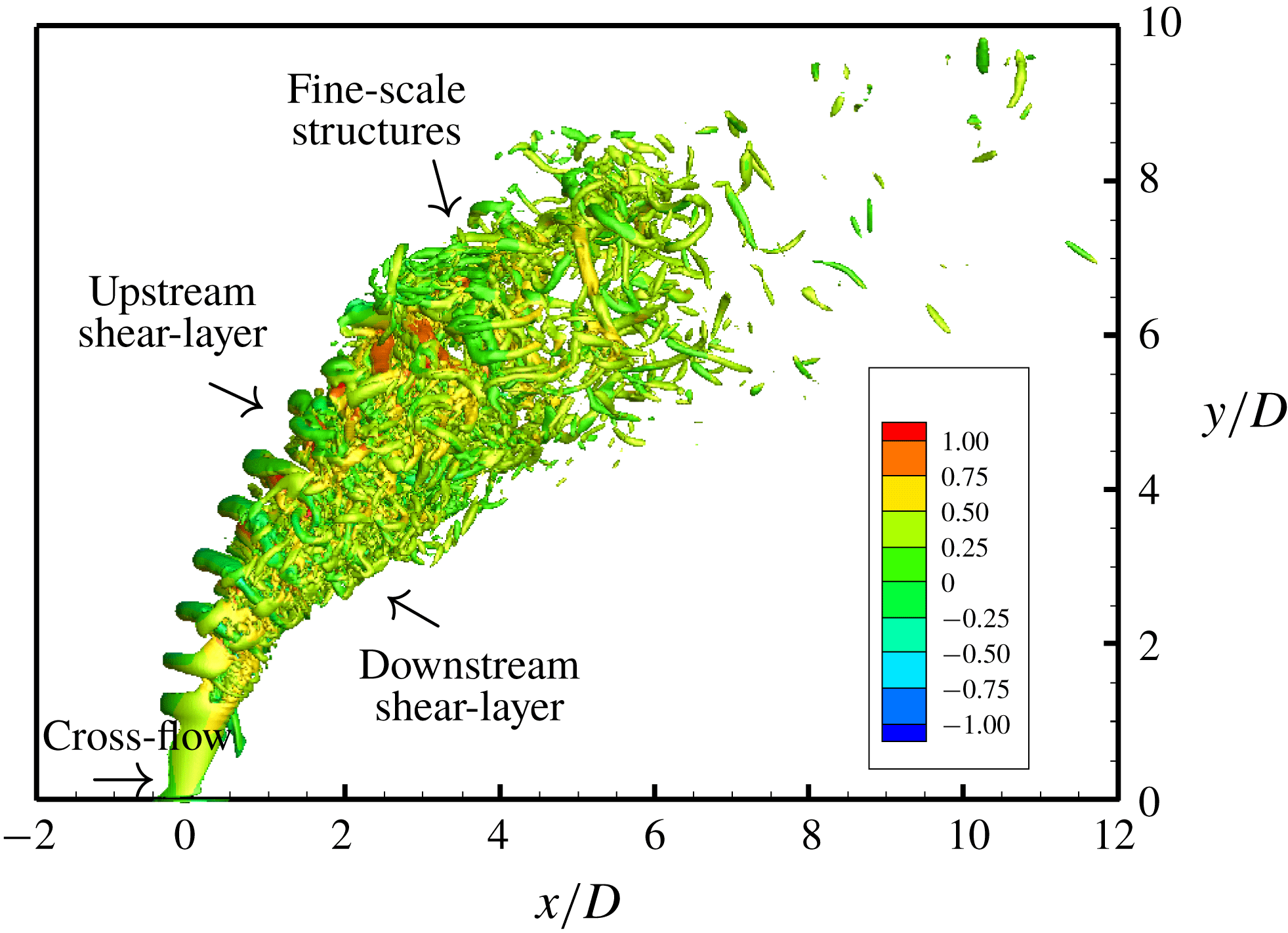
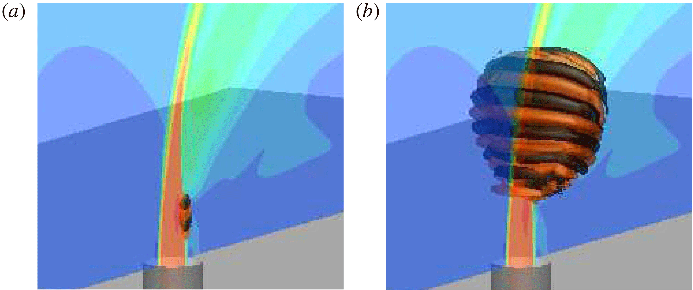
Jet in cross-flow (JICF) or transverse jet is a common flow problem characterized by a jet of fluid injected normal to a cross-flow. Often the cross-flow consists of a planar boundary layer which interacts with the jet of fluid creating complex vortical structures. Figure 1 shows an instantaneous flow field of a typical JICF visualized using isocontour of
 $Q$
-criterion (Hunt, Wray & Moin Reference Hunt, Wray and Moin1988) coloured with streamwise velocity. The upstream and downstream shear layers are marked for clarity. The shear-layer vortices and Kelvin–Helmholtz instability can be observed along the upstream side of the jet path. Kamotani & Greber (Reference Kamotani and Greber1972) and Smith & Mungal (Reference Smith and Mungal1998) observed the counter-rotating vortex pair (CVP) dominating the jet cross-section and travelling far downstream. Horseshoe vortices (Krothapalli, Lourenco & Buchlin Reference Krothapalli, Lourenco and Buchlin1990; Kelso & Smits Reference Kelso and Smits1995) form near the wall around the upstream side of the jet nozzle exit. They travel downstream and begin to tilt upward during ‘separation events’ (Fric & Roshko Reference Fric and Roshko1994) due to the adverse pressure gradient caused by jet entrainment. These wall-normal vortical structures that extend through the jet wake are described as wake vortices (McMahon, Hester & Palfery Reference McMahon, Hester and Palfery1971; Moussa, Trischka & Eskinazi Reference Moussa, Trischka and Eskinazi1977; Fric & Roshko Reference Fric and Roshko1994; Eiff, Kawall & Keffer Reference Eiff, Kawall and Keffer1995; Kelso, Lim & Perry Reference Kelso, Lim and Perry1996).
Instantaneous flow field for a JICF visualized using isocontours of
 $Q$
-criterion coloured by streamwise velocity showing the upstream and downstream shear layers.

Transverse jets are found in many engineering applications, e.g. dilution jets in gas turbine combustors, film cooling of turbine blades and the thrust vectoring mechanism of vertical and/or short take-off and landing aircraft. Readers are referred to Margason (Reference Margason1993), Karagozian (Reference Karagozian2010) and Mahesh (Reference Mahesh2013) for comprehensive reviews of JICF research, both experimental and computational, over the last seven decades.
An incompressible JICF can be characterized by the jet Reynolds number (
 $Re$
), the cross-flow Reynolds number (
 $Re_{\infty }$
) and the JICF velocity ratio (
 $R$
) defined as
 $$\begin{eqnarray}\displaystyle & \displaystyle Re=\overline{v}_{jet}D/\unicode[STIX]{x1D708}_{jet}, & \displaystyle\end{eqnarray}$$
 $$\begin{eqnarray}\displaystyle & \displaystyle Re_{\infty }=u_{\infty }D/\unicode[STIX]{x1D708}, & \displaystyle\end{eqnarray}$$
 $$\begin{eqnarray}\displaystyle & \displaystyle R=\overline{v}_{jet}/u_{\infty }, & \displaystyle\end{eqnarray}$$
where
 $\overline{v}_{jet}$
is the average velocity at the jet exit,
 $D$
is the jet nozzle exit diameter,
 $\unicode[STIX]{x1D708}_{jet}$
is the kinematic viscosity of the jet,
 $u_{\infty }$
is the cross-flow freestream velocity and
 $\unicode[STIX]{x1D708}$
is the kinematic viscosity of the cross-flow. The velocity ratio can also be defined as
 $$\begin{eqnarray}\displaystyle R^{\ast }={\displaystyle \frac{v_{jet,max}}{u_{\infty }}}, & & \displaystyle\end{eqnarray}$$
where
 $v_{jet,max}$
is the maximum velocity at the jet exit.
Because of its use in many engineering applications, numerous past studies have focused on control of JICF to enhance a desired behaviour. Shapiro et al. (Reference Shapiro, King, M’Closkey and Karagozian2006) studied the response of JICF to square-wave excitation. Jet penetration and mixing were the main focus of their study, which acoustically pulsed the JICF at
 $R=2.4$
and
 $R=4$
, for
 $1420\leqslant Re\leqslant 3660$
. They found that often a single set of excitation conditions generated vortical structures that greatly improved jet penetration. Their results highlight that varying the amplitude or the frequency affects jet penetration. However, optimal jet penetration does not necessarily result in an optimally mixed JICF. They suggest that low-frequency excitation (relative to the unforced jet upstream shear-layer frequency) may enhance mixing. This is because subharmonic frequencies resulting from high-frequency excitation may cause strong bifurcations of the jet, reducing the degree of injectant distribution and therefore the quantified amount of mixing. Furthermore, Davitian et al. (Reference Davitian, Hendrickson, Getsinger, M’Closkey and Karagozian2010) reported that the optimal forcing conditions for high (
 $R>3$
) and low (
 $R<3$
) velocity ratios might depend on the jet regime. This observation is consistent with the experiments of Narayanan, Barooah & Cohen (Reference Narayanan, Barooah and Cohen2003) who showed that when
 $R=6$
, low-amplitude excitation of the JICF can promote mixing. M’Closkey et al. (Reference M’Closkey, King, Cortelezzi and Karagozian2002) and Shapiro et al. (Reference Shapiro, King, M’Closkey and Karagozian2006) showed that high-amplitude sinusoidal excitation has little success in increasing jet penetration or mixing when
 $R\leqslant 4$
,
Sau & Mahesh (Reference Sau and Mahesh2010) used direct numerical simulations (DNS) to further understand the effect of pulsing on the JICF. They suggested that strong pulsing produced vortex rings whose properties could be characterized in terms of experimental parameters, such as amplitude, frequency and duty cycle. They performed DNS with the same pulse profiles as experiments and showed how the results were identical to those obtained using idealized top-hat profiles. They developed a regime map that characterized jet pulsing based on the stroke ratio (
 $L/D$
, where
 $L$
is the stroke length) and velocity ratio (
 $R$
). They demonstrated three distinct JICF regimes: hairpin vortices (small
 $R$
), vortex rings (small
 $L/D$
,
 $R>2$
) and vortex rings with trailing shear layer (large
 $L/D$
,
 $R>2$
). The three regimes have different mixing characteristics. Sau & Mahesh (Reference Sau and Mahesh2010) showed that the optimal jet penetration conditions from several different experiments (Eroglu & Breidenthal Reference Eroglu and Breidenthal2001; Shapiro et al.
Reference Shapiro, King, M’Closkey and Karagozian2006), their own DNS and even zero-net-mass-flux jets (Cater & Soria Reference Cater and Soria2002) all collapsed along a single line on the regime map.
Megerian et al. (Reference Megerian, Davitian, Alves and Karagozian2007) showed that the response of the JICF to pulsing depends on the stability of the upstream shear layer. They performed experiments on the JICF at
 $Re$
of
 $2000$
and
 $3000$
over the range
 $1\leqslant R\leqslant 10$
. They recovered vertical velocity spectra along the upstream shear layer and observed this region to transition from absolute to convective instability between
 $R=2$
and
 $R=4$
. When
 $R=2$
, there was a strong tone in the upstream shear layer at a single Strouhal number, based on the jet diameter
 $D$
and the average jet velocity
 $\overline{v}_{jet}$
. Note that elsewhere in this paper, the Strouhal number (
 $St$
) is defined based on the maximum velocity at the jet exit (
 $St=fD/v_{jet,max}$
). The disturbance originated near the jet exit and was observable further downstream. This is consistent with an absolute instability, which grows at the point of origin and travels downstream. Conversely, when
 $R=4$
, Megerian et al. (Reference Megerian, Davitian, Alves and Karagozian2007) observed that upstream shear-layer instabilities were weaker and a broader spectrum formed farther downstream. This behaviour is consistent with a convective instability, which grows as it travels downstream.
Iyer & Mahesh (Reference Iyer and Mahesh2016) performed DNS reproducing the stability transition observed in the experiments of Megerian et al. (Reference Megerian, Davitian, Alves and Karagozian2007), which they explained by proposing that the upstream shear layer is a counter-current shear layer, which is identified across the reverse flow upstream, and the jet. Huerre & Monkewitz (Reference Huerre and Monkewitz1985) showed that the velocity ratio characterizes the stability of counter-current mixing layers
 $$\begin{eqnarray}\displaystyle {\mathcal{R}}_{vel}={\displaystyle \frac{V_{1}-V_{2}}{V_{1}+V_{2}}}, & & \displaystyle\end{eqnarray}$$
where
 $V_{1}$
and
 $V_{2}$
are the velocities of the two mixing layers. Huerre & Monkewitz (Reference Huerre and Monkewitz1985) showed that when
 ${\mathcal{R}}_{vel}>1.315$
a mixing layer is absolutely unstable, whereas if
 ${\mathcal{R}}_{vel}<1.315$
a mixing layer is convectively unstable. Iyer & Mahesh (Reference Iyer and Mahesh2016) measured the mixing layer velocities of the JICF as the maximum and minimum (most negative) vertical velocities across the upstream shear layer of the turbulent mean flows. The values of
 ${\mathcal{R}}_{vel}=1.44$
and
 $1.20$
for
 $R=2$
and
 $R=4$
, respectively, which suggested that the stability characteristics for the JICF may be driven by the same mechanism that drives the stability of free shear layers.
Alves, Kelly & Karagozian (Reference Alves, Kelly and Karagozian2008) studied the stability of the JICF by means of local linear stability analysis for two different base flows: a modified potential flow solution by Coelho & Hunt (Reference Coelho and Hunt1989) and a continuous velocity model still based on a potential flow solution, but valid for larger values of
 $St$
. In their analysis they prescribe a temporal wavenumber,
 $\unicode[STIX]{x1D714}$
, which is real (i.e. zero growth rate), and solve for the complex spatial wavenumber,
 $\unicode[STIX]{x1D6FC}$
, which makes their analysis a spatial stability problem. Bagheri et al. (Reference Bagheri, Schlatter, Schmid and Henningson2009) were first to perform global linear stability of the JICF, which was also one of the first simulation-based linear stability analyses of a fully three-dimensional base flow. Later, Peplinski, Schlatter & Henningson (Reference Peplinski, Schlatter and Henningson2015) extended the analysis of Bagheri et al. (Reference Bagheri, Schlatter, Schmid and Henningson2009) to include
 $R^{\ast }=1.5$
and
 $R^{\ast }=1.6$
using modal (i.e. direct and adjoint) and non-modal (i.e. optimal perturbation) analyses to study the JICF. They observed an almost identical wavepacket develop for the stable (
 $R^{\ast }=1.5$
) and unstable (
 $R^{\ast }=1.6$
) cases, and were able to determine the bifurcation point of
 $R^{\ast }$
to lie between
 $1.5$
and
 $1.6$
. However, it was shown recently by Klotz, Gumowski & Wesfreid (Reference Klotz, Gumowski and Wesfreid2019) that the specific value of
 $R^{\ast }$
is not constant and depends on cross-flow Reynolds number.
Ilak et al. (Reference Ilak, Schlatter, Bagheri and Henningson2012) first presented wavemaker results for a fully three-dimensional base flow. They looked at the direct, adjoint and wavemaker results for the JICF at low values of
 $R$
and
 $Re$
. Both the jet and the cross-flow were laminar, and the pipe was not included in the simulations. Their study focused on the first bifurcation where hairpin vortices are observed to shed, and used the wavemaker to suggest that the source was in the shear layer just downstream of the jet.
The focus of this paper is to further the understanding of the stability and sensitivity of the JICF by extending the analysis of Regan & Mahesh (Reference Regan and Mahesh2017) with the addition of adjoint sensitivity and optimal perturbation analyses. Linear stability analysis is used to determine the dominant eigenvalues and eigenmodes of the linearized Navier–Stokes equations. This provides information about the dominant instability modes at asymptotic times. Similarly, adjoint sensitivity analysis solves for the dominant eigenvalues and eigenmodes of the adjoint linearized Navier–Stokes (LNS) equations, which yield the dominant sensitivity modes that correspond to the direct modes. Optimal perturbation analysis uses the direct and adjoint equations in tandem over different time horizons to determine the ‘most dangerous’ perturbations. This provides insight into the initial conditions that generate the most energy growth over different time scales. Understanding the dominant flow instability mechanisms and their sensitivity to velocity perturbations is key to devising optimal control strategies for the JICF.
The goal of the present work is to understand the stability, transition and sensitivity characteristics of an incompressible JICF at
 $Re=2000$
for two velocity ratios
 $R=2$
and
 $4$
. The physical conditions of the present simulations match the experiments of Megerian et al. (Reference Megerian, Davitian, Alves and Karagozian2007). This research represents state-of-the-art stability and sensitivity analyses of three-dimensional turbulent mean flows of the JICF. The combination of the numerics and high-performance computing platforms allows for high-fidelity stability and sensitivity results to be obtained. The rest of the paper is organized as follows. The numerical methods are discussed in § 2. The simulation set-up for the JICF is discussed in § 3. Sections 4 and 5 discuss the results from linear, adjoint sensitivity and optimal perturbation analyses. The paper is summarized in § 6.
2 Numerical methodology
The numerical algorithm for solving the governing equations is discussed in § 2.1, followed by details regarding the linear stability (§ 2.2), adjoint sensitivity (§ 2.3) and optimal perturbation analyses (§ 2.4). Concluding this section is an overview of how to choose an appropriate base flow (§ 2.5).
2.1 Governing equations and numerical algorithm
The Navier–Stokes equations for single-phase, constant-density, incompressible, Newtonian fluid motion in an inertial reference frame are
 $$\begin{eqnarray}\displaystyle {\displaystyle \frac{\unicode[STIX]{x2202}\boldsymbol{u}_{i}}{\unicode[STIX]{x2202}t}}+{\displaystyle \frac{\unicode[STIX]{x2202}}{\unicode[STIX]{x2202}x_{j}}}\boldsymbol{u}_{i}\boldsymbol{u}_{j}=-{\displaystyle \frac{\unicode[STIX]{x2202}p}{\unicode[STIX]{x2202}x_{i}}}+\unicode[STIX]{x1D708}{\displaystyle \frac{\unicode[STIX]{x2202}^{2}\boldsymbol{u}_{i}}{\unicode[STIX]{x2202}x_{j}\unicode[STIX]{x2202}x_{j}}},\quad {\displaystyle \frac{\unicode[STIX]{x2202}\boldsymbol{u}_{i}}{\unicode[STIX]{x2202}x_{i}}}=0. & & \displaystyle\end{eqnarray}$$
Here,
 $t$
,
 $\boldsymbol{u}_{i}(x,y,z)$
,
 $p(x,y,z)$
and
 $\unicode[STIX]{x1D708}$
are the time, velocity vector, pressure and kinematic viscosity of the fluid, respectively. For constant fluid density, the density may be combined with the pressure term.
In this paper, an unstructured, finite-volume algorithm developed by Mahesh, Constantinescu & Moin (Reference Mahesh, Constantinescu and Moin2004) is used to solve the Navier–Stokes equations (2.1). The spatial discretization emphasizes the simultaneous conservation of discrete first-order quantities (i.e. momentum) in addition to second-order quantities, such as kinetic energy. In other words,
 $\sum \boldsymbol{u}_{i}\unicode[STIX]{x2202}(\boldsymbol{u}_{i}\boldsymbol{u}_{j})/\unicode[STIX]{x2202}x_{j}$
over all control volumes only has contributions from the boundary elements. In this method, Cartesian velocities,
 $u_{i}$
, and pressure,
 $p$
, are stored at the control volume centroid. Additionally, face-normal velocities,
 $v_{n}$
, are stored separately at the centroids of the faces. The algorithm has been validated and used to simulate a variety of complex flows, including a gas turbine combustor (Mahesh et al.
Reference Mahesh, Constantinescu and Moin2004), free jet (Babu & Mahesh Reference Babu and Mahesh2004) and transverse jets (Muppidi & Mahesh Reference Muppidi and Mahesh2005, Reference Muppidi and Mahesh2007, Reference Muppidi and Mahesh2008; Sau & Mahesh Reference Sau and Mahesh2007, Reference Sau and Mahesh2008; Iyer & Mahesh Reference Iyer and Mahesh2016; Regan & Mahesh Reference Regan and Mahesh2017).
A fractional-step (sometimes called predictor-corrector) method is used to solve the governing equations (2.1). Time is advanced explicitly using the Adams–Bashforth second-order scheme for the predictor velocities,
 $u_{i}^{\ast }$
, through the momentum equation using two previous time steps. The predicted velocities are then interpolated using second-order symmetric averaging to obtain the predicted face-normal velocities. A Poisson equation for pressure is then derived by taking the divergence of the momentum equation and satisfying continuity. This is used in a corrector step to project the solution onto a divergence-free velocity field. The Poisson equation is solved using the Algebraic Multi-Grid (AMG) solver in the HYPRE library (Falgout & Yang Reference Falgout and Yang2002). After solving for
 $p$
,
 $\boldsymbol{u}_{i}$
and
 $v_{n}$
are corrected using the pressure gradient.
2.2 Linear stability analysis
Modal linear stability analysis is the study of the dynamic response of a base state (i.e. base flow) subject to external perturbations (see Theofilis (Reference Theofilis2011) for a review). In this paper, the incompressible Navier–Stokes equations (2.1) are linearized about a base state
 $\overline{\boldsymbol{u}}_{i}(x,y,z)$
and
 $\overline{p}(x,y,z)$
, which can vary arbitrarily in space. The flow field is decomposed into a base state subject to a small
 $O(\unicode[STIX]{x1D700})$
perturbation (
 $\tilde{\boldsymbol{u}}_{i}$
). Subtracting the base flow equations yields the LNS equations
 $$\begin{eqnarray}\displaystyle {\displaystyle \frac{\unicode[STIX]{x2202}\tilde{\boldsymbol{u}}_{i}}{\unicode[STIX]{x2202}t}}+{\displaystyle \frac{\unicode[STIX]{x2202}}{\unicode[STIX]{x2202}x_{j}}}\tilde{\boldsymbol{u}}_{i}\overline{\boldsymbol{u}}_{j}+{\displaystyle \frac{\unicode[STIX]{x2202}}{\unicode[STIX]{x2202}x_{j}}}\overline{\boldsymbol{u}}_{i}\tilde{\boldsymbol{u}}_{j}=-{\displaystyle \frac{\unicode[STIX]{x2202}\tilde{p}}{\unicode[STIX]{x2202}x_{i}}}+\unicode[STIX]{x1D708}{\displaystyle \frac{\unicode[STIX]{x2202}^{2}\tilde{\boldsymbol{u}}_{i}}{\unicode[STIX]{x2202}x_{j}\unicode[STIX]{x2202}x_{j}}},\quad {\displaystyle \frac{\unicode[STIX]{x2202}\tilde{\boldsymbol{u}}_{i}}{\unicode[STIX]{x2202}x_{i}}}=0. & & \displaystyle\end{eqnarray}$$
Note that the same numerical techniques are used to solve the LNS equations (2.2) and the Navier–Stokes equations (2.1). A molecular viscosity is used to perform linear stability analysis since the same was used to obtain the base flow obtained by DNS.
The LNS equations may be rewritten as a system of linear equations, where
 $\unicode[STIX]{x1D63C}$
is the LNS operator and
 $\tilde{\boldsymbol{u}}_{i}$
is the divergence-free velocity perturbation field. Solutions to the linear system of equations are of the form
 $$\begin{eqnarray}\displaystyle \tilde{\boldsymbol{u}}(x,y,z,t)=\mathop{\sum }_{j=1}^{N_{\unicode[STIX]{x1D714}}}\hat{\boldsymbol{u}}^{j}(x,y,z)\text{e}^{\unicode[STIX]{x1D714}_{j}t}+\text{c.c.}, & & \displaystyle\end{eqnarray}$$
where
 $N_{\unicode[STIX]{x1D714}}$
is the number of eigenvalues. Also,
 $\unicode[STIX]{x1D714}_{j}$
and
 $\hat{\boldsymbol{u}}^{j}$
can be complex. This defines
 $Re(\unicode[STIX]{x1D714})$
as the growth/damping rate and
 $\text{Im}(\unicode[STIX]{x1D714})$
as the temporal frequency of the complex velocity coefficient (
 $\hat{\boldsymbol{u}}_{i}$
). The system of equations transforms into a linear eigenvalue problem,
 $$\begin{eqnarray}\displaystyle \unicode[STIX]{x1D734}\hat{\unicode[STIX]{x1D650}}=\unicode[STIX]{x1D63C}\hat{\unicode[STIX]{x1D650}}, & & \displaystyle\end{eqnarray}$$
where
 $\unicode[STIX]{x1D714}_{j}=\text{diag}(\unicode[STIX]{x1D734})_{j}$
is the
 $j$
th eigenvalue and
 $\hat{\unicode[STIX]{x1D650}}=(\hat{\boldsymbol{u}}^{1},\hat{\boldsymbol{u}}^{2},\ldots ,\hat{\boldsymbol{u}}^{N_{\unicode[STIX]{x1D714}}})$
is the matrix of eigenvectors.
2.2.1 Solutions of the LNS equations
For linear stability analysis, the size of the eigenvalue problem (2.4) can be
 $O(10^{6}{-}10^{8})$
. This makes solving the eigenvalue problem using direct methods very computationally expensive, often prohibitively so. Instead, an extension of the Arnoldi iteration method (Arnoldi Reference Arnoldi1951) called the implicitly restarted Arnoldi method (IRAM) is used, which is a matrix-free method. The present work uses the IRAM implemented in the P_ARPACK library (Lehoucq, Sorensen & Yang Reference Lehoucq, Sorensen and Yang1997) to efficiently calculate the leading (i.e. most unstable) eigenvalues and their associated eigenmodes.
A temporal exponential transformation of the eigenvalue spectrum is performed. The eigenvalue problem (2.4) is integrated over some time,
 $\unicode[STIX]{x1D70F}$
, which yields the exponential of the eigenvalue problem (2.4) which can be written as
 $$\begin{eqnarray}\displaystyle \unicode[STIX]{x1D72E}\hat{\unicode[STIX]{x1D650}}=\unicode[STIX]{x1D63D}\hat{\unicode[STIX]{x1D650}}, & & \displaystyle\end{eqnarray}$$
where
 $\unicode[STIX]{x1D70E}_{j}=\text{diag}(\unicode[STIX]{x1D72E})_{j}$
. The matrix exponential
 $\unicode[STIX]{x1D63D}=\text{e}^{\unicode[STIX]{x1D63C}\unicode[STIX]{x1D70F}}$
is a time integration operator, which represents a numerical simulation of the LNS equations (2.2) over time
 $\unicode[STIX]{x1D70F}$
. This method is therefore described as a time-stepper method. Note that the eigenvectors,
 $\hat{\unicode[STIX]{x1D650}}$
, are the same between the two eigenvalue problems (2.4) and (2.5). However, the eigenvalues of the original problem (2.4) must be recovered using the following relationship:
 $$\begin{eqnarray}\displaystyle \unicode[STIX]{x1D714}_{j}={\displaystyle \frac{1}{\unicode[STIX]{x1D70F}}}\ln \unicode[STIX]{x1D70E}_{j}. & & \displaystyle\end{eqnarray}$$
Readers are referred to Regan & Mahesh (Reference Regan and Mahesh2017) for an extensive validation of the solver for a variety of flow problems including the JICF.
2.2.2 Time horizon
When using a time-stepper method, the choice of integration time
 $\unicode[STIX]{x1D70F}$
depends on the time scales of interest for the problem at hand. It is imperative that
 $\unicode[STIX]{x1D70F}$
be less than
 $t_{s}$
, the smallest time scales of interest; usually
 $\unicode[STIX]{x1D70F}=t_{s}/2$
is appropriate. For capturing the largest time scales of interest,
 $t_{L}$
, the number of Arnoldi vectors
 $N_{A}$
is important. Once
 $\unicode[STIX]{x1D70F}$
is determined, the number of Arnoldi vectors must be greater than
 $t_{L}/\unicode[STIX]{x1D70F}$
; usually
 $N_{A}>2t_{L}/\unicode[STIX]{x1D70F}$
is appropriate. Overall, some knowledge of the range of time scales is needed to effectively use the IRAM in conjunction with a time-stepper method. Additionally, performing stability analysis on problems with a large range of time scales can drastically affect the computational cost and storage requirements as each Arnoldi vector must be stored for each Arnoldi iteration.
2.3 Adjoint sensitivity analysis
The adjoint of a linear operator can be defined using the generalized Green’s theorem (Morse & Feshbach Reference Morse and Feshbach1953). In this paper, the continuous adjoint to the LNS equations are defined in the same way as in Hill (Reference Hill1995) and Giannetti & Luchini (Reference Giannetti and Luchini2007) (and similar to Barkley, Blackburn & Sherwin (Reference Barkley, Blackburn and Sherwin2008)), using the generalized Lagrange identity (Ince Reference Ince1926). The adjoint equations are
 $$\begin{eqnarray}\displaystyle {\displaystyle \frac{\unicode[STIX]{x2202}\tilde{\boldsymbol{u}}_{i}^{\dagger }}{\unicode[STIX]{x2202}t}}+{\displaystyle \frac{\unicode[STIX]{x2202}}{\unicode[STIX]{x2202}x_{j}}}\tilde{\boldsymbol{u}}_{i}^{\dagger }\overline{\boldsymbol{u}}_{j}-\tilde{\boldsymbol{u}}_{j}^{\dagger }{\displaystyle \frac{\unicode[STIX]{x2202}}{\unicode[STIX]{x2202}x_{i}}}\overline{\boldsymbol{u}}_{j}=-{\displaystyle \frac{\unicode[STIX]{x2202}\tilde{p}^{\dagger }}{\unicode[STIX]{x2202}x_{i}}}-\unicode[STIX]{x1D708}{\displaystyle \frac{\unicode[STIX]{x2202}^{2}\tilde{\boldsymbol{u}}_{i}^{\dagger }}{\unicode[STIX]{x2202}x_{j}\unicode[STIX]{x2202}x_{j}}},\quad {\displaystyle \frac{\unicode[STIX]{x2202}\tilde{\boldsymbol{u}}_{i}^{\dagger }}{\unicode[STIX]{x2202}x_{i}}}=0. & & \displaystyle\end{eqnarray}$$
Note the opposite sign on the viscous term, which defines that the adjoint equations must be solved backwards in time. The adjoint equations can also be rewritten as a system of linear equations, where
 $\unicode[STIX]{x1D63C}^{\dagger }$
is the adjoint LNS operator and
 $\tilde{\boldsymbol{u}}_{i}^{\dagger }$
is the adjoint to the velocity perturbation field. Similar to the direct problem, we assume non-trivial solutions to (2.7) of the form
 $$\begin{eqnarray}\displaystyle \tilde{\boldsymbol{u}}^{\dagger }(x,y,z,t)=\mathop{\sum }_{i=1}^{N_{\unicode[STIX]{x1D714}}}\hat{\boldsymbol{u}}^{\dagger }(x,y,z)\text{e}^{-\unicode[STIX]{x1D714}_{j}t}+\text{c.c}. & & \displaystyle\end{eqnarray}$$
Note the negative sign in front of
 $\unicode[STIX]{x1D714}$
, which allows for the eigenvalues from linear stability and adjoint sensitivity to have growth rates that correspond to their time integration directions (i.e. adjoint
 $Re(\unicode[STIX]{x1D714})>0$
corresponds to growth backwards in time). The adjoint systems of linear equations can now be simplified to an eigenvalue problem (similar to (2.9))
 $$\begin{eqnarray}\displaystyle -\unicode[STIX]{x1D734}\hat{\unicode[STIX]{x1D650}}^{\dagger }=\unicode[STIX]{x1D63C}^{\dagger }\hat{\unicode[STIX]{x1D650}}^{\dagger }, & & \displaystyle\end{eqnarray}$$
where
 $\unicode[STIX]{x1D714}_{j}=\text{diag}(\unicode[STIX]{x1D734})_{j}$
is the
 $j$
th eigenvalue (coincident with the eigenvalue from linear stability analysis) and
 $\hat{\unicode[STIX]{x1D650}}^{\dagger }=(\hat{\boldsymbol{u}}^{\dagger ,1},\hat{\boldsymbol{u}}^{\dagger ,2},\ldots ,\hat{\boldsymbol{u}}^{\dagger ,N_{\unicode[STIX]{x1D714}}})$
is the matrix of adjoint eigenvectors.
Hill (Reference Hill1995) explains how
 $\tilde{\boldsymbol{u}}_{i}^{\dagger }$
, the adjoint velocity perturbation field, highlights optimal points in the flow where the largest response to unsteady point forcing will occur in its associated direct eigenmode counterpart. In the present work, adjoint sensitivity stability analysis is used in conjunction with linear stability analysis to determine flow regions that are most sensitive to point momentum forcing.
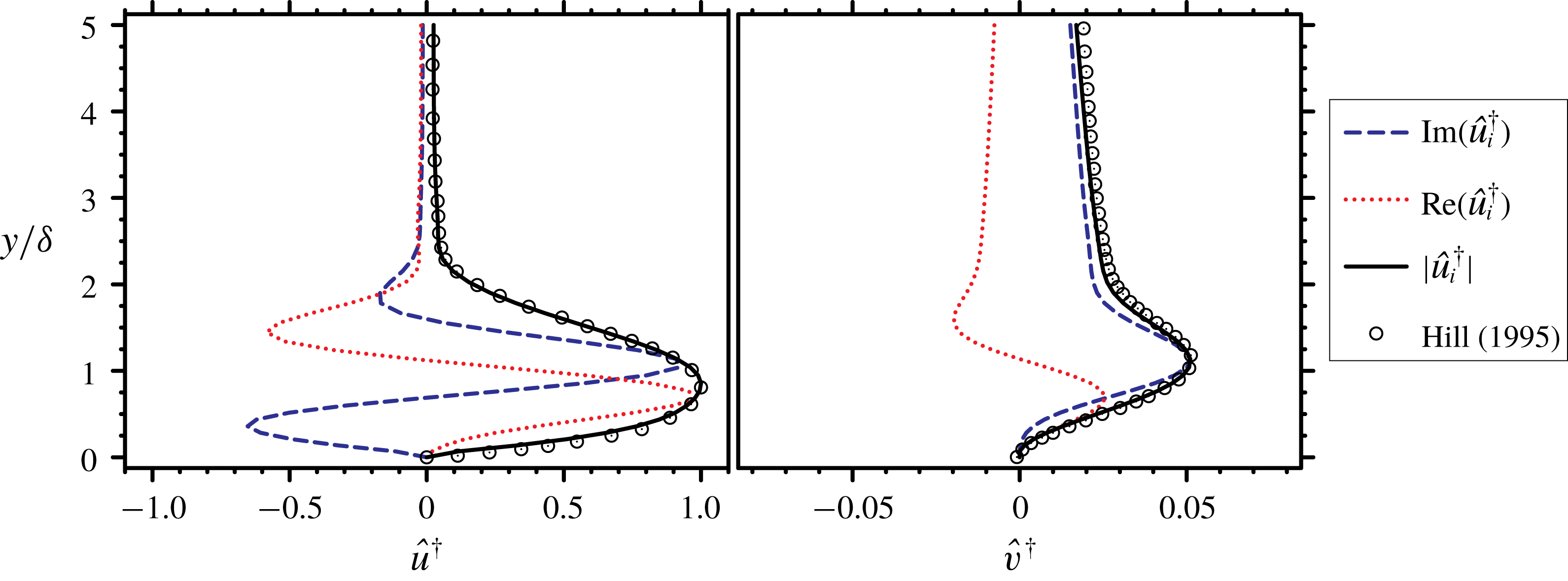
The same time-stepper method is implemented to efficiently compute the leading adjoint eigenvalues and their associated eigenvectors. The solver has been validated for obtaining adjoint modes in appendix A.
2.3.1 Wavemaker
This paper also discusses the receptivity of the JICF to spatially localized feedback. Due to the non-normality of the eigenvalue problem associated with the JICF, adjoint solutions alone cannot describe the whole picture. Therefore, the product for each
 $j$
th pair of direct and adjoint global modes is computed as
 $$\begin{eqnarray}\displaystyle W_{j}(x,y,z)={\displaystyle \frac{\Vert \hat{\boldsymbol{u}}^{j}\Vert \Vert \hat{\boldsymbol{u}}^{\dagger ,j}\Vert }{\text{max}(\Vert \hat{\boldsymbol{u}}^{j}\Vert \Vert \hat{\boldsymbol{u}}^{\dagger ,j}\Vert )}}, & & \displaystyle\end{eqnarray}$$
which determines the region where the eigenvalues of
 $\boldsymbol{A}$
are most sensitive to localized feedback (Giannetti & Luchini Reference Giannetti and Luchini2007) – also called ‘wavemaker’ regions. Locations where
 $W\approx 1$
are sensitive to localized feedback. The value of
 $W$
may be interpreted as a quantification of a possible change in the eigenvalues as a result of applied perturbations in the given region (Ilak et al.
Reference Ilak, Schlatter, Bagheri and Henningson2012). Additionally, Giannetti & Luchini (Reference Giannetti and Luchini2007) have shown that the eigenvalues from linear stability analysis and adjoint sensitivity analysis are sensitive to domain size changes when values of the wavemaker,
 $W_{j}$
, are substantially different from zero at locations close to the domain boundaries. In wavemaker results that follow, all of the isocontours are displayed with a value of
 $0.01$
, and are spatially located far from the edges of the domain.
2.4 Optimal perturbation analysis
Non-modal stability analysis, or optimal perturbation analysis, is widely used in the literature for a variety of problems, as reviewed by Schmid (Reference Schmid2007). The traditional concept of Lyapunov stability does not coincide with non-modal stability analysis. Furthermore, the shape of the eigenmodes from optimal perturbation analysis and traditional asymptotic-time stability analysis can vary significantly, as they describe stability from different perspectives.
The energy is normalized with the initial energy when describing the transient growth
 $$\begin{eqnarray}\displaystyle {\displaystyle \frac{E(\unicode[STIX]{x1D70F})}{E_{0}}}={\displaystyle \frac{(\tilde{\boldsymbol{u}}(\unicode[STIX]{x1D70F}),\tilde{\boldsymbol{u}}(\unicode[STIX]{x1D70F}))}{(\tilde{\boldsymbol{u}}_{0},\tilde{\boldsymbol{u}}_{0})}}, & & \displaystyle\end{eqnarray}$$
where
 $\unicode[STIX]{x1D70F}$
is the time scale over which the transient growth is optimized. This value of
 $\unicode[STIX]{x1D70F}$
is often smaller than the
 $\unicode[STIX]{x1D70F}$
used in linear stability analysis and adjoint sensitivity stability analysis in the previous sections. The perturbation energy may also be expressed in terms of the evolution operators
 $\unicode[STIX]{x1D63D}$
and
 $\unicode[STIX]{x1D63D}^{\dagger }$
defined above:
 $$\begin{eqnarray}\displaystyle {\displaystyle \frac{E(\unicode[STIX]{x1D70F})}{E_{0}}}={\displaystyle \frac{(\unicode[STIX]{x1D63D}\tilde{\boldsymbol{u}}_{0},\unicode[STIX]{x1D63D}\tilde{\boldsymbol{u}}_{0})}{(\tilde{\boldsymbol{u}}_{0},\tilde{\boldsymbol{u}}_{0})}}={\displaystyle \frac{(\tilde{\boldsymbol{u}}_{0},\unicode[STIX]{x1D63D}^{\dagger }\unicode[STIX]{x1D63D}\tilde{\boldsymbol{u}}_{0})}{(\tilde{\boldsymbol{u}}_{0},\tilde{\boldsymbol{u}}_{0})}}. & & \displaystyle\end{eqnarray}$$
We are interested in the initial perturbations,
 $\tilde{\boldsymbol{u}}_{0}$
, that result in the largest transient growth. Equation (2.12) reveals that
 $\tilde{\boldsymbol{u}}_{0}$
is determined by the eigenvalues and eigenmodes of the operator
 $\unicode[STIX]{x1D63D}^{\dagger }\unicode[STIX]{x1D63D}$
. The eigenvalue problem may be expressed as
 $$\begin{eqnarray}\displaystyle \unicode[STIX]{x1D726}\boldsymbol{U}^{\ast }=\unicode[STIX]{x1D63D}^{\dagger }\unicode[STIX]{x1D63D}\boldsymbol{U}^{\ast }, & & \displaystyle\end{eqnarray}$$
where
 $\unicode[STIX]{x1D706}_{j}=\text{diag}(\unicode[STIX]{x1D726})_{j}$
is the
 $j$
th eigenvalue (i.e. growth factor) and
 $\unicode[STIX]{x1D650}^{\ast }=(\boldsymbol{u}^{\ast ,1},\boldsymbol{u}^{\ast ,2},\ldots ,\boldsymbol{u}^{\ast ,N_{\unicode[STIX]{x1D714}}})$
is the matrix of perturbation eigenmodes. The leading eigenmode offers the largest transient growth for the specified value of
 $\unicode[STIX]{x1D70F}$
, but sub-optimal eigenmodes often provide valuable insight towards other flow mechanisms that generate energy growth. In the discussions to follow, sub-optimal eigenmodes (i.e. perturbations) have smaller growth rates, but can become significant to the overall dynamics if their growth rates are near leading growth rate.
The size of the eigenvalue problem associated with optimal perturbation analysis is also computationally expensive to solve. The same method, the IRAM, is used to solve for the leading growth factors and the associated optimal perturbations. However, for optimal perturbation analysis, the eigenvalue problem is already formulated as a time-stepper method. The right-hand side of (2.13) is analogous to integrating a velocity perturbation forward some time
 $\unicode[STIX]{x1D70F}$
through the LNS equations, then backwards for time
 $\unicode[STIX]{x1D70F}$
through the adjoint equations. Therefore, the IRAM solves for the leading eigenvalues and eigenmodes without any further manipulation. This approach has been validated in appendix B.
2.5 Base flow generation
Linear stability, adjoint sensitivity and optimal perturbation analyses require a base flow around which the governing equations are linearized. For increasingly complex and globally unstable flows, obtaining a steady-state solution becomes difficult and computationally expensive. Hence, other approaches are being followed to solve for base flow to study more interesting and complex problems. Selective frequency damping (Åkervik et al. Reference Åkervik, Brandt, Henningson, Hœpffner, Marxen and Schlatter2006) is one such approach to obtain a steady-state solution where a forcing term which acts as a temporal low-pass filter is added to the right-hand side of the governing equations. Some knowledge of the lowest unstable frequency is required for choosing the filter width. In order to converge to a steady solution, the filter cut-off frequency must be lower than that of all of the flow instabilities. Although this method lends itself to easy implementation, the computational cost is governed by the range of time scales. Additionally, selective frequency damping fails to dampen instabilities that are non-oscillatory, as shown by Vyazmina (Reference Vyazmina2010).
Another option is to use a turbulent mean flow as base state. Perhaps the best known example where linear stability analysis about the turbulent mean flow succeeds over the steady-state solution is the oscillating wake of a circular cylinder (Barkley Reference Barkley2006). The solutions about both base states agree at the onset of instability, but the steady-state base flow fails to capture the observed vortex shedding frequency far away from the bifurcation point. Recent studies by Turton, Tuckerman & Barkley (Reference Turton, Tuckerman and Barkley2015) and Tammisola & Juniper (Reference Tammisola and Juniper2016) used turbulent mean flow as a base state to examine linear stability around a turbulent mean flow. Barkley (Reference Barkley2006) and Turton et al. (Reference Turton, Tuckerman and Barkley2015) showed that performing linear stability analysis on a turbulent mean flow as base state results in eigenvalues with small real part and non-zero imaginary part.
Using turbulent mean flow as base state for the present JICF requires further discussion. Since a turbulent mean flow is a solution to the Reynolds-averaged Navier–Stokes equations, a nonlinear Reynolds stress term is effectively added to the governing equations when the base flow equations are used. This translates into a mode-dependent Reynolds stress being present in the eigenvalue problem. A scale-separation argument, first introduced by Crighton & Gaster (Reference Crighton and Gaster1976), and more recently discussed in the review by Jordan & Colonius (Reference Jordan and Colonius2013), can be used to justify when the mode-dependent Reynolds stress term is negligible. Only for the modes of interest (typically low frequency and large scale) must the Reynolds stress term be shown to be unimportant. Regan & Mahesh (Reference Regan and Mahesh2017) demonstrated that
 $St$
computed using the linearization around turbulent mean flow matches the results of DNS of Iyer & Mahesh (Reference Iyer and Mahesh2016). This proves empirically that using a turbulent mean flow as a base state for stability and sensitivity analyses can provide meaningful physical insight into flow dynamics. Additionally, the maximal value of Reynolds shear stress is negligible in the near field for both the mean flow fields (see appendix C), providing further justification for using the turbulent mean flows as base states.
Mantič-Lugo, Arratia & Gallaire (Reference Mantič-Lugo, Arratia and Gallaire2014) proposed a self-consistent model to obtain a base state identical to turbulent mean flow without requiring full nonlinear DNS. Their model requires knowledge of the most unstable mode and the saturation amplitude is determined by requiring the mean flow to be neutrally stable. The model was shown to give excellent results for flow over a circular cylinder compared to DNS in the range
 $50<Re<110$
. Their model, however, may not be directly applicable to a more complex problem such as JICF where the dynamics is dominated by multiple frequencies and
 $Re$
is high.
3 Problem description
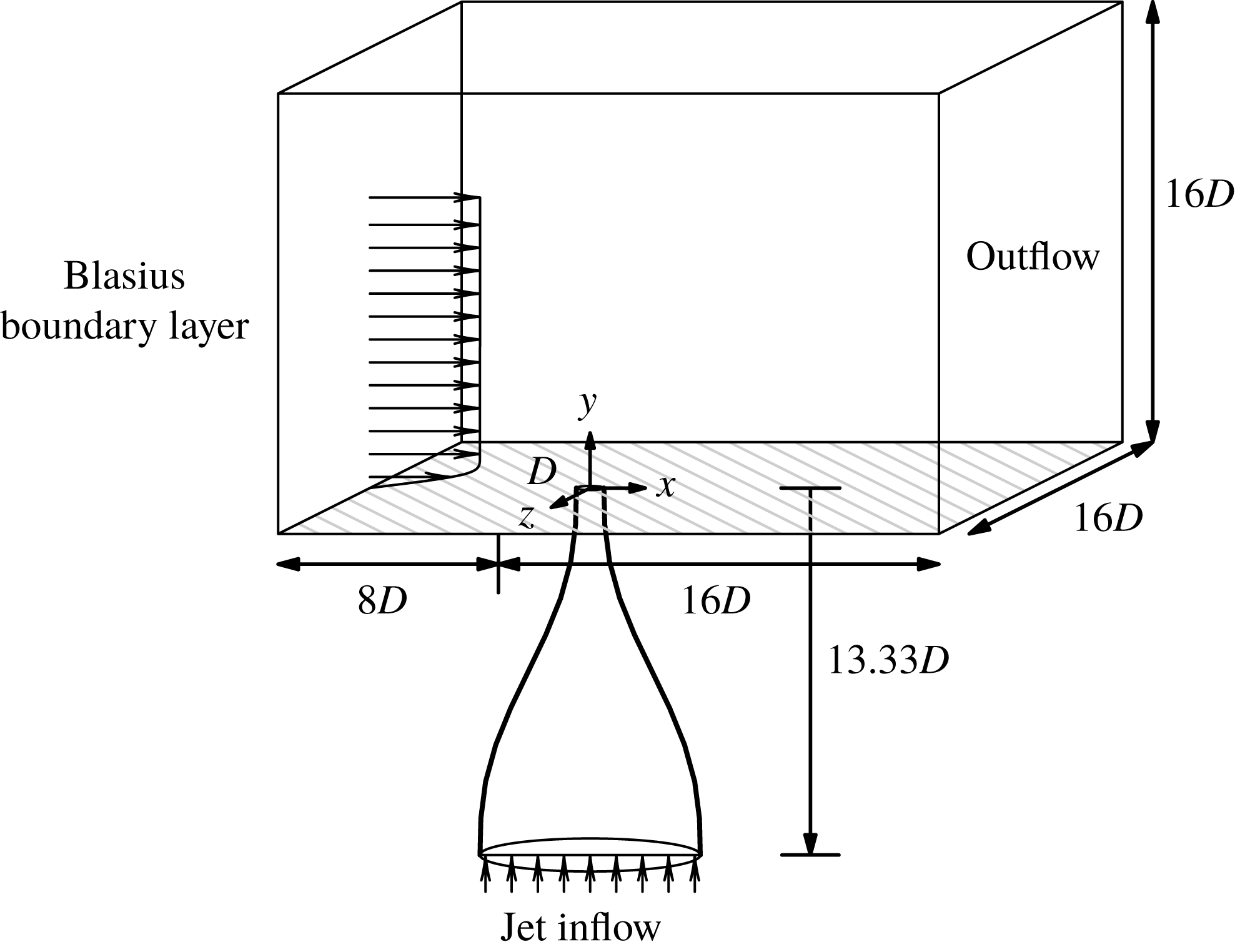
The simulation set-up along with details of the computational domain are shown in figure 2. The domain inflow and outflow boundaries are located
 $8D$
upstream and
 $16D$
downstream of the jet exit, respectively. The lateral boundaries are located at
 $8D$
from the origin in the spanwise direction. The top of the domain is located
 $16D$
above the origin. The jet nozzle is located at the origin of the computational domain and is included in all simulations. It has been shown by Iyer & Mahesh (Reference Iyer and Mahesh2016) that the jet nozzle plays a crucial role in setting up the mean flow near the jet exit, thus affecting the stability characteristics of the flow. A fifth-order polynomial is used to model the nozzle shape used in the experiments of Megerian et al. (Reference Megerian, Davitian, Alves and Karagozian2007). The jet exit diameter
 $D$
is
 $3.81~\text{mm}$
and the average velocity at the jet exit
 $\overline{v}_{jet}$
is
 $8~\text{m}~\text{s}^{-1}$
. The simulated nozzle extends
 $13.33D$
below the jet orifice.
Schematic of the problem set-up showing the computational domain.

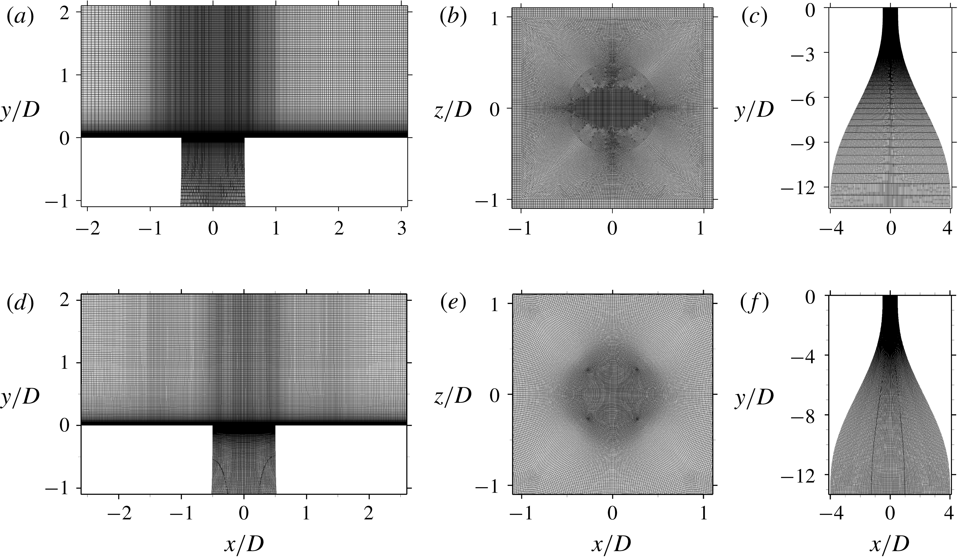
A view of the symmetry plane (a,d), a wall-normal plane near the jet exit (b,e) and the nozzle (c,f) are shown for the 80-million-element (a–c) and the 138-million-element (d–f) grids.

Simulation details for GLSA and GASA. An alternative cross-flow ratio,
 $R^{\ast }$
, is shown based on the jet exit peak velocity
 $v_{jet,max}$
. The momentum thickness (
 $\unicode[STIX]{x1D703}_{bl}$
) of the cross-flow boundary layer is described at the jet exit when the jet is off.

A laminar Blasius boundary layer is prescribed at the inflow. The physical parameters, the computational domain and the cross-flow boundary layer are identical to those used by Iyer & Mahesh (Reference Iyer and Mahesh2016), who showed the boundary layer to match well with the experiments of Megerian et al. (Reference Megerian, Davitian, Alves and Karagozian2007) at
 $x/D=-5.5$
. Neumann boundary conditions are applied to the lateral and top boundaries. A uniform inflow velocity is prescribed at the nozzle inflow to achieve the desired velocity at the jet exit. Simulation cases
 $R2$
and
 $R4$
are performed under the same conditions as in the experiments of Megerian et al. (Reference Megerian, Davitian, Alves and Karagozian2007). Additional simulation details are outlined in table 1.
The computational grids are shown in figure 3, and are made up of 80 million and 138 million elements, respectively. The 80-million-element grid has 80 elements inside the inflow laminar boundary layer in the wall-normal direction and 400 elements around the jet exit. The grid spacings are
 $\unicode[STIX]{x0394}x/D=0.033$
and
 $\unicode[STIX]{x0394}z/D=0.02$
, with
 $\unicode[STIX]{x0394}y_{min}/D=0.0013$
downstream of the jet exit, which are finer than used by Muppidi & Mahesh (Reference Muppidi and Mahesh2007) to simulate a turbulent JICF. Assuming the boundary layer downstream of the jet exit to be turbulent, grid resolution can be computed in viscous units (e.g.
 $\unicode[STIX]{x0394}x^{+}=\unicode[STIX]{x0394}xu_{\unicode[STIX]{x1D70F}}/\unicode[STIX]{x1D708}$
), where the local wall shear stress (
 $\unicode[STIX]{x1D70F}_{w}$
) is used to calculate the friction velocity
 $u_{\unicode[STIX]{x1D70F}}=\sqrt{\unicode[STIX]{x1D70F}_{w}/\unicode[STIX]{x1D70C}}$
. Wall spacings (
 $\unicode[STIX]{x0394}x^{+}$
,
 $\unicode[STIX]{x0394}y_{min}^{+}$
,
 $\unicode[STIX]{x0394}z^{+}$
) near the outflow are (
 $2.74$
,
 $0.1$
,
 $1.66$
) and (
 $1.48$
,
 $0.058$
,
 $0.89$
) for case
 $R2$
and case
 $R44$
, respectively.
For the 138-million-element grid, 86 elements are inside of the inflow laminar boundary layer and 320 elements are around the jet exit. Additionally, downstream of the jet nozzle exit, grid spacings of
 $\unicode[STIX]{x0394}x/D=0.029$
and
 $\unicode[STIX]{x0394}z/D=0.02$
, with
 $\unicode[STIX]{x0394}y_{min}/D=0.0013$
are maintained. Compared to the 80-million-element grid, this grid is refined in the jet nozzle and cross-flow boundary layer. Grid resolutions in terms of wall units are
 $\unicode[STIX]{x0394}x^{+}=2.10$
,
 $\unicode[STIX]{x0394}y_{min}^{+}=0.09$
and
 $\unicode[STIX]{x0394}z^{+}=1.45$
for case
 $R2$
and
 $\unicode[STIX]{x0394}x^{+}=1.09$
,
 $\unicode[STIX]{x0394}y_{min}^{+}=0.05$
and
 $\unicode[STIX]{x0394}z^{+}=0.75$
for case
 $R4$
.
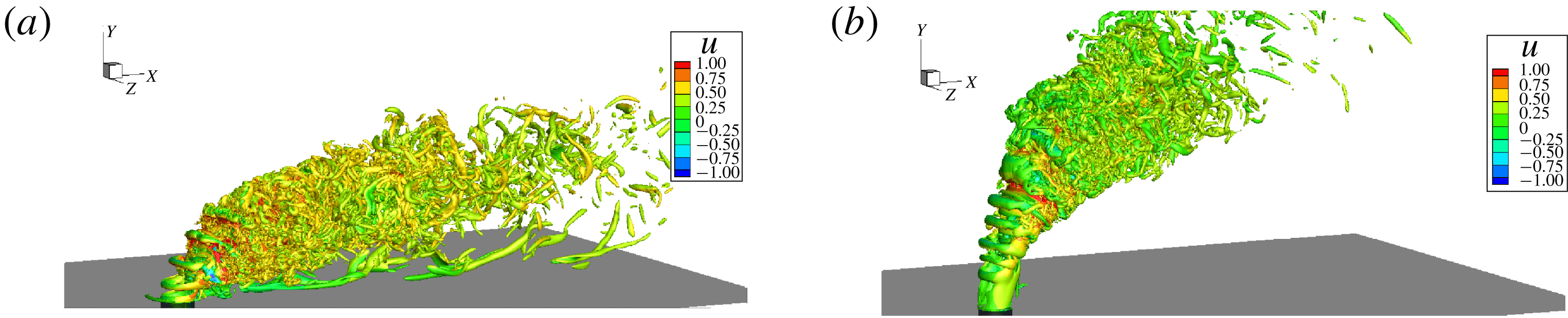
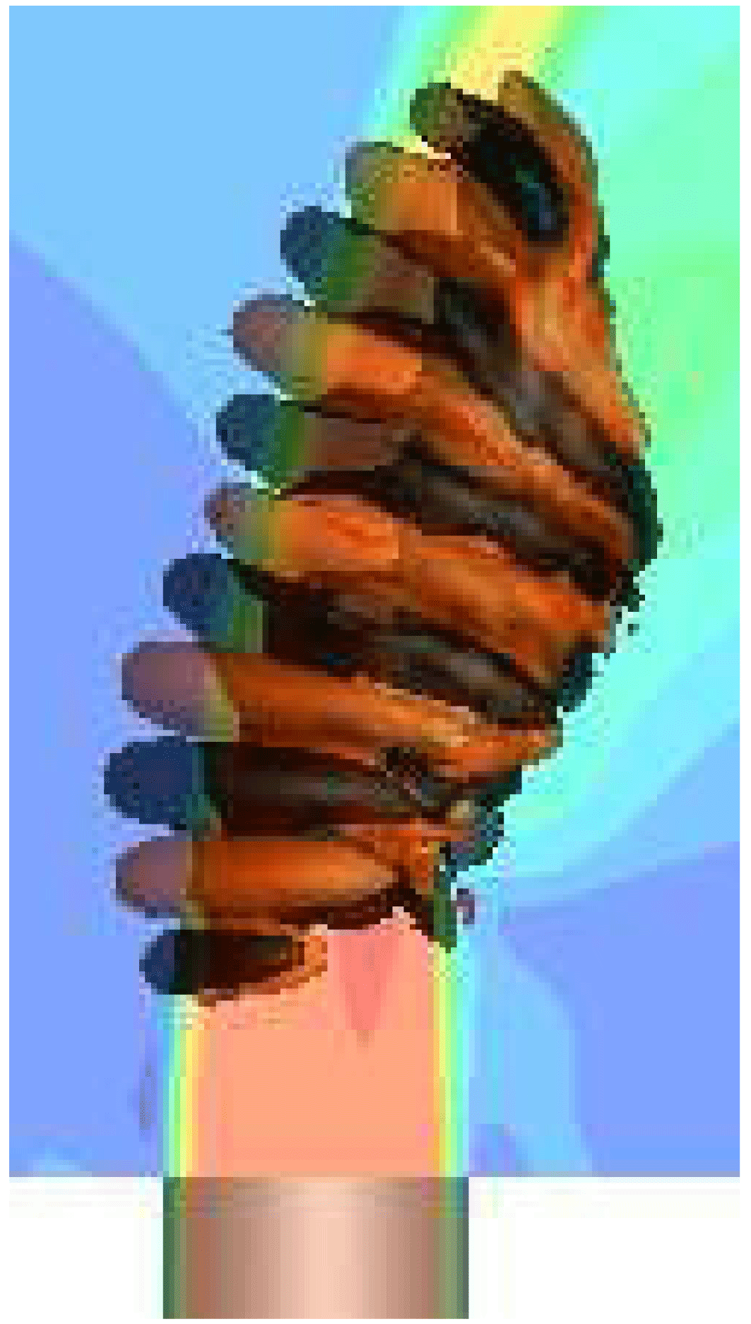
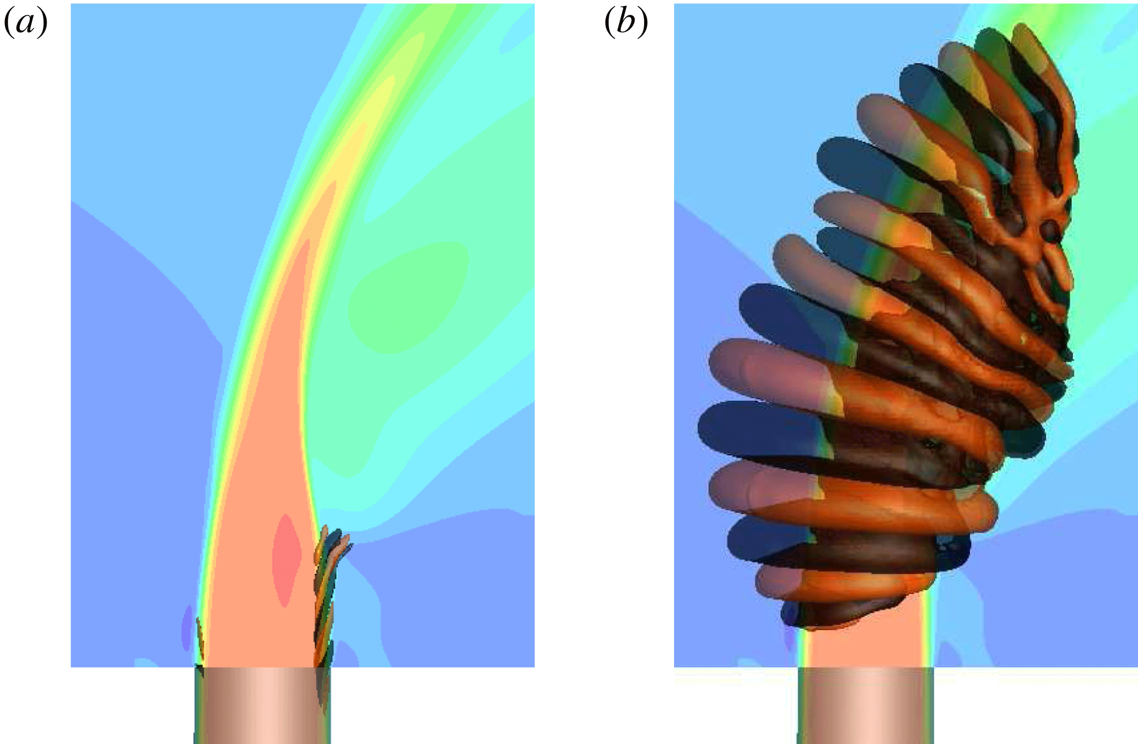
Instantaneous flow fields are shown using isocontours of
 $Q$
-criterion (Hunt et al.
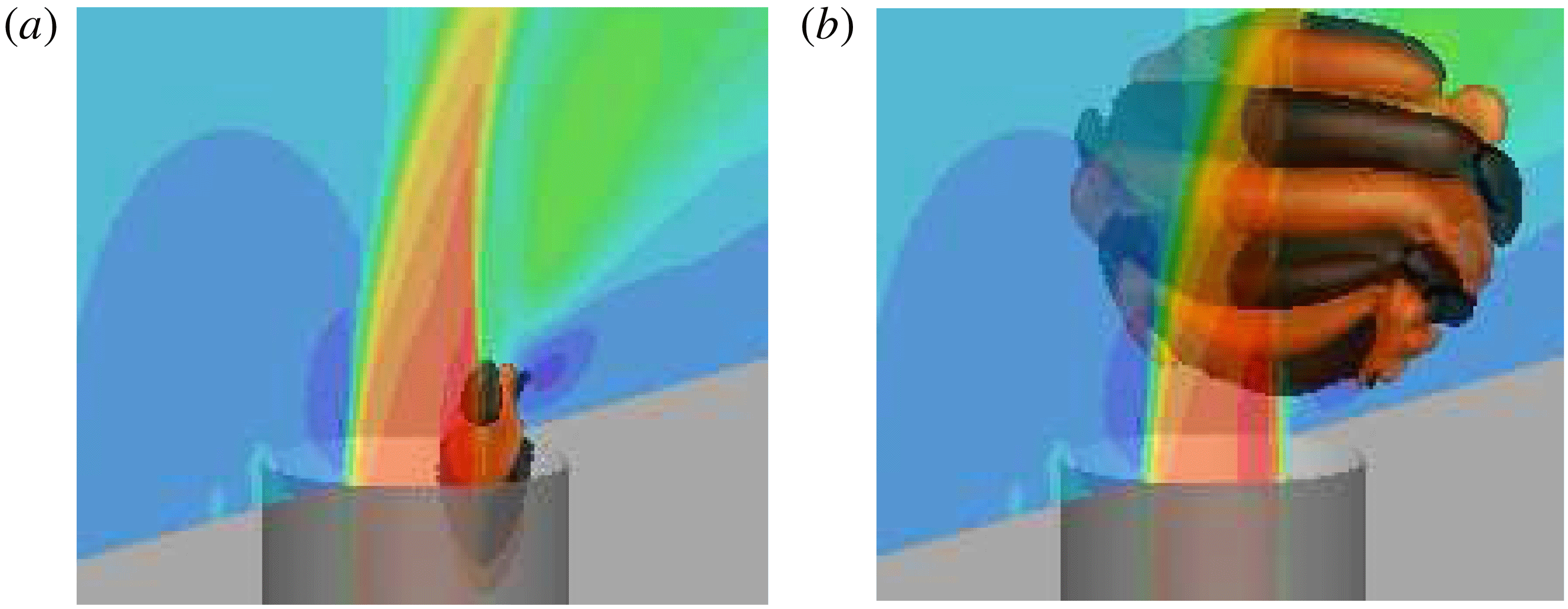
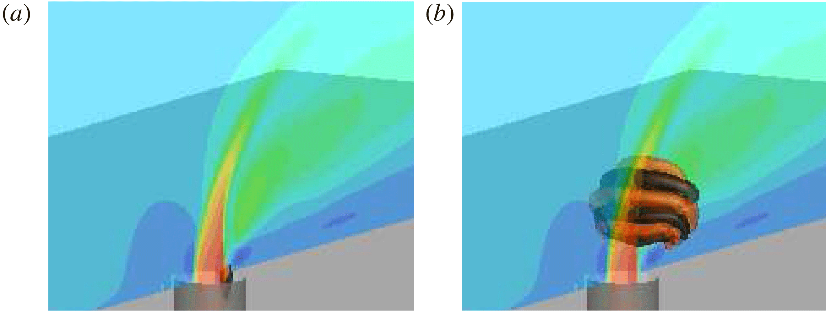
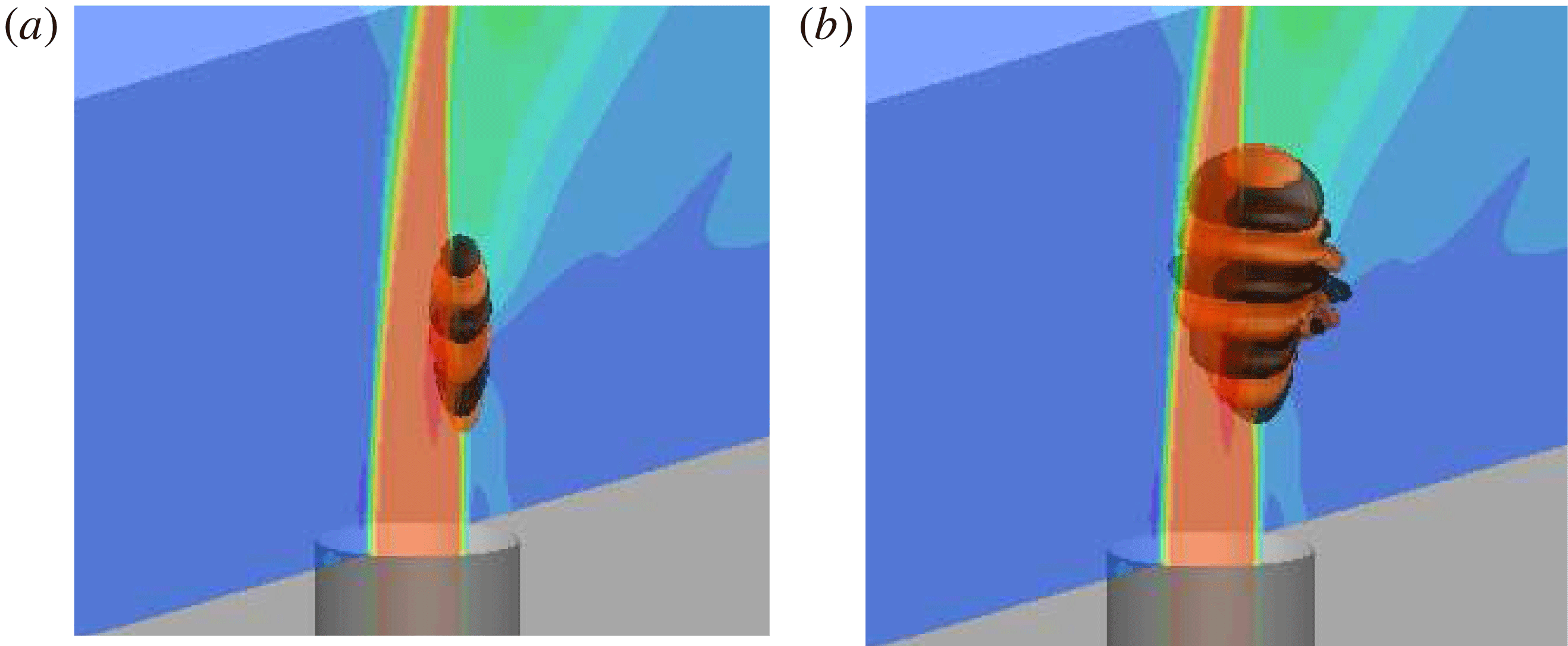
Reference Hunt, Wray and Moin1988) coloured by streamwise velocity in figure 4, which illustrates the complexity of the flow field of the JICF. Important features include the coherent upstream shear-layer roll-up, and long string-like wake vortices near the wall. Additionally, downstream shear-layer roll-up is seen that interacts with the upstream shear layer at the collapse of the potential core. Many fine-scale turbulent flow structures are also visible downstream in the jet wake.
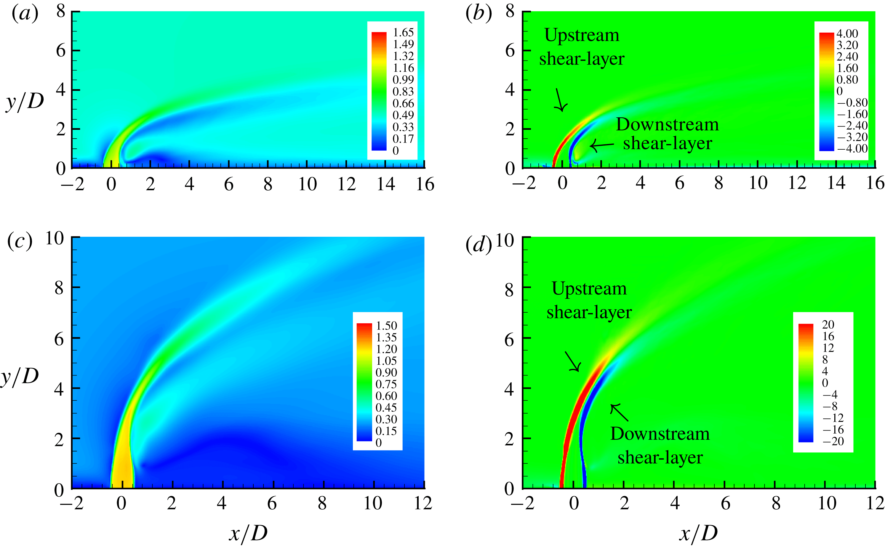
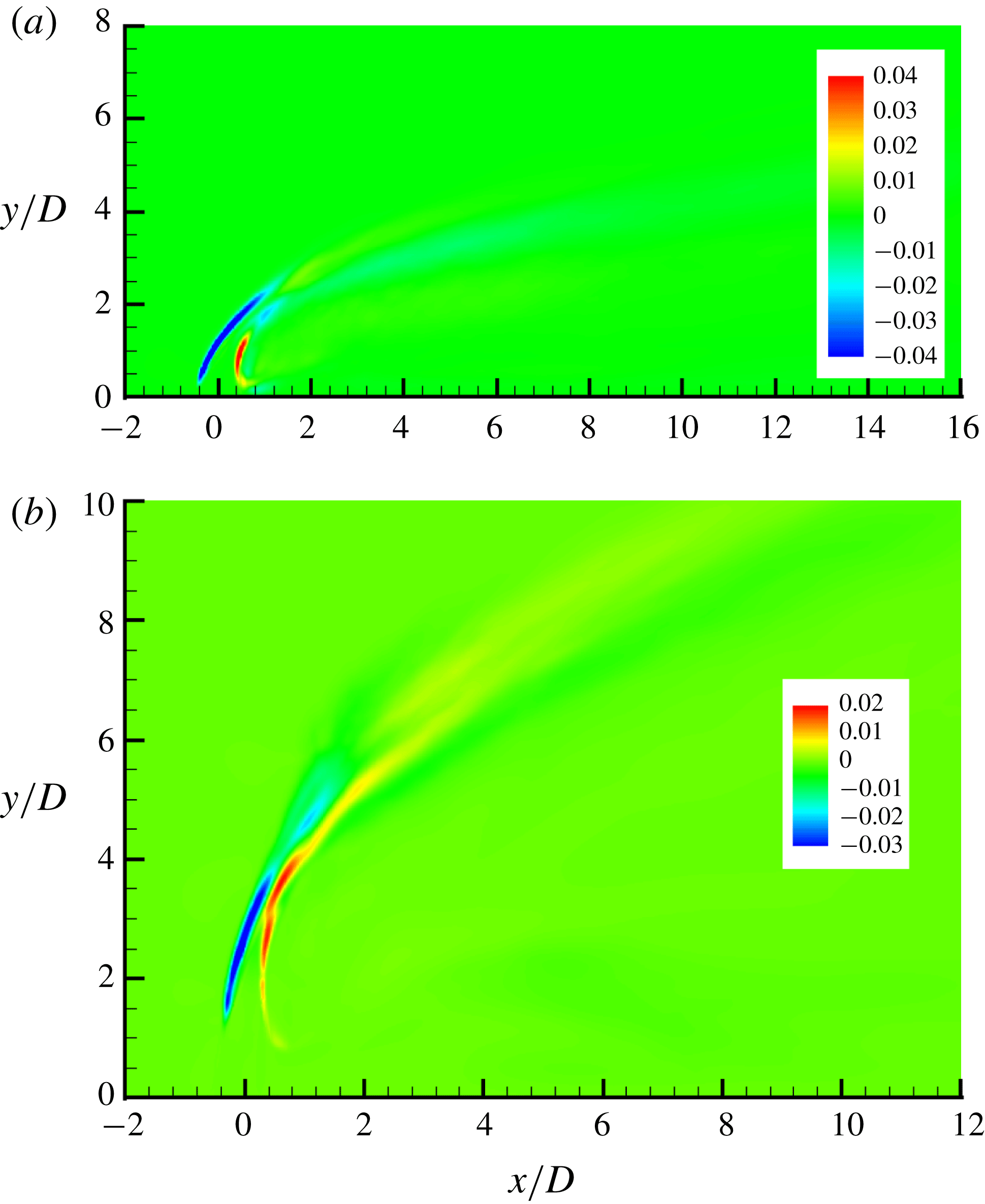
The turbulent flow is time-averaged for both cases to obtain mean flow field (base state). The contours of velocity magnitude and spanwise vorticity are shown in figure 5 for both cases. Except for parts of § 4, results using the
 $138$
-million-element grid are reported. The turbulent mean flows for the
 $80$
-million-element grid were generated by Iyer & Mahesh (Reference Iyer and Mahesh2016) using
 $32\,000$
and
 $39\,000$
temporal samples for case
 $R2$
and
 $R4$
, respectively. Iyer & Mahesh (Reference Iyer and Mahesh2016) have shown that there is good agreement between the temporally averaged solutions from simulation and experiment. Similarly, for the
 $138$
-million-element grid,
 $54\,000$
and
 $70\,000$
samples are used for cases
 $R2$
and
 $R4$
, respectively. The non-dimensionalized time difference between two successive instantaneous samples
 $\unicode[STIX]{x0394}t=tv_{jet,max}/D\approx 8\times 10^{-4}$
for both cases and both grids.
Isocontour of
 $Q$
-criterion coloured by streamwise velocity for the instantaneous turbulent flow field for
 $R=2$
(a) and
 $R=4$
(b).

The contours of velocity magnitude (a,c) and spanwise vorticity (b,d) are shown for the base flows for
 $R2$
(a,b) and
 $R4$
(c,d) cases in the symmetry plane.

4 Direct and adjoint analyses of the JICF
This section presents results from linear stability and adjoint sensitivity analysis of cases
 $R2$
and
 $R4$
. The behaviours in the upstream shear layer, CVP, downstream of the jet exit and downstream shear layer are all discussed. All linear stability and adjoint sensitivity results were converged to a maximum residual of
 $1\times 10^{-14}$
while using
 $100$
Arnoldi vectors. For case
 $R2$
,
 $18$
leading eigenvalues are computed. The integration time
 $\unicode[STIX]{x1D70F}$
is
 $0.114$
time units (non-dimensionalized by
 $D/v_{jet,max}$
), to allow for adequate temporal resolution to resolve the highest frequencies in the upstream shear layer from DNS (
 $St_{1}=fD/v_{jet,max}=0.65$
). The low-frequency linear stability results were the focus of the
 $138$
-million-element grid. For linear stability of
 $R4$
, the
 $8$
leading low-frequency eigenmodes were computed using
 $\unicode[STIX]{x1D70F}=0.32$
. Adjoint sensitivity for case
 $R4$
computed the
 $14$
leading eigenvalues. Since the frequencies were already known from linear stability, adjoint sensitivity uses a smaller
 $\unicode[STIX]{x1D70F}=0.16$
, allowing it to capture both the high- and low-frequency eigenvalues.
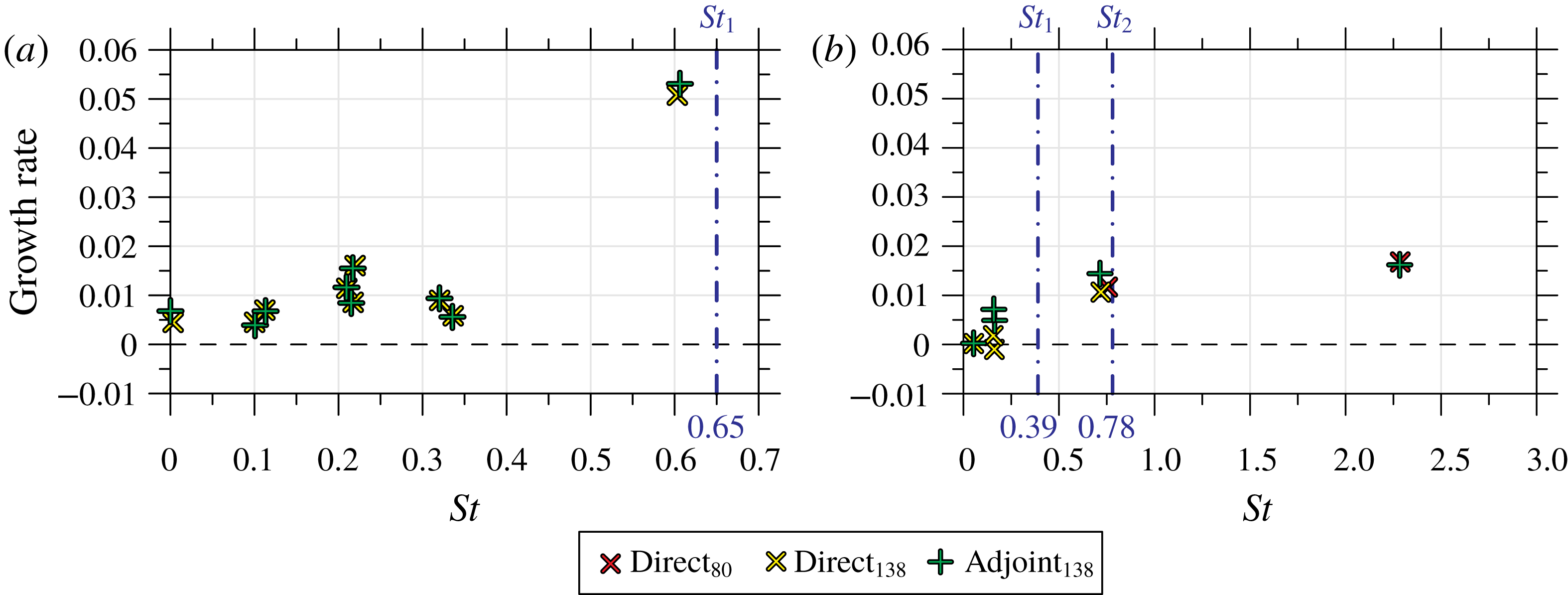
Non-dimensional eigenvalues,
 $\unicode[STIX]{x1D714}^{\ast }$
, from linear stability and adjoint sensitivity for
 $R2$
(a) and
 $R4$
(b). The blue dash-dotted lines correspond to the dominant frequencies observed within the upstream shear layer by Iyer & Mahesh (Reference Iyer and Mahesh2016). The legend subscripts refer to results from the
 $80$
-million-element and
 $138$
-million-element grids.

Figure 6 shows the eigenvalues from the analyses. The complex eigenvalues are non-dimensionalized as
 $\unicode[STIX]{x1D714}^{\ast }$
so the imaginary part is
 $St$
:
 $$\begin{eqnarray}\displaystyle \unicode[STIX]{x1D714}^{\ast }={\displaystyle \frac{\unicode[STIX]{x1D714}D}{2\unicode[STIX]{x03C0}v_{jet,max}}}. & & \displaystyle\end{eqnarray}$$
The direct and adjoint eigenvalues match, and show good agreement with the upstream shear-layer spectra results (i.e. vertical blue dash-dotted lines in figure 6 a,b) from experiments (Megerian et al. Reference Megerian, Davitian, Alves and Karagozian2007) and simulations (Iyer & Mahesh Reference Iyer and Mahesh2016). This implies that the linear assumptions that are used in the analyses herein are valid when considering the stability and sensitivity of the JICF that is temporally averaged to obtain a base flow at these conditions.
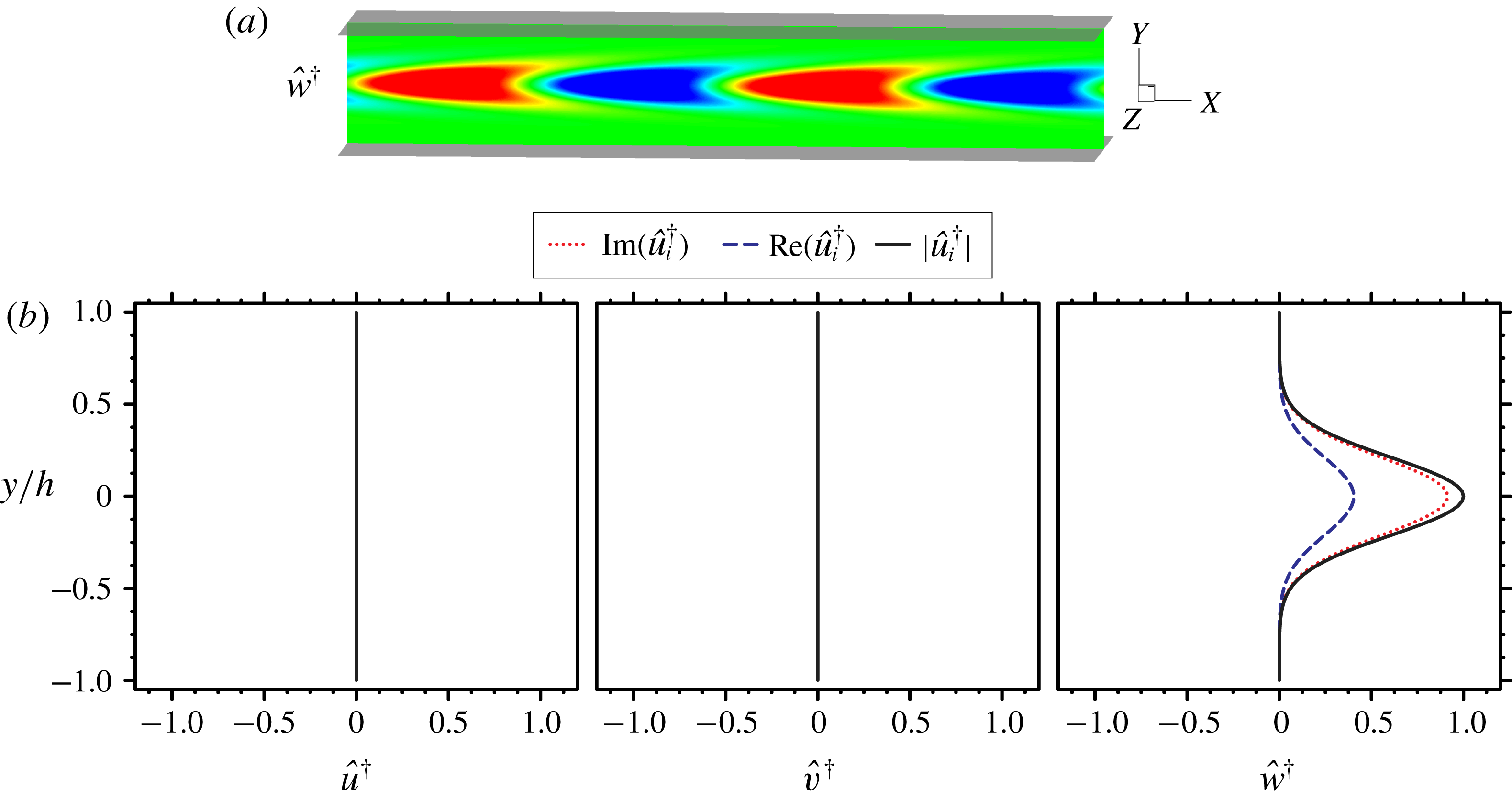
In this section, modes from linear stability analysis are shown using isocontours of the streamwise (
 $x$
-direction) perturbation velocity,
 $Re(\hat{u} )=\pm 0.0003$
. Adjoint sensitivity analysis modes are presented using isocontours of the vertical (
 $y$
-direction) adjoint perturbation velocity,
 $Re(\hat{v}^{\dagger })=\pm 0.0001$
, which highlight regions most sensitive to vertical point momentum forcing. Eigenmodes are normalized such that
 $\Vert \hat{\boldsymbol{u}}\Vert =\Vert \hat{\boldsymbol{u}}^{\dagger }\Vert =1$
.
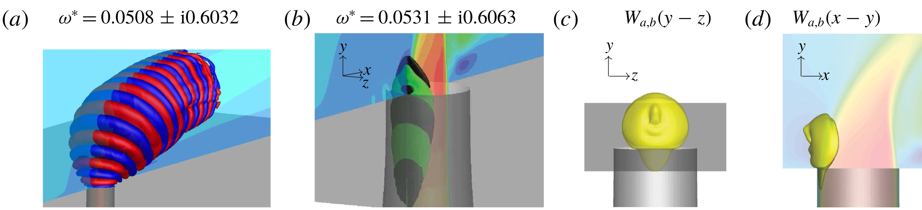
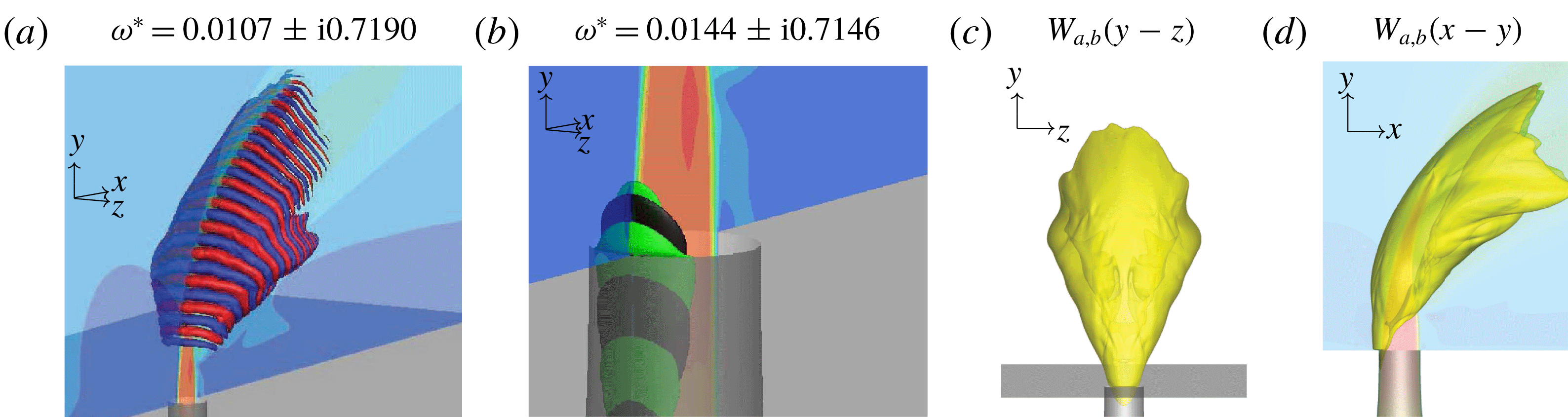
4.1 Upstream shear layer
The upstream shear-layer linear stability eigenmodes for both case
 $R2$
(figure 7
a) and case
 $R4$
(figure 8
a) were discussed in detail by Regan & Mahesh (Reference Regan and Mahesh2017). The main difference between the direct modes for each case is that for case
 $R2$
the mode originates near the jet exit plane, whereas for
 $R4$
the mode is elevated.
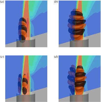
The
 $R2$
upstream shear-layer linear stability (a) and adjoint sensitivity analyses (b) eigenmodes along with their associated wavemaker (c,d). Symmetry plane contours show the vertical velocity of the base flow
 $\overline{v}$
.

Similar to figure 7, but for the
 $R4$
upstream shear layer.

The adjoint eigenmodes (figures 7
b and 8
b) show that the direct modes are most sensitive to
 $y$
-direction momentum forcing along the upstream side of the jet nozzle, near the jet exit. Interestingly, for
 $R2$
the wavemaker region (figure 7
c,d) is localized along the upstream side of the nozzle. Conversely,
 $R4$
(figure 8
c,d) is most sensitive to localized feedback along the entire upstream shear layer.
The wavemaker results are consistent with the notion that the upstream shear-layer region transitions from absolute to convective instability as
 $R$
changes from
 $2$
to
 $4$
. For
 $R2$
, the region most sensitive to localized feedback is dominated by the formation of the upstream shear layer, which is in direct contrast to case
 $R4$
, which is sensitive to localized feedback along the entire upstream shear layer. The tonal nature of case
 $R2$
is due to the fact that the location where the shear layer begins to roll up (and its frequency dominates) is in the same location where the ‘wavemaker’ is the strongest. Case
 $R4$
is not only weaker, but the wavemaker region extends along the upstream shear layer.
4.2 Asymmetries in the CVP
Smith & Mungal (Reference Smith and Mungal1998) observed in their JICF experiments that asymmetries may form in the time-averaged CVP for
 $R>10$
. Similar observations were made by Getsinger et al. (Reference Getsinger, Gevorkyan, Smith and Karagozian2014) in their experiments who concluded that an absolutely unstable JICF (
 $R2$
) is less likely to exhibit asymmetric mean profiles compared to the weaker, convectively unstable JICF (
 $R4$
). The reason behind this behaviour of the JICF is not fully understood; specifically, the reason behind why there is a preferential direction in certain configurations.
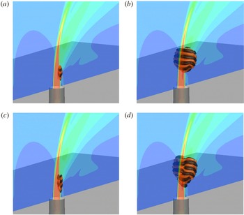
Similar to figure 7, but for the
 $R2$
left-leaning asymmetric eigenmodes. However, the linear stability mode (a) is highlighted using isocontour levels of
 $\pm 0.0001$
to highlight the streaks in the CVP.

Similar to figure 7, but for the
 $R2$
right-leaning asymmetric eigenmodes. However, the linear stability mode (a) is highlighted using isocontour levels of
 $\pm 0.0001$
to highlight the streaks in the CVP.

Similar to figure 7, but for the
 $R4$
left-leaning asymmetric eigenmodes.

Similar to figure 7, but for the
 $R4$
right-leaning asymmetric eigenmodes.

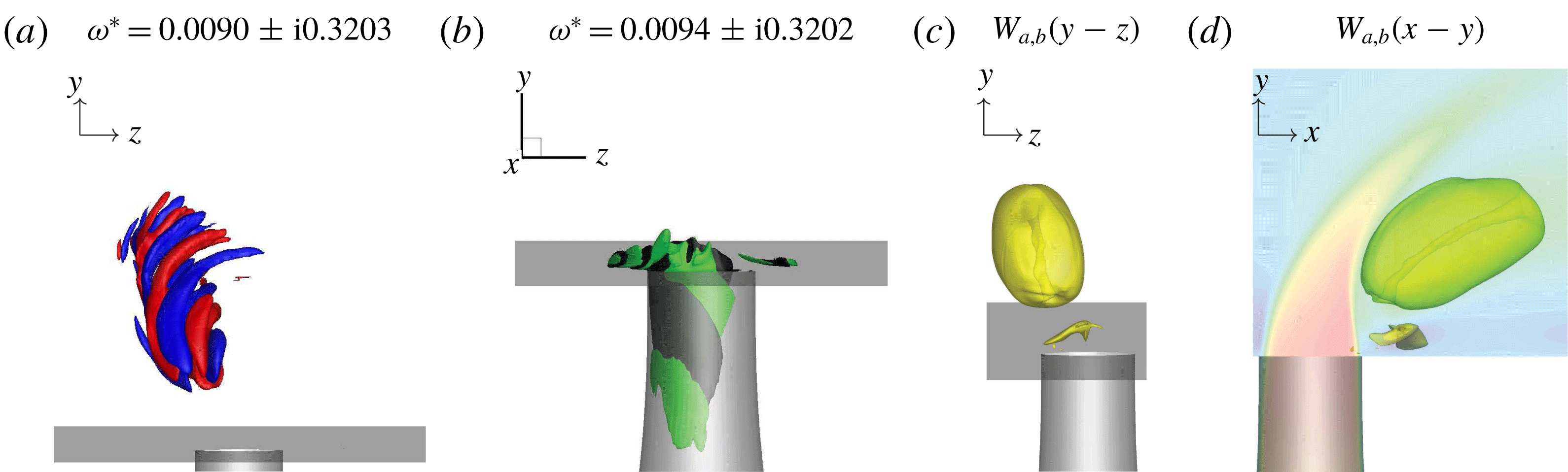
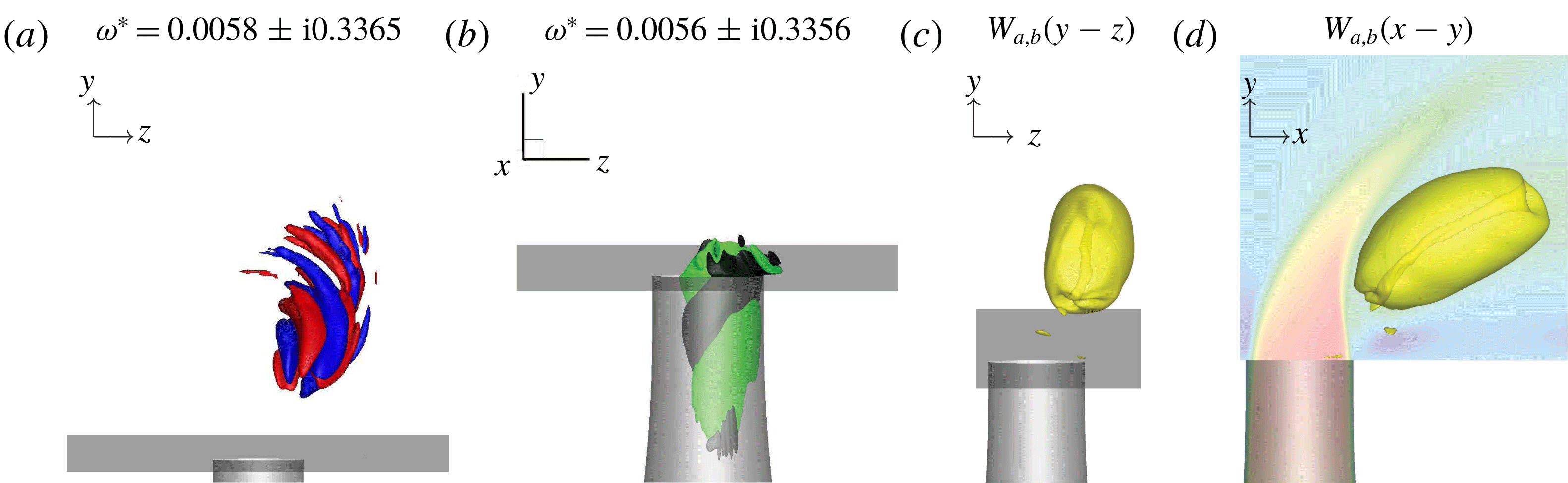
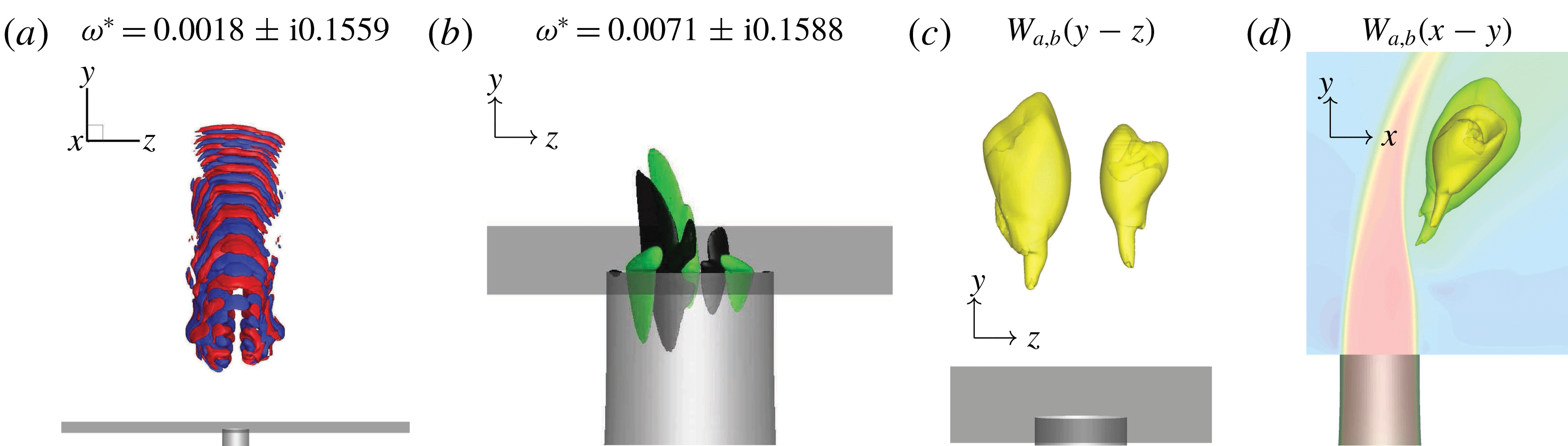
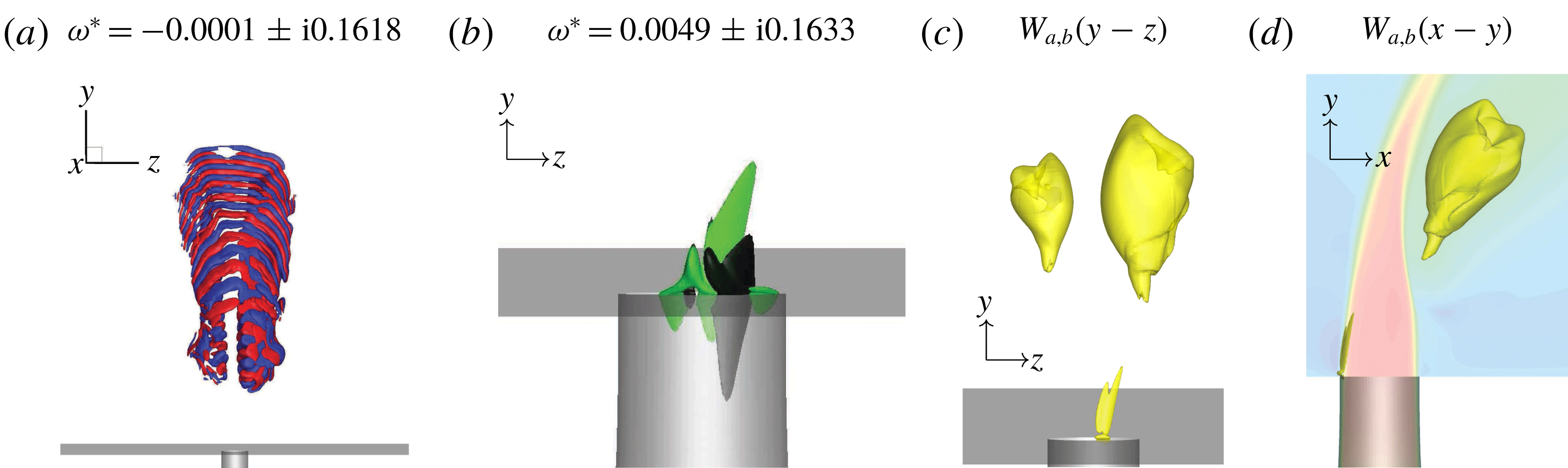
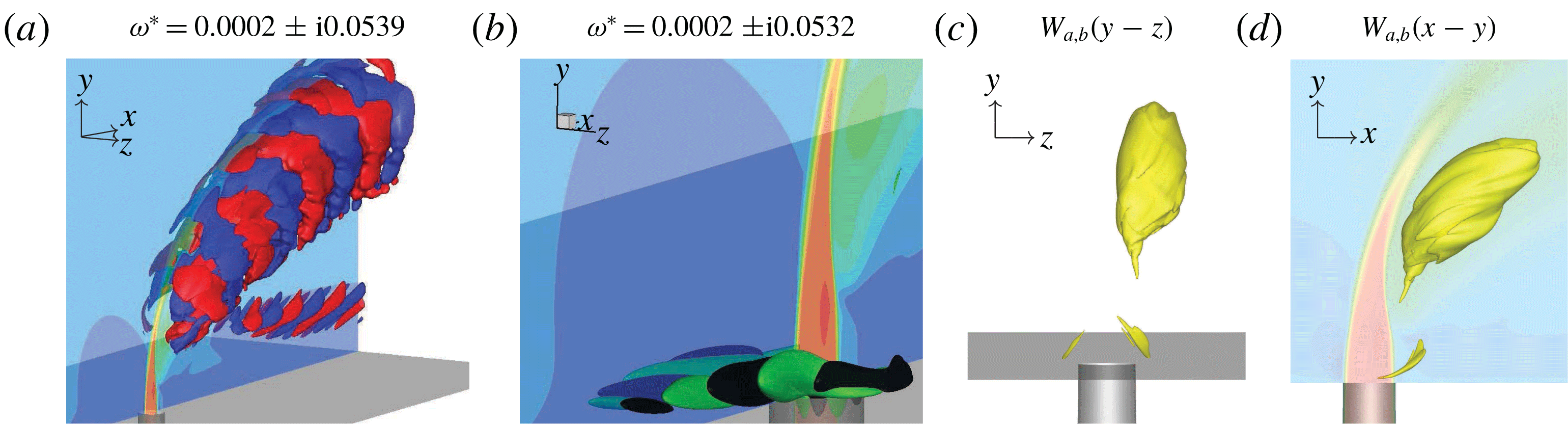
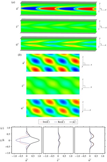
In the present work, we observe significant asymmetries in some eigenmodes. The direct (a) and adjoint (b) eigenmodes in figures 9 and 10 for case
 $R2$
, and figures 11 and 12 for case
 $R4$
are left-leaning and right-leaning, respectively. Their corresponding wavemaker regions are biased towards each side as well. The adjoint eigenmodes (b) are most sensitive to vertical point momentum forcing in a similar way to the upstream shear layers, but with biases to each side. The wavemakers (c,d) are located along the CVP, directly behind the collapse of the jet potential core. By animating the linear stability analysis eigenmodes (not shown) it is seen that the eigenmodes for both cases rotate with the CVP.
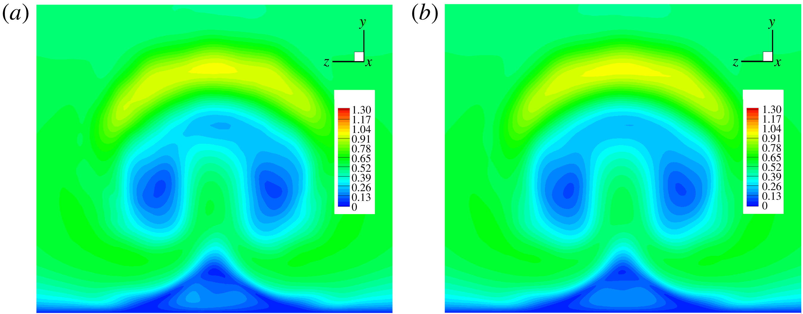
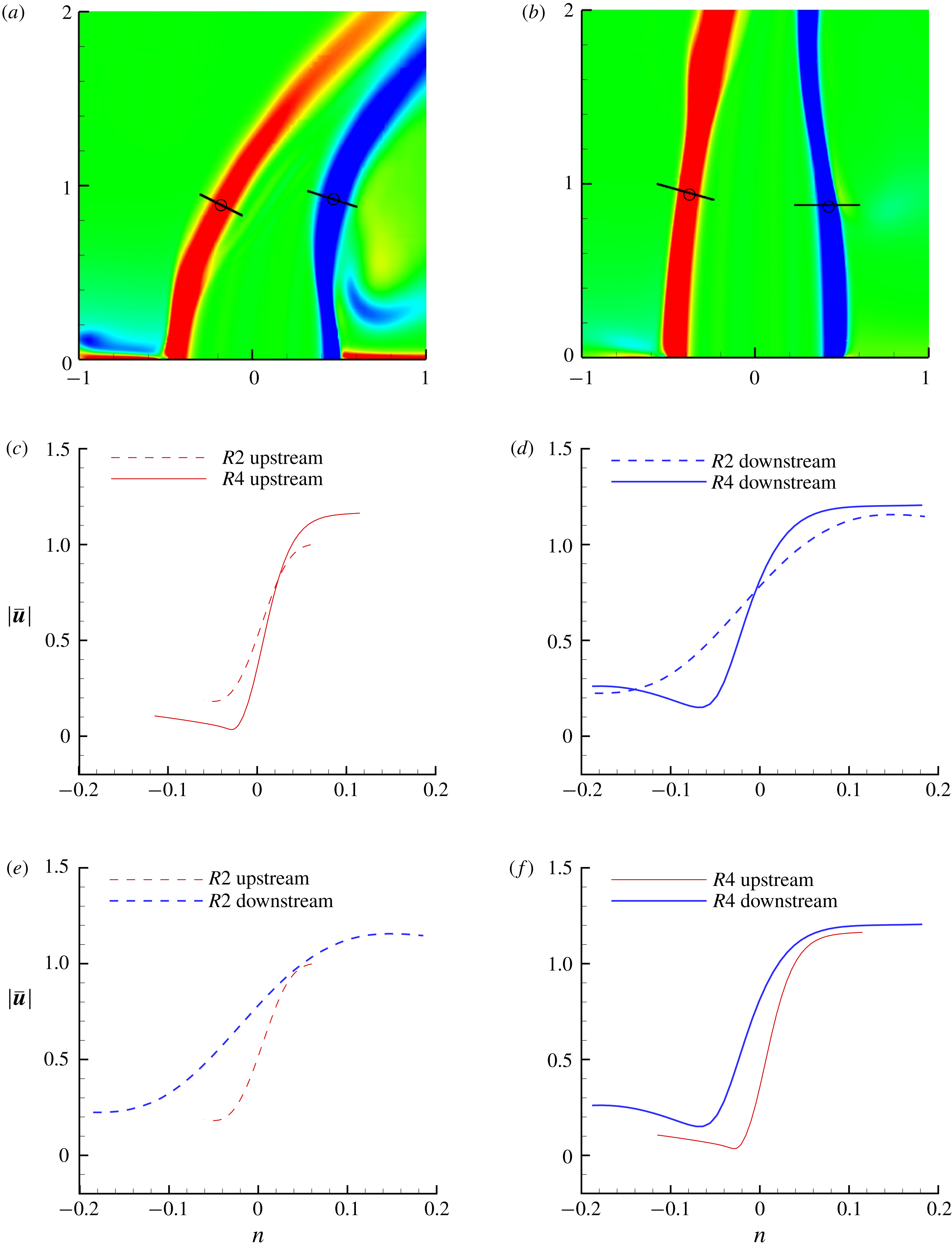
It is important to examine if there are asymmetries present in the turbulent mean flow that are causing asymmetric eigenmodes. For case
 $R2$
, the turbulent mean flow was extended to an average over
 $170\,000$
samples. A contour plot of a
 $yz$
-plane at
 $x=1.33D$
is shown in figure 13 for the original base flow (figure 13
a) and the extended base flow (figure 13
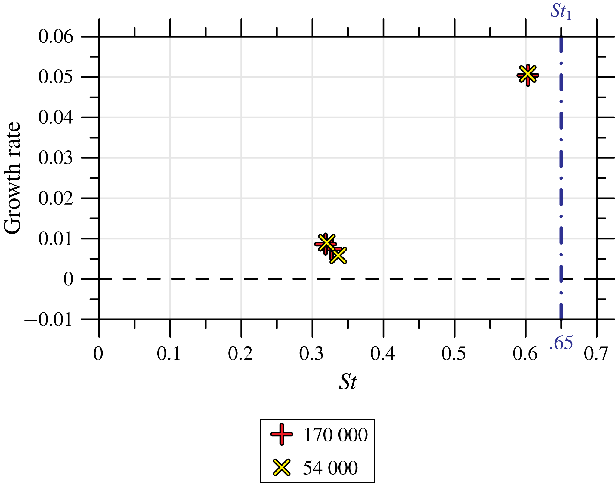
b). Some small differences are visible between the two mean flows near the wall and in the middle of the CVP. Linear stability analysis was performed using the extended base flow, and the results are shown in figure 14. The eigenvalues from both simulations agree very well in both growth rate and
 $St$
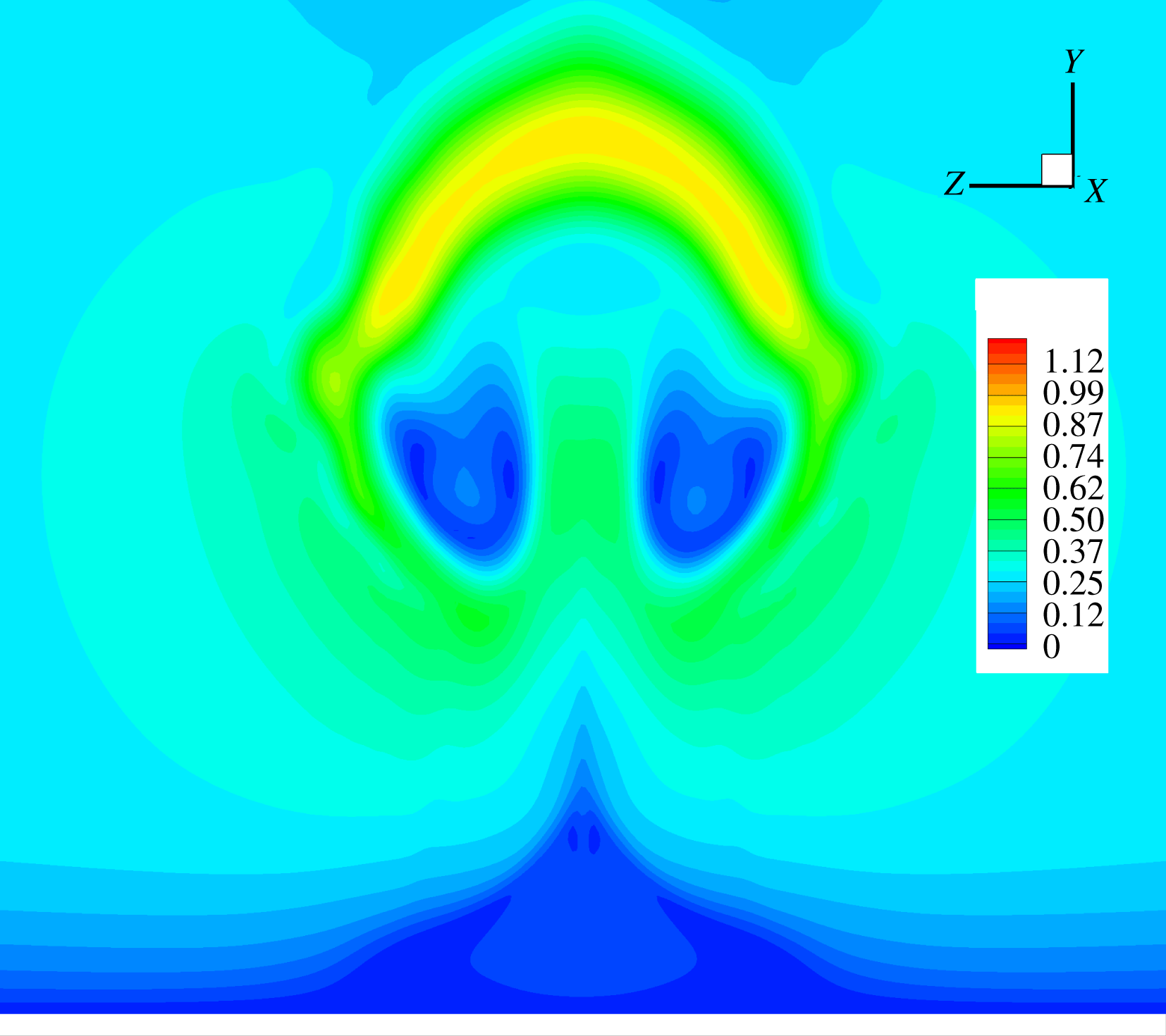
. This provides evidence that the asymmetric eigenmodes are not a construct of an asymmetric mean flow. The turbulent mean flow for case
 $R4$
is also shown in figure 15 using contours on the
 $yz$
-plane at
 $x=D$
. The mean flow for case
 $R4$
does not suffer from asymmetries, and therefore does not require an extended statistics calculation for comparison.
The velocity magnitude of two turbulent mean flows is shown in the
 $yz$
-plane at
 $x=1.33D$
. The first base flow (a) used 54 000 turbulent flow field samples, whereas the second (b) used 170 000 samples.

Comparison of asymmetric mode eigenvalues after additional statistic samples. The upstream shear-layer eigenvalue is also shown for both calculations to provide context.

The velocity magnitude of turbulent mean flow is shown in the
 $yz$
-plane at
 $x=D$
.

Linear stability analysis results for case
 $R2$
originate much closer to the jet nozzle exit compared to case
 $R4$
. The adjoint modes provide valuable information regarding the sensitivity of these asymmetric instabilities to
 $y$
-direction point momentum forcing. Note the spatial and temporal length scales that characterize the regions where asymmetric instabilities are most sensitive. For instance, adjoint sensitivity analysis results for case
 $R2$
(figure 9
b) show much longer length scales in the circumferential direction just below the jet nozzle exit when compared to case
 $R4$
(figure 11
b). This knowledge, in conjunction with the frequency information, provides valuable information regarding the best location and frequencies to excite asymmetries.
Growth rates from the linear stability and adjoint sensitivity analyses are often discussed in terms of their relative strength. We can compute the relative strength of the asymmetric eigenmodes for each case by comparing them to the strength of their respective upstream shear-layer growth rates. The difference
 $\unicode[STIX]{x0394}\unicode[STIX]{x1D714}_{R2}^{\ast }$
between the growth rates of asymmetric eigenmodes and the upstream shear-layer eigenmodes for case
 $R2$
is in the range
 $0.042\leqslant \unicode[STIX]{x0394}\unicode[STIX]{x1D714}_{R2}^{\ast }\leqslant 0.047$
. However, for the
 $R4$
case, the difference
 $\unicode[STIX]{x0394}\unicode[STIX]{x1D714}_{R4}^{\ast }$
is in the range
 $0.014\leqslant \unicode[STIX]{x0394}\unicode[STIX]{x1D714}_{R4}^{\ast }\leqslant 0.009$
. Notice
 $\unicode[STIX]{x0394}\unicode[STIX]{x1D714}_{R2}^{\ast }>\unicode[STIX]{x0394}\unicode[STIX]{x1D714}_{R4}^{\ast }$
over their entire ranges, suggesting that asymmetric modes and sensitivity to experimental asymmetries are more significant for
 $R4$
than
 $R2$
, consistent with experimental results (Smith & Mungal Reference Smith and Mungal1998; Getsinger et al.
Reference Getsinger, Gevorkyan, Smith and Karagozian2014).
4.3 Downstream of the jet exit
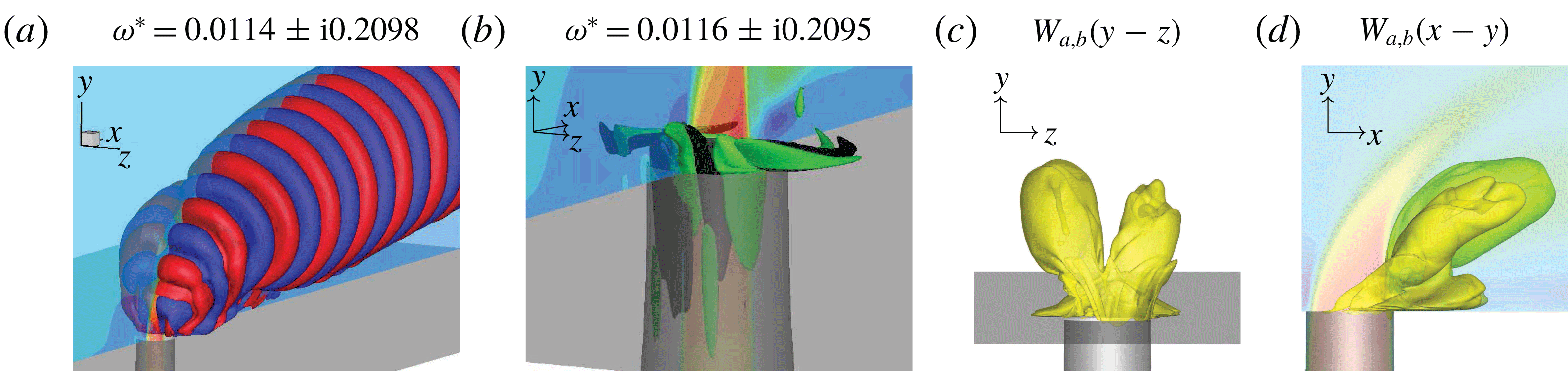
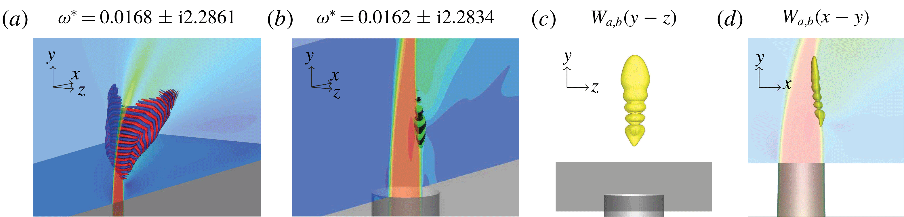
Figure 16 shows one of the pairs of downstream linear stability and adjoint sensitivity eigenmodes that have lower frequencies and longer length scales as compared to those previously discussed for case
 $R2$
. Additionally, they persist far downstream along the wall. Adjoint sensitivity analysis (figure 16
b) reveals sensitivities in the jet nozzle near the exit, but also in the region where the incoming cross-flow wraps around the jet nozzle exit, hinting at an increased sensitivity to perturbations from within the cross-flow boundary layer. The wavemaker region (figure 16
c,d) reveals some minor asymmetries in the sensitivity to localized feedback, but is largely symmetric between each side of the CVP.
Similar to figure 7, but for a representative pair of
 $R2$
downstream eigenmodes.

Similar to figure 7, but for the
 $R4$
lowest frequency eigenmodes.

Looking at case
 $R4$
, the lowest frequency pair of eigenmodes is shown in figure 17. The linear stability analysis eigenmode (figure 17
a) has larger spatial length scales than all previous eigenmodes, and also branches downwards towards the wall. There is a bias towards the right-hand side of the symmetry plane. However, this likely only implies that there is another set of eigenmodes that are biased towards the left-hand side of the symmetry plane, but with a growth rate smaller than that of the resolved eigenvalues. Adjoint sensitivity analysis (figure 17
b) shows that the largest sensitivity is not around the jet nozzle exit, but is upstream of the jet nozzle exit within the cross-flow boundary layer. Fric & Roshko (Reference Fric and Roshko1994) performed experiments that studied the wake vortices of the JICF by seeding the incoming cross-flow boundary layer and discovered that wake vortices could be visualized, leading to the conclusion that fluid inside the incoming cross-flow boundary layer travelled downstream to form wake vortices. Adjoint sensitivity analysis results add to these experimental results by showing there is a connection between perturbations in the cross-flow boundary layer and downstream of the jet exit near the wall. The wavemaker highlights the asymmetry, which implies that it is likely that a mirrored low-frequency pair of eigenmodes also exists.
4.4 Downstream shear layer
First shown by Regan & Mahesh (Reference Regan and Mahesh2017), the eigenvalue with the highest growth rate for case
 $R4$
is associated with the downstream shear layer and is shown in figure 18(a). As
 $R$
approaches infinity, the JICF becomes a free jet, and the upstream and downstream sides become indistinguishable. The magnitude of shear in the downstream shear layer is typically higher for case
 $R4$
compared to case
 $R2$
(see figure 45
d in appendix C). This makes the downstream shear layer dynamically more important for case
 $R4$
compared to case
 $R2$
. The linear stability mode is elevated from the jet nozzle exit and is located along the downstream side of the jet. This instability is most sensitive at the formation of the downstream shear layer. This region would be difficult to actuate in a control application, since it would most likely be invasive to the flow field.


The wavemaker is located where the downstream shear layer forms. By building upon the previous analysis, figure 18(c,d) shows the localization of the wavemaker, which has a strong resemblance to the absolutely unstable upstream shear layer of case
 $R2$
(figure 7). This is yet another reason to identify this region of the downstream shear layer as absolutely unstable. Furthermore, an extension to higher values of
 $R$
would suggest that a critical value
 $R_{crit}$
exists, at which point the downstream shear-layer region becomes convectively unstable.
5 Optimal perturbation analysis of the JICF
The JICF is studied using optimal perturbation analysis in this section. Several different optimization times are chosen relative to the characteristic time scale of the upstream shear-layer roll-up. In this section, the results are introduced and the observed growth is verified. Optimal perturbations for cases
 $R2$
and
 $R4$
are then discussed separately in §§ 5.1 and 5.2.
Global optimal perturbation analysis is performed for the same cases described in table 1. The same turbulent mean flows from adjoint sensitivity analysis are used as the base flows for optimal perturbation analysis, using the 138-million-element grid.
For cases
 $R2$
and
 $R4$
, the
 $19$
leading perturbations were computed to a maximum residual of
 $10^{-14}$
. Forty Arnoldi vectors were generated for each iteration in the IRAM. The time step sizes for each value of
 $R$
from the direct and adjoint analyses used were for the optimal perturbation analyses. For optimal perturbation analysis the LNS equations (2.2) were integrated
 $\unicode[STIX]{x1D70F}$
time units (non-dimensionalized by
 $D/v_{jet,max}$
) and then the adjoint LNS equations (2.7) were used to integrate backwards
 $\unicode[STIX]{x1D70F}$
time units for each Arnoldi vector. Different
 $\unicode[STIX]{x1D70F}$
values were chosen relative to the observed frequency of the upstream shear layer. The Strouhal numbers present in the upstream and downstream shear layers give guidance to the temporal scales of the JICF. Probing in the regions of the upstream and downstream shear layers gives
 $St_{up}$
and
 $St_{dn}$
, respectively. For case
 $R2$
,
 $1/St_{up}=1.54$
, and for case
 $R4$
,
 $1/St_{up}=1.28$
and
 $1/St_{dn}=0.44$
. This allowed study of optimal perturbations over times less than, equal to and greater than the characteristic time scale for each case.
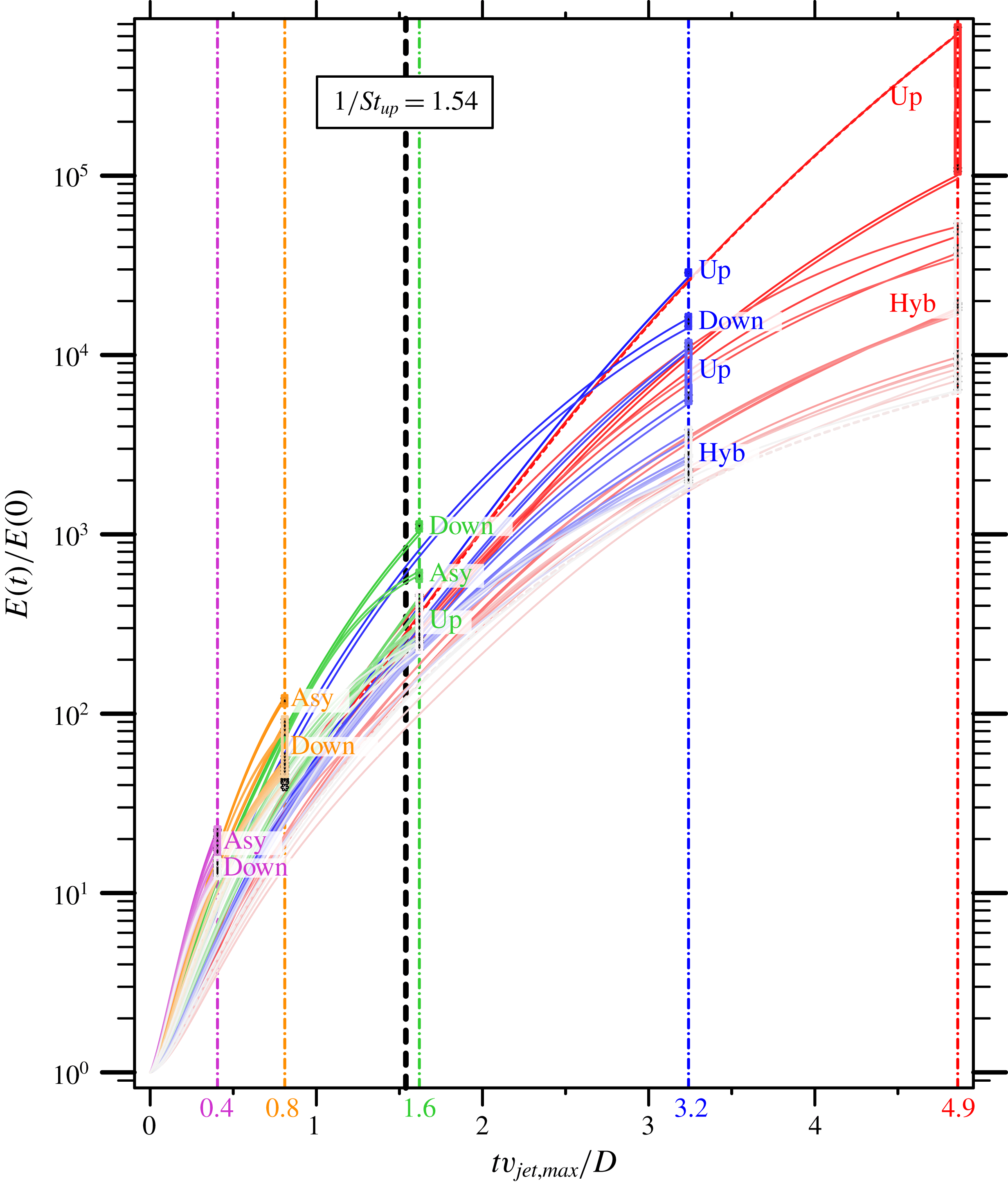
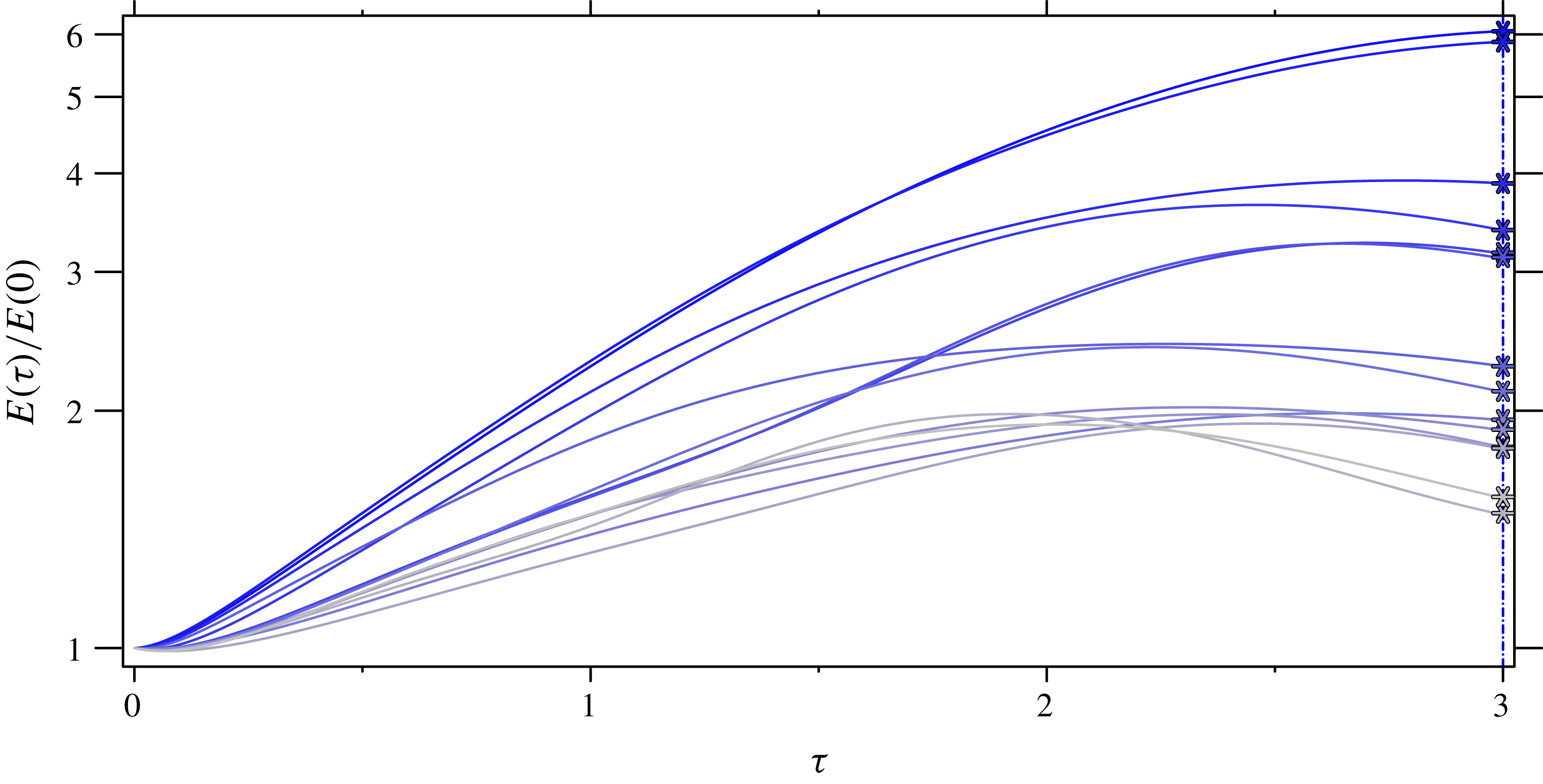
Transient growth is shown for case
 $R2$
, optimized for different
 $\unicode[STIX]{x1D70F}$
, which are differentiated by colour and the vertical dash-dotted lines. Additionally, the upstream shear-layer characteristic time scale,
 $1/St_{up}$
, is shown as a vertical black dashed line to provide temporal context. Eigenvalues for different
 $\unicode[STIX]{x1D70F}$
are shown on their associated vertical lines. Note that ‘Up’ and ‘Down’ refer to perturbations that act in the upstream and downstream shear layers, respectively. Also, ‘Hyb’ and ‘Asy’ refer to hybrid modes that act on both shear-layer and asymmetric perturbations, respectively.

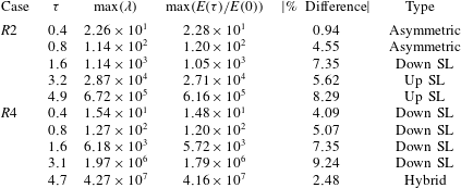
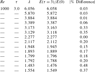
Details are shown for optimal perturbation analysis used to study the transient stability of the JICF. Several different time horizons are chosen that are shorter and longer than the characteristic time scale of the upstream shear layer,
 $1/St_{up}$
(see text). Additionally, the leading eigenvalue
 $\unicode[STIX]{x1D706}$
and the observed energy growth are compared as a % difference of
 $\unicode[STIX]{x1D706}$
. Note that the upstream shear layer and downstream shear layer are abbreviated as ‘Up SL’ and ‘Down SL’, respectively.

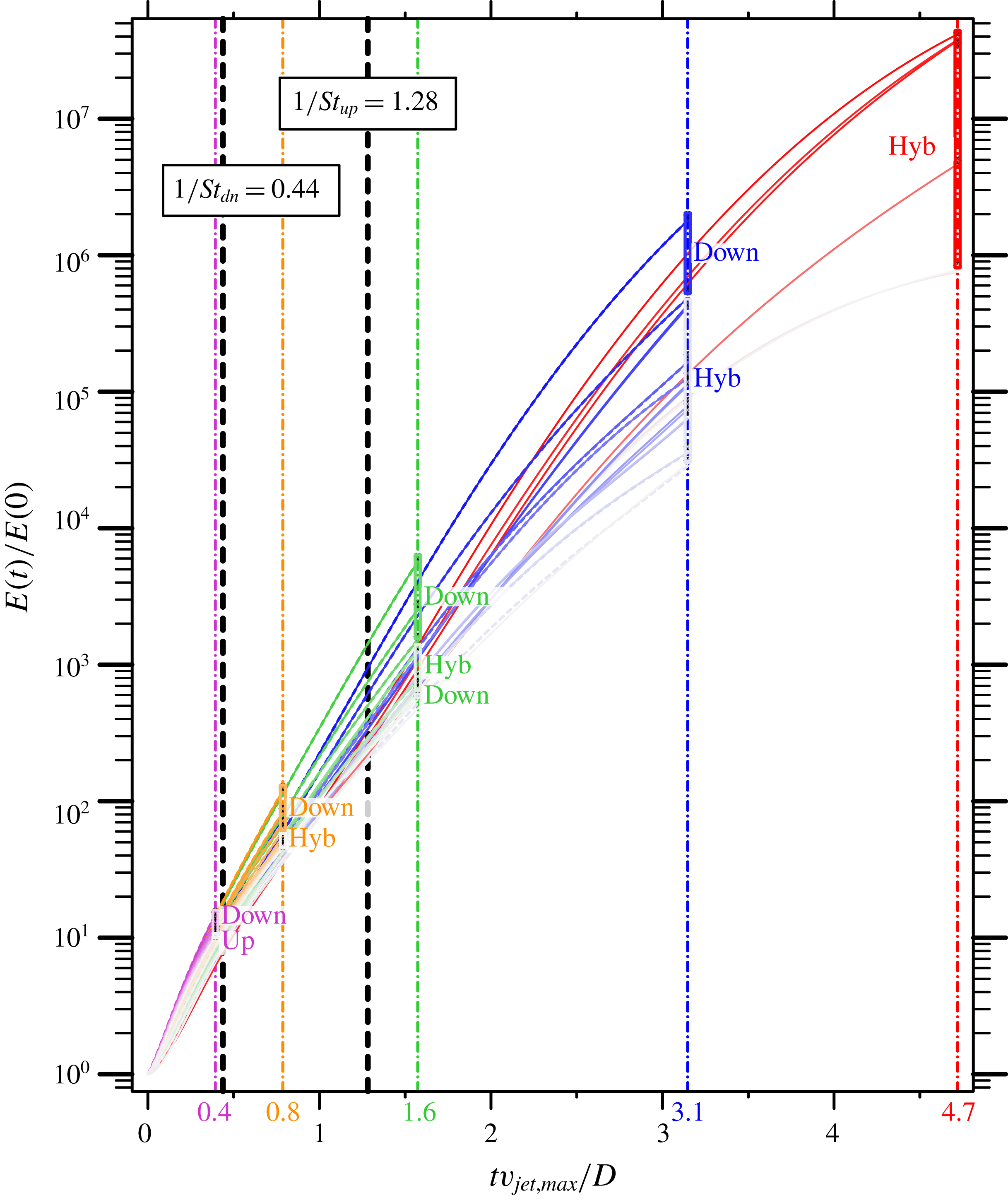
Figures 19 and 20 show the results from optimal perturbation analysis for the different
 $\unicode[STIX]{x1D70F}$
outlined in table 2. Note that the horizontal axis is linear in time, and the vertical axis is logarithmic in energy growth. Different colours are used for different values of
 $\unicode[STIX]{x1D70F}$
, with vertical dash-dotted lines in the same colour intercepting the
 $x$
-axis at
 $\unicode[STIX]{x1D70F}$
. Along the vertical coloured lines, the eigenvalues are plotted in order to make a visual comparison between the eigenvalue
 $\unicode[STIX]{x1D706}$
from optimal perturbation analysis and the energy growth obtained by applying the associated perturbation to the base flow, and integrating over the time
 $\unicode[STIX]{x1D70F}$
using the LNS equations. Additionally, each eigenvalue is labelled with a short description of the optimal perturbation shape, with similar modes grouped together. Finally, the characteristic time scale of the upstream shear layer is marked with a vertical dashed line in black.
Similar to figure 19, but for case
 $R4$
. Additionally, the time scale of the downstream shear layer,
 $1/St_{dn}$
, is shown as another vertical black dashed line.

Table 2 also describes the maximum growth observed for different
 $\unicode[STIX]{x1D70F}$
, and how well the eigenvalue and observed growth agree. Overall, good agreement is observed as the error is shown to be less than
 $10\,\%$
. For a computational domain with inflow and outflow boundaries, this error is reasonable due to the fact that any perturbation that escapes the domain will no longer be included in the overall perturbation kinetic energy. To reduce the amount of error between the eigenvalue and observed growth, the domain would need to be extended to allow perturbations to travel further before escaping the computational domain. This effect can be observed in table 2 by noting how the % difference is generally larger for greater values of
 $\unicode[STIX]{x1D70F}$
.
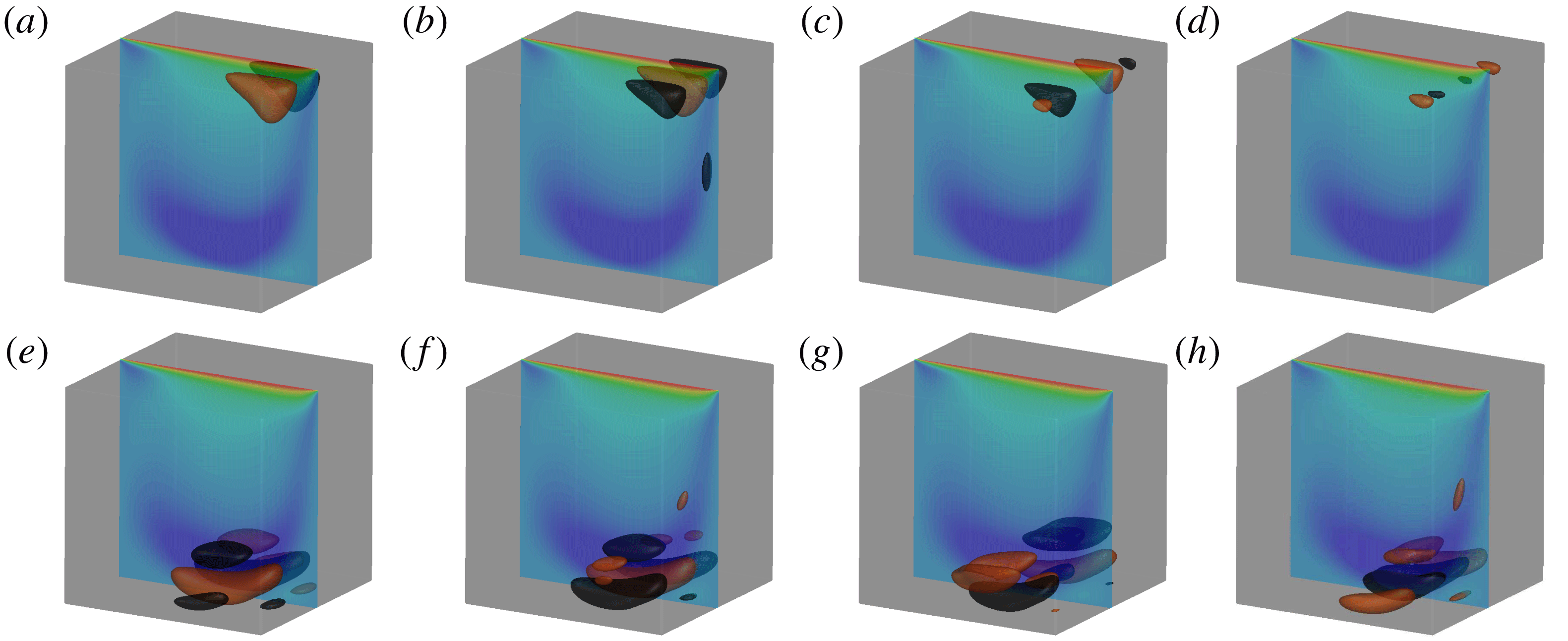
In the following subsections, these figures and the associated optimal perturbation modes are discussed in detail. Both cases are organized into three subsections describing short, characteristic and long time horizons. The optimal perturbation modes are shown using either an isometric view or a side-view in an
 $xy$
-plane. Also, they are visualized using isocontours of the vertical perturbation velocity,
 $\tilde{v}$
, at levels equal to
 $\pm 0.001$
coloured as orange and black, respectively. Additionally, for the isometric view, contours of the vertical velocity of the base flow,
 $\overline{v}$
, are shown for the symmetry plane at
 $z=0$
.
5.1 Optimal perturbations for case
 $R2$

Figure 19 suggests some overall conclusions from optimal perturbation analysis of case
 $R2$
. For short times (i.e.
 $\unicode[STIX]{x1D70F}<1/St_{up}$
), asymmetric perturbations dominate where the CVP forms, with sub-optimal perturbations growing along the downstream shear layer. For
 $\unicode[STIX]{x1D70F}=0.8$
, there are sub-optimal modes that symmetrically perturb both the downstream shear layer and the CVP. Not until the characteristic time scale (i.e.
 $\unicode[STIX]{x1D70F}\approx 1/St_{up}$
) does perturbing the downstream shear layer become optimal. On this time scale, it becomes clear from figure 19 that asymmetric perturbations of the CVP are sub-optimal. This gives rise to other sub-optimal perturbations of the upstream shear layer that quickly become significant for larger time scales. When optimal perturbations are considered for long time horizons (i.e.
 $\unicode[STIX]{x1D70F}>1/St_{up}$
), the modes result in growth along the upstream shear layer. Furthermore, sub-optimal perturbations move from the downstream shear layer to complex perturbations with higher circumferential wavenumbers along the upstream shear layer for
 $3.2\leqslant \unicode[STIX]{x1D70F}\leqslant 4.9$
. Finally, the group of perturbations that have the lowest growth factors include a series of hybrid perturbations that grow along both the upstream and downstream shear layers, as well as a series of increasing circumferential wavenumbers. The three time horizons are discussed in detail below.
5.1.1 Short time horizon
For the short time horizon, optimal perturbations take advantage of mechanisms that act much faster than the characteristic time scale
 $1/St_{up}=1.54$
to produce energy. First and foremost are the asymmetric perturbations, which dominate energy growth over the short time scales
 $0.4\leqslant \unicode[STIX]{x1D70F}\leqslant 0.8$
. The states of these perturbations at
 $\unicode[STIX]{x1D70F}=0.8$
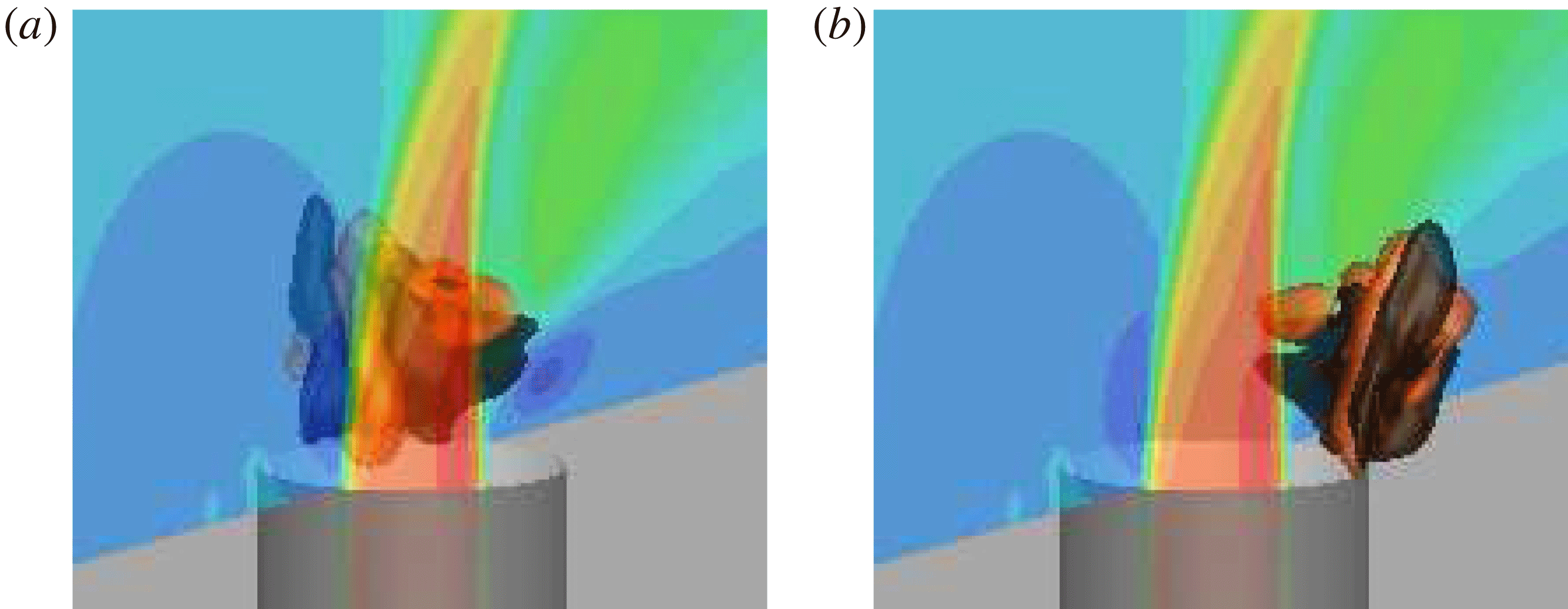
are shown in figure 21. These perturbations ride along the CVP in the base flow as they propagate in helical fashion downstream. Not only are there pairs of asymmetric perturbations, but a series of increasing circumferential wavenumbers characterize the next few sub-optimal eigenmodes for
 $\unicode[STIX]{x1D70F}=0.4$
(not shown). The asymmetric perturbations originate at the jet nozzle exit and propagate downstream on either side of the CVP.
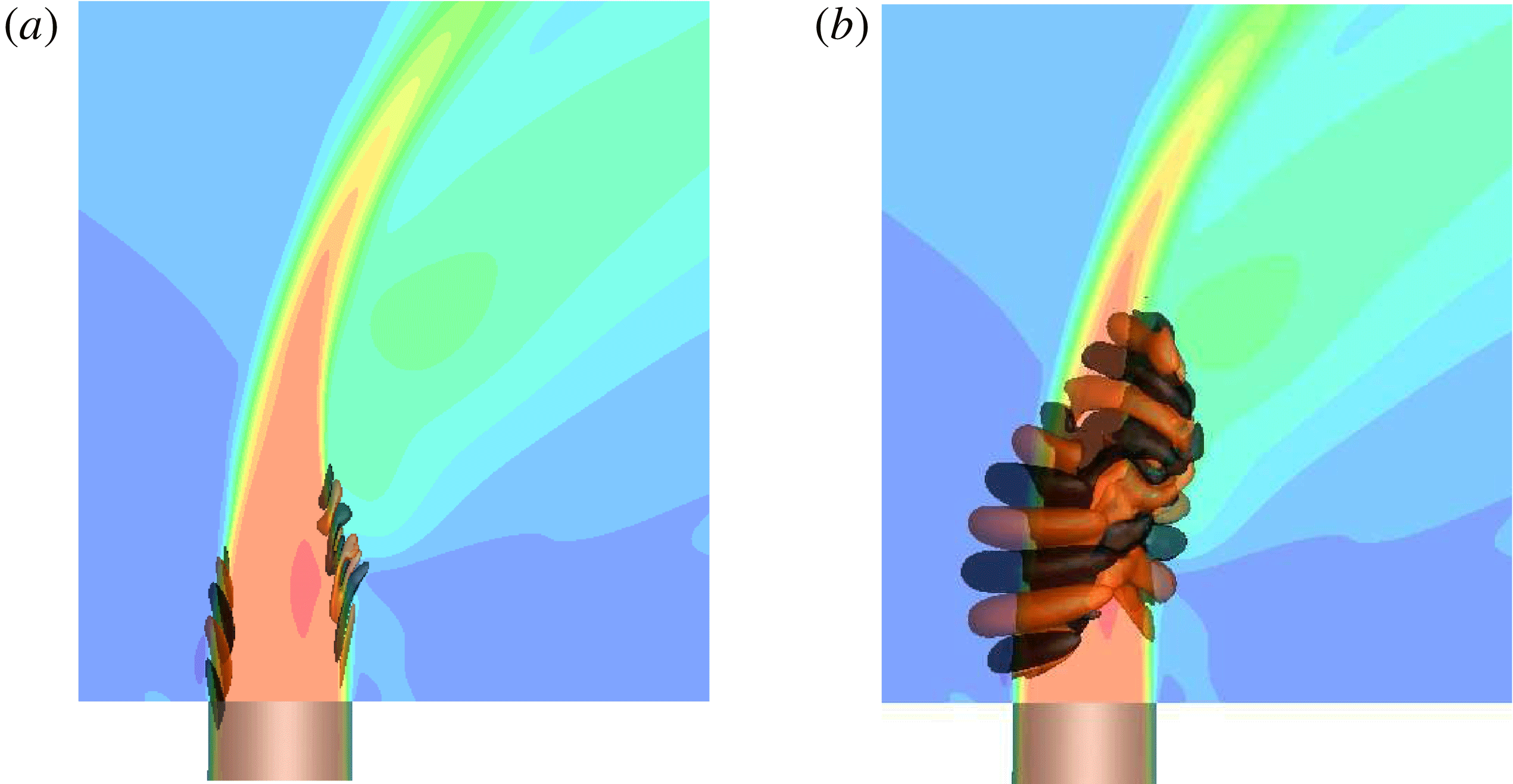
Case
 $R2$
, short time horizon,
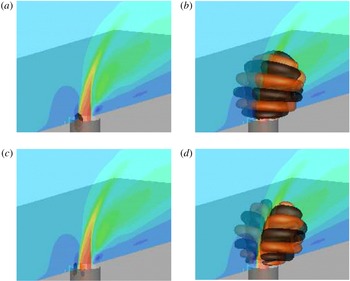
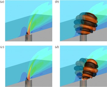
 $\unicode[STIX]{x1D70F}=0.8$
, final state of the first (a) and the second (b) leading asymmetric perturbations.

The next sub-optimal perturbations for
 $\unicode[STIX]{x1D70F}=0.8$
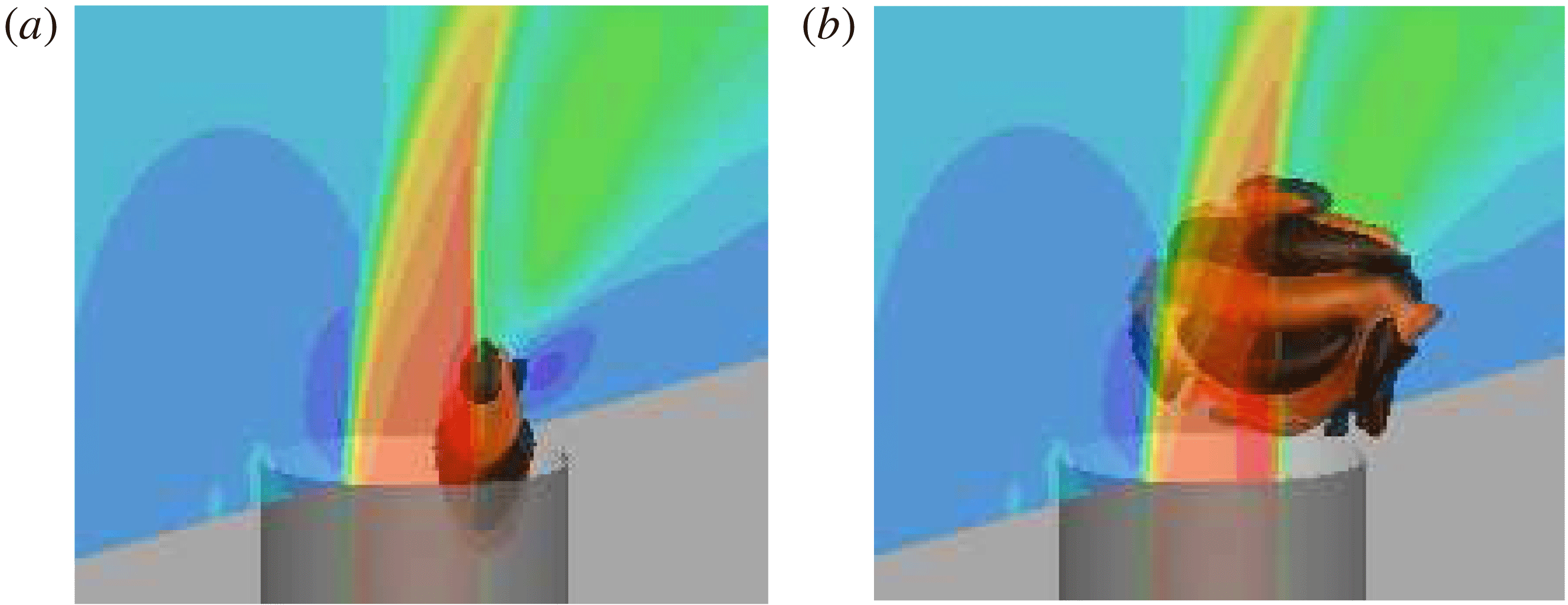
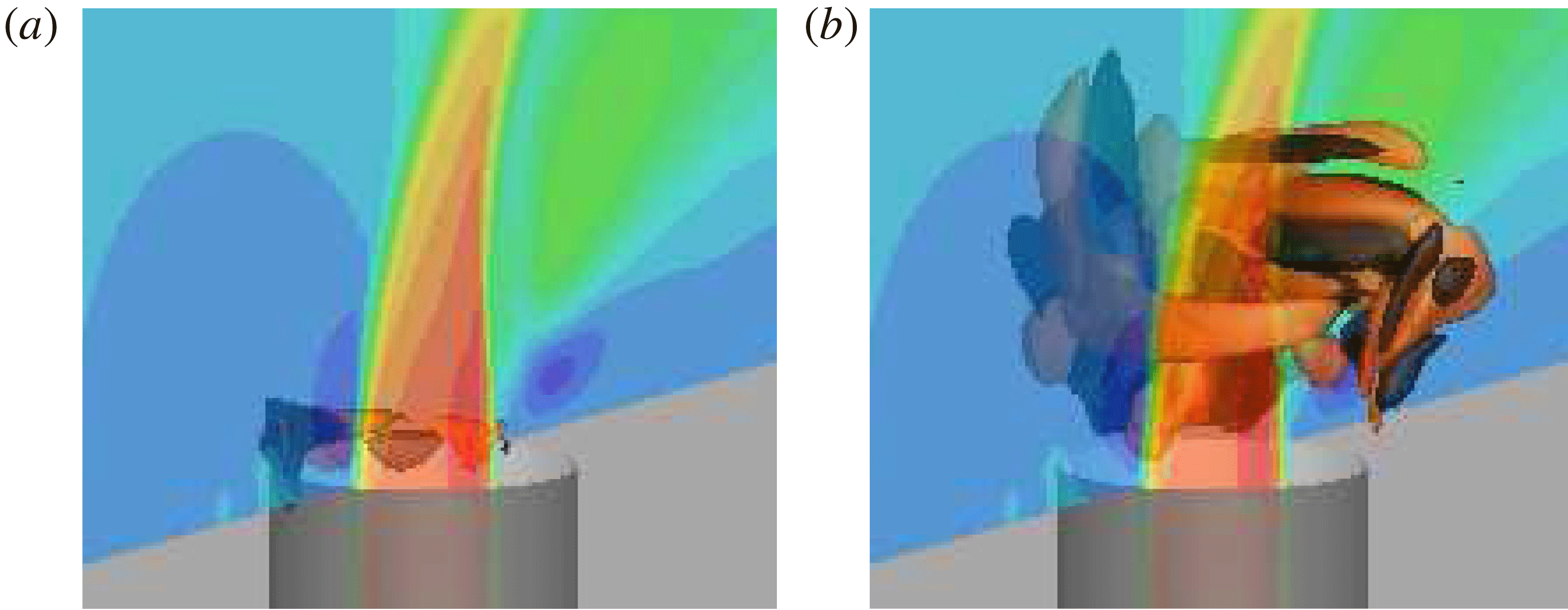
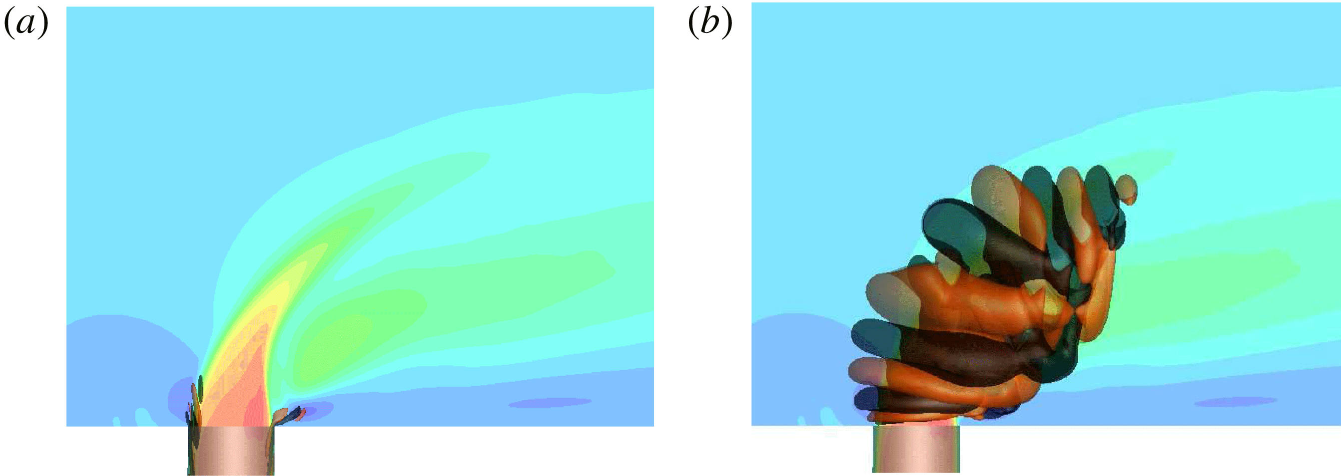
grow along the downstream shear layer, which are shown in figure 22. The evolution of the downstream shear layer perturbations is characteristic of the downstream shear-layer roll-up observed in DNS (figure 4
a). These perturbations originate within the nozzle on the downstream side as shown in figure 22. For
 $\unicode[STIX]{x1D70F}=0.4$
, the sub-optimal downstream shear-layer perturbation generates
 ${\approx}68\,\%$
of the energy growth compared to the asymmetric perturbation. Comparatively, when
 $\unicode[STIX]{x1D70F}=0.8$
, the sub-optimal downstream shear-layer perturbation (figure 22) generates
 ${\approx}73\,\%$
of the energy growth compared to the optimal asymmetric perturbation (figure 21). This highlights the fact that as
 $\unicode[STIX]{x1D70F}$
increases the downstream perturbations are becoming efficient at producing energy.
Case
 $R2$
, short time horizon,
 $\unicode[STIX]{x1D70F}=0.8$
, origination (a) and final state (b) of the sub-optimal downstream shear-layer perturbation.

The least effective sub-optimal perturbations that generate the lowest energy growth for
 $0.4\leqslant \unicode[STIX]{x1D70F}\leqslant 0.8$
include a series of hybrid and higher wavenumber versions of the previously shown perturbations. For
 $\unicode[STIX]{x1D70F}=0.4$
, the least efficient perturbations are the hybrid perturbations that generate energy from both the CVP and the downstream shear layer. The results are similar for
 $\unicode[STIX]{x1D70F}=0.8$
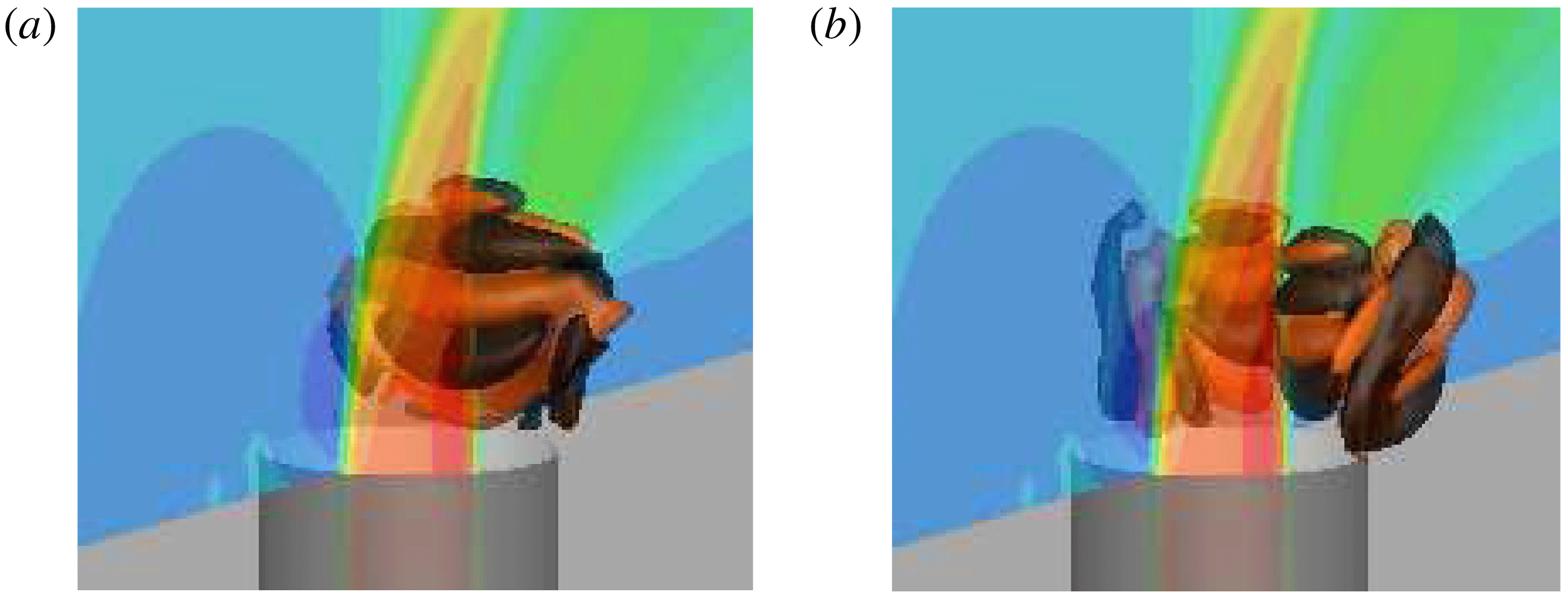
, which have a series of hybrid CVP and downstream shear-layer perturbations shown in figure 23 with increasing wavenumbers and decreasing growth factors.
Case
 $R2$
, short time horizon,
 $\unicode[STIX]{x1D70F}=0.8$
, final state of the first (a) and the second (b) sub-optimal asymmetric perturbations.

5.1.2 Characteristic time horizon
The characteristic-time-scale optimal perturbations take advantage of processes that act on times of the order of the characteristic time scale
 $1/St_{up}=1.54$
to increase energy. As
 $\unicode[STIX]{x1D70F}$
is increased beyond the short time scale, there is a bifurcation. The highest energy growth optimal modes change from asymmetric perturbations (figure 25) to perturbations that grow along the downstream shear layer (figure 24). Figure 19 clearly shows the significant drop in energy growth for the asymmetric perturbations, which are now sub-optimal for
 $\unicode[STIX]{x1D70F}=1.6$
.
Case
 $R2$
, characteristic time horizon,
 $\unicode[STIX]{x1D70F}=1.6$
, origination (a) and final state (b) of the optimal downstream shear-layer perturbation.

Case
 $R2$
, characteristic time horizon,
 $\unicode[STIX]{x1D70F}=1.6$
, initial (a) and final (b) state of a sub-optimal hybrid asymmetric downstream shear-layer perturbation. Note that there is a second perturbation that is mirrored across the
 $z=0$
plane.

Sub-optimal perturbations of the upstream shear layer are found for the first time in the optimal analysis at the characteristic time scale. The upstream shear-layer sub-optimal modes are shown in figure 26, arranged with decreasing energy growth and increasing circumferential wavenumbers. It is significant that higher wavenumber counterparts to the upstream shear-layer mode are also found. This shows that the upstream shear-layer region is becoming a significant energy growth opportunity since higher wavenumber downstream shear-layer and asymmetric perturbations are no longer recovered in the analysis.
Case
 $R2$
, characteristic time horizon,
 $\unicode[STIX]{x1D70F}=1.6$
, initial (a) and final (b) state of the sub-optimal upstream shear-layer perturbation, along with the initial (c) and final (d) state of a higher circumferential wavenumber counterpart with a smaller growth factor.

5.1.3 Long time horizon
The long-time-scale optimal perturbations take advantage of processes that act on larger times than the characteristic time scale
 $1/St_{up}=1.54$
. Another bifurcation in optimal perturbation analysis for case
 $R2$
happens over the long time horizon. In the range
 $1.6\leqslant \unicode[STIX]{x1D70F}\leqslant 3.2$
the optimal perturbations change from acting along the downstream shear layer (figure 27) to the upstream shear layer (figure 28). Also, there are several higher wavenumber counterparts to the upstream shear-layer optimal perturbations (not shown).
Case
 $R2$
, long time horizon,
 $\unicode[STIX]{x1D70F}=3.2$
, origination (a) and final state (b) of the sub-optimal downstream shear-layer optimal perturbation.

Case
 $R2$
, long time horizon,
 $\unicode[STIX]{x1D70F}=3.2$
, the initial (a) and final (b) state of the upstream shear-layer optimal perturbation, along with the initial (c) and final (d) state of a lower growth factor perturbation with a higher circumferential wavenumber.

The least effective perturbations generate energy along the upstream and downstream shear layers simultaneously. For the longest time horizon that was studied for case
 $R2$
, the optimal perturbations again act along the upstream shear layer to generate the most energy growth, which are visualized in figure 29. This is consistent with the results from the linear stability and adjoint sensitivity analyses in § 4, which examined the stability and sensitivity at the asymptotic limit of time. Note that the first few sub-optimal perturbations are also upstream shear-layer modes with higher circumferential wavenumbers, one of which is shown in figures 29(c) and 29(d) for its initial and final states, respectively.
Case
 $R2$
, long time horizon,
 $\unicode[STIX]{x1D70F}=4.9$
, initial (a) and final (b) state of the upstream shear-layer optimal perturbation, along the initial (c) and final (d) state of a lower growth factor perturbation with a higher circumferential wavenumber.

Figure 30 shows one of the remaining sub-optimal perturbations that are a set of hybrid upstream and downstream shear-layer modes. For these modes, there are no longer any purely downstream shear-layer perturbations. Instead, perturbations act on both the upstream and downstream side of the jet nozzle exit (figure 30 a) to generate growth along the jet trajectory (figure 30 b).
Case
 $R2$
, long time horizon,
 $\unicode[STIX]{x1D70F}=4.9$
, origin (a) and final state (d) of the sub-optimal hybrid shear-layer perturbation.

5.2 Optimal perturbations for case
$R4$

Similar to case
 $R2$
, some overall conclusions from optimal perturbation analysis for case
 $R4$
are highlighted using figure 20. Short-time-horizon optimal perturbations are dominated by growth along the downstream shear layer for
 $0.4\leqslant \unicode[STIX]{x1D70F}\leqslant 0.8$
. However, there are sub-optimal perturbations that grow along the upstream shear layer, as well as hybrid perturbations for both shear layers when
 $\unicode[STIX]{x1D70F}=0.8$
. For the characteristic time scale, the downstream shear-layer growth again dominates. However, a group of sub-optimal hybrid perturbations also have significant growth. For
 $\unicode[STIX]{x1D70F}=1.6$
, there are no longer purely upstream shear-layer sub-optimal modes, only hybrids that grow along the upstream and downstream shear layers. Over the long time horizons, it is shown that all optimal perturbations are some form of hybrid mode. When
 $\unicode[STIX]{x1D70F}=3.1$
, there is often a bias towards either the upstream or downstream shear layers. However, for
 $\unicode[STIX]{x1D70F}=4.7$
, the hybrid modes have less significant biases, with a more evenly spread perturbation across the upstream and downstream shear layers.
5.2.1 Short time horizon
The short-time-scale optimal perturbations take advantage of processes that act on times shorter than the characteristic time scale (i.e. less than
 $1/St_{up}=1.28$
) to increase energy. Unlike case
 $R2$
, there are no asymmetric perturbation modes. Instead, the short-time-scale (
 $0.4\leqslant \unicode[STIX]{x1D70F}\leqslant 0.8$
) optimal modes, and the first few sub-optimal modes, generate energy growth as they propagate along the downstream shear layer. The group of downstream shear-layer modes for
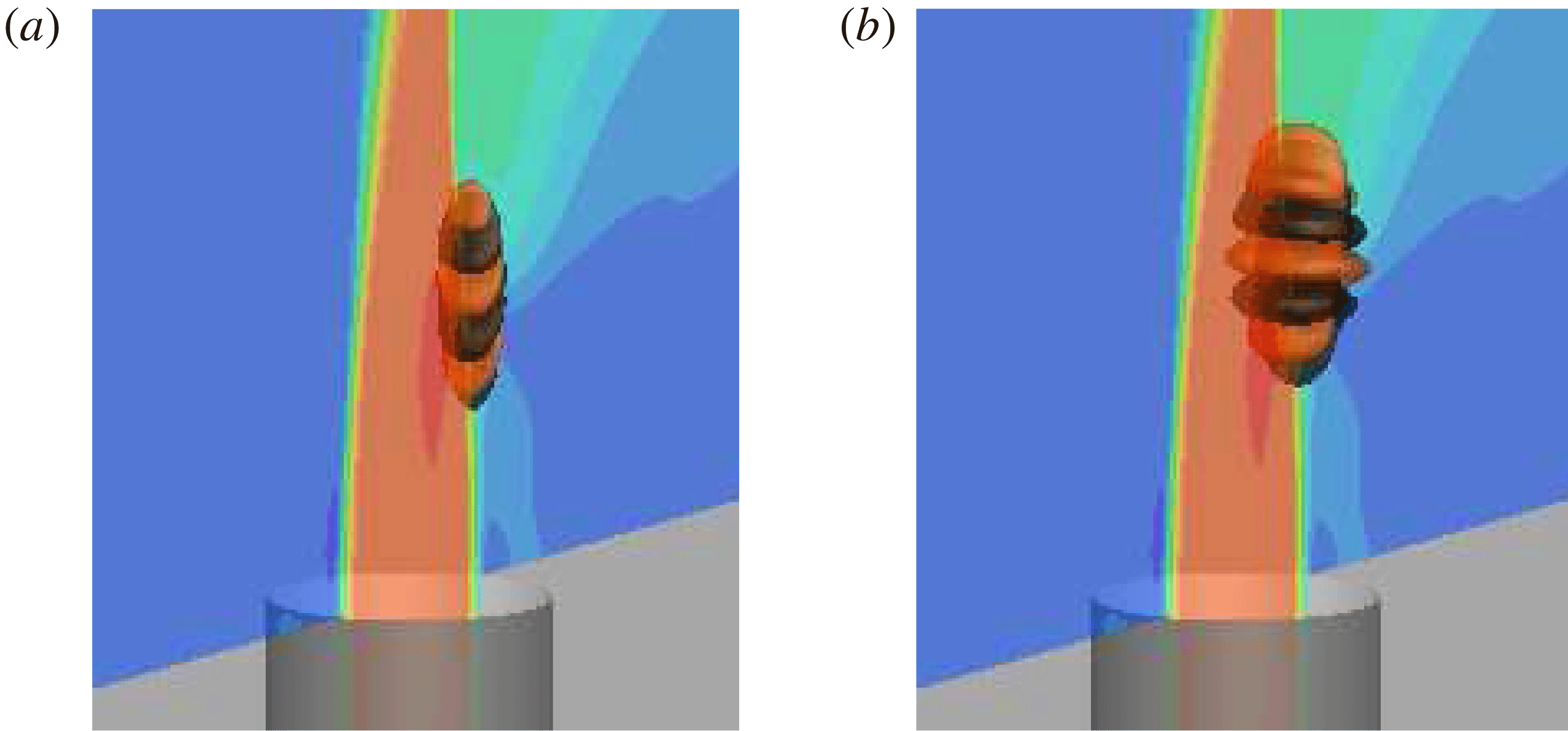
 $\unicode[STIX]{x1D70F}=0.4$
are shown in figure 31, and for
 $\unicode[STIX]{x1D70F}=0.8$
in figure 32. For this short time, the perturbation modes do not have much time to advect along the base flow, which results in the focus on the downstream shear layer to generate growth.
Case
 $R4$
, short time horizon,
 $\unicode[STIX]{x1D70F}=0.4$
, origination (a) and final state (b) of the leading downstream shear-layer perturbation.

Case
 $R4$
, short time horizon,
 $\unicode[STIX]{x1D70F}=0.8$
, origination (a) and final state (b) of the leading downstream shear-layer perturbation.

The next few sub-optimal perturbation modes make use of the upstream shear layer to grow on top of the base flow. For
 $\unicode[STIX]{x1D70F}=0.8$
, figure 33(a) shows a sub-optimal perturbation mode with no circumferential wavenumber that generates the highest growth compared to its higher wavenumber counterparts (figure 33
b).
Case
 $R4$
, short time horizon,
 $\unicode[STIX]{x1D70F}=0.8$
, initial (a) and final (b) state of sub-optimal upstream shear-layer perturbation, along with the initial (c) and final (d) state of a lower growth factor perturbation with a circumferential wavenumber.

5.2.2 Characteristic time horizon
Optimal perturbations on the characteristic time horizon take advantage of processes that act on times of the order of the characteristic time scale,
 $1/St_{up}=1.28$
, to increase energy. The optimal perturbations are again a group of modes that grow along the downstream shear layer. Figure 34 shows the leading optimal perturbation for
 $\unicode[STIX]{x1D70F}=1.6$
, along with the first few sub-optimal modes which also grow predominately along the downstream shear layer, but with higher circumferential wavenumbers.
Case
 $R4$
, characteristic time horizon,
 $\unicode[STIX]{x1D70F}=1.6$
, initial (a) and final (b) state of the downstream shear-layer optimal perturbation, as well as the initial (c) and final (d) state of a sub-optimal perturbation with a smaller growth factor and higher circumferential wavenumber.

The remaining sub-optimal perturbation modes are all hybrid perturbation modes that show growth along upstream and downstream shear layers simultaneously. The hybrid perturbation with the largest growth factors is presented in figure 35. Hybrid modes have varying biases towards the upstream and downstream shear layers, and thus have slightly different evolutions. Interestingly, the final states of the perturbations at time
 $\unicode[STIX]{x1D70F}$
are optimized so that the upstream and downstream perturbations propagate along the shear layers and meet up at the collapse of the potential core.
Case
 $R4$
, characteristic time horizon,
 $\unicode[STIX]{x1D70F}=1.6$
, origination (a) and final state (b) of a sub-optimal hybrid shear-layer perturbation.

5.2.3 Long time horizon
The long-time-scale optimal perturbations take advantage of processes that act on times longer than the characteristic time scale
 $1/St_{up}=1.28$
. The optimal perturbation for
 $\unicode[STIX]{x1D70F}=3.1$
continues to take advantage of the downstream shear layer as the only path to generate energy growth. The initial perturbation (figure 36) is elevated from the jet nozzle exit and grows significantly around the downstream shear layer as it travels further downstream. The sub-optimal hybrid perturbation with the largest growth factor is shown in figure 37; the other sub-optimal perturbations for
 $\unicode[STIX]{x1D70F}=3.1$
(not shown) again have different biases towards the upstream and downstream shear layers.
Case
 $R4$
, long time horizon,
 $\unicode[STIX]{x1D70F}=3.1$
, origination (a) and final state (b) of the downstream shear-layer optimal perturbation.

Case
 $R4$
, long time horizon,
 $\unicode[STIX]{x1D70F}=3.1$
, sub-optimal hybrid shear-layer perturbation with the largest growth factor.

For the longest time horizon of
 $\unicode[STIX]{x1D70F}=4.7$
for case
 $R4$
, all of the perturbations are shown to grow in energy along both upstream and downstream shear layers (figure 38). The initial perturbations of the hybrid modes (leading mode shown in figure 38
a) show biases towards both the shear layers, but their evolutions (leading mode shown in figure 38
b) are qualitatively similar. Therefore, for long time horizons for case
 $R4$
, the best way to perturb the base flow is to simultaneously perturb the upstream and downstream shear layers. This is consistent with the results from linear stability and adjoint sensitivity analyses in figure 6(b), which highlights that the upstream and downstream shear-layer instability modes have similar growth rates.
Case
 $R4$
, long time horizon,
 $\unicode[STIX]{x1D70F}=4.7$
, the initial perturbation (a) and the associated final state (b) are shown for sub-optimal hybrid shear-layer perturbation with the largest growth factor.

6 Summary
Understanding the stability and sensitivity of JICF is critical for developing control strategies to optimize performance in engineering applications. Low-speed JICF is studied from a global perspective using linear stability, adjoint sensitivity and optimal perturbation analyses. The global modes from linear stability analysis highlight the regions where the largest growth is observed asymptotically. This provides insight into the best placement of sensors for measuring the flow state. The frequencies of upstream shear-layer linear stability analysis eigenmodes agree well with past DNS (Iyer & Mahesh Reference Iyer and Mahesh2016) and experiments (Megerian et al.
Reference Megerian, Davitian, Alves and Karagozian2007). The linear stability analysis results show that case
 $R2$
is dominated by the upstream shear-layer instability. However, there are other eigenmodes that are asymmetric across the mid-plane and much lower frequency modes that travel far downstream and have finger-like fluid structures resembling wake vortices. In addition to an upstream shear-layer instability mode, case
 $R4$
also has a downstream shear-layer instability with a higher growth rate. Furthermore, the asymmetric instabilities for case
 $R4$
have higher relative growth rates than that of case
 $R2$
, highlighting their increased significance to the overall dynamics. This behaviour also suggests an explanation for the asymmetric CVP eigenmodes that were previously observed in experiments at higher
 $R$
.
Adjoint sensitivity analysis results are complementary, as they provide sensitivity information that outlines the regions where the linear stability analysis modes are sensitive to momentum forcing. This information is valuable for efficient actuator placement. The upstream shear-layer modes for both cases are most sensitive along the upstream side of the jet nozzle exit. The asymmetric modes for both cases are most sensitive on each side of the upstream side of the jet nozzle exit. For case
 $R4$
, the downstream shear layer is most receptive to actuation at an elevated position from the jet nozzle exit on the downstream side. Interestingly, the low-frequency modes are sensitive to perturbations on the upstream side of the jet nozzle, and wrap around to the outer edge. For case
 $R4$
, the low-frequency modes are sensitive to an extended region upstream of the jet nozzle exit in the incoming cross-flow, highlighting the connection to perturbations in the cross-flow on the fluid structures that resemble wake vortices.
The linear stability and adjoint sensitivity analyses can be used in tandem to compute wavemaker regions. The wavemaker regions for the upstream shear-layer modes are qualitatively different for cases
 $R2$
and
 $R4$
. For case
 $R2$
, the wavemaker region is concentrated to a small region near the upstream edge of the jet nozzle exit where the upstream shear layer is formed. Conversely, case
 $R4$
has a wavemaker region that extends along a considerable length of the upstream shear layer. These differences are consistent with the stability transition of the upstream shear layer. Additionally, the wavemaker regions provide insight into the regions that are most receptive to retaining and amplifying frequencies that are induced upon them.
Optimal perturbation analysis examines the stability and sensitivity at finite time scales to determine the ‘most dangerous’ disturbances for the JICF. The optimal perturbations provide additional information about the regions that are most sensitive to actuation. The evolutions of the perturbations highlight the paths that the perturbations follow to generate energy growth, and provide insight into actuation (initial state) and sensor placement (final state). For case
 $R2$
, the optimal perturbations for short time display the ability to grow along each half of the CVP by perturbing the left- and right-hand sides just above the downstream side of the jet nozzle exit. For time horizons of the order of the upstream shear-layer shedding period, the optimal actuation occurs along the downstream side of the jet nozzle exit, and results in growth along the downstream shear layer. For the longer time scales, hybrid perturbations that grow along the upstream and downstream shear layers simultaneously are the most optimal. For case
 $R4$
, the optimal perturbations along the downstream shear layer dominate for shorter time scales. However, for time scales longer than the characteristic time horizon, hybrid perturbations are again the most efficient at generating energy by leveraging growth along both shear layers.
Overall, the present work uses high-fidelity numerical methods and high-performance computing to study the stability and sensitivity of the low-speed JICF from a global perspective. The present results demonstrate state-of-the-art capabilities, and are the largest stability and sensitivity simulations performed to the best of our knowledge. Valuable insight gained from the stability and sensitivity analyses of the JICF can be used to optimize the placement of both sensors and actuators to efficiently manipulate the JICF.
Acknowledgements
This work was supported by AFOSR grant FA9550-15-1-0261. Simulation time was provided by the Texas Advanced Computing Center (TACC) through the Extreme Science and Engineering Discovery Environment (XSEDE) allocation. We thank Dr P. Kumar and S. Harel for their help during the revision of the manuscript.
Appendix A. Validation of adjoint sensitivity analysis
A.1 Blasius boundary layer
Hill (Reference Hill1995) studied the stability and sensitivity of the Blasius boundary layer. The parallel flow assumption is valid here, which allows us to assume streamwise homogeneity in the form of the wavenumber
 $\unicode[STIX]{x1D6FC}$
(no spanwise component). To be consistent with the study by Hill (Reference Hill1995), the following ansatz is defined for this validation case:
 $$\begin{eqnarray}\displaystyle \tilde{\boldsymbol{u}}_{i}^{\dagger }(x,y,t)=\mathop{\sum }_{\unicode[STIX]{x1D6FC},\unicode[STIX]{x1D714}}\hat{\boldsymbol{u}}_{i}^{\dagger }(y)\text{e}^{\text{i}\unicode[STIX]{x1D6FC}x+\unicode[STIX]{x1D714}t}+\text{c.c}. & & \displaystyle\end{eqnarray}$$
The base state is the Blasius boundary layer solution. Distances are non-dimensionalized by
 $\unicode[STIX]{x1D6FF}=\sqrt{\unicode[STIX]{x1D708}L/U_{\infty }}$
, where
 $L$
is the dimensional distance from the leading edge of the plate. The distance from the wall where
 $u=0.99U_{\infty }$
is
 $\unicode[STIX]{x1D6FF}_{99}=4.93\unicode[STIX]{x1D6FF}$
.
The Blasius boundary layer at
 $Re=U_{\infty }\unicode[STIX]{x1D6FF}/\unicode[STIX]{x1D708}=1274$
is subjected to a streamwise T-S wave with
 $f=\text{Im}(\unicode[STIX]{x1D714})/Re=20\times 10^{-6}$
. Here, an imaginary
 $\unicode[STIX]{x1D714}$
is prescribed, and
 $\unicode[STIX]{x1D6FC}$
is the complex eigenvalue, which makes this a spatial sensitivity problem. The leading adjoint eigenvalue calculated by Hill (Reference Hill1995) is
 $\unicode[STIX]{x1D6FC}=0.0895-\text{i}0.00377$
, compared to
 $\unicode[STIX]{x1D6FC}=0.0894-\text{i}0.00381$
from the present work. The associated adjoint eigenmodes (normalized by
 $\text{max}(|\hat{u} _{i}|)$
) show good agreement with Hill (Reference Hill1995) as shown in figure 39.
The eigenmodes obtained from spatial adjoint sensitivity analysis of a Blasius boundary at
 $Re=U_{\infty }\unicode[STIX]{x1D6FF}/\unicode[STIX]{x1D708}=1274$
subject to a T-S wave with
 $f=\text{Im}(\unicode[STIX]{x1D714})/Re=20\times 10^{-6}$
are compared to the results of Hill (Reference Hill1995) showing good agreement.

A.2 Laminar channel flow
The final validation problem compares two leading eigenvalues from direct parallel linear stability (Juniper, Hanifi & Theofilis Reference Juniper, Hanifi and Theofilis2014), global linear stability and the global adjoint sensitivity of laminar channel flow. The parallel flow assumption holds, and therefore the streamwise and spanwise directions can be assumed homogeneous. In other words, for the parallel flow analysis the following ansatz will be used:
 $$\begin{eqnarray}\displaystyle \tilde{\boldsymbol{u}}_{i}^{\dagger }(x,y,z,t)=\mathop{\sum }_{\unicode[STIX]{x1D6FC},\unicode[STIX]{x1D6FD},\unicode[STIX]{x1D714}}\hat{\boldsymbol{u}}_{i}^{\dagger }(y)\text{e}^{\text{i}(\unicode[STIX]{x1D6FC}x+\unicode[STIX]{x1D6FD}z)+\unicode[STIX]{x1D714}t}+\text{c.c}. & & \displaystyle\end{eqnarray}$$
However, in global linear stability and global adjoint sensitivity analyses, the ansatzes defined in § 2 ((2.3) and (2.8), respectively) are used.
A steady base flow is used in the stability and sensitivity analyses corresponding to the laminar channel flow at
 $Re=1000$
, based on the centreline velocity and the channel half-height (
 $h$
). The domain size is
 $4\unicode[STIX]{x03C0}h\times 2h\times 4h\unicode[STIX]{x03C0}/3$
in the streamwise, the wall-normal and the spanwise directions. Periodic boundary conditions are applied in the streamwise and the spanwise directions, and no-slip condition is applied at the walls.
Any combination of streamwise and spanwise wavenumbers may be present in the global linear stability and adjoint sensitivity results. However, the eigenmodes from global linear stability (figure 40
a) and global adjoint sensitivity (figure 41
a,b) are specifically chosen because they show clear streamwise (
 $\unicode[STIX]{x1D6FC}$
) and spanwise (
 $\unicode[STIX]{x1D6FD}$
) wavenumbers. These wavenumbers are recovered by performing a two-dimensional fast Fourier transform in the
 $x$
and
 $z$
directions. Next, the recovered
 $\unicode[STIX]{x1D6FC}$
and
 $\unicode[STIX]{x1D6FD}$
are used as input for the parallel flow linear stability analysis. A detailed description of the input parameters and eigenvalue results are shown in table 3.
Real part of the first adjoint eigenmode corresponding to the first adjoint sensitivity eigenvalue
 $\unicode[STIX]{x1D714}_{1}$
in table 3 for laminar channel flow at
 $Re=1000$
. The results are shown in
 $z=0$
plane with contours of
 $\tilde{w}^{\dagger }$
(note
 $\tilde{u} ^{\dagger }=\tilde{v}^{\dagger }=0$
). The streamwise and spanwise wavenumbers (
 $\unicode[STIX]{x1D6FC}=1$
,
 $\unicode[STIX]{x1D6FD}=0$
) are extracted and used as input to classic parallel flow stability analysis. The adjoint sensitivity eigenmode Fourier coefficients (
 $\hat{u} _{i}^{\dagger }$
) are also shown (b).

Two leading eigenvalues (
 $\unicode[STIX]{x1D714}_{1}$
and
 $\unicode[STIX]{x1D714}_{2}$
) from adjoint sensitivity for laminar channel flow at
 $Re=1000$
are compared to results from parallel (Juniper et al.
Reference Juniper, Hanifi and Theofilis2014) and global linear stability. Streamwise wavenumbers,
 $\unicode[STIX]{x1D6FC}$
, and spanwise wavenumbers,
 $\unicode[STIX]{x1D6FD}$
, are observed in the global adjoint eigenmodes (see figures 40 and 41) and are used as input to the parallel flow stability analysis of Poiseuille flow. The parallel flow stability results are produced using a code available in the supplementary material of Juniper et al. (Reference Juniper, Hanifi and Theofilis2014).

Real part of the second adjoint eigenmode corresponding to the eigenvalues
 $\unicode[STIX]{x1D714}_{2}$
in table 3 from adjoint sensitivity for laminar channel flow at
 $Re=1000$
. The results are shown as
 $xy$
(
 $z=0$
) and
 $zx$
(
 $y=0.25$
) slices with contours of
 $\tilde{u} ^{\dagger }$
,
 $\tilde{v}^{\dagger }$
and
 $\tilde{w}^{\dagger }$
. The adjoint sensitivity eigenmode Fourier coefficients (
 $\hat{\boldsymbol{u}}_{i}^{\dagger }$
) are shown for completeness (c).

Validation for lid-driven cavity at
 $Re=1000$
for optimal perturbation analysis. The energy growths are plotted as lines of different shades of blue, and the corresponding eigenvalues,
 $\unicode[STIX]{x1D706}$
, are shown as symbols at
 $\unicode[STIX]{x1D70F}=3$
.

The first four leading perturbations (corresponding to table 4) showing the initial perturbations (a–d) and their evolution at
 $\unicode[STIX]{x1D70F}$
(e–h) for the lid-driven cavity.

The contours of
 $\overline{u^{\prime }v^{\prime }}$
are shown for the base flows of
 $R2$
(a) and
 $R4$
(b) cases in the symmetry plane.

Figure 40 shows the adjoint sensitivity eigenmode (figure 40
a) and the associated Fourier coefficients (figure 40
b) corresponding to
 $\unicode[STIX]{x1D6FC}=1$
and
 $\unicode[STIX]{x1D6FD}=0$
. Note that the streamwise and spanwise velocity components are negligible as shown in figure 40(b). This adjoint mode highlights that the associated direct eigenmode is most sensitive to spanwise point momentum forcing near the centre of the channel. Figure 41 shows an additional adjoint sensitivity eigenmode (figure 41
a,b) and its associated Fourier coefficients (figure 41
c) corresponding to
 $\unicode[STIX]{x1D6FC}=1$
and
 $\unicode[STIX]{x1D6FD}=1.5$
. Table 3 compares the present eigenvalues to past work available in the literature showing good agreement between parallel linear stability and the global linear/adjoint analyses, as well as the degree of precision to which the global linear stability and global adjoint sensitivity eigenvalues are coincident with each other.
Appendix B. Validation of optimal perturbation analysis
Validation for optimal perturbation analysis is performed using the lid-driven cavity at
 $Re=1000$
, using the same base flow that was used to validate linear stability in Regan & Mahesh (Reference Regan and Mahesh2017). Barkley et al. (Reference Barkley, Blackburn and Sherwin2008) showed that an efficient way to validate optimal perturbation analysis is to compare the leading eigenmode and eigenvalue for a specific
 $\unicode[STIX]{x1D70F}$
to the observed energy growth when the eigenmode is provided as a perturbation to the LNS equations over the same time
 $\unicode[STIX]{x1D70F}$
. They showed that
 $$\begin{eqnarray}\displaystyle {\displaystyle \frac{E(\unicode[STIX]{x1D70F})}{E_{0}}}\approx \unicode[STIX]{x1D706}, & & \displaystyle\end{eqnarray}$$
where
 $\unicode[STIX]{x1D706}$
is the eigenvalue from optimal perturbation analysis. Therefore, the eigenvalue is compared to the observed perturbation energy growth over
 $\unicode[STIX]{x1D70F}$
to ensure that the energy growth is captured correctly.
Optimal perturbation analysis results are shown in figure 42 by using the optimal perturbations as input to the LNS equations and integrating forward for
 $\unicode[STIX]{x1D70F}=3$
time units. The eigenvalues are also shown in figure 42 as symbols along the vertical blue dash-dotted line in colours that match the corresponding growth line. The resulting eigenvalues
 $\unicode[STIX]{x1D706}$
from optimal perturbation analysis are quantitatively compared in table 4 showing good agreement for the 14 leading perturbations. The four leading optimal modes are visualized in figure 43 with figure 43(a–d) being the initial perturbation and figure 43(e–h) being the respective solutions at
 $\unicode[STIX]{x1D70F}$
.
The upstream and downstream shear layers in the base flows are visualized in the symmetry plane using the contours of spanwise vorticity for
 $R2$
(a) and
 $R4$
(b) cases. Profiles of velocity magnitude (
 $|\overline{\boldsymbol{u}}|$
) are extracted along the solid black lines shown and compared in the upstream (c) and the downstream (d) shear layers between
 $R2$
and
 $R4$
cases. The
 $|\overline{\boldsymbol{u}}|$
profiles in the upstream and the downstream shear layers are also compared with each other for
 $R2$
(e) and
 $R4$
(f) cases. Here,
 $n$
is the position along the solid black lines which are normal to the shear layers with
 $n=0$
marked by circles (
 $\circ$
).

Details are shown for validation of optimal perturbation analysis for a cubic lid-driven cavity at
 $Re=1000$
. A characteristic time scale of
 $3$
was chosen, which is non-dimensionalized by the lid velocity and cavity dimension. The leading eigenvalue
 $\unicode[STIX]{x1D706}$
and the observed energy growth are compared as a % difference of
 $\unicode[STIX]{x1D706}$
.

Appendix C. Reynolds stress and shear layers in the base flows
The contours of
 $\overline{u^{\prime }v^{\prime }}$
are shown in figure 44 for both the
 $R2$
and
 $R4$
cases. The small magnitudes of the Reynolds shear stress justify using the turbulent mean flows as base states for the analyses performed in the present work. Figure 45 shows the shear-layer profiles in both base flows. The profiles are extracted along the solid black lines as shown in the contour plots of spanwise vorticity (figure 45
a,b). The upstream (figure 45
c) and the downstream (figure 45
d) shear layers are compared between the
 $R2$
and
 $R4$
cases. The shear layers are also compared with each other for the
 $R2$
(figure 45
e) and the
 $R4$
(figure 45
f) cases.