I. INTRODUCTION
The power amplifier (PA) stage of a transmitter is the main source of nonlinear distortion in the transmitter chain. Compensation of nonlinear distortion mainly caused by PA is of major concern in linear transmitter design. Digital pre-distortion (DPD) has been shown to be one of the most usable digital linearization techniques for which the memory polynomials (MP) successfully model PA behavior [Reference Tehrani, Haiying, Afsardoost, Eriksson, Isaksson and Fager1]. DPD is mostly designed based on a parametric model for the PA.
A variety of parametric models have been proposed in the literature for PA. These models can be classified into two major categories: Volterra-based models and neural networks. Recent studies show that MP is one of the most accurate and least complex methods, which can model the dynamics of the PA accurately and efficiently [Reference Tehrani, Haiying, Afsardoost, Eriksson, Isaksson and Fager1, Reference Isaksson, Wisell and Ronnow2]. MP model is linear with respect to the model parameters. Hence, the MP model identification can be cast as a linear regression problem. The number of parameters or the model dimensions should be known in model identification. Hence, model order selection is the next step in DPD design and it is mostly based on minimizing the normalized mean square error (NMSE) [Reference Younes, Hammi, Kwan and Ghannouchi3–Reference Hammi, Younes and Ghannouchi5]. The NMSE measure is monotonic versus the model orders. In [Reference Hammi, Younes and Ghannouchi5], a threshold is defined for the NMSE and the order of the model is swept till the threshold of the NMSE is met. This procedure is long since the model has to be identified for all the orders. In addition, it can only be done manually and has no systematic approach for trading of small improvements in NMSE versus important increase in computational complexity. To automate the model order selection process and to reduce the number of iterations, an appropriate model order selection criterion, which considers the NMSE as well as the computational complexity of the system, has to be adopted.
The application of information criteria in PA modeling is limited to memory depth estimation only. An embedding dimension estimation procedure has been developed in [Reference Wood, LeFevre, Runton, Nanan, Noori and Aaen6] for memory depth estimation based on the mutual information concept.
Akaike information criterion (AIC) and Bayesian information criterion (BIC) were proposed in [Reference Akaike7, Reference Schwarz8] for model order selection of linear systems. Indeed, many applications in the literature use AIC and BIC for model order selection. In fact, most of the linear models, such as autoregressive (AR), moving average (MA), and autoregressive moving average (ARMA) models, have their orders selected based on AIC and BIC in most cases. However, model order selection of nonlinear systems can be cast as a linear regression problem if the nonlinear system can be modeled using a parametric model linear in its parameters. The first step in system identification problems is to select the model orders or numbers of parameters. These integer-valued numbers, which determine the complexity of the model, should be set in the beginning of the statistical model identification procedure [Reference Stoica and Selen9]. The main objective is to find the “best approximating” model for a given dataset. The selected model is chosen among some competing models with different number of parameters. To select the model there should be a criterion that includes the information gain and the complexity of the model [Reference Bozdogan10]. In [Reference Bozdogan10], AIC has been used for polynomial regression. Order estimation before AIC was considered to be a hypothesis-testing procedure. The null hypothesis was the lowest dimension model, which was compared against higher dimension models based on the model significance level. With the introduction of AIC the problem was then formulated as an estimation procedure. This estimation is done based on the maximum likelihood (ML) algorithm. In fact, likelihood function of the parameters is the most sensitive quantity to the deviations of the parameters with respect to the true values [Reference Akaike7].
Despite the fact that AIC is the optimal rule under ML estimation, there is always a probability of over-fitting. This effect arises because the complexity term is small when compared with the error term. BIC, on the other hand, maximizes the maximum a posteriori probability of estimation and the probability of correct detection tends to one when the number of samples are high [Reference Stoica and Selen9].
In [Reference Liavas and Regalia11], the problems of over-fitting and under-fitting were addressed and the performance of AIC was evaluated based on the eigen-values of signal and noise.
By using the AIC and BIC in determining the model order in PA modeling and predistortion, the order selection of the model is automated in comparison with previous works in this area. This automation was possible because the criterion has a global optimum contrary to NMSE, which is monotonic. The optimum order can then be found by optimum search algorithms such as gradient descent for modeling the SISO systems, for which the AIC is a convex function, and simulated annealing for modeling the MIMO systems, for which the model has higher number of parameters and the AIC is generally a non-convex function.
The remaining of the paper will be organized as follows. Section II briefly reviews the MP model. In this section, the information criteria are introduced and the application of the AIC and BIC to model order selection of the single branch with the methodology to find the optimum order by modifying the gradient descent algorithm will be studied. In section III, the generalization of the AIC- and BIC- based criteria for MIMO system is discussed and the optimization algorithm based on simulated annealing will be introduced. In section VI, the results of the model order selection criteria based on measurements will be studied. The performance of the proposed criteria will be evaluated in this section and the efficiency of the optimization methods will be compared against each other.
II. SISO MODEL ORDER SELECTION TECHNIQUES
A) PA modeling
PAs are the last active stage in transmitters. To obtain higher efficiencies in PAs, it is commonly accepted to drive them close to the saturation region. According to this fact the PA can be viewed as a nonlinear system and be modeled by a nonlinear function as follows:
 $$y = f\left(x \right)+e\comma$$
where y and x are the system output and input, respectively, and e is the residual uncorrelated error assumed herein having a Gaussian distribution and f is a complex nonlinear function, modeling the PA complex response.
In addition to the dependency from the current input signal, there is a dependency from the previous input samples, which is called memory effect [Reference Hammi, Younes and Ghannouchi5]. The most commonly used model for PA is the MP, which can be formulated as shown below:
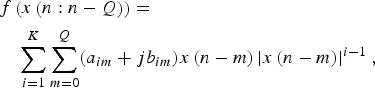 $$\eqalign{&f\left({x\left({n\colon n - Q} \right)} \right)= \cr & \quad \mathop \sum \limits_{i=1}^K \mathop \sum \limits_{m=0}^Q \lpar a_{im}+jb_{im} \rpar x\left({n - m} \right)\left\vert {x\left({n - m} \right)} \right\vert ^{i - 1}\comma}$$
where x(n:n − Q) is the [x(n), …, x(n − Q)]vector, K, Q and are the nonlinearity order, the memory depth and (a im + jb im) the complex parameters of the MP model, and x(n) is the complex envelope of the signal. In literature, no automated method for choosing the optimal order (K, Q) has been proposed. In the following, AIC and BIC will be discussed.
B) AIC and BIC
The concepts of AIC and BIC are based on minimizing the Kullback–Leibler (KL) distance, which measures the difference between two probability distributions. AIC and BIC belongs to a family of model order selection rules in which the KL measure is minimized. KL measure is defined as below [Reference Stoica and Selen9]:
 $$I\left({p_{1}0\comma \; PDF} \right)=E_{1}0 \left\{{{\rm ln}\lpar PDF\lpar {\bi y}\rpar } \right\}\comma$$
where y = y(1:N) is the output vector, N is the data length, p0 is the true PDF of the data, PDF(y) is the PDF of the model and E 0{.} is the expectation that is calculated over the true PDFp0(y). Since the model likelihood (PDF) is not available, assumptions have to be made, which will contribute in determining the model order selection criterion [Reference Stoica and Selen9].
Let us denote by θ = [a; b; σ2], the vector of model parameters, where σ, is the standard deviation of the error, e, and:
 $${\bi a}=\left[{a_{10} \; \ldots a_{1Q} a_{20} \ldots \; a_{im} \ldots \; a_{K0} \; \ldots a_{KQ} } \right]^T\comma$$
 $${\bi b}=\left[{b_{10} \; \ldots b_{1Q} b_{20} \ldots \; b_{im} \ldots \; b_{K0} \; \ldots b_{KQ} } \right]^T.$$
Let us denote by PDF(y, θ) the likelihood function of the output vector y, which depends on the parameter vector θ. The ML estimate of the parameters will be [Reference Stoica and Selen9]:
 $${\bi \hat \theta }=arg \lcub \mathop {max }\limits_{\bi \theta } \lcub \ln \lpar PDF({{\bi y}\comma \; {\bi \theta }} )\rpar \rcub \rcub .$$
Based on the Gaussianity of the residuals and by considering the fact that for complex data the data length will be 2N, the likelihood of the parameters for the nonlinear model follows the form below [Reference Stoica and Selen9]:
 $$PDF\left({{\bi y}\comma \; {\bi \theta }} \right)=\displaystyle{1 \over {\lpar 2\pi \rpar ^N \sigma ^{2N} }}{\rm exp}\left\{- \left({\displaystyle{\Vert {{\bi y} - f\lpar {\bi x}\rpar\Vert ^2 } \over {2\sigma ^2 }}} \right)\right\}.$$
Therefore, at the ML estimate of the parameters  ${\bi \hat \theta }$, the following relation is satisfied [Reference Stoica and Selen9]:
 $$- 2\ln \left({PDF\left({{\bi y}\comma \; {\bi \hat \theta }} \right)} \right)=constant+2Nln\left({\hat \sigma ^2 } \right).$$
In the definition of information criteria the fisher information matrix plays a critical role. The fisher information matrix is defined as:
 $${\bi J}=- E\left\{{\displaystyle{{\partial ^2 {\rm ln}\lpar PDF({{\bi y}\comma \; {\bi \theta }} )\rpar } \over {\partial {\bi \theta }\partial {\bi \theta }^T }}} \right\}\comma$$
where E{·} indicates the expectation. Using this matrix, the AIC has been defined as below [Reference Schwarz8]:
 $$AIC=- 2ln\left({PDF\left({y\comma \; \; \hat \theta } \right)} \right)+trace\left({{\bi J}_y \left({{\bi J}^{ - 1}+{\bi J}_y^{ - 1} } \right)} \right).$$
In which J is the fisher information matrix at the ML estimate of the parameters and equals to J y. In fact, J is the fisher matrix for a fictitious data with the same length and the same PDF but independent from y, from which the ML estimate of the parameters are obtained. Hence, AIC will take the following form [Reference Stoica and Selen9]:
 $$AIC = -2 \ln \left(PDF \left({\bi y}\comma \; {\bi \hat \theta} \right) \right) + 2p\comma$$
where p = 2K(Q + 1) + 1 is the number of parameters. Equation (8) can be reformulated as:
 $$AIC=2Nln\left({\hat \sigma ^2 } \right)+2p.$$
The effect of finite sample size on AIC can be considered as reported in [Reference Stoica and Selen9]:
 $$AIC = 2N\ln\left({\hat \sigma ^2 } \right)+\displaystyle{{2N} \over {2N - p - 1}}2p.$$
In [Reference Stoica and Selen9], it was shown that the PDF of  ${\bi \hat \theta }$ under regularity conditions is as follows:
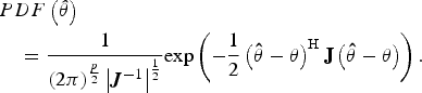 $$\eqalign{&PDF\left({{\bi \hat \theta }} \right)\cr & \quad=\displaystyle{1 \over {\lpar 2\pi \rpar ^{p\over2} \left\vert {{\bi J}^{ - 1} } \right\vert ^{1\over2} }}{\rm exp}\left({ - \displaystyle{1 \over 2}\left({{\bf \hat \theta } - {\bi \theta }} \right)^{\rm H} {\bf J}\left({{\bf \hat \theta } - {\bi \theta }} \right)} \right).}$$
In [Reference Stoica and Selen9], it was also shown that the unconditional PDF for the output signal will be:
 $$PDF \left({\bi y} \right)\approx PDF \left({{\bi y}\comma \; {\bi \hat \theta }} \right)PDF\lpar {\bi \hat \theta }\rpar \lpar 2\pi \rpar ^{p\over2} \left\vert {{\bi J}^{ - 1} } \right\vert ^{1\over2}.$$
and the BIC will be:
 $$BIC= - 2I\comma$$
where:
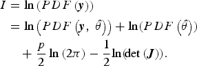 $$\eqalign{I& =\ln \left({PDF\left({\bi y} \right)} \right) \cr & = \ln \left({PDF\left({{\bi y}\comma \; {\bi \hat \theta }} \right)} \right)+\ln \lpar PDF\left({{\bi \hat \theta }} \right)\rpar \cr & \quad +\displaystyle{p \over 2}\ln \left({2\pi } \right)- \displaystyle{1 \over 2}{\rm ln}\lpar \!\det \left({\bi J} \right)\rpar.}$$
By considering that  $PDF\lpar {\bi \hat \theta }\rpar $ and
 ${p \over 2}\ln \left({2\pi } \right)$ are not function of N, and by considering high values of N, These two terms can be neglected. The BIC can then be approximated to:
 $$I \approx \ln \left({PDF\left({{\bi y}\comma \; {\bi \hat \theta }} \right)} \right)- \displaystyle{1 \over 2}\ln \left({\det \left({\bi J} \right)} \right).$$
The Fisher information matrix (J) was approximated in [Reference Stoica and Selen9] for large N as below:
 $$\ln \left({\det \left({\bi J} \right)} \right)=\ln \left({\det \left({N\displaystyle{1 \over N}{\bi J}} \right)} \right)\approx p\ln N+O\left(1 \right).$$
By using (6), (15), and (16), the expression of the BIC given in [Reference Stoica and Selen9] can be written as follows:
 $$BIC = 2N \ln \hat \sigma ^2+p\; ln\lpar N\rpar.$$
C) SISO system model order optimization
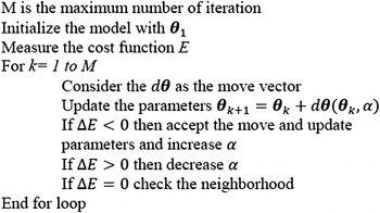
In the case of AIC and BIC for SISO systems, the criteria are convex based on practical observations and a convex optimization method such as gradient descent can be employed to find the optimum dimensions of the model. If the criterion is called by V N(θ) for the data length of N, and θ= [K, Q] then the idea of Gradient descent is to move in the direction of  $ - \displaystyle{{\partial V_N \lpar \theta \rpar } \over {\partial \theta }}$. However, our parameters (K, Q) are integer valued and the steps are discrete. The idea used in this paper consists of measuring the forward difference instead of the derivative and then rounding the value to the nearest integer to make the discrete step.
 $$d\theta=round\left({ - \alpha g\lpar V_N \left({\theta+1} \right)- V_N \left(\theta \right)\rpar } \right).$$
In which g(.) is a monotonic function and α is a scale parameter. If we define the forward difference vector as below:
 $$D=\left[{V_N \left({K+1} \right)- V_N \left(K \right)\semicolon \; V_N \left({Q+1} \right)- V_N \left(Q \right)} \right].$$
Then g(·) is defined as below:
 $$g\left(D \right)=\tanh \left({\displaystyle{{\left\vert D \right\vert } \over \Vert D\Vert}} \right)\left\vert {\log_{10} \left({1+\left\vert D \right\vert } \right)} \right\vert sign\left(D \right).$$
Herein ‖·‖ is the norm function. The term  $\displaystyle{{\vert D \vert} \over \Vert D \Vert}$ generates a normalized positive displacement. This function makes suitable steps for large and small D. For large D the logarithm term dominates and for small D the tanh(·) term dominates.
Fig. 1 shows the general algorithm of gradient descent. In the following section, the generalization of the criteria to the MIMO system will be studied.
Gradient descent algorithm.

III. MATRIX MEMORY POLYNOMIAL MODEL ORDER SELECTION IN MIMO TRANSMITTERS
A) MIMOAIC and MIMOBIC
The MMP technique has been developed to accurately model MIMO transmitters. The MMP model considers the effect of RF crosstalk between the two branches of the MIMO transmitter in addition to the transmitter nonlinearities [Reference Bassam, Helaoui and Ghannouchi12, Reference Amiri, Bassam, Helaoui and Ghannouchi13].
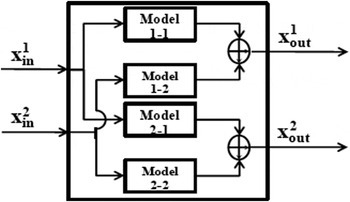
Figure 2 shows the architecture of the MMP model, in which the output of each branch is a function of both input signals as follows:
 $$y_i=f_{i1} \left({x_{in}^1 } \right)+f_{i2} \left({x_{in}^2 } \right)\; \; \semicolon \; \; i=1\comma \; 2\comma \;$$
where f ij(x) are nonlinear functions of the input signals, identified using both inputs and outputs of the MIMO transmitter.
MMP model for MIMO transmitters.

Using the modified Volterra series [Reference Arora, Huang and Hsieh14] for nonlinear functions, the expressions in (21) can be written as:
 $$f_{ij} \left({x\left(n \right)} \right)=\mathop \sum \limits_{l=1}^{K_{i\comma j} } \mathop \sum \limits_{m=0}^{Q_{i\comma j} } a_{lm\comma ij} x\lpar n - m\rpar \left\vert {x\lpar n - m\rpar } \right\vert ^{l - 1}\comma \;$$
where K i,j, Q i,j are the nonlinearity order and the memory depth of the MP used in (21) and a lm,ij is the complex coefficient.
Considering the fisher information matrices of each branch of the MIMO transmitter as J1 and J2 and the fisher information of the overall system as J, it was shown in Appendix A that the following approximation is valid:
 $$\ln\lpar \!\det \left({\bi J}_{\bi i} \right)= {\rm ln}\left( \!\det \left({{\bi J}_{i\comma 11} } \right)\right)\! +\ln \left({\det \left({{\bi J}_{i\comma 22} } \right)} \right)\semicolon \; for\; i=1\comma \; 2,$$
where Ji,11 and Ji,22 are matrices as defined in Apendix A.
Using (23), the BIC in (17) can be extended for the 2 × 2 MIMO system, and the new MIMOBIC is as follows:
 $$\eqalign{MIMOBIC_i & =2N\ln \left({\hat \sigma _i^2 } \right)\cr & \quad +\lpar p_1+1\rpar \ln\left(N \right)+p_2 \ln\left(N \right).}$$
In which p i = 2K i(Q i + 1).
By similar analysis it can be deduced that for the general MxP MIMO system the MIMOBIC can be generalized:
 $$MIMOBIC_i=2N\ln \left({\hat \sigma _i^2 } \right)+\left({1+\mathop \sum \limits_{j=1}^M p_j } \right){\rm ln}\lpar N\rpar {\rm }\comma \;$$
and for the AIC we will have:
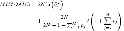 $$\eqalign{MIMOAIC_i & = 2N\ln\left({\hat \sigma _i^2 } \right) \cr & \quad + \displaystyle{{2N} \over {2N - 1 - \mathop \sum \nolimits_{j=1}^M p_j }}2\left({1+\mathop \sum \limits_{j=1}^M p_j } \right).}$$
B) MIMO system model order optimization
Obtaining the optimum degree for MMP models addressed in the paper necessitates minimizing MIMOAIC and MIMOBIC. Optimization of these integer variables (K i,j, Q i,j) using a double precision cost function can be cast as a mixed integer nonlinear programing.
In the case of MIMO system the situation is different. First, the problem may no longer be convex, since we have a larger number of parameters. Branch and bound, cutting plane, dynamic programing, implicit enumeration, and Lagrangian relaxation and simulated annealing were proposed in the literature [Reference Arora, Huang and Hsieh14, Reference Rutenbar15] to solve for this type of optimization. Simulated annealing was shown to be a powerful method for optimizing mixed nonlinear integer programming. In this paper, simulated annealing was used to optimize the MIMOAIC and MIMOBIC to obtain the optimum degrees and memory depths in the MP based models. Although the problem is not generally convex, the gradient descent algorithm was also applied. It was shown that the gradient descent could find a local optimum for which the performance of the estimated model is very close to the optimum value. This may come from the fact that the non-convexity of the problem is mostly due to the measurement setup accuracy. The gradient descent could find the local optimum in a few numbers of iterations and the results are provided to compare them with simulated annealing.
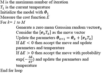
Simulated annealing first evaluates the cost function for an initial configuration. Then it perturbs the initial point with a random perturbation. Two cases will happen: the cost function will decrease which in this case, it will be considered as an acceptable movement. On the other hand if the cost function increases (ΔE) then it will be accepted with probability 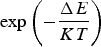 ${\rm exp}\left( - \displaystyle{{\Delta E} \over {KT}}\right) $. This property in simulated annealing avoids the algorithm to be trapped in local optimums. After each iteration, the temperature cools down with a scheme that limits uphill jumps at lower temperatures [Reference Rutenbar15]. The modified simulated annealing algorithm for integer parameters is explained in Fig. 3 [Reference Rutenbar15].
Simulated annealing algorithm.

For our case where the variables are integers, each move should be an integer too. Therefore, for the configuration update the following expression was used:
 $${\bi \theta }_{k+1}={\bi \theta }_k+\left[{{\bi e}_k T_k } \right]\comma \;$$
in which ek is a zero-mean vector Gaussian random variable normalized by its norm. After checking the bounds on the parameter vector again, the integer part of the new parameters is used. The initial temperatures were set to T 0 = 100 and the cooling scheme was selected to be T k = T 0 (0.95)k [Reference Rutenbar15].
IV. MEASUREMENT RESULTS
A) Measurement setup
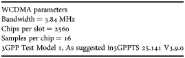
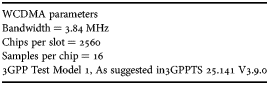
The excitation signals for system identification and evaluation are modulated wideband code division multiple access (WCDMA) with signal bandwidth of 3.84 MHz. Four different signals with different number of carriers, and therefore different bandwidths, denoted as 1, 11, 111, and 1111, have been used in the measurement validation. All these waveforms are 2-ms long and are sampled at the same frequency, 92.16 MHz. Table 1 summarizes the signal specifications for each carrier of these WCDMA signals. For modeling purposes 8000 points of the signals were used.
Modulated signals parameters.
Two different PAs, one class AB and one Doherty, are used in the course of measurement and performance evaluation.
The DUT in the class AB PA case is a cascade of a class A driver and a class AB PA biased at V gs = 9 V, Vds = 28 V. Both blocks are designed using the TF10107 LDMOS transistor. The output signals were attenuated and captured by vector signal analyzer (VSA89650S).
The DUT in the Doherty case is a high-power high-efficiency Doherty PA designed by LDMOS transistors provided by Powerwave Technologies. It has a peak power of 300 W and its small signal gain is 61 dB. The operating frequency is in the 2110–2170 MHz frequency band.
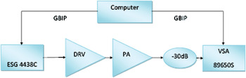
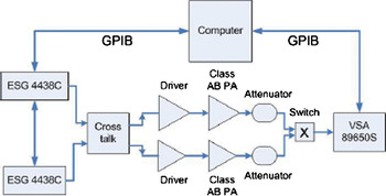
The measurement setup for the SISO and MIMO systems are shown in Figs. 4 and 5, respectively. For the SISO system in Fig. 4, it consists of a signal generator, a driver PA, PA, an attenuator and a vector signal analyzer (VSA) and for the MIMO case in Fig. 5, it consists of two signal generators (ESG4438C), cascade of two amplifiers (Class A and Class AB) and a VSA (89650S). The two signals are downloaded to the signal generators using GPIB interface.
SISO measurement setup.

MIMO measurement setup.

B) Results and discussion
The performance of AIC, BIC and the 2 × 2 MIMOAIC and MIMOBIC are examined and evaluated over single-branch and dual-branch PAs respectively.
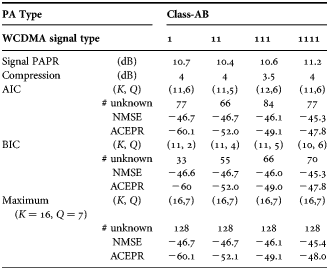
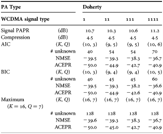
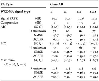
Tables 2 and 3 compare the performance of the MP model with the nonlinearity and memory depth order selection based on the AIC, BIC and maximum order of nonlinearity order of 16 and memory depth of 7 for class AB PA and Doherty PA. The maximum order is selected greater than what was reported in [Reference Isaksson, Wisell and Ronnow2].
NMSE and ACEPR mesurements for the models with optimal orders compared with higher order models for class AB PA.
NMSE and ACEPR mesurements of the the optimum models compared with the higher order models for Doherty PA.
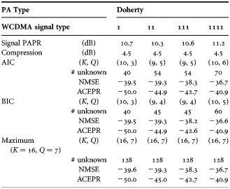
The calculated NMSE and adjacent channel error power ratio (ACEPR) metrics show that the performance of the model order selection based on BIC is very close to the optimum model order, but with less number of coefficients and processing complexity. The AIC criterion shows an over-fitting. The ACEPRs are calculated based on the following formula:
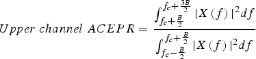 $$Upper\; channel\; ACEPR = \displaystyle{{\mathop \int \nolimits_{f_c+{B \over 2}}^{f_c+{3B \over 2}} \vert X \left(f \right)\vert ^2 df} \over {\mathop \int \nolimits_{f_c - {B \over 2}}^{f_c+ {B \over 2}} \vert X\left(f \right)\vert ^2 df}}$$
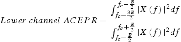 $$Lower\; channel\; ACEPR = \displaystyle{{\mathop \int \nolimits_{f_c - {3B \over 2}}^{f_c - {B \over 2}} \vert X\left(f \right)\vert ^2 df} \over {\mathop \int \nolimits_{f_c - {B \over 2}}^{f_c+ {B \over 2}} \vert X\left(f \right)\vert ^2 df}}$$
As can be seen from Tables 2 and 3, when the number of carriers increases the order decreases but the memory effect increases. The models with optimized orders using the BIC criterion showed linearity results very close to the models with maximum order (K = 16, Q = 7) while reducing the complexity considerably. Comparing to the AIC, this method estimates more efficient orders. The AIC most of the time over-estimates the orders. As can be seen from Tables 2 and 3, the same performance can be obtained by lower orders than what is estimated by BIC. This proves the validity of the new automated optimization approach.
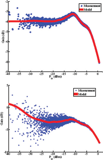
When the number of carriers increases, the higher bandwidth induces more memory effect. As can be seen form Fig. 6 the proposed optimization algorithm was able to predict this difference and same nonlinearity order but higher memory depth (10, 6) was obtained as the optimal model order for the four-carrier case.
Doherty PA AM/AM for (top) one carrier and (bottom) four carrier signals.

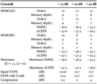
Similarly, Table-4 summarizes the results for MIMOAIC and MIMOBIC with the cross-over model of the dual-branch transmitter in the presence of 15, 20, and 30 dB nonlinear crosstalk [Reference Schwarz8]. The NMSE and ACEPR of the model selection based on MIMOAIC and MIMOBIC are compared with the maximum model order of nonlinearity order of 13 and memory depth of 6. It is clear that the optimization using MIMOBIC was able to obtain very similar linearity performance compared with the maximum order (K = 13, Q = 6), while reducing the complexity of the models considerably. In Table 4, nonlinearity order 1 and memory depth 1 are the nonlinearity order and memory depth of the model 1–1 and nonlinearity order 2 and memory depth 2 are the nonlinearity order and memory depth of the model 1–2 in Fig. 1.
NMSE of the optimum models compared to the higher order models for 2 × 2 MIMO systems.
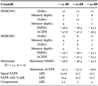
When the cross talk is low (−30 dB), the model behavior is close to SISO system. For the −15 dB crosstalk case more memory effect arises. The reason for lower nonlinearity order comes from the fact that a smoother curve is enough to fit the data in the case of −15 dB crosstalk but more dispersion is generated by the PAs, which requires higher memory order. The amount of AM–AM compression which is the difference in dB between input and output peak amplitudes is reported in Table 4.
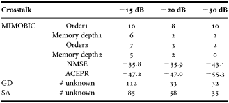
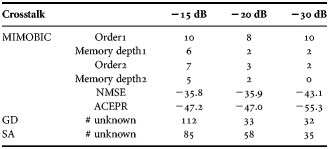
It is important to mention that not only the new optimization criteria is able to provide the user with an automated optimal order selection algorithm for any given amplifier, which guarantees a trade-off between linearity and complexity, it also allows us to use an optimization algorithm to reduce considerably the number of iterations of finding this optimal value. Indeed, by using Gradient descent in the SISO case the number of iterations was reduced from 128 to maximum 30. In the case of MIMO system, by using simulated annealing the number of iterations was reduced from 4096 to around 300 for the MIMO case. Using gradient descent for MIMO case shows that, although the global optimum could not be found, the performance of the local optimum is very close to the global optimum performance. The results of gradient descent are compared to simulated annealing in Table 5. This optimum search algorithm reduces the number of iterations to 50 from 4096. Therefore, it is recommended to use the gradient descent even in the MIMO case.
NMSE of the optimum models obtained using gradient descent for 2 × 2 MIMO systems.
V. CONCLUSION
In this paper, the application of information criteria, AIC, and BIC for model order selection in SISO and MIMO transmitters was presented. New criteria based on AIC and BIC, which includes model complexity as well as the NMSE metric, were proposed for MIMO dynamic nonlinear systems. To obtain the optimum model orders, two optimization algorithms were used for SISO and MIMO systems. Based on the convexity of the problem in the SISO case, a modified gradient descent algorithm was used. For the MIMO system since the problem is not generally convex and the number of parameters was higher, the simulated annealing algorithm was applied first and its performance was compared with the gradient descent algorithm. It was shown that the gradient descent in MIMO was able to obtain a local minimum with performance very close to the global optimum. It was also shown that AIC based criteria over-estimates the orders and is not efficient. Also, it was shown that with a negligible difference in NMSE and ACEPR, the model complexity is considerably reduced using BIC based criteria. As a conclusion, using the proposed criteria and the gradient descent optimum search algorithm, the optimum model order can be extracted automatically without the need for a complete order sweep. The number of iterations is therefore reduced from 128 to 30 for the SISO systems and from 4096 to 50 for the MIMO systems.
ACKNOWLEDGEMENT
This work was supported by the Alberta Innovate Technology Futures (AITF) Strategic Chair Program, the Natural Sciences and Engineering Research Council of Canada (NSERC), and the Canada Research Chairs (CRC) Program.
APPENDIX A
For the MIMO system, the error will be as below:
 $$e_i = y_i - f_{i{\bf 1}} \left({x_{\bf 1}} \right)+ f_{i{\bf 2}} \left({x_{\bf 2}} \right).$$
For each branch:
 $$PDF\left({{\bi y}_{\bi i} } \right)= PDF\left({{\bi y}_{\bi i}\comma \; {\bi \hat \theta }_{\bi i} } \right)PDF\left({{\bi \hat \theta }_{\bi i} } \right)\left({2\pi } \right)^{{p \over 2}} \left\vert {{\bi J}_{\bi i} ^{ - 1} } \right\vert ^{{1 \over 2}}\comma \;$$
which results in:
 $$I_i = \ln \left(PDF\left({\bi y}_{\bi i}\comma \; {\bi \hat \theta}_{\bi i} \right) \right) + \ln \lpar PDF\left({\bi \hat \theta}_{\bi i} \right)\rpar + \displaystyle{p \over 2} \ln \left(2\pi \right) - \displaystyle{1 \over 2} \ln \left(\det \left({\bi J}_{\bi i} \right) \right).$$
By approximating this equation the cost function will be:
 $$I_1 \approx \ln \left(PDF \left({\bi y}_1 \comma \; {\bi \hat \theta}_1 \right) \right) - \displaystyle{1 \over 2} \ln \left(\det \left({\bi J}_1 \right) \right).$$
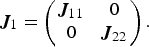
To obtain the Fisher information matrices J1 and J2 four cases should be considered. If we classify the coefficients to (11), (12) for the first branch and (22) and (22) for the second branch, then each Fisher information matrix will have four blocks. Among them there are two distinct cases:  $\displaystyle{\partial ^2 {\rm ln}\lpar PDF\left({\bi y}\comma \; {\bi \theta} \right)\rpar \over \partial a_{11im} \partial a_{11 jq}}\comma \; \displaystyle{\partial ^2 {\rm ln}\lpar PDF \left({\bi y}\comma \; {\bi \theta} \right)\rpar \over \partial a_{11 im} \partial a_{12 jq}}$. The first one will be the J11, which is the Fisher information matrix of the SISO system with input x 1 (n). The second one will be approximately zero because:
 $$\eqalign{\displaystyle{\partial ^2 \ln\lpar PDF \left({{\bi y}\comma \; {\bi \theta }} \right)\rpar \over \partial a_{11{im}} \partial a_{12 jq}} &= \displaystyle{1 \over 2\sigma^2} E\left\{\!\!{\mathop \sum \limits_{k=1}^N \!2x_1 \lpar k\rpar \left\vert {x_1 \lpar k\rpar} \right\vert^{i - 1} x_2 \lpar k\rpar^H \left\vert x_2 \lpar k\rpar \right\vert^{j - 1}}\!\! \right\} \cr &\approx 0.}$$
The overall Fisher information matrix for each branch will be as below:
 $${\bi J}_1 = \left(\matrix{{\bi J}_{11} & 0 \cr 0 & {\bi J}_{22}} \right).$$
The determinant of the overall fisher information matrix will be:
 $$\det \left({\bi J}_1 \right)= \det \left({\bi J}_{11} \right)\det \left({\bi J}_{22} \right).$$
By applying the logarithmic function to (A.7), we can write:
 $$\ln \left(\det \left({\bi J}_1 \right) \right)=\ln \left(\det \left({\bi J}_{11} \right) \right) + \ln \left(\det \left({\bi J}_{22} \right) \right).$$
Therefore, J2 will be as below:
 $$\ln \left(\det \left({\bi J}_2 \right) \right) = \ln \left(\det \left({\bi J}_{11} \right) \right) + \ln \left(\det \left({\bi J}_{22} \right) \right).$$
 Mehdi Vejdani Amiri received B.Sc. degree in Electrical engineering from the Sharif University of Technology of Iran in 2001 and received his M.Sc. degree in Communication Engineering from the Amirkabir University of Technology of Iran in 2004. He is now a Ph.D. candidate at the University of Calgary in the iRadio Lab. His main research interests are design and optimization of high power microwave power amplifiers, system identification and parameter estimation, stochastic processes and digital signal processing.
 Seyed Aidin Bassam (S'06, M'11) received his Ph.D. degree in electrical engineering from the University of Calgary, Calgary, AB, Canada in 2010. He was a postdoctoral researcher with iRadio laboratories at the University of Calgary 2010–2011. He is currently an RF system engineer at Qualcomm Technologies, San Diego, CA. His research interests are RF front-end design, digital predistortion and linearization techniques, and advanced digital signal processing techniques applicable to software defined radio, multi-standard and multi-band wireless communication systems.
 Mohamed Helaoui received (S'06-M'09) received his M.Sc. degree in communications and Information Technology from École Supérieure des Communications de Tunis, Tunisia, in 2003 and his Ph.D. degree in Electrical Engineering from the University of Calgary in 2008. He is currently an assistant professor at the Department of Electrical and Computer Engineering of the University of Calgary. His current research interests include digital signal processing, power efficiency enhancement for wireless transmitters, switching mode power amplifiers, and advanced transceiver design for software-defined radio and millimeter-wave applications. His research activities have led to over 60 publications and seven patents (pending). He is a member of the COMMTTAP chapter in the IEEE Southern Alberta section.
 Fadhel M. Ghannouchi is currently a Canada Research Chair/AITF Professor at Electrical and Computer Engineering Department of the Schulich School of Engineering of the University of Calgary and Director of Intelligent RF Radio Laboratory (www.iradio.ucalgary.ca). He held several invited positions at several academic and research institutions in Europe, North America, and Japan. He has provided consulting services to a number of microwave and wireless communications companies. His research interests are in the areas of microwave instrumentation and measurements, nonlinear modeling of microwave devices and communications systems, design of power, and spectrum-efficient microwave amplification systems and design of intelligent RF transceivers for wireless and satellite communications. His research activities led to over 500 publications and 14 US patents (6 pending). Professor Ghannouchi is a Fellow IEEE, Fellow IET and an Emeritus Distinguish Microwave Lecturer for IEEE-MTT Society.