


1. Introduction
Floods, earthquakes, and other catastrophic events occur infrequently, yet they can generate substantial financial losses. A sound understanding of both the frequency and the severity of such extremes is therefore essential for actuarial risk assessment. To model such phenomena, extreme value theory (EVT) provides a fundamental framework and is a standard tool in actuarial science and risk management (e.g., Embrechts et al., Reference Embrechts, Klüppelberg and Mikosch1997). In practice, however, risk assessments have traditionally relied primarily on point forecasts. By adopting predictive distributions, one obtains a more complete description of risk, and a growing body of literature has therefore focused on distributional approaches to uncertainty quantification (see, e.g., Benedetti, Reference Benedetti2010; Ruiz-Abellón et al., Reference Ruiz-Abellón, Fernández-Jiménez, Guillamón and Gabaldón2024; Klein et al., Reference Klein, Smith and Nott2023). Assessment of predictive distributions typically involves two complementary aspects: calibration, which examines whether predicted probabilities are statistically consistent with observed outcomes, and scoring rules, which provide a principled way to compare and rank different predictive distributions (Gneiting and Raftery, Reference Gneiting and Raftery2007; Gneiting et al., Reference Gneiting, Balabdaoui and Raftery2007). In actuarial applications, model selection rarely involves choosing between a clearly correct and a clearly incorrect specification. Practitioners typically face several competing models, so a data-driven ranking provides an objective and reproducible basis for pricing, reserving, and risk communication. In addition, the full ranking can guide the selection of alternative models when practical considerations such as interpretability, robustness, or regulatory constraints are taken into account. Accordingly, this paper proposes a method for ranking predictive distributions in the Fréchet domain based on proper scoring rules and normalized upper order statistics.
Because this approach relies on scoring-rule comparisons, it is crucial that the scoring rule remains proper, i.e.,
 \begin{align*}\mathbb{E}_{Y \sim F} [ S(F, Y) ] \geq \mathbb{E}_{Y \sim F} [ S(G, Y) ],\end{align*}
for all predictive distributions G, where
 $ S(\cdot, \cdot) $
denotes the scoring rule and
 $ Y \sim F $
represents the true data-generating distribution. Properness ensures that the forecaster is incentivized to issue their genuine predictive distribution (Gneiting and Raftery, Reference Gneiting and Raftery2007). The dangers of using improper scoring rules can be seen in Lerch et al. (Reference Lerch, Thorarinsdottir, Ravazzolo and Gneiting2017), which demonstrate how misassessment of extreme events can lead forecasters to issue predictions that are more extreme than they actually believe.
Against this background, there is a vast literature on the evaluation of predictive distributions with a focus on extreme events. One common approach is to employ weighted scoring rules, which allow greater emphasis to be placed on large observations, for example, by using a weight function of the form
 $ w(y) = \mathbf{1}\{y \geq t\} $
for some threshold t. Studies investigating proper weighted scoring rules include Gneiting and Ranjan (Reference Gneiting and Ranjan2011), Holzmann and Klar (Reference Holzmann and Klar2017), Allen (Reference Allen2024), Wessel et al. (Reference Wessel, Ferro, Evans and Kwasniok2025) and Ólafsdóttir et al. (Reference Ólafsdóttir, Rootzén and Bolin2024). In addition to their theoretical contributions, several of these studies provide empirical illustrations of how weighted scoring rules can be applied to evaluate tail performance. However, a central concern in this literature is whether expected scores can distinguish between different tail indices. Limitations of the CRPS in distinguishing tail behaviour are demonstrated in Taillardat et al. (Reference Taillardat, Fougères, Naveau and de Fondeville2023). More generally, Brehmer and Strokorb (Reference Brehmer and Strokorb2019) show in Theorem 5.4 that proper scoring rules cannot separate max-functionals in their framework. Since the tail index is a max-functional, a consequence of their result is that predictive distributions whose tail indices remain bounded away from the true tail index can attain expected scores arbitrarily close to the optimal expected score. Thus, differences in tail index need not imply a positive separation in expected score, and Allen et al. (Reference Allen, Koh, Segers and Ziegel2025) further strengthen this finding by showing that the limitation cannot be overcome by taking the maximum over multiple scoring rules. These results question the use of expected scores for assessing or comparing tail indices.
Our approach tackles this issue by changing the object on which the scoring rule is applied. Rather than seeking to separate tail indices through expected scores of the original predictive distributions, we base the comparison on normalized upper order statistics, leading to a limiting comparison between tail distributions. Let
 $Y_1,\ldots,Y_n$
denote the observations, with order statistics
 $Y_{n,1}\leq \cdots \leq Y_{n,n}$
. For a given number k of upper order statistics, the threshold is
 $Y_{n,n-k}$
, and each exceedance is evaluated relative to this threshold. Thus, the observations entering the score are
 \begin{align*} Y_{n,n-i+1}/Y_{n,n-k}, \qquad i=1,\ldots,k .\end{align*}
As the threshold increases, the distribution of the normalized exceedances converges, under suitable conditions, to a Pareto distribution determined entirely by the tail index. Consequently, in the limiting comparison, the tail index is no longer assessed as a max-functional of the original predictive distribution, but is instead the parameter of the distribution being scored.
This perspective is also closely related to weighted scoring rules. In Holzmann and Klar (Reference Holzmann and Klar2017), a study on how scoring rules can be transformed into weighted scoring rules while preserving propriety is provided. In particular, their Theorem 3 constructs weighted scoring rules by first normalizing the predictive distribution on the weighted region and then multiplying the resulting score by the weight function. With a deterministic threshold t, the corresponding analog in our setting is obtained by considering the rescaled variable
 $Y/t$
. On this scale, exceedances over t correspond exactly to the event
 $Y/t\geq 1$
, so the relevant weight is
 $w(y)=\mathbf{1}\{y\geq 1\}$
. The renormalized predictive distribution on this weighted region is then the conditional distribution of
 $Y/t$
given
 $Y\geq t$
. This connection also highlights where our approach departs from standard fixed-threshold weighted scoring rules. Weighted scoring rules can focus the evaluation on observations above a chosen threshold, but this alone does not provide a theoretical connection to the tail index. If the threshold is fixed, the score still evaluates a fixed part of the distribution, and there is no guarantee that this region reflects the limiting tail behavior. Hence, fixed-threshold weighting does not by itself resolve the difficulty that scoring-rule comparisons may fail to distinguish between different tail indices. The key feature of our approach is that the threshold is chosen as an intermediate order statistic and increases with the sample size. The score is thus evaluated on normalized exceedances in an increasingly extreme region, where the limiting distribution is determined by the tail index.
A related but distinct approach to tail-focused forecast evaluation is provided by tail calibration. For instance, Allen et al. (Reference Allen, Koh, Segers and Ziegel2025) introduce tail calibration as a tool for assessing calibration in the extremes and show that it can help distinguish between distributions with different tail behaviors. This perspective is complementary to the score-based ranking framework considered here and applies beyond the Fréchet domain.
Beyond model ranking, this paper also investigates scoring-rule optimization as a method for estimating the tail index. The idea is to choose the parameter value whose predictive distribution attains the largest empirical score. More precisely, let
 $\{F_\theta\,:\,\theta\in\Theta\}$
be a parametric class of distributions, let S be a strictly proper scoring rule, and let
 $(Y_1,\ldots,Y_n)$
be an i.i.d. sample. The scoring-rule estimator is then defined by
 \begin{align*} \hat{\theta}_S = \arg\max_{\theta\in\Theta} \sum_{i=1}^n S(F_\theta,Y_i).\end{align*}
Dawid et al. (Reference Dawid, Musio and Ventura2016) shows that, under regularity conditions, this estimator is consistent and asymptotically Gaussian. In addition, the associated estimating equation is shown to be unbiased. Under the equivalent loss orientation obtained by changing the sign of the score, this is commonly referred to as minimum scoring rule inference and falls within the broader framework of M-estimation (see, e.g., Huber and Ronchetti, Reference Huber and Ronchetti2009). Scoring-rule estimators have also found applications in the applied sciences, for instance in weather forecasting (Friederichs and Thorarinsdottir, Reference Friederichs and Thorarinsdottir2012), where CRPS is used. For a comprehensive review of scoring-rule inference, see Waghmare and Ziegel (Reference Waghmare and Ziegel2026).
Finally, we investigate the proposed framework through simulation studies and an empirical application. As part of the simulation study, we examine the effect of heterogeneous scaling. Such scale heterogeneity is not covered by the asymptotic theory in Section 4, but it is relevant in forecasting applications. We therefore include it as a simulation-based robustness check. In the extreme value theory literature, related non-identically distributed settings have been studied theoretically by Einmahl et al. (Reference Einmahl, de Haan and Zhou2016). For the empirical study, we use the usautoBI (USAutoBI) bodily injury claims data from the CASdatasets package in
 $\mathsf{R}$
. Five Pareto predictive distributions are compared and ranked using the proposed scoring-rule approach. We further consider two data partitions based on policyholder characteristics. While one split leads to the same ranking as in the full sample, the other results in a different ordering of the models, indicating that tail behavior varies across subpopulations.
In summary, our contributions are threefold: first, we propose a scoring-rule framework for tail-model ranking based on normalized upper order statistics; second, we provide asymptotic justification and show how score optimization yields a consistent tail-index estimator with Hill as a special case; and third, we illustrate the framework in simulation studies and in a real claim-severity application.
The paper is organized as follows. Section 2 introduces the core concepts from both the scoring rule and extreme value theory literature that are used throughout the paper. Section 3 introduces our proposed method, and Section 4 presents the main theoretical results. Section 5 investigates the finite-sample performance of our method through simulation studies, demonstrating promising results even for relatively small sample sizes. Finally, Section 6 applies the proposed scoring rule framework to a claim severity dataset.
2. Background and preliminaries
2.1. Proper scoring rules
Let
 $\mathcal{Y}=\mathbb{R}$
be equipped with the Borel
 $\sigma$
-algebra
 $\mathcal{A}$
, and let
 $\mathcal{F}$
denote a convex class of distribution functions on
 $\mathcal{Y}$
. Before defining the score function, we introduce the term quasi-integrable.
Definition 2.1 (
 $\mathcal{F}$
-quasi-integrable). f is quasi-integrable with respect to
 $F\in\mathcal{F}$
if it is
 $\mathcal{A}$
measurable and if either
 $f^+$
or
 $f^-$
has a real integral. f is
 $\mathcal{F}$
-quasi-integrable if it is quasi-integrable with respect to all
 $F\in \mathcal{F}$
.
With this setup, a scoring rule is defined as
Definition 2.2 (Scoring rule). Any
 $S\,:\, {\mathcal{F} \times \mathcal{Y}} \to \overline{\mathbb{R}}$
is a scoring rule if it is
 $\mathcal{F}$
-quasi-integrable for all
 ${F\in \mathcal{F}}$
.
With this notation, we write
 \begin{align} S(F,G)\,:\!=\,\mathbb{E}[S(F,{Y})]=\int S(F,y)\mathop{}\!\mathrm{d} G(y) \end{align}
where
 $F,G\in \mathcal{F}$
, and Y is a random variable with distribution function G.
A natural requirement of a scoring rule is that it is proper, which has the following definition.
Definition 2.3 (Proper scoring rule). Scoring rule S is proper relative to
 $\mathcal{F}$
if
 \begin{align*} S(G,G)\geq S(F,G) \end{align*}
for all
 $F,G\in \mathcal{F}$
. It is strictly proper if the inequality holds with equality if and only if
 $F=G$
.
Accordingly, using proper scoring rules incentivizes the forecaster to report their honest belief about the distribution. Therefore, the forecaster has no incentive to distort or strategically alter their forecast. Definition 2.3 is stated under the positive score orientation, meaning that larger score values correspond to better predictive performance.
Two widely used scoring rules are the logarithmic score (LogS) and the continuous ranked probability score (CRPS). The former is defined as
 \begin{align*}\mathrm{LogS}(F,y)\,:\!=\, \log {f}(y)\ \end{align*}
where f denotes the density of F. CRPS is defined as
 \begin{align*} CRPS(F,y)\,:\!=\,-\int_{-\infty}^{\infty}\left(F(x)-\mathbf{1}\{y\le x\}\right)^2\,dx.\end{align*}
CRPS can be viewed as a special case of the Energy score and, unlike the logarithmic score, it does not require the existence of a density. More generally, the Energy score with parameter
 $\beta \in (0,2)$
is defined as
 \begin{align*}ES_\beta(F,y)\,:\!=\,\frac12 \mathbb{E}|X-X'|^\beta - \mathbb{E}|X-y|^\beta,\end{align*}
where
 $X,X' \sim F$
are independent random variables. The CRPS coincides with
 $\mathrm{ES}_\beta$
for
 $\beta = 1$
. In this paper, we present results for the Energy score, of which the CRPS is a special case.
Both the logarithmic score and the Energy score with
 $\beta\in(0,2)$
are strictly proper; see, for example, Gneiting and Raftery (Reference Gneiting and Raftery2007).
2.2. Extreme value theory framework
A central result in extreme value theory is the Fisher–Tippett–Gnedenko theorem, which states that suitably normalized maxima converge in distribution to one of three possible types: Gumbel, Fréchet, or Weibull. These domains of attraction correspond to fundamentally different tail behaviors in the underlying distribution. See De Haan and Ferreira (Reference De Haan and Ferreira2006) for more information.
The Fréchet domain, also referred to as the heavy-tailed domain, encompasses distributions whose survival function decays according to a power law. Such distributions have infinite right endpoints and exhibit polynomially decreasing tails, implying that extreme events occur with non-negligible probability. Formally, a distribution function G is said to belong to the Fréchet domain of attraction if its survival function is regularly varying. That is, there exists a constant
 $\gamma \gt 0$
such that
 \begin{align}\lim_{t \to \infty} \frac{1 - G(tx)}{1 - G(t)} = x^{-1/\gamma}, \quad x \gt 0.\end{align}
The parameter
 $\gamma$
, called the tail index, quantifies the heaviness of the tail. When (2) holds, we say that the survival function
 $1-G$
is regularly varying with index
 $-1/\gamma$
, and write
 $1-G \in \mathcal{R}_{-1/\gamma}$
.
An equivalent characterization can be expressed in terms of the tail quantile function
 \begin{align*}U(x) = \inf\{ y \in \mathbb{R} \,:\, G(y) \ge 1 - 1/x \}, \qquad x \gt 1.\end{align*}
If
 $1-G \in \mathcal{R}_{-1/\gamma}$
, then the associated tail quantile function U is regularly varying with index
 $\gamma$
, that is,
 $U\in \mathcal{R}_{\gamma}$
In this paper, we let
 $(Y_1,Y_2, \ldots , Y_n)$
be an i.i.d. sample with common distribution function G. Throughout, we assume that
 $1-G\in \mathcal{R}_{-1/\gamma_G}$
. This implies that Y is in the Fréchet domain with tail index
 $\gamma_G$
. We now introduce the tail counterpart of G, which is given by
 \begin{align*}G^t(x)=\frac{G(tx)-G(t)}{1-G(t)}\quad \text{for $t\geq 1$.}\end{align*}
We denote
 $G^\circ$
as the limit distribution of
 $G^t$
and we call it the tail distribution.
 $Y^\circ$
denotes a random variable with distribution
 $G^\circ$
. As Y is in the Fréchet domain, we obtain
 \begin{align*}1-G^\circ(x)=\lim_{t\to \infty}1-G^t(x)=x^{-1/\gamma_G},\end{align*}
i.e.,
 $G^t$
converges to a Pareto distribution with parameter
 $1/\gamma_G$
.
3. Methodology for tail-model ranking and estimation
The purpose of this section is to turn the tail comparison described in the introduction into a computable score-based procedure. Rather than evaluating predictive distributions on the original sample space, we evaluate the score on normalized exceedances above a high threshold. The distribution used in the score is therefore a tail object associated with the predictive model. In the main implementation, this tail object is the Pareto limit distribution implied by the model, so the comparison directly targets differences in tail indices. More generally, the same framework can also be applied to finite-threshold tail counterparts when the aim is to assess tail fit above a fixed high threshold; see Remark 3.1.
Formally, for
 $F\in \mathcal{F}$
and any proper scoring rule, S, we have
 \begin{align*} \mathbb{E}[S(G^\circ, Y^\circ)]\geq \mathbb{E}[S(F, Y^\circ)],\end{align*}
where
 $Y^\circ \sim G^\circ$
. If S is a strictly proper scoring rule, we have equality if and only if
 $F=G^\circ$
. As
 $G^\circ$
is a Pareto distribution it is entirely described by the tail index,
 $\gamma_G$
, and hence
 \begin{align*} \mathbb{E}[S(G^\circ, Y^\circ)]=\mathbb{E}[S(F, Y^\circ)]\end{align*}
if and only if F is a Pareto distribution with the same tail index as
 $G^\circ$
. This highlights the distinction from the setting considered by Brehmer and Strokorb (Reference Brehmer and Strokorb2019). Their non-separability result concerns scoring the original predictive distributions, where distributions with tail indices bounded away from the true tail index can attain expected scores arbitrarily close to the optimum. In contrast, for the tail distributions considered here, under suitable conditions, tail indices bounded away from the true tail index are uniformly separated from the optimum in expected score. In particular, if the candidate tail indices are restricted to a compact set
 $\Gamma$
, then for every
 $\delta\gt0$
,
 \begin{align*}\mathbb{E}\!\left[S(G^\circ,Y^\circ)\right]\gt\sup_{\substack{\gamma\in\Gamma\\ |\gamma-\gamma_G|\geq\delta}}\mathbb{E}\!\left[S(F_\gamma,Y^\circ)\right],\end{align*}
provided that S is strictly proper and the expected score is continuous in
 $\gamma$
.
To connect this population comparison with sample quantities, note that
 \begin{align*}(V^t_{k,1}, V^t_{k,2}, \ldots , V^t_{k,k})\stackrel{d}{=} \left(\frac{Y_{n,n-k+1}}{Y_{n,n-k}}, \frac{Y_{n,n-k+2}}{Y_{n,n-k}}, \ldots , \frac{Y_{n,n}}{Y_{n,n-k}}\right)\Bigg| Y_{n,n-k}=t,\end{align*}
where
 $(V_i^t)_{i=1}^k$
are i.i.d. random variables with distribution
 $G^t$
and
 $Y_{n,1} \leq Y_{n,2} \leq \cdots \leq Y_{n,n}$
are the order statistics. As
 $G^t\to G^\circ$
when
 $t\to \infty$
, a natural estimator for
 $\mathbb{E}[S(F, Y^\circ)]$
is
 \begin{align} S_k(F)\,:\!=\,\frac{1}{k}\sum_{i=1}^k S\left(F, \frac{Y_{n,n-i+1}}{Y_{n,n-k}}\right). \end{align}
Consequently, this introduces an additional tuning parameter, k. It should be chosen small enough for
 $G^t$
to provide a good approximation to
 $G^\circ$
, yet large enough to ensure that the reduced sample remains sufficiently large for reliable inference. The EVT literature offers several methods for selecting k, most of which are based on identifying a range of values over which the estimator exhibits stability. In the simulation studies, we investigate this stability behavior.
In practice, we implement the procedure in the following way. First, choose a candidate set
 $\{F_1,\ldots,F_m\}$
and a grid
 $\mathcal{K}$
of values for k. Next, compute
 $S_k(F_j)$
for each j and
 $k\in\mathcal{K}$
. Then, identify a stability range
 $\mathcal{K}_{\mathrm{stab}}\subseteq \mathcal{K}$
, where the ordering is not driven by erratic local fluctuations. Finally, report the ranking based on both pointwise curves
 $k\mapsto S_k(F_j)$
and the average score over the stable range,
 \begin{align*}\bar S(F_j)\,:\!=\,\frac{1}{|\mathcal{K}_{\mathrm{stab}}|}\sum_{k\in\mathcal{K}_{\mathrm{stab}}} S_k(F_j).\end{align*}
This separates the statistical comparison (score level) from the threshold-sensitivity diagnostic (stability over k).
Remark 3.1. An important question is how to choose the distribution F used in the score. There are two natural choices, corresponding to different inferential targets.
The first choice is to use the tail limit distribution of F, that is, the Pareto distribution with tail index
 $\gamma$
implied by F. This is appropriate when the object of interest is the asymptotic tail index itself. In this formulation, two predictive distributions with the same tail index but different finite-threshold behaviour or different second-order properties have the same Pareto limit and are therefore asymptotically indistinguishable under the score.
The second choice is to use the finite-threshold tail counterpart
 $F^t$
, for instance with
 $t=Y_{n,n-k}$
. This retains information about the predictive distribution above a high but finite threshold and is therefore more appropriate when the objective is to assess finite-threshold tail fit. In this case, the score evaluates the conditional distribution of normalized exceedances above t, rather than only the limiting Pareto approximation.
In both cases, propriety should be understood relative to the transformed tail object being scored, not to the full predictive distribution on the original sample space.
Remark 3.2. A practical issue is the choice of scoring rule. Two of the most widely used scoring rules in the literature are LogS and CRPS. Notably, the LogS requires the predictive distribution to admit a density. This is unproblematic when F is specified as a Pareto distribution, for which the density is available in closed form. However, if one instead works with
 $F^t$
, evaluation of the corresponding density may be unavailable or computationally cumbersome. In such situations, the CRPS provides a convenient alternative, since it can be computed directly from the distribution function and therefore does not require density evaluation.
The same framework can also be used for tail-index estimation. In this case, we restrict attention to Pareto predictive distributions, since the objective is to estimate the tail index rather than to compare general predictive distributions. We propose a grid-search version of the estimator based on the empirical score in (3). Let
 $\Gamma \,:\!=\, [\gamma_L,\gamma_U]$
, with
 $0\lt\gamma_L\lt\gamma_U$
, and for each
 $\gamma \in \Gamma$
, let
 $F_\gamma$
denote the Pareto distribution with tail index
 $\gamma$
. For a given k, define
 \begin{align*}\widehat{\gamma}_{k}(S)\,:\!=\,\mathrm{argmax}_{\gamma\in\Gamma}\frac{1}{k}\sum_{i=1}^{k}S\left(F_\gamma,\frac{Y_{n,n-i+1}}{Y_{n,n-k}}\right).\end{align*}
In numerical implementations, the maximization over
 $\Gamma$
may be carried out over a finite grid.
4. Asymptotic results
In this section, we present consistency and asymptotic normality results for scoring rules based on the normalized order statistics introduced in Section 3. We also establish consistency for a tail-index estimator obtained by optimizing the empirical score.
To support the use of scoring rules for ranking tail models, it is important to establish their large-sample properties. Consistency is a fundamental requirement for any method aimed at tail evaluation, as it ensures that the correct model is identified in the limit. Although asymptotic normality is not strictly necessary, it is highly useful since it makes it possible to assess whether differences in scores between competing models are statistically significant.
4.1. Scoring with normalized upper order statistics
We begin with consistency. Consistency and asymptotic normality follow directly from Segers (Reference Segers2001) (Theorems 2.1 and 4.5). Here, the assumptions and theorem are restated in our notation. Although formulated below in terms of scoring rules, these results also apply to scoring functions
 $s(x,\cdot)$
, for any fixed action x, provided the stated regularity conditions are satisfied (see Gneiting, Reference Gneiting2011 for further discussion of scoring functions).
Assumption 4.1. Let
 $S\,:\,\mathcal{F} \times [1,\infty) \to \mathbb{R}$
be an a.e. continuous function for
 $F\in \mathcal{F}$
, and such that
 $|S(F,y)|\leq Ay^{(1-\delta)/\gamma_{G}}$
for some
 $A\gt0$
and
 $\delta\in (0,1)$
.
This assumption is mild and does not impose a substantial restriction, since commonly used scoring rules are typically continuous. The domination condition provides the necessary tail control.
Theorem 4.2. Let Assumption 4.1 hold. In addition, assume that
 $k,n \to \infty$
and
 $k/n \to 0$
. Then,
 \begin{align*}S_k(F)\;\rightarrow\;\mathbb{E}\!\left[S(F, Y^\circ)\right]\end{align*}
in probability, where
 $Y^\circ$
has distribution
 $G^\circ$
.
In practical terms, this result ensures that empirical tail scores converge to their population targets when k is chosen in the standard EVT regime.
We next turn to asymptotic normality, which follows as a direct consequence of Theorem 4.5 in Segers (Reference Segers2001). To establish this result, it is necessary to control the growth rate of k. We therefore introduce the following notation. Let
 $\xi \in \mathbb{R}$
, define the function
 $h_\xi \,:\, (0,\infty) \to \mathbb{R}$
by
 \begin{align*}h_\xi(x)= \int_1^x y^{\xi-1}\,dy=\begin{cases}\displaystyle \frac{x^\xi - 1}{\xi}, & \text{if } \xi \neq 0, \\[1ex]\log x, & \text{if } \xi = 0.\end{cases}\end{align*}
We may now restate Theorem 4.5 of Segers (Reference Segers2001) in our notation.
Theorem 4.3. Let G be a distribution function with tail quantile function U satisfying
 \begin{equation}\lim_{t \to \infty} \frac{U(tx)/U(t) - x^{\gamma_G}}{a(t)}= \pm x^{\gamma_G} h_{\xi}(x), \qquad x \ge 1,\end{equation}
for some
 $\gamma_G \gt 0$
,
 $\xi \le 0$
and
 $a \in \mathcal{R}_{\xi}$
satisfying
 $a(t) \to 0$
as
 $t \to \infty$
. Let
 $F\in\mathcal{F}$
be a fixed candidate distribution used in the score comparison. Let
 $S \,:\,\mathcal{F} \times [1,\infty) \to \mathbb{R}$
be an absolutely continuous function for
 $F\in \mathcal{F}$
with
 $\frac{\partial S}{\partial y}$
such that
 \begin{align*}\bigg|\frac{\partial S}{\partial y}\bigg| \le A y^{\rho-1}, \qquad y \ge 1,\end{align*}
for some
 $A \gt 0$
and some
 $\rho \lt (2\gamma_G)^{-1}$
. If k satisfies
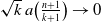 $\sqrt{k}\,a{\left(\frac{n+1}{k+1}\right)} \to 0$
when
 $k,n \to \infty$
and
 $k/n \to 0$
, then
 \begin{equation} \sqrt{k}\bigl(S_k(F) - \mathbb{E}[S(F,Y^\circ)]\bigr)\xrightarrow{d} \mathcal{N}\!\left(0,\operatorname{Var}(S(F,Y^\circ))\right).\end{equation}
The derivative condition is a regularity condition ensuring that the scoring rule behaves smoothly in the tail. As
 $y\mapsto S(F,y)$
is assumed absolute continuous, the condition also ensures that the variance exists. This normal approximation provides a direct basis for uncertainty quantification when comparing score levels across competing tail models.
The following corollary shows under which conditions Theorems 4.2 and 4.3 are applicable for LogS and ES.
Corollary 4.4. Let
 $F_\gamma$
denote a Pareto distribution with tail index
 $\gamma$
. Then:
-
1. The logarithmic score satisfies the assumptions of Theorems 4.2 and 4.3 for all
 $\gamma\gt0$
. Moreover,
\begin{align*} \operatorname{Var}(\mathrm{LogS}(F_\gamma,Y^\circ)) = \left(1+\frac{1}{\gamma}\right)^2\gamma_G^2 . \end{align*}
-
2. The Energy score satisfies the assumptions of Theorem 4.2 whenever
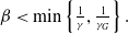
$ \beta \lt \min\left\{\frac{1}{\gamma},\frac{1}{\gamma_G}\right\}. $
It satisfies the assumptions of Theorem 4.3 whenever, in addition,
$ \beta \lt \frac{1}{2\gamma_G}. $
In particular, for
$\beta=1$
, corresponding to the CRPS, where
\begin{align*} \operatorname{Var}\!(\mathrm{ES}_1(F_\gamma,Y^\circ)) = \frac{1}{1-2\gamma_G} -\frac{2a}{1-(1+p)\gamma_G} +\frac{a^2}{1-2p\gamma_G} - \left( \frac{1}{1-\gamma_G} -\frac{a}{1-p\gamma_G} \right)^2, \end{align*}
$a=2\gamma/(\gamma-1)$
and
$p=1-1/\gamma$
, whenever the displayed moments are finite.






Proof. We verify the conditions separately for LogS and
 $\mathrm{ES}_\beta$
.
First consider LogS. If we denote the density of
 $F_\gamma$
as
 $f_\gamma$
, we have
 \begin{align*} \mathrm{LogS}(F_\gamma,y)=\log\!(\kern1.5pt f_\gamma(y))=\log(1/\gamma)-\left(\frac{1}{\gamma}+1\right)\log(y). \end{align*}
 $\mathrm{LogS}(F_\gamma,y)$
is absolute continuous for
 $y\gt1$
and for any
 $\delta\in (0,1)$
, it is dominated by
 $Ay^{(1-\delta)/\gamma_G}$
, where A is some constant. Further, we have
 \begin{align*} \frac{\partial \mathrm{LogS}}{\partial y}=-\left(\frac{1}{\gamma}+1\right)y^{-1} \end{align*}
For any
 $\rho \in (0,(2\gamma_G)^{-1})$
, this derivative is dominated by
 $Ay^{\rho-1}$
.
Next consider
 $\mathrm{ES}_\beta$
:
 \begin{align*}\mathrm{ES}_\beta(F_\gamma,y)&= {\frac{1}{2} \int_1^\infty\int_1^\infty |x - x'|^\beta \, \mathop{}\!\mathrm{d} F_\gamma(x) \mathop{}\!\mathrm{d} F_\gamma(x')-\int_1^\infty |x - y|^\beta \, \mathop{}\!\mathrm{d} F_\gamma(x)}.\end{align*}
For
 $y\geq 1$
, this expression is absolutely continuous. We first bound the first integral. For
 $\beta\lt\frac{1}{\gamma}$
, we have that
 \begin{align} \int_1^\infty |x - y|^\beta \, dF(x)&\leq A_1 \left(\int_1^y(y-1)^\beta x^{-1/\gamma -1}\mathop{}\!\mathrm{d}\kern1pt x + \int_y^\infty x^{\beta-1/\gamma-1}\mathop{}\!\mathrm{d}\kern1pt x\right) \\ &{\leq A_2 (y^{\beta}+y^{\beta-1/\gamma-1})}{\,\le A_3y^\beta}\nonumber\end{align}
for some constants
 $A_1,A_2,{A_3\gt0}$
. Hence, we can conclude that (6) is finite. Furthermore, for
 $\beta\lt\frac{1}{\gamma_G}$
, there exist some
 $\delta\in(0,1)$
and A such that it is dominated by
 $Ay^{(1-\delta)/\gamma_G}$
. Next, for the second integral, it is enough to verify finiteness since it does not depend on y:
 \begin{align*} &\int_1^\infty\int_1^\infty |x - x'|^\beta \, \mathop{}\!\mathrm{d} F_\gamma(x) \mathop{}\!\mathrm{d} F_\gamma(x')\nonumber\leq C_\beta\left(\int_1^\infty x^\beta\mathop{}\!\mathrm{d} F_\gamma(x)+\int_1^\infty (x')^{\beta}\mathop{}\!\mathrm{d} F_\gamma(x') \right)\end{align*}
for some
 $\beta$
dependent constant
 $C_\beta$
. Each of these integrals is finite for
 $\beta\lt\frac{1}{\gamma}$
. Hence, we can conclude that
 $\mathrm{ES}_\beta$
satisfies Assumption 4.1 for
 $\beta\lt\min\left\{1/\gamma,1/\gamma_G\right\}$
. Lastly, we have
 \begin{align*} \left|\frac{\partial \mathrm{ES}_\beta}{\partial y}\right|\leq {\beta \int_1^\infty |x-y|^{\beta-1}\mathop{}\!\mathrm{d} F(x)} \leq A_4y^{{\beta-1}}, \end{align*}
where
 $A_4$
is a constant. If
 $\beta \lt (2\gamma_G)^{-1}$
, choose
 $\rho$
with
 $\beta \lt \rho \lt (2\gamma_G)^{-1}$
. Since
 $y^{\beta-1} \leq y^{\rho-1}$
for
 $y \geq 1$
, the derivative condition is satisfied.
Therefore, both scoring rules satisfy the required conditions, which proves the claim.
This shows that the derivative condition mainly affects
 $\mathrm{ES}_\beta$
, where it imposes an additional restriction on the score parameter
 $\beta$
. For LogS, the condition is automatically satisfied and therefore imposes no further restriction.
Remark 4.5. We highlight two practical aspects that are relevant for applying the asymptotic results.
-
(i) The condition for
$ES_\beta$
depends on the true tail index
$\gamma_G$
, which is unknown in practice. This limitation should not be interpreted as excluding the Energy score for practical applications. For the common CRPS case
$\beta=1$
, the consistency condition is satisfied when the relevant tail indices are below one. This is a natural range in many insurance applications, since
$\gamma_G\lt1$
corresponds to finite mean claim sizes. The asymptotic normality condition is stronger and requires
$\gamma_G\lt1/2$
, corresponding to finite variance; this is more restrictive, but still not uncommon in insurance applications. The logarithmic score avoids this restriction and therefore provides a convenient default for tail-model ranking. -
(ii) The asymptotic variance in (5) depends on the unknown tail index
$\gamma_G$
. When an analytic variance formula is used, this parameter must therefore be replaced by a plug-in value, for instance a tail-index estimate. Alternatively, the variance may be estimated empirically.


Remark 4.6 The results in Theorems 4.2 and 4.3 are stated for an i.i.d. sample with a common tail distribution. Hence, they do not cover covariate-dependent or otherwise non-identically distributed predictive distributions. Extending the asymptotic theory to non-identically distributed predictive distributions would require additional assumptions on the conditional tail behavior, such as uniform regular variation or a common tail index across covariate values; see, for example, Bladt and Øhlenschlæ ger (Reference Bladt and Øhlenschlæger2025). The effect of heterogeneous scaling is investigated numerically in Section 5.2, but a detailed theoretical treatment of such extensions is beyond the scope of the present paper.
Taken together, Theorems 4.2–4.3 and Corollary 4.4 justify the following workflow: compute empirical tail scores over a range of (k), compare candidates by the score level, and use the normal approximation to assess whether observed score differences are practically meaningful.
4.2. Tail index estimation via score optimization
Beyond their use for ranking predictive distributions, we also investigate whether scoring rules can be employed for estimating the tail index. In this section, we assume that the predictive distribution is Pareto, denoted by
 $F_\gamma$
, where
 $\gamma$
is the candidate tail index. Let
 $\Gamma \,:\!=\, [\gamma_L,\gamma_U]$
, with
 $0\lt\gamma_L\lt\gamma_G\lt\gamma_U\lt\infty$
. For shorthand, define
 \begin{align*}S_k(\gamma)\,:\!=\,\frac{1}{k}\sum_{i=1}^k S\left(F_\gamma, \frac{Y_{n,n-i+1}}{Y_{n,n-k}}\right).\end{align*}
Restricting the predictive distributions to the Pareto family also gives a scoring-function interpretation of the procedure. In particular, any scoring rule S induces a scoring function for the tail index through
 \begin{align*}s(\gamma,y)\,:\!=\,S(F_\gamma,y).\end{align*}
Thus, the estimation procedure below may equivalently be viewed as optimization of an induced scoring function over
 $\gamma$
. Moreover, strict propriety of S implies that the expected induced score is uniquely maximized at the true tail index within the Pareto family.
The following theorem establishes consistency of the resulting tail-index estimator.
Theorem 4.7. Assume that S is continuous on
 $\Gamma\times[1,\infty)$
and a strictly proper scoring rule. Further assume Assumption 4.1 and that for
 $\gamma\in \Gamma$
, there exists a measurable function
 $D\,:\,[1,\infty)\to[0,\infty)$
such that
 \begin{align}\sup_{\gamma\in\Gamma}|S(F_\gamma,z)|\le D(z),\qquad z\ge 1,\end{align}
with
 $D(z)\le A z^{(1-\delta)/\gamma_G}$
for some
 $A\gt0$
and
 $\delta\in(0,1)$
. In particular,
 $E[|S(F_\gamma,Y^\circ)|]\lt\infty$
for all
 $\gamma\in\Gamma$
. Let
 $k\to\infty$
with
 $n/k\to\infty$
. Then,
 \begin{align} \hat{\gamma}_k(S)=\mathrm{argmax}_{\gamma\in \Gamma} \frac{1}{k}\sum_{i=1}^k S\left(F_\gamma, \frac{Y_{n,n-i+1}}{Y_{n,n-k}}\right) \xrightarrow{{\mathbb{P}}} \gamma_G. \end{align}
We first establish the following uniform convergence lemma.
Lemma 4.8. Assume the same conditions as in Theorem 4.7. Then, as
 $k\to\infty$
and
 $n/k\to\infty$
,
 \begin{align*}\sup_{\gamma\in\Gamma}\left|S_k(\gamma)-E[S(F_\gamma,Y^\circ)]\right|\xrightarrow{P}0 .\end{align*}
Proof of Lemma 4.8. Let
 \begin{align*} u(z,\theta,\tau)\,:\!=\, \sup_{\gamma{\in \Gamma}:|\gamma-\theta|\leq \tau}|S(F_\gamma,z)-S(F_\theta,z)|. \end{align*}
First, we argue that
 $z\mapsto u(z,\theta,\tau)$
is measurable. For fixed
 $\theta\in\Gamma$
and
 $\tau\gt0$
, let
 \begin{align*} \Gamma_{\theta,\tau}\,:\!=\,\{\gamma\in\Gamma\,:\,|\gamma-\theta|\le \tau\}. \end{align*}
Since
 $\Gamma_{\theta,\tau}$
is compact and
 $\gamma\mapsto S(F_\gamma,z)$
is continuous for each fixed z, the supremum over
 $\Gamma_{\theta,\tau}$
may be taken over any countable dense subset
 $Q_{\theta,\tau}\subset \Gamma_{\theta,\tau}$
. Hence,
 \begin{align*}u(z,\theta,\tau)=\sup_{\gamma\in Q_{\theta,\tau}}|S(F_\gamma,z)-S(F_\theta,z)|.\end{align*}
For each fixed
 $\gamma$
, the map
 $z\mapsto S(F_\gamma,z)$
is measurable, since S is a scoring rule. Therefore,
 $u(\cdot,\theta,\tau)$
is the pointwise supremum of countably many measurable functions and is consequently measurable.
By the continuity assumption of S, we have that
 $u(Y^\circ,\theta,\tau)\to 0$
for
 $\tau \to 0$
from above. Since S is dominated by D, by the triangle-inequality, we have that
 $u(Y^\circ,\theta,\tau)\leq 2D(Y^\circ)$
. Furthermore, since
 $Y^\circ$
is Pareto with tail index
 $\gamma_G$
, the bound
 $D(z)\leq A z^{(1-\delta)/\gamma_G}$
implies
 $E[D(Y^\circ)]\lt\infty$
. Hence, for a specific
 $\theta$
, we have by the dominated convergence theorem,
 $\mathbb{E} [u(Y^\circ,\theta,\tau)]\to 0$
as
 $\tau\to 0$
.
Now use compactness of the parameter space to cover it by finitely many balls
 $B(\theta_m,\tau_m)$
,
 $m=1,\dots,M$
, where
 $\theta_m\in \Gamma$
. By choosing M sufficiently large, we can ensure that for each ball
 \begin{align}\mu_m\,:\!=\,\mathbb{E}\big[u(Y^\circ,\theta_m,\tau_m)\big] \lt \varepsilon \end{align}
for any given
 $\varepsilon \gt 0$
. For a given
 $\gamma\in B_m$
we have
 \begin{align} |S_k(\gamma)-\mathbb{E}[S(F_\gamma,Y^\circ)]| &\leq |S_k(\gamma)-S_k(\theta_m)| \end{align}
 \begin{align} \qquad\qquad\qquad\qquad\qquad\qquad\qquad +|S_k(\theta_m)-\mathbb{E}[S(F_{\theta_m},Y^\circ)]| \end{align}
 \begin{align} \qquad\qquad\qquad\qquad\qquad\qquad\qquad\qquad\quad + |\mathbb{E}[S(F_{\theta_m},Y^\circ)]-\mathbb{E}[S(F_\gamma,Y^\circ)]| . \end{align}
For (10), note that
 \begin{align*} |S_k(\gamma)-S_k(\theta_m)| \leq \left|\frac{1}{k}\sum_{i=1}^k u\left(\frac{Y_{n,n-k+i}}{Y_{n,n-k}},\theta_m,\tau_m\right)-\mu_m\right|+\mu_m. \end{align*}
As argued earlier, we have
 \begin{align*} u(z,\theta_m,\tau_m) \leq 2Az^{(1-\delta)/\gamma_G}, \end{align*}
and by continuity of S and compactness of
 $\Gamma_{\theta,\tau}$
, we have that
 $z\mapsto u(z,\theta,\tau)$
is continuous. Hence, we can use Theorem 4.2 on
 $z\mapsto u(z,\theta_m,\tau_m)$
to conclude that
 \begin{align*} \frac{1}{k}\sum_{i=1}^k u\left(\frac{Y_{n,n-k+i}}{Y_{n,n-k}},\theta_m,\tau_m\right) \to \mu_m, \end{align*}
in probability. Since
 $\mu_m$
can be made arbitrarily small by selecting a large M, (10) can be made arbitrarily small. Likewise, (11) converges to 0 by Theorem 4.2, while (12) can be made arbitrarily small using
 \begin{align*} |\mathbb{E}[S(F_{\theta_m},Y^\circ)]-\mathbb{E}[S(F_\gamma,Y^\circ)]|\leq \mathbb{E}\big[u(Y^\circ,\theta_m,\tau_m)\big] \end{align*}
and (9).
Altogether, this shows that for any
 $\gamma \in B(\theta_m,\tau_m)$
, the quantity
 \begin{align*}|S_k(\gamma)-\mathbb{E}[S(F_\gamma,Y^\circ)]|\end{align*}
can be made arbitrarily small by choosing M sufficiently large. Since this holds for each of the finitely many balls in the cover, it also holds after taking the supremum over
 $\gamma \in \Gamma$
for M sufficiently large, which concludes the proof.
Proof of Theorem 4.7. By Lemma 4.8, we have
 \begin{align} \sup_{\gamma \in \Gamma}|S_k(\gamma)-\mathbb{E}[S(F_\gamma,Y^\circ)]|\xrightarrow{{\mathbb{P}}}0 \end{align}
as
 $k,n/k\to\infty$
. Using (13), we get that
 \begin{align} S_k(\hat{\gamma})\geq S_k(\gamma_G)\geq \mathbb{E}[S(F_{\gamma_G},Y^\circ)]-o_{\mathbb{P}}(1). \end{align}
Using (14) and (13), we get that
 \begin{align} \mathbb{E}[S(F_{\gamma_G},Y^\circ)] - \mathbb{E}[S(F_{\hat{\gamma}},Y^\circ)] \leq S_k(\hat{\gamma})+o_{\mathbb{P}}(1)-\mathbb{E}[S(F_{\hat{\gamma}},Y^\circ)] \end{align}
 \begin{align} \qquad\qquad\qquad\qquad\qquad\qquad\qquad\qquad \leq \sup_{\gamma \in \Gamma} |S_k(\gamma)-\mathbb{E}[S(F_\gamma,Y^\circ)]|+o_{\mathbb{P}}(1) \xrightarrow{{\mathbb{P}}}0 \end{align}
as
 $k,n/k\to \infty$
. Since
 $Y^\circ\sim F_{\gamma_G}$
, strict propriety of S implies that
 \begin{align*}\mathbb{E}[S(F_\gamma,Y^\circ)]\lt\mathbb{E}[S(F_{\gamma_G},Y^\circ)]\end{align*}
whenever
 $F_\gamma\neq F_{\gamma_G}$
. By identifiability of the Pareto family, this holds for every
 $\gamma\neq\gamma_G$
. Moreover, the map
 $\gamma\mapsto \mathbb{E}[S(F_\gamma,Y^\circ)]$
is continuous by dominated convergence. Hence, for every
 $\varepsilon\gt0$
, the compact set
 $\{\gamma\in\Gamma:|\gamma-\gamma_G|\geq\varepsilon\}$
admits a maximizer. Since this maximizer differs from
 $\gamma_G$
, we obtain
 \begin{align*}\sup_{\gamma:|\gamma-\gamma_G|\geq\varepsilon}\mathbb{E}[S(F_\gamma,Y^\circ)]\lt\mathbb{E}[S(F_{\gamma_G},Y^\circ)].\end{align*}
Hence, for every
 $\varepsilon\gt0$
, there exists an
 $\eta\gt0$
such that
 \begin{align*} \mathbb{E}[S(F_{\hat{\gamma}},Y^\circ)]\lt\mathbb{E}[S(F_{\gamma_G},Y^\circ)]-\eta \quad \text{when } |\hat\gamma-\gamma_G|\geq \varepsilon . \end{align*}
Therefore,
 \begin{align*} \{|\hat{\gamma}-\gamma_G|\geq \varepsilon\} \subset\{\mathbb{E}[S(F_{\hat{\gamma}},Y^\circ)]\lt\mathbb{E}[S(F_{\gamma_G},Y^\circ)]-\eta\}, \end{align*}
and as the right-hand side converges to 0 in probability by (16), the left-hand side also converges to 0.
When the empirical maximizer lies on the boundary of
 $\Gamma$
, the estimate is a boundary optimum induced by the restricted parameter space. It may therefore reflect that the unconstrained empirical optimum lies outside
 $\Gamma$
, so such a solution should be interpreted with care rather than as direct evidence that the true tail index coincides with the boundary point. For the logarithmic score, this boundary effect can be described explicitly: the unconstrained estimator is the Hill estimator, while the constrained estimator over
 $\Gamma$
is its projection onto
 $\Gamma$
.
Remark 4.9. Let
 $F_\gamma^\circ$
denote the Pareto distribution on
 $[1,\infty)$
with tail index
 $\gamma$
, and let
 \begin{align*}\widehat\gamma_H=\frac{1}{k}\sum_{i=1}^k\log\left(\frac{Y_{n,n-i+1}}{Y_{n,n-k}}\right)\end{align*}
denote the Hill estimator. Then, the logarithmic-score estimator over the parameter space
 $\Gamma$
is the projection of the Hill estimator onto this interval, i.e.,
 \begin{align*}\mathop{\mathrm{argmax}}\limits_{\gamma\in\Gamma}\frac{1}{k}\sum_{i=1}^k\log\left[f_\gamma^\circ\left(\frac{Y_{n,n-i+1}}{Y_{n,n-k}}\right)\right]=\Pi_{\Gamma}(\widehat\gamma_H),\end{align*}
where
 $\Pi_{\Gamma}(x)=\min\{\gamma_U,\max\{\gamma_L,x\}\}$
. In particular, if
 $\widehat\gamma_H\in\Gamma$
, then the logarithmic-score estimator coincides with the Hill estimator.
Remark 4.10. Segers (Reference Segers2001) shows that, under mild conditions on h, the estimator of the form
 \begin{align*}\frac{1}{k}\sum_{i=1}^k h\!\left(\frac{Y_{n,n-i+1}}{Y_{n,n-k}}\right)\end{align*}
attains the smallest asymptotic variance when
 $h=\log$
. This suggests that it is inherently difficult to construct a scoring-rule-based estimator
 $\hat{\gamma}_k$
that outperforms the Hill estimator in terms of asymptotic efficiency.
The following corollary verifies the assumptions of Theorem 4.7 for LogS and
 $ES_\beta$
.
Corollary 4.11. The assumptions of Theorem 4.7 are satisfied when
-
1. using LogS for all
$\gamma\gt0$
; -
2. using
$ES_\beta$
with
$\beta\lt\frac{1}{\gamma_U}$
.


For the second statement,
 $\beta\lt1/\gamma_U$
guarantees the required bound simultaneously for all
 $\gamma\in\Gamma$
. For a fixed candidate
 $\gamma$
, however, the weaker condition
 $\beta\lt1/\gamma$
may suffice.
Proof. For LogS, the map
 $(\gamma,z)\mapsto \mathrm{LogS}(F_\gamma,z)$
is continuous on
 $\Gamma\times[1,\infty)$
, and LogS is strictly proper. Moreover, the calculations in the proof of Corollary 4.4 show that
 \begin{align*}\sup_{\gamma\in\Gamma}|\mathrm{LogS}(F_\gamma,z)|\leq Az^{(1-\delta)/\gamma_G}.\end{align*}
Hence, the assumptions of Theorem 4.7 are satisfied for LogS.
For
 $ES_\beta$
, the map
 $(\gamma,z)\mapsto ES_\beta(F_\gamma,z)$
is continuous on
 $\Gamma\times [1,\infty)$
, and
 $ES_\beta$
is strictly proper. By the calculations in the proof of Corollary 4.4, for each fixed
 $\gamma$
with
 $\beta\lt1/\gamma$
, there exists a constant
 $C_\gamma\gt0$
such that
 \begin{align*} |ES_\beta(F_\gamma,z)|\leq C_\gamma(1+z^\beta).\end{align*}
Since
 $\beta\lt1/\gamma_U$
, we have
 $\beta\lt1/\gamma$
for every
 $\gamma\in\Gamma$
. Moreover, it is seen from the calculations in the proof of Corollary 4.4 that the constant
 $C_\gamma$
can be chosen as a continuous function of
 $\gamma$
. Since
 $\Gamma$
is compact,
 $C(\gamma)$
is bounded on
 $\Gamma$
. Hence, there exists
 $C\gt0$
such that
 \begin{align*} \sup_{\gamma\in\Gamma}|ES_\beta(F_\gamma,z)|\leq C(1+z^\beta).\end{align*}
 \begin{align*}|ES_\beta(F_\gamma,z)|\leq C_\gamma\left(1+z^\beta\right).\end{align*}
Since
 $\gamma_G\in\Gamma$
, the condition
 $\beta\lt1/\gamma_U$
implies
 $\beta\lt1/\gamma_G$
. Hence, we may choose
 $\delta\in(0,1)$
such that
 \begin{align*}\beta\lt\frac{1-\delta}{\gamma_G}.\end{align*}
It follows that for
 $z\geq 1$
,
 \begin{align*}C(1+z^\beta)\leq A z^{(1-\delta)/\gamma_G}\end{align*}
for some
 $A\gt0$
. Therefore, the uniform envelope condition in Theorem 4.7 is satisfied, and the result follows.
Remark 4.12. Corollary 4.11 gives a uniform sufficient condition for the Energy-score estimator over the parameter interval
 $\Gamma=[\gamma_L,\gamma_U]$
. For
 $ES_\beta$
, this condition requires
 $\beta \lt 1/\gamma_U$
. Thus, allowing larger values of
 $\gamma_U$
forces smaller choices of
 $\beta$
. In the CRPS case,
 $\beta=1$
, this corresponds to the condition
 $\gamma_U \lt 1$
. Hence, for score-based tail-index estimation, the Energy-score estimator is most natural when the parameter interval can be chosen so that commonly used values of
 $\beta$
remain admissible.
5. Simulation study
This section explores our theoretical results through three simulation studies. First, we investigate the ability of (3) to differentiate between tail indices. Next, we assess robustness when the scaling varies systematically across observations. Lastly, we examine the finite-sample behavior of
 $\widehat{\gamma}_{k}(S)$
for Energy-score-based tail-index estimation, compared with the classical Hill estimator.
Across all studies, the primary diagnostic is stability of the score or estimator curve over k: reliable behavior should persist over a non-negligible k-range rather than at isolated grid points.
5.1. Ranking tail models: baseline setting
In the baseline setting, the purpose of the simulation study is to assess how well a LogS rule can identify the true tail index of a heavy-tailed distribution and how this depends on the threshold level and the sample size.
Samples of size
 $n \in \{10^3, 10^4, 10^5\}$
are generated from heavy-tailed distributions with true tail index
 $\gamma_G = 1$
. We consider two parametric families of distributions, namely the Fréchet and the Burr distributions. The Fréchet distribution is specified by the distribution function
 \begin{align*}F(x) = \exp\!\left(-x^{-s}\right), \qquad x \gt 0,\end{align*}
where the shape parameter is set to
 $s = 1/\gamma_G$
. The Burr distribution is given by
 \begin{align*}F(x) = 1 - \bigl(1 + x^{c}\bigr)^{-t}, \qquad x \gt 0,\end{align*}
with shape parameters chosen as
 $c = 1/\gamma_G$
and
 $t = 1$
. With these parameterizations, both distributions are characterized by the same tail index
 $\gamma_G$
.
Empirical logarithmic scores in (3) (vertical axis) plotted against the number of upper order statistics k (horizontal axis) for candidate tail indices
 $\gamma \in \{0.8, 1, 1.2, 1.5\}$
. Left panels use Fréchet data-generating distributions, right panels use Burr distributions, and rows correspond to
 $n=10^3,10^4,10^5$
. Higher curves indicate better tail fit; the true value is
 $\gamma_G=1$
.

Figure 1. Long description
The image contains six line graphs. Panel A shows Fréchet DGP with n = 10^3, Panel B shows Burr DGP with n = 10^3, Panel C shows Fréchet DGP with n = 10^4, Panel D shows Burr DGP with n = 10^4, Panel E shows Fréchet DGP with n = 10^5, and Panel F shows Burr DGP with n = 10^5. Each graph plots empirical logarithmic scores (vertical axis) against the number of upper order statistics k (horizontal axis) for candidate tail indices γ = 0.8, γ = 1, γ = 1.2, and γ = 1.5. Higher curves indicate better tail fit, with the true value being γ = 1.
Within each sample, the threshold parameter k ranges from 50 to
 $n/4$
and is evaluated on an evenly spaced grid of 100 points. For each value of k, four logarithmic scores are computed by taking F to be a Pareto distribution with tail index
 \begin{align*}\gamma \in \{0.8,\,1,\,1.2,\,1.5\}.\end{align*}
Using this setup, the empirical criterion is computed via (3). In Figure 1, the resulting scores of a single realization are plotted as functions of k, with one curve corresponding to each value of
 $\gamma$
. If the scoring rule is well aligned with the true tail behavior, the candidate value
 $\gamma = \gamma_G = 1$
should yield the highest log score across a broad range of k. To formalize this comparison, for each fixed k, the candidate values are ranked according to their empirical logarithmic scores. In particular, the highest-ranked value is
 \begin{align*} \mathop{\mathrm{argmax}}\limits_{\gamma \in \{0.8,1,1.2,1.5\}} \mathrm{LogS}_k(\gamma),\end{align*}
with the remaining candidates ordered according to their corresponding scores. For the smaller sample sizes
 $n=10^3$
and
 $n=10^4$
, and in particular for the Burr model, the curve corresponding to
 $\gamma=1$
is not systematically above the competing curves; instead, the candidate values
 $\gamma=0.8$
and
 $\gamma=1.2$
often attain similar or larger scores over substantial ranges of k. By contrast, clearer signals appear in the remaining cases, especially for
 $n=10^5$
and for the Fréchet model, where the curve corresponding to
 $\gamma=1$
tends to dominate over a noticeable region of smaller k. This pattern is consistent with the expected bias-variance trade-off in tail inference: with larger n, a wider lower-k region supports stable discrimination of the correct tail index. This visual impression is further supported by a Monte Carlo experiment reported in Figure 2. For each configuration, 100 independent samples are generated, and the empirical logarithmic score is computed for the candidate values
 $\gamma \in \{0.8,1,1.2,1.5\}$
across the same range of thresholds. For each value of
 $k/n$
, we record whether the score is maximized at the true value
 $\gamma=1$
and plot the resulting proportion of such occurrences across the simulations. In both the Fréchet and Burr cases, when
 $n=10^3$
, there is no clear tendency for the proportion to approach one as
 $k/n$
goes to 0. As the sample size increases, however, the proportion rises in both models. For Fréchet data-generating distributions, this increase is particularly strong. When
 $n=10^5$
, the proportion is equal to one across the entire range of
 $k/n$
, indicating that the correct tail index is almost always selected. In the Burr case, the increase is observed only for smaller values of k/n, indicating that the correct tail index is consistently favored only further into the tail.
Proportion of simulations (based on 100 Monte Carlo replications) in which the empirical logarithmic score in (3) is maximized at the true tail index
 $\gamma=1$
among candidate values
 $\gamma \in \{0.8, 1, 1.2, 1.5\}$
, plotted against the relative number of upper order statistics
 $k/n$
. The left plot uses Fréchet data-generating distributions and the right plot uses Burr distributions. Curves correspond to sample sizes
 $n=10^3,10^4,10^5$
. Higher values indicate that the logarithmic score more frequently identifies the true tail index.

It should be noted that both the Fréchet and Burr samples are evaluated against Pareto limit distributions. Although
 $\gamma=1$
gives the correct asymptotic tail index in both cases, finite-threshold exceedances are not exactly Pareto, so larger values of
 $k/n$
may still reflect pre-asymptotic distributional features. Hence, it is expected that the correct tail-index signal is clearest for smaller values of
 $k/n$
.
5.2. Ranking tail models under heterogeneous scaling
A practically relevant situation is one in which the observations are not identically distributed. For example, covariates may affect the scale of the underlying distribution. Although such settings go beyond the asymptotic theory developed in Section 4, we include the following simulation experiment to examine the robustness of the proposed approach under systematic scale variation. Specifically, we simulate independent baseline heavy-tailed variables Z from Burr and Fréchet distributions and multiply each realization by a scaling factor. That is,
 \begin{align*}Y_i = X_i Z_i .\end{align*}
We follow the same setup as in Section 5.1 to generate the baseline heavy-tailed variable Z. We consider two different structures for the scaling factors X:
-
(i)
$X_i^1={1+}\frac{i}{n}$
. -
(ii)
$X_i^2=1.5+0.5\sin\!\left(6\frac{i}{n}\pi\right)$
.


Both scaling structures imply that
 $X_i\in[1,2]$
. These two structures represent qualitatively different forms of scale heterogeneity and should be viewed as simple heuristic stress tests. They are chosen to separate two effects that may arise in practice: persistent changes in scale and recurrent scale fluctuations. The monotone structure captures the former, with the largest scale occurring only at the end of the sample. The periodic structure captures the latter, producing repeated high-scale regions so that several parts of the sample contain observations with the largest scale.
Importantly, in this simulation design the tail index is constant across all observations. The only source of heterogeneity arises from the scaling component. Consequently, the tail heaviness of the distribution remains unchanged, while only the scale varies across i. Under this setup, the model corresponding to
 $\gamma = 1$
correctly specifies the tail index of the data-generating process. Therefore, we would expect the logarithmic score (LogS) to attain its highest value at
 $\gamma = 1$
.
Figures 3 and 4 present the results of a single realization, while Figure 5 reports the proportion results. The figures are constructed in the same manner as those in the previous section and are therefore not described in further detail. The same k-grid and candidate set as in Section 5.1 are used, so changes in behavior can be attributed to the scaling mechanism. Even in the presence of heterogeneous scaling, the qualitative conclusions of Section 5.1 remain valid. In particular, the logarithmic score continues to favor the correct tail index for sufficiently large sample sizes and appropriate choices of k, and the most reliable inference is still concentrated in a stable lower-k region.
Empirical logarithmic scores (vertical axis) versus k (horizontal axis) for Fréchet baseline samples with heterogeneous scaling,
 $Y_i=X_iZ_i$
, where
 $Z_i$
has tail index
 $\gamma_G=1$
. Candidate tail indices are
 $\gamma \in \{0.8, 1, 1.2, 1.5\}$
. Left panels use
 $X_i^1={1+}i/n$
, right panels use
 $X_i^2=1.5+0.5\sin(6\pi i/n)$
, and rows correspond to
 $n=10^3,10^4,10^5$
.

Figure 3. Long description
The image contains six line graphs. Each graph shows empirical logarithmic scores on the vertical axis and k on the horizontal axis. The graphs compare different tail indices (gamma values: 0.8, 1, 1.2, 1.5) for Fréchet baseline samples with heterogeneous scaling. Panel A shows linear scaling with n = 10^3. Panel B shows sinusoidal scaling with n = 10^3. Panel C shows linear scaling with n = 10^4. Panel D shows sinusoidal scaling with n = 10^4. Panel E shows linear scaling with n = 10^5. Panel F shows sinusoidal scaling with n = 10^5. Each graph displays multiple lines representing different gamma values, illustrating how the empirical logarithmic scores vary with k for each scaling method and sample size.
Empirical logarithmic scores (vertical axis) versus k (horizontal axis) for Burr baseline samples with heterogeneous scaling,
 $Y_i=X_iZ_i$
, where
 $Z_i$
has tail index
 $\gamma_G=1$
. Candidate tail indices are
 $\gamma \in \{0.8, 1, 1.2, 1.5\}$
. Left panels use
 $X_i^1={1+}i/n$
, right panels use
 $X_i^2=1.5+0.5\sin(6\pi i/n)$
, and rows correspond to
 $n=10^3,10^4,10^5$
.

Proportion of simulations (based on 100 Monte Carlo replications) in which the empirical logarithmic score in (3) is maximized at the true tail index
 $\gamma=1$
among candidate values
 $\gamma \in \{0.8, 1, 1.2, 1.5\}$
, plotted against the relative number of upper order statistics
 $k/n$
. The top panels correspond to Fréchet data-generating distributions and the bottom panels to Burr distributions. The left panels use a linearly varying scale, while the right panels use a sinusoidally varying scale. Curves correspond to sample sizes
 $n=10^3,10^4,10^5$
. Higher values indicate that the logarithmic score more frequently identifies the true tail index.

Figure 5. Long description
Four line graphs compare the proportion of simulations where the empirical logarithmic score is maximized at the true tail index among candidate values against the relative number of upper order statistics. Panel A: Fréchet DGP, Linear scaling Xi = Xi^1. The y-axis represents the proportion, ranging from 0 to 1, and the x-axis represents the relative number of upper order statistics, ranging from 0.05 to 0.25. Panel B: Fréchet DGP, Sinusoidal scaling Xi = Xi^2. The y-axis represents the proportion, ranging from 0 to 1, and the x-axis represents the relative number of upper order statistics, ranging from 0.05 to 0.25. Panel C: Burr DGP, Linear scaling Xi = Xi^1. The y-axis represents the proportion, ranging from 0 to 1, and the x-axis represents the relative number of upper order statistics, ranging from 0.05 to 0.25. Panel D: Burr DGP, Sinusoidal scaling Xi = Xi^2. The y-axis represents the proportion, ranging from 0 to 1, and the x-axis represents the relative number of upper order statistics, ranging from 0.05 to 0.25. Each panel includes three lines representing different sample sizes: n = 1000, n = 10000, and n = 1e+05. Higher values indicate that the logarithmic score more frequently identifies the true tail index.
5.3. Finite-sample performance of score-optimization estimators
We now examine the finite-sample behavior of tail-index estimators based on the Energy score,
 $\hat{\gamma}_k(ES_\beta)$
, to illustrate the finite-sample behavior of Energy-score-based estimation. Their performance is compared with that of the classical Hill estimator over a range of tail indices. Recall that the parameter
 $\beta$
must satisfy
 $\beta \lt 1/\gamma^U$
.
Samples of size
 $n = 10^4$
are generated from Fréchet distributions. Companion Burr runs were also conducted but are not shown, as they display the same qualitative sensitivity in k and
 $\beta$
and were omitted for brevity. As in the previous simulation studies, the remaining parameters are chosen analogously. The number of upper order statistics k is varied over 25 equally spaced values between 50 and
 $n/4$
. The Energy score was evaluated over the compact parameter space
 \begin{align*}\Gamma=[\gamma_L,\gamma_U]=[\,0.8\gamma_G,\,2\gamma_G\,],\end{align*}
using a grid of 150 equidistant candidate values. The interval is a heuristic choice, included to contain the true value while also allowing the estimator to select substantially heavier-tailed alternatives. To study the sensitivity of the estimator to the parameter
 $\beta$
in the score, three different values were considered,
 \begin{align*}\beta_1 = \frac{1}{{\gamma_U}} - 0.001, \qquad\beta_2 = 0.8\beta_1, \qquad\beta_3 = 0.7\beta_1.\end{align*}
For each tail index
 $\gamma_G$
, the estimated values
 $\hat{\gamma}_k$
obtained from the three Energy-score-based estimators and the Hill estimator are plotted against k. The true value
 $\gamma_G$
is shown as a horizontal reference line.
Figure 6 reports the Fréchet results for a single realization. Across all panels, the choice of
 $\beta$
has only a limited impact on the resulting Energy-score estimator. Moreover, the three Energy-score estimators are almost indistinguishable from the Hill estimator over most of the considered range of k. Thus, in this setting, optimizing the Energy score leads to essentially the same finite-sample behavior as the classical Hill estimator. This should be viewed in light of Remarks 4.9 and 4.10. These results give the logarithmic-score estimator, and hence the Hill estimator, a natural benchmark role. Hence, one should not expect the Energy-score estimators to provide a clear efficiency improvement in this experiment. At the same time, the near-overlap of the curves indicates that using the Energy-score does not lead to a noticeable deterioration of the estimates. Table 1 supports the same conclusion. The reported bias and variance are estimated from 100 independent simulation runs using the usual sample mean and sample variance of the estimates. For all four values of
 $\gamma_G$
and all three choices of k, the Energy-score estimators and the Hill estimator have very similar bias and variance. The differences between the three choices of
 $\beta$
are also small, indicating that the finite-sample performance is not particularly sensitive to the precise value of
 $\beta$
in this simulation design.
Tail-index estimates
 $\hat{\gamma}_k$
(vertical axis) as functions of the number of upper order statistics k (horizontal axis) for Fréchet samples with
 $n=10^4$
. Panels vary the true tail index
 $\gamma_G$
. Each panel compares the Hill estimator with three Energy-score estimators based on
 $\beta_1,\beta_2,\beta_3$
; the horizontal reference line marks
 $\gamma_G$
.

Bias and variance of the Hill estimator and three Energy-score estimators corresponding to
 $\beta_1,\beta_2,$
and
 $\beta_3$
, computed from 100 simulated samples drawn from a Fréchet distribution with sample size
 $n = 10^4$
. Results are reported for different values of the extreme value index
 $\gamma$
and for three choices of the number of upper order statistics k.

Table 1. Long description
A table with bias and variance of the Hill estimator and three Energy-score estimators. The table has 12 rows and 8 columns. Columns are labeled with k values and corresponding variance and bias. Rows are labeled with Hill, beta 1, beta 2, and beta 3 for different gamma values. Each row contains values for variance and bias under different conditions. The table shows detailed numerical comparisons of bias and variance for different estimators and conditions.
USAutoBI claim severity analysis (
 $n=1{,}340$
). Panel (a) compares theoretical Pareto upper-tail quantiles (horizontal axis) with empirical quantiles (vertical axis). Panels (b)–(c) plot logarithmic score (vertical axis) against the number of upper order statistics k (horizontal axis) for five Pareto predictive distributions with
 $\gamma\in\{0.3,0.5,0.8,1,1.3\}$
. Panel (c) is a zoom of panel (b) over the lower 25% of the k-range. Panels (d)–(f) show score differences relative to the
 $\gamma=1$
model with pointwise 95% confidence intervals.

Figure 7. Long description
Panel A: A scatter plot compares theoretical Pareto upper-tail quantiles on the horizontal axis with empirical quantiles on the vertical axis. Panel B: A line graph plots logarithmic score on the vertical axis against the number of upper order statistics k on the horizontal axis for five Pareto predictive distributions with different gamma values. Panel C: A line graph similar to Panel B but zoomed in on the lower 25% of the k-range. Panel D: A line graph shows score differences relative to the model with pointwise 95% confidence intervals for gamma equals 0.5. Panel E: A line graph shows score differences relative to the model with pointwise 95% confidence intervals for gamma equals 0.8. Panel F: A line graph shows score differences relative to the model with pointwise 95% confidence intervals for gamma equals 1.3.
6. Empirical application: USAutoBI claim severity
The empirical analysis is based on the usautoBI (USAutoBI) automobile bodily injury claims dataset from the CASdatasets package in
 $\mathsf{R}$
(Dutang and Charpentier, Reference Dutang and Charpentier2026). The dataset contains 1,340 observations and 8 variables, including the economic loss amount (LOSS), measured in thousands of U.S. dollars. The data were collected in 2002 by the Insurance Research Council. The variable LOSS is observed for all observations, whereas some observations contain missing values in other variables. Accordingly, all observations are retained in analyses that do not rely on subsetting. When subsetting on variables with missing values, observations with missing entries are excluded. No additional data transformations are applied. We let Y denote the economic loss amount. In contrast to the previous sections, the score is evaluated for all integer values of
 $k\ge10$
, rather than on a predefined grid.
Following the methodology in Section 3, the empirical workflow is (i) assess Fréchet-domain plausibility using a tail QQ diagnostic; (ii) define a finite set of candidate Pareto tail models; (iii) compute score curves over k; and (iv) base the final ordering on a stable lower-k region, while using uncertainty bands to assess the robustness of the resulting ranking.
For the empirical comparison, we focus on the logarithmic score. In the present application, this is the more practical choice, since it avoids the additional choice of the parameter
 $\beta$
required by Energy-score-based estimation. The resulting empirical comparison is summarized in Figure 7. Panel (a) shows a Pareto quantile–quantile plot for the upper tail, and the near-linear pattern supports Fréchet-domain behavior. This diagnostic suggests that the Pareto approximation is reasonable over the upper-tail region used in the score comparison, even though the simulation study shows that samples of this size may not always produce a stable ranking. Panels (b)–(c) display logarithmic score curves as functions of k for five Pareto candidates with
 $\gamma\in\{0.3,0.5,0.8,1,1.3\}$
, where panel (c) focuses on the lower 25% of the k-range.
To obtain a single summary ranking, we follow the procedure described in Section 3 and rank the models based on
 $\bar S$
. We set the lower bound to
 $k=10$
to avoid basing the comparison on only a few exceedances, while the upper bound is set to
 $n/10$
to ensure that the corresponding thresholds remain reasonably far into the tail. This gives
 $\mathcal{K}_{\mathrm{stab}}=\{10,11,\ldots,134\}$
. As the score curves are stable over this range, the resulting average scores provide a suitable basis for the summary ranking. The models with
 $\gamma=0.8$
and
 $\gamma=1$
yield nearly indistinguishable average scores and are therefore ranked jointly first;
 $\gamma=1.3$
is ranked second,
 $\gamma=0.5$
third, and
 $\gamma=0.3$
fourth. Alternative approaches for selecting a single threshold value k, rather than a stability range, are available in the extreme value literature. See, for example, Bladt et al. (Reference Bladt, Albrecher and Beirlant2020) for an overview. These methods could be adapted to the present score-based framework.
To assess the uncertainty in these score comparisons, we consider score differences relative to the benchmark
 $\gamma=1$
. This benchmark is chosen because it is one of the two jointly highest-ranked models in the summary ranking above. For each alternative
 $\gamma$
, a positive expected score difference indicates that
 $F_\gamma$
attains a higher tail score than
 $F_1$
, whereas a negative value favors the benchmark. Confidence intervals for these differences therefore indicate whether the observed differences are clearly separated from zero, or whether the corresponding models should be viewed as statistically indistinguishable at the given threshold level. Let
 \begin{align*}h_\gamma(y)=\text{LogS}(F_\gamma,y)-\text{LogS}(F_1,y)=\log(1/\gamma)+\left(1-\frac{1}{\gamma}\right)\log y, \qquad y\ge 1\end{align*}
be the score difference function relative to the reference model
 $\gamma=1$
. Panels (d)–(f) then report
 \begin{align*} \frac{1}{k}\sum_{i=1}^kh_\gamma\left(\frac{Y_{n,n-i+1}}{Y_{n,n-k}}\right)\end{align*}
together with pointwise 95% confidence intervals for different
 $\gamma$
’s. The confidence intervals are based on Theorem 4.3, applied to the score difference function
 $h_\gamma$
. The function
 $h_\gamma$
is absolutely continuous with derivative proportional to
 $y^{-1}$
. Hence, for any
 $\rho \in (0,(2\gamma_G)^{-1})$
, the derivative condition in Theorem 4.3 is satisfied. Consequently, an approximate 95% confidence interval for
 $\mathbb{E}\!\left[h_\gamma(Y^\circ)\right]$
is given by
 \begin{align*} \frac{1}{k}\sum_{i=1}^kh_\gamma\left(\frac{Y_{n,n-i+1}}{Y_{n,n-k}}\right)\pm z_{0.975}\frac{\hat\sigma_k(\gamma)}{\sqrt{k}},\end{align*}
where
 \begin{align*}\hat\sigma_k^2(\gamma)=\frac{1}{k-1}\sum_{i=1}^k\left[h_\gamma\left(\frac{Y_{n,n-i+1}}{Y_{n,n-k}}\right)-\frac{1}{k}\sum_{i=1}^kh_\gamma\left(\frac{Y_{n,n-i+1}}{Y_{n,n-k}}\right)\right]^2 .\end{align*}
The pointwise confidence intervals are then calculated for each k. Using the sample variance avoids substituting an estimate of the unknown tail index
 $\gamma_G$
, although the resulting intervals should be interpreted with some caution for small values of k.
Subset analyses of the USAutoBI claim severity data. Each panel plots logarithmic score (vertical axis) against the number of upper order statistics k (horizontal axis) over the lower 25% of the k-range, for the same five Pareto candidates used in Figure 7. Panels (a)–(b) split by sex; panels (c)–(d) split by attorney involvement.

The score-difference plots are consistent with the identification of
 $\gamma=0.8$
and
 $\gamma=1$
as the leading candidates and indicate that this comparison is stable across the selected lower k-range. The model
 $\gamma=0.5$
has negative score differences over most of this range, indicating weaker performance than the reference model. In contrast, the differences for
 $\gamma=0.8$
are close to zero, with intervals that largely overlap zero, which supports treating
 $\gamma=0.8$
and
 $\gamma=1$
as jointly best. The model
 $\gamma=1.3$
also has mostly negative score differences relative to
 $\gamma=1$
.
To assess subgroup variation, additional insight is obtained by repeating the score analysis on subsamples. Figure 8 reports splits by sex (Figure 8(a) and (b)) and attorney involvement (Figure 8(c) and (d)), using the same relative lower-k range as in Figure 7(c). The sex-based split is defined using the variable CLMSEX, where F and M denote female and male, respectively; observations with missing values (12 in total) are excluded. The split by attorney involvement is based on the variable ATTORNEY, where 1 indicates the presence of an attorney and 0 otherwise. For the sex split, the ranking is broadly consistent with the full sample:
 $\gamma=0.8$
and
 $\gamma=1$
attain the highest scores. In contrast, the attorney split yields a different ordering for claims without attorney representation (Figure 8(c)), where
 $\gamma=0.5$
scores highest and
 $\gamma=0.3$
becomes competitive. This suggests a lighter tail in the non-attorney subsample, which is plausible if smaller claims are less likely to involve legal representation. As usual for observational subgroup analyses, this interpretation is descriptive and does not isolate causal effects of covariates.
7. Concluding remarks
This paper proposes a scoring-rule-based framework for ranking predictive distributions in the Fréchet domain based on normalized order statistics. By embedding extreme value limit theory into a scoring-rule perspective, we show how proper scoring rules can be applied to compare tails in a principled manner. Within this framework, we derive conditions under which the logarithmic score and the CRPS (as a special case of the Energy score) are well defined and applicable.
We further show that optimizing scoring rules yields consistent tail-index estimators and that the classical Hill estimator arises as a special case.
The first two simulation studies show that the proposed approach can successfully distinguish between different tail indices in finite samples and that its performance remains stable under systematic scale variation. In the third simulation study, we observe that estimation based on Energy-score optimization yields results that are very close to those of the classical Hill estimator. Lastly, we conduct an empirical analysis of automobile claim severity data, in which five competing Pareto tail models are evaluated and ranked using the proposed scoring-rule framework. The analysis illustrates how the method can be applied in practice, how the resulting ranking supports model selection, and how differences in tail behavior across data partitions can be identified.
A limitation of the present theory is that the asymptotic score results are derived for a fixed candidate distribution F. An important extension would be to allow the distribution entering the score to vary with the threshold, in particular
 $F^t$
, and ultimately to treat the corresponding random-threshold version. It would also be interesting to extend the framework beyond the Fréchet domain, for example, by developing an analogous score-based procedure based on the generalized Pareto limit for threshold exceedances. From a practical perspective, it would be relevant to study how existing threshold-selection methods can be adapted to the present score-based framework. Finally, extending the asymptotic theory to covariate-dependent or otherwise non-identically distributed predictive distributions would broaden the scope of the proposed methods.
Acknowledgments
AI tools were used exclusively for language editing. All results, analysis, and conclusions are the authors’ own.
Funding statement
The first author was supported by the Carlsberg Foundation, grant CF23-1096.
Competing interests
None to declare.
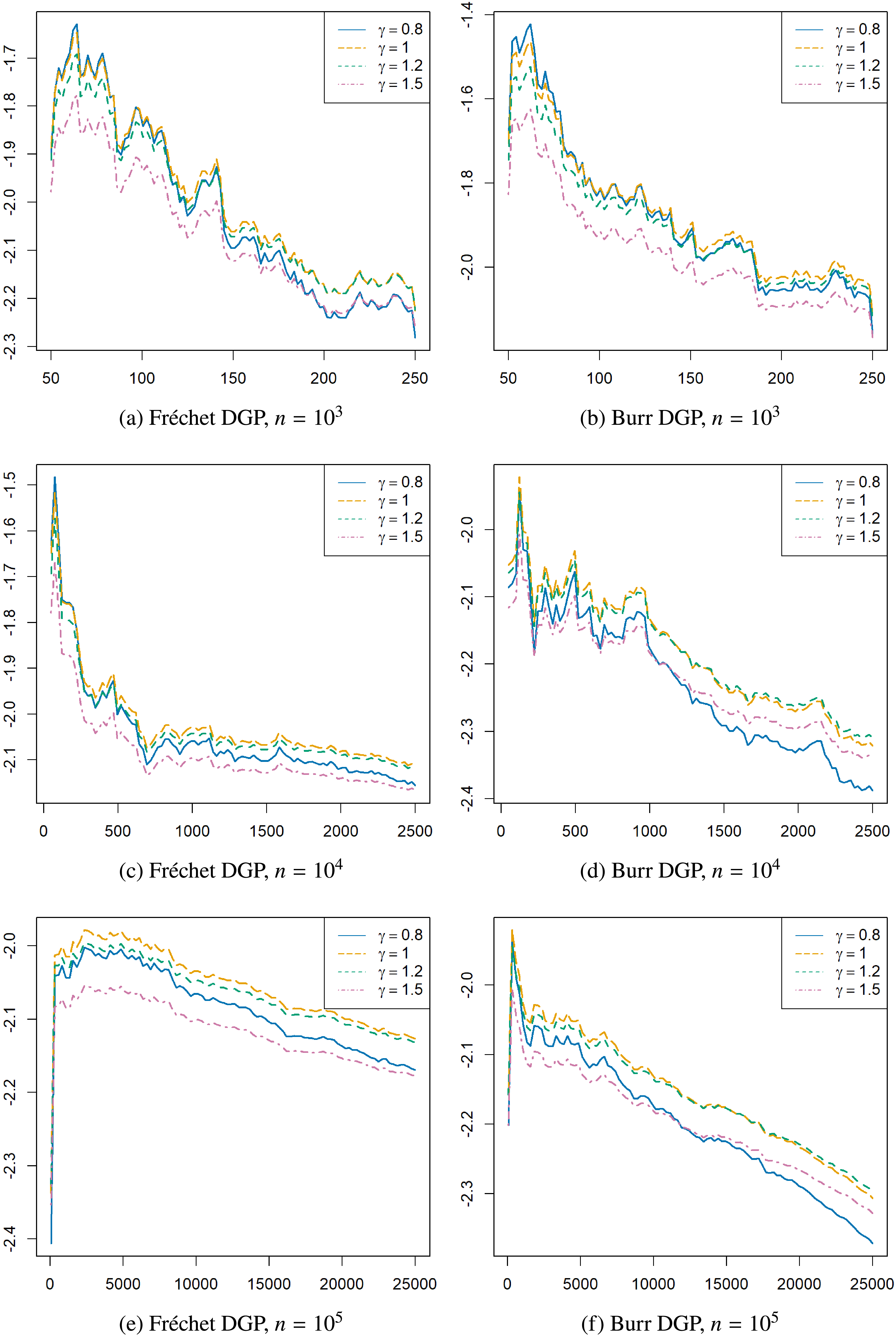
 γ∈{0.8,1,1.2,1.5}
 n=103,104,105
 γG=1
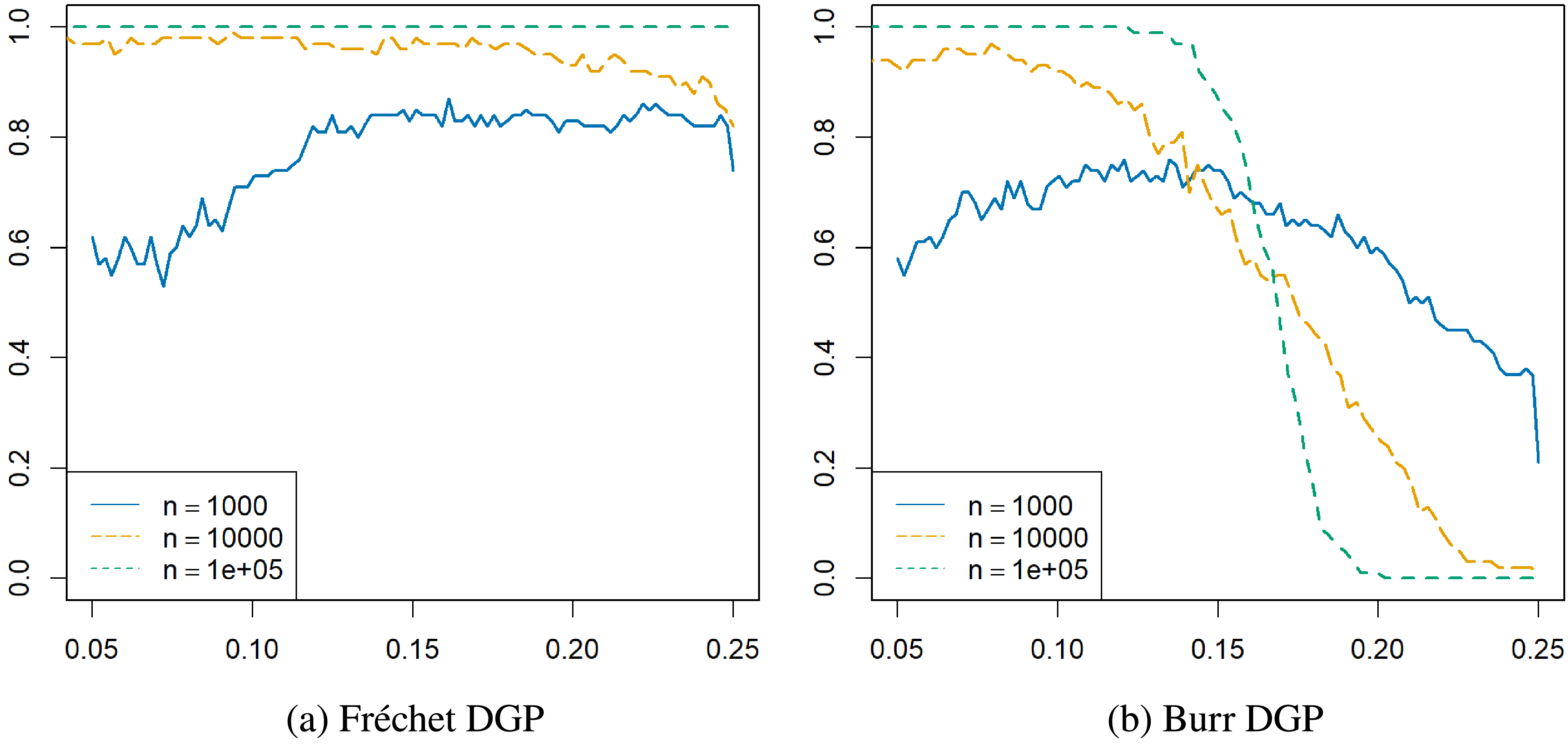
 γ=1
 γ∈{0.8,1,1.2,1.5}
 k/n
 n=103,104,105

 Yi=XiZi
 Zi
 γG=1
 γ∈{0.8,1,1.2,1.5}
 Xi1=1+i/n
 Xi2=1.5+0.5sin(6πi/n)
 n=103,104,105

 Yi=XiZi
 Zi
 γG=1
 γ∈{0.8,1,1.2,1.5}
 Xi1=1+i/n
 Xi2=1.5+0.5sin(6πi/n)
 n=103,104,105
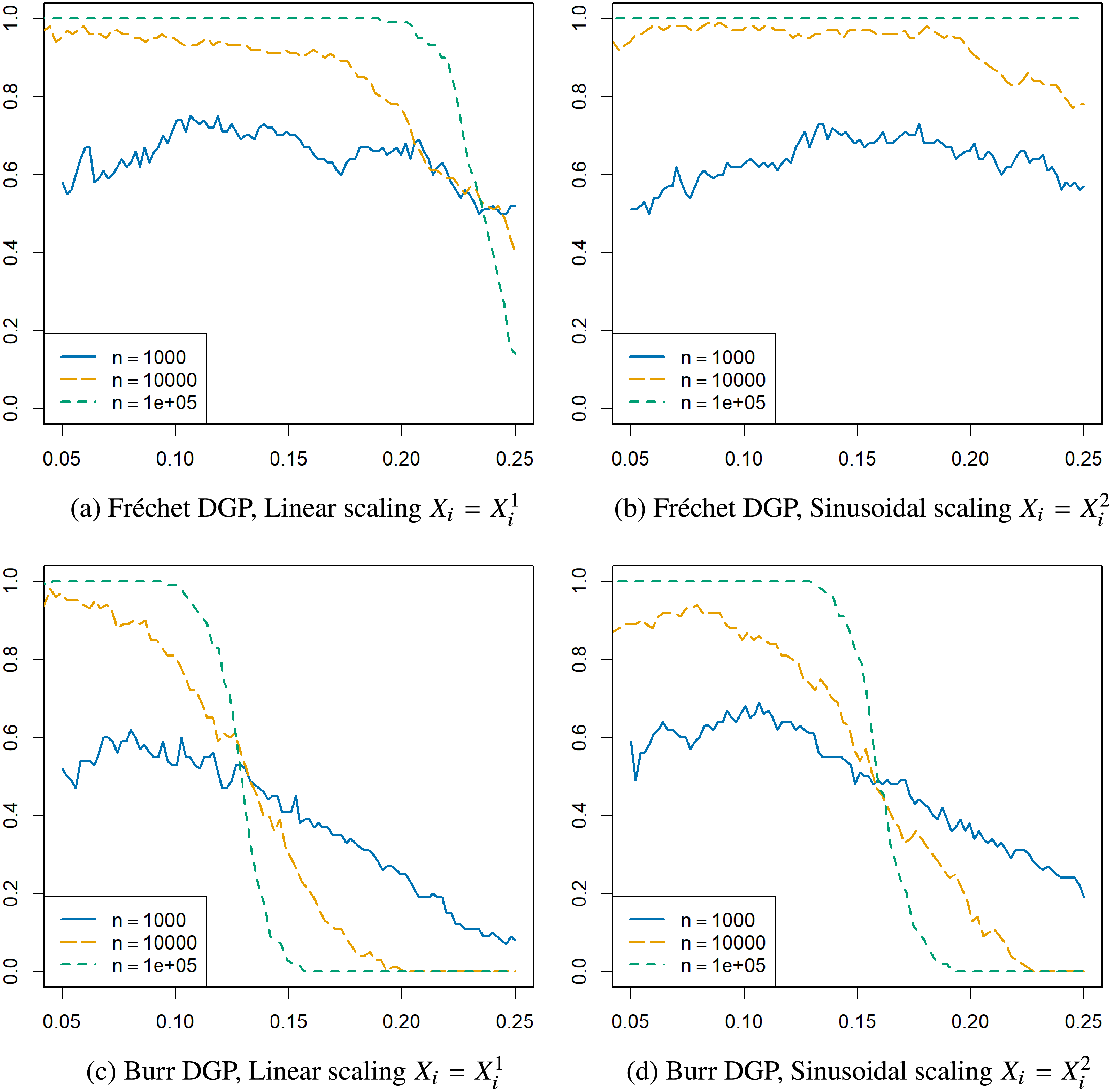
 γ=1
 γ∈{0.8,1,1.2,1.5}
 k/n
 n=103,104,105
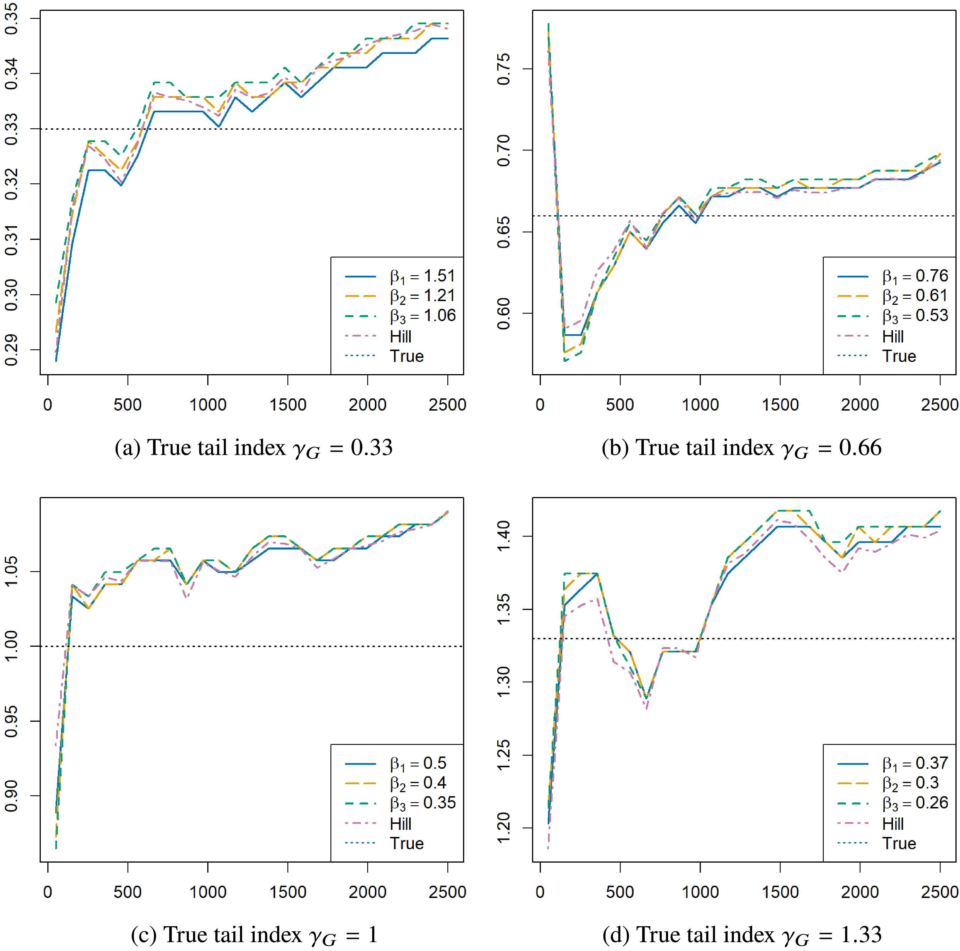
 γ^k
 n=104
 γG
 β1,β2,β3
 γG
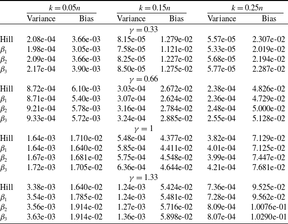
 β1,β2,
 β3
 n=104
 γ

 n=1,340
 γ∈{0.3,0.5,0.8,1,1.3}
 γ=1
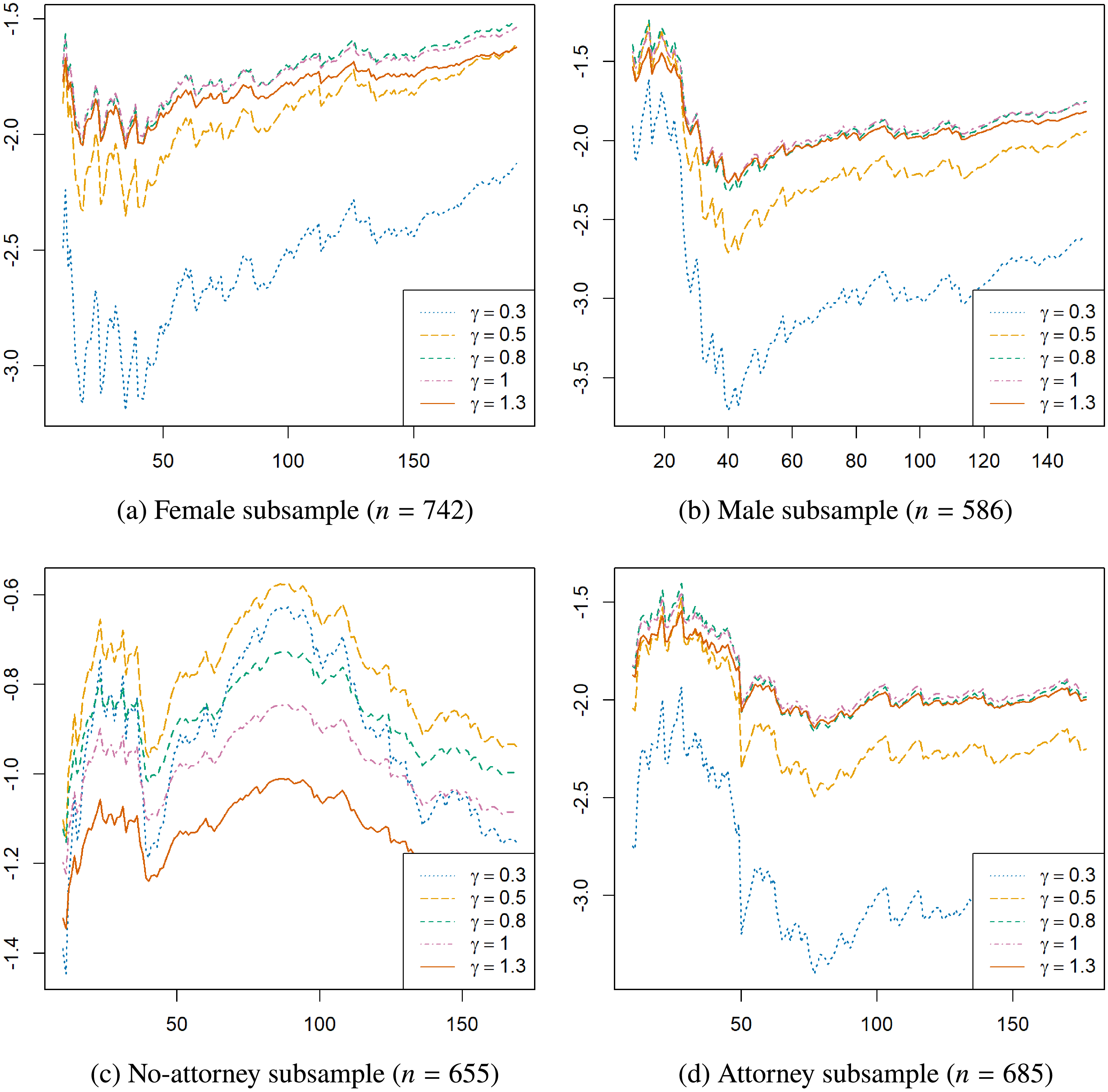

 Open access

