


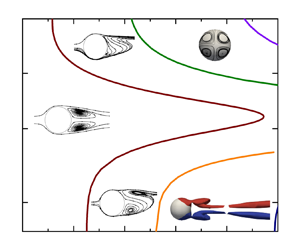



1. Introduction
With a constant external magnetic field, the Lorentz force as a non-contact method to control the movement of a solid particle has received special attention in metallurgy, such as producing immiscible alloys with a uniform distribution of solid particles in the matrix (Zheng et al. Reference Zheng, Zhong, Lei, Ren, Ren, Debray, Beaugnon and Fautrelle2015). It is noted that the path instability of a freely moving particle is closely related to its wake transition (Ern et al. Reference Ern, Risso, Fabre and Magnaudet2012). Therefore, comprehending the influence of a magnetic field on the wake transition around an obstacle can provide valuable insights for practical applications. Global linear stability analysis (LSA) has proven to be a valuable tool for determining the threshold of flow bifurcation past an obstacle at low Reynolds numbers. It aids in understanding the evolution of wake transition under different parameter settings. Hence, the present study focuses on the global LSA of flow past an insulated sphere under the influence of an external constant streamwise magnetic field.
Hydrodynamic flows past a fixed sphere without a magnetic field have been extensively investigated, which report two bifurcations at low Reynolds numbers. The first one is the regular bifurcation, at which the wake structure transitions from a steady axisymmetric wake to a steady plane symmetric wake. The second one is the Hopf bifurcation, at which the wake structure transitions from a steady plane symmetric wake to a periodic vortex shedding wake. These two transitions were illustrated to be supercritical by Thompson, Leweke & Provansal (Reference Thompson, Leweke and Provansal2001). Natarajan & Acrivos (Reference Natarajan and Acrivos1993) examined the stability of a steady axisymmetric base flow to three-dimensional perturbations with a global LSA, which found that the regular and Hopf bifurcations occurred at  $Re_c^I\approx 210$ and
 $Re_c^{II}\approx 277$, respectively. These two bifurcations resulted from the unstable stationary and oscillating modes with an azimuthal wavenumber
 $m=1$. Based on the same assumption of a steady axisymmetric base flow, Ghidersa & Dušek (Reference Ghidersa and Dušek2000) and Thompson et al. (Reference Thompson, Leweke and Provansal2001) considered the weakly nonlinear interaction between the stationary mode and the oscillating mode, a more accurate second critical Reynolds number was obtained,
 $Re_c^{II}\approx 272$ and 272.3, respectively. Furthermore, Citro et al. (Reference Citro, Siconolfi, Fabre, Giannetti and Luchini2017) performed a fully three-dimensional global stability analysis to accurately determine the second bifurcation at
 $Re_c^{II}=271.8$. In addition to the global stability analysis, the local stability analysis was also applied to the research of a flow past a sphere. To figure out the relation between global dynamics and their local instability characteristics, Pier (Reference Pier2008) examined the local absolute and convective properties of axisymmetric and planar symmetric basic flows under a parallel flow assumption, which established the existence of an absolutely unstable pocket.
When an external magnetic field is taken into consideration, the movement of a conducting fluid that deviates from parallel to the magnetic field generates electric currents, which in turn interact with the magnetic field, giving rise to the Lorentz force. This body force causes alterations in the flow configuration. In the case of flow around an obstacle, Yonas (Reference Yonas1967) did drag measurement experiments on a conducting flow past a sphere in the presence of a streamwise magnetic field. It was found that the magnetic field was able to completely damp dominant frequencies that existed in its corresponding hydrodynamic situation. Mutschke, Shatrov & Gerbeth (Reference Mutschke, Shatrov and Gerbeth1998) studied the flow past a cylinder and found that the critical Reynolds number, which was related to the flow transitioning from a steady state to an unsteady state, increased with an increase in the strength of the streamwise magnetic field. This indicates that the magnetic field is beneficial to stabilise the flow, which is possibly attributed to the Joule dissipation effect. The dampening effect of a constant magnetic field is generally acknowledged in various metallurgical applications (Chandrasekhar Reference Chandrasekhar2013).
Recent research has uncovered, however, some evidence indicating that the streamwise magnetic field not only exhibits its conventional damping effect but also plays a role in promoting flow instability. Mutschke et al. (Reference Mutschke, Gerbeth, Shatrov and Tomboulides2001) reported a non-monotonic behaviour of the temporal growth rate in a LSA of flow past a cylinder. They found that, under a strong magnetic field, the three-dimensional instability of the flow was amplified, resulting in a lower critical Reynolds number for the onset of a three-dimensional instability. Our previous direct numerical simulation (DNS) study on flow past a sphere confirmed a similar phenomenon (Pan, Zhang & Ni Reference Pan, Zhang and Ni2018). The wake transition from a steady axisymmetric flow to a steady plane symmetric flow was affected by the streamwise magnetic field, i.e. increasing the magnetic field resulted first in an increase then a decrease in the critical Reynolds number. Hence, it seems that a weak magnetic field will damp the growth of perturbation, while a strong magnetic field will promote its growth. Since the underlying mechanism behind this dual effect of the streamwise magnetic field remains unclear, a global LSA is employed to explore how the magnetic field damps or promotes the instability of flow past a sphere.
In the past few decades sensitivity analysis based on the adjoint method, as the extension of a LSA, has been developed and popularized to explore flow control dynamics (Chomaz Reference Chomaz2005; Camarri Reference Camarri2015). Experiments by Strykowski & Sreenivasan (Reference Strykowski and Sreenivasan1990) demonstrated that placing a small control cylinder in an appropriate position in the wake behind the main cylinder could suppress vortex shedding. To determine these locations in a more convenient theoretical approach, Giannetti & Luchini (Reference Giannetti and Luchini2007) regarded the action of the small cylinder as a local force acting in the perturbation momentum equation and defined a structural stability function. This function was introduced by investigating the greatest drift of the eigenvalue in a space under the influence of a modification in the structure, such as a small control cylinder force perturbation. It revealed the core region for the instability mechanism. Qualitative agreement was obtained between the theoretical prediction and the experimental data of Strykowski & Sreenivasan (Reference Strykowski and Sreenivasan1990). Marquet, Sipp & Jacquin (Reference Marquet, Sipp and Jacquin2008) argued that the small cylinder as a momentum force not only affected the perturbation equation but also the basic flow equation. They improved to model the small cylinder as a steady force acting on the basic flow and proposed the sensitivity function of the eigenvalue to this force. Their sensitivity analysis was applied to the global unstable mode that was responsible for the onset of vortex shedding. It determined the regions of the flow where a steady force acting on the base flow could stabilise the global unstable mode and suppress the vortex shedding. The regions of the control cylinder predicted by the sensitivity analysis in Marquet et al. (Reference Marquet, Sipp and Jacquin2008) compared well with the experimental results of Strykowski & Sreenivasan (Reference Strykowski and Sreenivasan1990). Furthermore, the sensitivity analysis was also applied to investigate the passive control of the secondary instability in the wake of a cylinder (Giannetti, Camarri & Citro Reference Giannetti, Camarri and Citro2019).
In recent years the sensitivity analysis method has been applied to explore the wake of a sphere by Meliga, Chomaz & Sipp (Reference Meliga, Chomaz and Sipp2009) and Citro et al. (Reference Citro, Siconolfi, Fabre, Giannetti and Luchini2017). The adjoint modes allowed them to determine the receptivity of each mode to particular initial conditions, external forcing or basic flow modifications. The core region of the instability mechanism was also localized in the same way by Giannetti & Luchini (Reference Giannetti and Luchini2007), where the eigenvalue was most sensitive to local modifications of the linearized Navier–Stokes operator. These sensitivity analyses provide valuable insights for defining control strategies in flow dynamics. Inspired by literature on sensitivity analyses, the magnetic field can be considered as a control factor, which will alter the stability properties of magnetohydrodynamic (MHD) flow. In fact, the Lorentz force acting on momentum equations alters the eigenvalue of the most unstable mode by modifying the base-flow configuration. Such sensitivity analyses to base-flow modifications and the Lorentz force are helpful to identify the core region where an increment of the magnetic field strength will produce the greatest drift of the global eigenvalue. Within this theoretical framework, the corresponding physical mechanism of the magnetic field's impact on flow instability can be explained. In this way, studying the influence of a magnetic field on the flow past a sphere turns into the problem that the sensitivity of the eigenvalue to base-flow modifications and the Lorentz force under different magnetic field intensities.
2. Problem formulation and validation
We consider an incompressible Newtonian fluid with electrical conductivity  $\sigma$, kinematic viscosity
 $\nu$ and density
 $\rho$ past an insulated sphere under a constant streamwise magnetic field
 ${\boldsymbol {B}}_0=B_0 {\boldsymbol {e}}_x$. The MHD governing equations are written based on a quasi-static approximation, in which the induced magnetic field can be negligible compared with the imposed magnetic field when the magnetic Reynolds number is much smaller than unity (Davidson Reference Davidson2001; Moreau Reference Moreau2013). Dimensionless flow variables, such as length, time, velocity, pressure, magnetic field, electrical potential and current are scaled with
 $d$,
 $d/U_\infty$,
 $U_\infty$,
 $\rho U_\infty ^2$,
 $B_0$,
 $d U_\infty B_0$ and
 $\sigma U_\infty B_0$, respectively. Here,
 $d$ and
 $U_\infty$ are the sphere diameter and uniform inflow velocity, respectively. Then non-dimensional MHD governing equations are governed by
 $$\begin{gather} \frac{\partial{{\boldsymbol{U}}}}{\partial t} + \boldsymbol{\nabla} {\boldsymbol{U}} \boldsymbol{\cdot} {\boldsymbol{U}} ={-}\boldsymbol{\nabla} P +\frac{1}{Re}\nabla^2 {\boldsymbol{U}} + N({\boldsymbol{J}} \times {\boldsymbol{e}}_x), \end{gather}$$
 $$\begin{gather}\boldsymbol{\nabla}\boldsymbol{\cdot} {\boldsymbol{U}} = 0, \end{gather}$$
 $$\begin{gather}\boldsymbol{\nabla}\boldsymbol{\cdot} {\boldsymbol{J}}=0, \end{gather}$$
where  $N({\boldsymbol {J}} \times {\boldsymbol {e}}_x)$ represents the Lorentz force acting on the conducting fluid by a magnetic field. Substituting Ohm's law
 ${\boldsymbol {J}}=-\boldsymbol {\nabla } \varPhi + {\boldsymbol {U}} \times {\boldsymbol {e}}_x$ into the equation of charge conservation (2.3), a Poisson equation for the electric potential can be derived as
 \begin{equation} \nabla^2 \varPhi-\boldsymbol{\nabla}\boldsymbol{\cdot} ({\boldsymbol{U}} \times {\boldsymbol{e}}_x)=0. \end{equation}
There are two important dimensionless parameters, the Reynolds number  ${Re}=U_\infty d / \nu$ and the interaction parameter
 ${N}=\sigma d B_0^2/\rho U_\infty$. They are measured by ratios of inertial to viscous forces and electromagnetic to inertial forces, respectively. The interaction parameter
 $N$ can be used to describe the strength of the electromagnetic field. Another dimensionless parameter is the Hartmann number
 ${Ha}=\sqrt {N Re}=d B_0 \sqrt {\sigma / \rho \nu }$, which represents the ratio of electromagnetic to viscous forces.
A standard cylindrical coordinate system  $(r, \theta, x)$ with the origin at the centre of the sphere is used in this paper, where
 $r$,
 $\theta$ and
 $x$ denote the radial, azimuthal and streamwise directions, respectively. Since the LSA in this paper is developed for steady and axisymmetric base flows whose physical quantities are uniformly distributed along the azimuth, the solutions of the base flow, stability and sensitivity equations require discretization on the two-dimensional
 $(x, r)$ plane. Figure 1 shows the flow configuration. The inlet boundary
 $\varGamma _{in}$ with a uniform incoming flow is located at
 $x=-l_1$, while the outlet boundary with a stress-free condition is located at
 $x=l_2$. The boundary
 $\varGamma _{ax}$ representing the symmetric axis is located at
 $r=0$. The external boundary
 $\varGamma _{ext}$ with an inviscid condition, where the normal velocity and tangential vorticity components are taken to be zero, is located at
 $r=h$. The sphere surface
 $\varGamma _{sp}$ is set with a non-slip condition.
Schematic of flow configuration.

2.1. Base-flow equations
For a certain value of the interaction number, when the Reynolds number is less than the threshold of the first instability, the flow is in a steady, axisymmetric state (Pan et al. Reference Pan, Zhang and Ni2018). The present paper investigates the response of the steady axisymmetric base flow to a small perturbation. The solution  $[{\boldsymbol {U}}_0,P_0,\varPhi _0]$ of a steady axisymmetric basic flow satisfies the following governing equations:
 $$\begin{gather} \boldsymbol{\nabla} {\boldsymbol{U}}_0 \boldsymbol{\cdot} {\boldsymbol{U}}_0 ={-}\boldsymbol{\nabla} P_0 +\frac{1}{Re}\nabla^2 {\boldsymbol{U}}_0 + N(-\boldsymbol{\nabla} \varPhi_0 + {\boldsymbol{U}}_0 \times {\boldsymbol{e}}_x)\times {\boldsymbol{e}}_x, \end{gather}$$
 $$\begin{gather}\boldsymbol{\nabla}\boldsymbol{\cdot} {\boldsymbol{U}}_0 = 0, \end{gather}$$
 $$\begin{gather}\nabla^2 \varPhi_0 - \boldsymbol{\nabla}\boldsymbol{\cdot} ({\boldsymbol{U}}_0 \times {\boldsymbol{e}}_x) = 0. \end{gather}$$
The boundary conditions are set as follows:  ${\boldsymbol {U}}_0=(0,0,1)^{\rm T}$ on the inlet;
 ${\boldsymbol {U}}_0={\boldsymbol {0}}$ on the sphere surface;
 $-P_0 {\boldsymbol {n}}+Re^{-1} \boldsymbol {\nabla } {\boldsymbol {U}}_0 \boldsymbol {\cdot } {\boldsymbol {n}}={\boldsymbol {0}}$ on the outlet;
 $U_{0r}=\partial U_{0x}/\partial r=0$ on the symmetric axis and external boundary. The potential meets
 $\partial \varPhi _0/ \partial {n}=({\boldsymbol {U}}_0 \times {\boldsymbol {e}}_x) \boldsymbol {\cdot } {\boldsymbol {n}}$ at all boundaries (Mück et al. Reference Mück, Günther, Müller and Bühler2000). Since the basic flow is axisymmetric, the electrical potential
 $\varPhi _0$ in the governing equation is decoupled from other physical quantities. According to its Poisson equation and boundary conditions, its spatial gradient can be inferred to be zero. That is, the electric potential
 $\varPhi _0$ is a uniformly distributed constant in space, and there is no need to solve
 $\varPhi _0$. Now, the current lines enclose along the azimuthal direction, and only the electromotive force (the second term of Ohm's law) contributes to the magnitude of the current. In this way, the Lorentz force can be represented as
 $N({\boldsymbol {U}}_0 \times {\boldsymbol {e}}_x\times {\boldsymbol {e}}_x)$.
2.2. Linear global stability equations
In LSA the total flow field  $[{\boldsymbol {U}},P,\varPhi ]$ is represented as a superposition of a basic flow
 $[{\boldsymbol {U}}_0,P_0,\varPhi _0]$ and an infinitesimal unsteady perturbation
 $[{\boldsymbol {u}}^\prime,p^\prime,\phi ^\prime ]$. The governing equations for the small perturbations are derived by subtracting the governing equations of the base flow from those of the total flow and neglecting quadratic high-order terms. Thus, the governing equations for the perturbations can be written as
 $$\begin{gather} \frac{\partial {\boldsymbol{u}}^\prime}{\partial t} + \boldsymbol{\nabla} {\boldsymbol{u}}^\prime \boldsymbol{\cdot} {\boldsymbol{U}}_0 + \boldsymbol{\nabla} {\boldsymbol{U}}_0 \boldsymbol{\cdot} {\boldsymbol{u}}^\prime ={-}\boldsymbol{\nabla} p^\prime +\frac{1}{Re}\nabla^2 {\boldsymbol{u}}^\prime + N(-\boldsymbol{\nabla} \phi^\prime + {\boldsymbol{u}}^\prime \times {\boldsymbol{e}}_x)\times {\boldsymbol{e}}_x , \end{gather}$$
 $$\begin{gather}\boldsymbol{\nabla}\boldsymbol{\cdot} {\boldsymbol{u}}^\prime = 0, \end{gather}$$
 $$\begin{gather}\nabla^2 \phi^\prime - \boldsymbol{\nabla}\boldsymbol{\cdot} ({\boldsymbol{u}}^\prime \times {\boldsymbol{e}}_x) = 0. \end{gather}$$
Since the basic flow is steady and axisymmetric, the perturbation can be expressed in the form of independent time-azimuthal modes,
 \begin{equation} [{\boldsymbol{u}}^\prime,p^\prime,\phi^\prime](r,\theta,x,t)=[{\boldsymbol{u}}, p,\phi](x,r)\exp({{\rm i}m\theta+\lambda t}), \end{equation}
where  $[{\boldsymbol {u}},p,\phi ](x,r)$ is referred to as the direct global mode. Here
 $m$ is the azimuthal wavenumber, which means that the velocity of global mode has
 $m$ pairs of counter-rotating vortical streamwise structures (Ghidersa & Dušek Reference Ghidersa and Dušek2000);
 $\lambda =\lambda _r+{\rm i} \lambda _i$ is the complex eigenvalue, where
 $\lambda _r$ and
 $\lambda _i$ denote the growth rate and angular frequency, respectively. The flow is unstable if
 $\lambda _r>0$ and a bifurcation will occur. The global mode with the maximal growth rate will be identified as the leading mode, in which
 $\lambda _i=0$ or
 $\lambda _i\neq 0$ is denoted as a stationary mode or an oscillating mode, respectively. Each time-azimuthal mode is demonstrated to behave like a propagating wave, which has a specific spatial signature (Ghidersa & Dušek Reference Ghidersa and Dušek2000). By substituting (2.11) into (2.8)–(2.10), the generalized eigenvalue equations for a time-azimuthal mode can be formulated as
 \begin{align} &\lambda u_r + U_{0r}\frac{\partial u_r}{\partial r} + U_{0x}\frac{\partial u_r}{\partial x} + u_r\frac{\partial U_{0r}}{\partial r} + u_x\frac{\partial U_{0r}}{\partial x} \nonumber\\ &\quad ={-} \frac{\partial p}{\partial r} + \frac{1}{Re}\left(\frac{\partial^2 u_r}{\partial r^2} + \frac{\partial^2 u_r}{\partial x^2} + \frac{1}{r} \frac{\partial u_r}{\partial r} - \frac{u_r}{r^2} - m^2\frac{u_r}{r^2} - {\rm i}2m\frac{u_\theta}{r^2}\right) - N\left({\rm i}m\frac{\phi}{r} + u_r\right), \end{align}
 \begin{align} &\lambda u_{\theta} + U_{0r}\frac{\partial u_{\theta}}{\partial r} + U_{0x}\frac{\partial u_{\theta}}{\partial x} + \frac{U_{0r} u_{\theta}}{r} \nonumber\\ &\quad ={-} {\rm i}m \frac{p}{r} + \frac{1}{Re}\left(\frac{\partial^2 u_{\theta}}{\partial r^2} + \frac{\partial^2 u_{\theta}}{\partial x^2} + \frac{1}{r} \frac{\partial u_{\theta}}{\partial r} - \frac{u_{\theta}}{r^2} - m^2\frac{u_{\theta}}{r^2} + {\rm i}2m\frac{u_r}{r^2}\right) + N\left(\frac{\partial \phi}{\partial r} - u_{\theta}\right), \end{align}
 \begin{gather} \lambda u_x + U_{0r}\frac{\partial u_x}{\partial r} + U_{0x}\frac{\partial u_x}{\partial x} + u_r\frac{\partial U_{0x}}{\partial r} + u_x\frac{\partial U_{0x}}{\partial x} \nonumber\\ \hskip7pc ={-} \frac{\partial p}{\partial x} + \frac{1}{Re}\left(\frac{\partial^2 u_x}{\partial r^2} + \frac{\partial^2 u_x}{\partial x^2} + \frac{1}{r} \frac{\partial u_x}{\partial r} - m^2\frac{u_x}{r^2}\right), \end{gather}
 \begin{gather} \frac{\partial u_r}{\partial r} + \frac{\partial u_x}{\partial x} + \frac{u_r}{r} + {\rm i}m \frac{u_{\theta}}{r}= 0 , \end{gather}
 \begin{gather} \frac{1}{r} \frac{\partial \phi}{\partial r} + \frac{\partial^2 \phi}{\partial r^2} - m^2\frac{\phi}{r^2} + \frac{\partial^2 \phi}{\partial x^2} + {\rm i}m \frac{u_r}{r} - \frac{\partial u_{\theta}}{\partial r} - \frac{u_{\theta}}{r} = 0 . \end{gather}
It is important to note that the  $\boldsymbol {\nabla }$ operator consists of the algebraic operations (
 $i*m$ multiplications) and differential operations (
 $x$ and
 $r$ derivatives). The boundary conditions are set as follows:
 ${\boldsymbol {u}}={\boldsymbol {0}}$ on the inlet and sphere surface;
 $-p {\boldsymbol {n}}+Re^{-1} \boldsymbol {\nabla } {\boldsymbol {u}} \boldsymbol {\cdot } {\boldsymbol {n}}={\boldsymbol {0}}$ on the outlet;
 $u_r=\partial u_\theta / \partial r=\partial u_x / \partial r=0$ on the external boundary;
 $u_r=\partial u_x/\partial r=\partial p/\partial r=0$ if
 $m=0$,
 $\partial u_r/\partial r=\partial u_\theta /\partial r=u_x=p=0$ if
 $|m|=1$,
 $u_r=u_\theta =u_x=p=0$ if
 $|m|\geq 2$ on the symmetric axis (Tchoufag, Magnaudet & Fabre Reference Tchoufag, Magnaudet and Fabre2013);
 $\partial \phi / \partial n=({\boldsymbol {u}} \times {\boldsymbol {e}}_x) \boldsymbol {\cdot } {\boldsymbol {n}}$ on all the boundaries. For each azimuthal wavenumber
 $m$, if
 $\lambda$ and
 $[{\boldsymbol {u}},p,\phi ]$ are the solutions of the eigenvalue equations, their conjugated counterparts
 $\lambda ^*$ and
 $[{\boldsymbol {u}}^*,p^*,\phi ^*]$ are the solutions of the eigenvalue equations for
 $-m$. It is noted that the following governing equations are given in a vector form for concision.
2.3. Sensitivity equations
The sensitivity analysis is considered here to investigate the variation of a given eigenvalue  $\lambda$ resulted from the base-flow modifications and the Lorentz force variations. These two sensitivity analyses discuss the flow instability from different perspectives. There is a close relationship between them, since the base-flow modifications are induced by the Lorentz force. These two sensitivity functions are defined as the gradient of the eigenvalue with respect to the base flow
 $[\boldsymbol {\nabla }_{{\boldsymbol {U}}_0} \lambda, \boldsymbol {\nabla }_{P_0} \lambda, \boldsymbol {\nabla }_{\varPhi _0} \lambda ]$ and the Lorentz force
 $\boldsymbol {\nabla }_{{\boldsymbol {F}}} \lambda$, respectively. Their expressions are derived by a general theoretical formation introduced by Marquet et al. (Reference Marquet, Sipp and Jacquin2008) and Giannetti, Camarri & Luchini (Reference Giannetti, Camarri and Luchini2010). When considering small variations of the Lorentz force
 $\delta {\boldsymbol {F}}$, base-flow modifications
 $[\delta {\boldsymbol {U}}_0, \delta P_0, \delta \varPhi _0]$ will be induced through (2.5)–(2.7). As a consequence, the variations of eigenvalue
 $\delta \lambda$ and eigenmode
 $[\delta {\boldsymbol {u}}, \delta p, \delta \phi ]$ are also induced as they are solutions of the eigenvalue problem given by (2.8)–(2.10), which is associated with the base flow. Firstly, the variations of base flow
 $[\delta {\boldsymbol {U}}_0, \delta P_0, \delta \varPhi _0]$ are governed by the following equations:
 $$\begin{gather} A(\delta {\boldsymbol{U}}_0,{\boldsymbol{U}}_0) ={-}\boldsymbol{\nabla} \delta P_0 +\frac{1}{Re}\nabla^2 \delta {\boldsymbol{U}}_0 + N(-\boldsymbol{\nabla} \delta \varPhi_0 + \delta {\boldsymbol{U}}_0 \times {\boldsymbol{e}}_x) \times {\boldsymbol{e}}_x + \delta {\boldsymbol{F}} , \end{gather}$$
 $$\begin{gather}\boldsymbol{\nabla}\boldsymbol{\cdot}\delta {\boldsymbol{U}}_0 = 0 , \end{gather}$$
 $$\begin{gather}\nabla^2 \delta \varPhi_0 - \boldsymbol{\nabla}\boldsymbol{\cdot}(\delta {\boldsymbol{U}}_0\times {\boldsymbol{e}}_x) = 0 . \end{gather}$$
Here, the advection term  $\boldsymbol {\nabla } {\boldsymbol {U}}_0 \boldsymbol {\cdot }\delta {\boldsymbol {U}}_0 + \boldsymbol {\nabla } \delta {\boldsymbol {U}}_0 \boldsymbol {\cdot } {\boldsymbol {U}}_0$ is denoted as
 $A(\delta {\boldsymbol {U}}_0,{\boldsymbol {U}}_0)$ for convenience. The variation of Lorentz force
 $\delta {\boldsymbol {F}}$ is assumed to be small enough to produce small variations of the base flow and the global mode. So a linearized analysis can be carried out. The variations of the global mode are governed by
 $$\begin{gather} \delta \lambda {\boldsymbol{u}}+\lambda \delta {\boldsymbol{u}}+ A(\delta {\boldsymbol{U}}_0,{\boldsymbol{u}}) + A({\boldsymbol{U}}_0,\delta {\boldsymbol{u}}) ={-} \boldsymbol{\nabla} \delta p + \frac{1}{Re} \nabla^2 \delta {\boldsymbol{u}} + N(-\boldsymbol{\nabla} \delta \phi+ \delta {\boldsymbol{u}} \times {\boldsymbol{e}}_x) \times {\boldsymbol{e}}_x, \end{gather}$$
 $$\begin{gather}\boldsymbol{\nabla}\boldsymbol{\cdot} \delta {\boldsymbol{u}} = 0, \end{gather}$$
 $$\begin{gather}\nabla^2 \delta \phi - \boldsymbol{\nabla}\boldsymbol{\cdot} (\delta {\boldsymbol{u}} \times {\boldsymbol{e}}_x)=0 . \end{gather}$$
Then, the complex Lagrange multipliers  $[{\boldsymbol {U}}_0^{\dagger}, P_0^{\dagger}, \varPhi _0^{\dagger} ]$ and
 $[{\boldsymbol {u}}^{\dagger}, p^{\dagger}, \phi ^{\dagger} ]$, referred to as the complex adjoint base flow and the complex adjoint global mode, are introduced to obtain a generalized Lagrange identity. The Lagrange identity is constructed as
 \begin{align}
&\langle {\boldsymbol{U}}_0^{\dagger},
\text{(2.17)} \rangle + \langle P_0^{\dagger},
\text{(2.18)} \rangle + \langle
\varPhi_0^{\dagger}, \text{(2.19)} \rangle +
\langle {\boldsymbol{u}}^{\dagger},
\text{(2.20)} \rangle + \langle
p^{\dagger}, \text{(2.21)} \rangle\nonumber\\
&\quad + \langle \phi^{\dagger}, \text{(2.22)}
\rangle =0 ,
\end{align}
where the operation symbol  $\langle,\rangle$ is the inner product on the whole domain
 $\varOmega$ defined by
 $\langle {\boldsymbol {a}}, {\boldsymbol {b}} \rangle =\int _\varOmega {\boldsymbol {a}}^\ast \boldsymbol {\cdot } {\boldsymbol {b}} \,{\rm d} \varOmega$. Placing the terms related to
 $[\delta {\boldsymbol {U}}_0, \delta P_0, \delta \varPhi _0]$ and
 $[\delta {\boldsymbol {u}},\delta p, \delta \phi ]$ on the right-hand side of the equation, the Lagrange identity turns into (2.24) as
 \begin{align} &\int_{\varOmega} \delta{\boldsymbol{F}} \boldsymbol{\cdot} {\boldsymbol{U}}_0^{{\dagger} \ast} - \delta\lambda{\boldsymbol{u}} \boldsymbol{\cdot} {\boldsymbol{u}}^{{\dagger} \ast} \,{\rm d} \varOmega \nonumber\\ &\quad = \int_{\varOmega} \left[ \left(A(\delta {\boldsymbol{U}}_0,{\boldsymbol{U}}_0) +\boldsymbol{\nabla} \delta P_0 -\frac{1}{Re}\nabla^2 \delta {\boldsymbol{U}}_0 + N(\boldsymbol{\nabla} \delta \varPhi_0 - \delta {\boldsymbol{U}}_0 \times {\boldsymbol{e}}_x) \times {\boldsymbol{e}}_x\right) \boldsymbol{\cdot} {\boldsymbol{U}}_0^{{\dagger} \ast}\right. \nonumber\\ &\qquad \left. + (\boldsymbol{\nabla}\boldsymbol{\cdot} \delta {\boldsymbol{U}}_0) P_0^{{\dagger} \ast} + (\nabla^2 \delta \varPhi_0 - \boldsymbol{\nabla} \boldsymbol{\cdot} (\delta {\boldsymbol{U}}_0\times {\boldsymbol{e}}_x)) \varPhi_0^{{\dagger} \ast} \vphantom{\left(A(\delta {\boldsymbol{U}}_0,{\boldsymbol{U}}_0) +\boldsymbol{\nabla} \delta P_0 -\frac{1}{Re}\nabla^2 \delta {\boldsymbol{U}}_0 + N(\boldsymbol{\nabla} \delta \varPhi_0 - \delta {\boldsymbol{U}}_0 \times {\boldsymbol{e}}_x) \times {\boldsymbol{e}}_x\right)} \right] {\rm d} \varOmega \nonumber\\ &\qquad + \int_{\varOmega} \left[ \left(\vphantom{\left(A(\delta {\boldsymbol{U}}_0,{\boldsymbol{U}}_0) +\boldsymbol{\nabla} \delta P_0 -\frac{1}{Re}\nabla^2 \delta {\boldsymbol{U}}_0 + N(\boldsymbol{\nabla} \delta \varPhi_0 - \delta {\boldsymbol{U}}_0 \times {\boldsymbol{e}}_x) \times {\boldsymbol{e}}_x\right)}\lambda \delta {\boldsymbol{u}} + A(\delta {\boldsymbol{U}}_0,{\boldsymbol{u}}) + A({\boldsymbol{U}}_0,\delta {\boldsymbol{u}}) +\boldsymbol{\nabla} \delta p \right.\right.\nonumber\\ &\qquad \left.-\frac{1}{Re}\nabla^2 \delta {\boldsymbol{u}} + N(\boldsymbol{\nabla} \delta \phi-\delta {\boldsymbol{u}} \times {\boldsymbol{e}}_x)\times {\boldsymbol{e}}_x \right) \boldsymbol{\cdot} {\boldsymbol{u}}^{{\dagger} \ast} \nonumber\\ &\qquad \left. + (\boldsymbol{\nabla}\boldsymbol{\cdot}\delta {\boldsymbol{u}}) p^{{\dagger} \ast} + (\nabla^2 \delta \phi - \boldsymbol{\nabla}\boldsymbol{\cdot}(\delta {\boldsymbol{u}}\times {\boldsymbol{e}}_x)) \phi^{{\dagger} \ast} \vphantom{\left(A(\delta {\boldsymbol{U}}_0,{\boldsymbol{U}}_0) +\boldsymbol{\nabla} \delta P_0 -\frac{1}{Re}\nabla^2 \delta {\boldsymbol{U}}_0 + N(\boldsymbol{\nabla} \delta \varPhi_0 - \delta {\boldsymbol{U}}_0 \times {\boldsymbol{e}}_x) \times {\boldsymbol{e}}_x\right)}\right] {\rm d}\varOmega, \end{align}
 \begin{align} &\int_{\varOmega}
\delta{\boldsymbol{F}} \boldsymbol{\cdot}
{\boldsymbol{U}}_0^{{\dagger} \ast} -
\delta\lambda{\boldsymbol{u}} \boldsymbol{\cdot}
{\boldsymbol{u}}^{{\dagger}\ast} \,{\rm d} \varOmega \nonumber\\
&\quad = \int_{\varOmega}
\left[\left(\vphantom{-\frac{1}{Re}}
A^{\dagger}({\boldsymbol{U}}_0^{\dagger},{\boldsymbol{U}}_0) +
A^{\dagger}({\boldsymbol{u}}^{\dagger},{\boldsymbol{u}}^\ast) +
\boldsymbol{\nabla} P_0^{\dagger}\right.\right.\nonumber\\
&\qquad \left. -\,\frac{1}{Re}\nabla^2
{\boldsymbol{U}}_0^{\dagger} + N( \nabla \varPhi_0^{\dagger}-
{\boldsymbol{U}}_0^{\dagger} \times {\boldsymbol{e}}_x)\times
{\boldsymbol{e}}_x\right)^\ast \boldsymbol{\cdot} \delta
{\boldsymbol{U}}_0 \nonumber\\ &\qquad \left. +\,
(\boldsymbol{\nabla} \boldsymbol{\cdot}
{\boldsymbol{U}}_0^{\dagger})^\ast \delta P_0
+ (\nabla^2 \varPhi_0^{\dagger} - \boldsymbol{\nabla}
\boldsymbol{\cdot}({\boldsymbol{U}}_0^{\dagger}\times
{\boldsymbol{e}}_x))^\ast \delta
\varPhi_0 \vphantom{\frac{1}{Re}}\right]{\rm d}
\varOmega\nonumber\\ &\qquad + \int_{\varOmega}
\left[\left(\lambda^\ast {\boldsymbol{u}}^{\dagger} +
A^{\dagger}({\boldsymbol{u}}^{\dagger},{\boldsymbol{U}}_0)
+\boldsymbol{\nabla} p^{\dagger} -\frac{1}{Re}\nabla^2
{\boldsymbol{u}}^{\dagger} +N(\boldsymbol{\nabla} \phi^{\dagger} -
{\boldsymbol{u}}^{\dagger} \times {\boldsymbol{e}}_x)\times
{\boldsymbol{e}}_x \right)^\ast \boldsymbol{\cdot} \delta
{\boldsymbol{u}} \right.\nonumber\\ &\qquad\left. +\,
(\boldsymbol{\nabla}\boldsymbol{\cdot}{\boldsymbol{u}}^{\dagger})^\ast
\delta p + (\nabla^2 \phi^{\dagger} -
\boldsymbol{\nabla}\boldsymbol{\cdot}
({\boldsymbol{u}}^{\dagger}\times {\boldsymbol{e}}_x))^\ast
\delta \phi \vphantom{\frac{1}{Re}}\right] {\rm d}\varOmega
\nonumber\\ &\qquad + \oint_{\partial \varOmega}
\left(({\boldsymbol{u}}^\ast \boldsymbol{\cdot}
{\boldsymbol{n}}) {\boldsymbol{u}}^{\dagger} +
({\boldsymbol{U}}_0 \boldsymbol{\cdot}
{\boldsymbol{n}}){\boldsymbol{U}}_0^{\dagger} - N \varPhi_0^{\dagger}
{\boldsymbol{n}} \times {\boldsymbol{e}}_x -
{\boldsymbol{n}} P_0^{\dagger} + \frac{1}{Re}
(\boldsymbol{\nabla} {\boldsymbol{U}}_0^{\dagger})
\boldsymbol{\cdot} {\boldsymbol{n}} \right)^\ast
\boldsymbol{\cdot} \delta {\boldsymbol{U}}_0 \,{\rm d}s
\nonumber\\ &\qquad - \oint_{\partial \varOmega}
{\boldsymbol{n}} \boldsymbol{\cdot} ( \nabla \varPhi_0^{\dagger}
- {\boldsymbol{U}}_0^{\dagger} \times {\boldsymbol{e}}_x )^\ast
\delta \varPhi_0 \,{\rm d}s \nonumber\\ &\qquad +
\oint_{\partial \varOmega} \left(({\boldsymbol{U}}_0
\boldsymbol{\cdot} {\boldsymbol{n}}){\boldsymbol{u}}^{\dagger} -
N \phi^{\dagger} {\boldsymbol{n}} \times {\boldsymbol{e}}_x -
{\boldsymbol{n}} p^{\dagger} + \frac{1}{Re} (\boldsymbol{\nabla}
{\boldsymbol{u}}^{\dagger})\boldsymbol{\cdot}
{\boldsymbol{n}}\right)^\ast \boldsymbol{\cdot} \delta
{\boldsymbol{u}} \,{\rm d}s \nonumber\\ &\qquad -
\oint_{\partial \varOmega} {\boldsymbol{n}}
\boldsymbol{\cdot} (\boldsymbol{\nabla} \phi^{\dagger} -
{\boldsymbol{u}}^{\dagger} \times {\boldsymbol{e}}_x )^\ast
\delta \phi \,{\rm d}s .
\end{align}
In order to shift the action of the differential operators  $\boldsymbol {\nabla }$ in (2.24) from the direct fields to the adjoint fields, integration by parts and the divergence theorem are used. As a result, a new form of the identity containing boundary integral terms, which is equivalent to (2.24), is obtained in (2.25).
Here, the advection term of adjoint field  $\boldsymbol {\nabla } {\boldsymbol {b}}^{T} \boldsymbol {\cdot } {\boldsymbol {a}} -\boldsymbol {\nabla } {\boldsymbol {a}} {\cdot } {\boldsymbol {b}}$ is denoted as
 $A^{\dagger} ({\boldsymbol {a}},{\boldsymbol {b}})$ to simplify the expression. Eliminating the first two rows on the right-hand side of (2.25) leads to the definition of the adjoint base-flow equations
 $$\begin{gather} A^{\dagger}({\boldsymbol{U}}_0^{\dagger},{\boldsymbol{U}}_0) + \boldsymbol{\nabla} P_0^{\dagger} -\frac{1}{Re}\nabla^2 {\boldsymbol{U}}_0^{\dagger} + N(\boldsymbol{\nabla} \varPhi_0^{\dagger}- {\boldsymbol{U}}_0^{\dagger} \times {\boldsymbol{e}}_x) \times {\boldsymbol{e}}_x ={-}A^{\dagger}({\boldsymbol{u}}^{\dagger},{\boldsymbol{u}}^\ast) , \end{gather}$$
 $$\begin{gather}\boldsymbol{\nabla}\boldsymbol{\cdot} {\boldsymbol{U}}_0^{\dagger} = 0 , \end{gather}$$
 $$\begin{gather}\nabla^2 \varPhi_0^{\dagger} - \boldsymbol{\nabla}\boldsymbol{\cdot} ({\boldsymbol{U}}_0^{\dagger}\times {\boldsymbol{e}}_x)=0. \end{gather}$$
For the same reason stated in § 2.1, the electric potential of the adjoint base flow also does not need to be solved. By eliminating the boundary terms on the sixth and seventh right-hand rows of (2.25), the following boundary conditions for the adjoint base flow are obtained:  ${\boldsymbol {U}}_0^{\dagger} ={\boldsymbol {0}}$ at the inlet and on the sphere surface;
 $\partial U_{0x}^{\dagger} / \partial r= U_{0r} = 0$ at the external boundary and symmetric axis;
 $-P_0^{\dagger} {\boldsymbol {n}} + Re^{-1} (\boldsymbol {\nabla } {\boldsymbol {U}}_0^{\dagger} ) \boldsymbol {\cdot } {\boldsymbol {n}}= -({\boldsymbol {u}}^\ast \boldsymbol {\cdot } {\boldsymbol {n}}) {\boldsymbol {u}}^{\dagger} - ({\boldsymbol {U}}_0 \boldsymbol {\cdot } {\boldsymbol {n}}){\boldsymbol {U}}_0^{\dagger} + N \varPhi _0^{\dagger} {\boldsymbol {n}} \times {\boldsymbol {e}}_x$ at the outlet.
Analogously, by eliminating the third and fourth rows on the right-hand side of (2.25), equations associated to the adjoint global mode  $[{\boldsymbol {u}}^{\dagger}, p^{\dagger}, \phi ^{\dagger} ]$ can be obtained as
 $$\begin{gather} \lambda^\ast {\boldsymbol{u}}^{\dagger} + A^{\dagger}({\boldsymbol{u}}^{\dagger},{\boldsymbol{U}}_0) +\boldsymbol{\nabla} p^{\dagger} -\frac{1}{Re}\nabla^2 {\boldsymbol{u}}^{\dagger} + N(\boldsymbol{\nabla} \phi^{\dagger} - {\boldsymbol{u}}^{\dagger} \times {\boldsymbol{e}}_x) \times {\boldsymbol{e}}_x = 0 , \end{gather}$$
 $$\begin{gather}\boldsymbol{\nabla}\boldsymbol{\cdot} {\boldsymbol{u}}^{\dagger} = 0 , \end{gather}$$
 $$\begin{gather}\nabla^2 \phi^{\dagger} - \boldsymbol{\nabla}\boldsymbol{\cdot} ({\boldsymbol{u}}^{\dagger}\times {\boldsymbol{e}}_x)=0. \end{gather}$$
By eliminating the last two rows on the right-hand side of (2.25), the following boundary conditions for the adjoint global mode can be obtained:  ${\boldsymbol {u}}^{\dagger} ={\boldsymbol {0}}$ at the inlet and on the sphere surface;
 $\partial u_x^{\dagger} / \partial r= u_r^{\dagger} = 0$ at the external boundary;
 $-p^{\dagger} {\boldsymbol {n}} + Re^{-1} (\nabla {\boldsymbol {u}}^{\dagger} ) \boldsymbol {\cdot } {\boldsymbol {n}} = -({\boldsymbol {U}}_0 \boldsymbol {\cdot } {\boldsymbol {n}}) {\boldsymbol {u}}^{\dagger} + N \phi ^{\dagger} {\boldsymbol {n}} \times {\boldsymbol {e}}_x$ at the outlet;
 $u^{\dagger} _r=\partial u^{\dagger} _x/\partial r=\partial p^{\dagger} /\partial r=0$ if
 $m=0$,
 $\partial u^{\dagger} _r/\partial r=\partial u^{\dagger} _\theta /\partial r=u^{\dagger} _x=p^{\dagger} =0$ if
 $|m|=1$,
 $u^{\dagger} _r=u^{\dagger} _\theta =u^{\dagger} _x=p^{\dagger} =0$ if
 $|m|\geq 2$ at the symmetric axis,
 $\partial \phi ^{\dagger} / \partial n=({\boldsymbol {u}}^{\dagger} \times {\boldsymbol {e}}_x)\boldsymbol {\cdot } {\boldsymbol {n}}$ on all the boundaries.
Comparing the governing equations of the direct global mode (2.8)–(2.10) and the adjoint global mode (2.29)–(2.31), it is noted that the difference comes from the advection operator. Here  $\boldsymbol {\nabla }{\boldsymbol {u}} \boldsymbol {\cdot } {\boldsymbol {U}}_0$ indicates the downstream transport of the direct global mode by the base flow, while
 $-\boldsymbol {\nabla }{\boldsymbol {u}}^{\dagger} \boldsymbol {\cdot } {\boldsymbol {U}}_0$ indicates the upstream transport of the adjoint global mode by the base flow. Such a difference results in the spatial separation of the direct mode and adjoint mode in the streamwise direction. The items of
 $\boldsymbol {\nabla }{\boldsymbol {U}}_0 \boldsymbol {\cdot } {\boldsymbol {u}}$ and
 $\boldsymbol {\nabla }{\boldsymbol {U}}_0^T \boldsymbol {\cdot } {\boldsymbol {u}}^{\dagger}$ correspond to the production of the direct mode and adjoint mode, respectively. Marquet et al. (Reference Marquet, Lombardi, Chomaz, Sipp and Jacquin2009) pointed out that the direct mode and the adjoint mode tended to be mutually orthogonal owing to the transpose of the base-flow velocity gradient. Meliga et al. (Reference Meliga, Chomaz and Sipp2009) explained the orthogonality of direct and adjoint modes from the energy point of view. They reported that the perturbation energy of the direct mode was mainly composed of streamwise velocity, while the adjoint mode was mainly composed of the cross-stream velocity.
After obtaining the adjoint base-flow equations and the adjoint global mode equations, coupling with their corresponding boundary conditions, the Lagrange identity (2.25) finally becomes  $\langle {\boldsymbol {U}}^{\dagger} _0,\delta {\boldsymbol {F}} \rangle = \delta \lambda \langle {\boldsymbol {u}}^{\dagger},{\boldsymbol {u}} \rangle$. Hence, the eigenvalue variation
 $\delta \lambda$ due to the change of Lorentz force
 $\delta {\boldsymbol {F}}$ can be obtained from
 \begin{equation} \delta\lambda=\frac{\langle {\boldsymbol{U}}^{\dagger}_0,\delta {\boldsymbol{F}} \rangle}{\langle {\boldsymbol{u}}^{\dagger},{\boldsymbol{u}} \rangle} . \end{equation}
Here,  $\langle {\boldsymbol {u}}^{\dagger},{\boldsymbol {u}} \rangle$ is a normalization condition for the adjoint global mode and it can be simply seen as equaling to unity. Hence, there is
 $\delta \lambda =\langle {\boldsymbol {U}}^{\dagger} _0,\delta {\boldsymbol {F}} \rangle$. According to the physical definition of the sensitivity function of the eigenvalue to Lorentz force, it establishes the connection between the small variation of the Lorentz force and the small drift of the eigenvalue, which can be expressed as
 $\delta \lambda =\langle \boldsymbol {\nabla }_{{\boldsymbol {F}}} \lambda, \delta {\boldsymbol {F}} \rangle$. A so-called sensitivity function of a selected eigenvalue to Lorentz force
 $\boldsymbol {\nabla }_{{\boldsymbol {F}}} \lambda$ is obtained by knowledge of the adjoint base-flow field
 ${\boldsymbol {U}}_0^{{\dagger} }$ as
 \begin{equation} \boldsymbol{\nabla}_{\boldsymbol{F}} \lambda={\boldsymbol{U}}_0^{{\dagger}}. \end{equation}
The sensitivity function to Lorentz force determines the core region of the flow, where the eigenvalue  $\lambda$ is most sensitive to the variations of Lorentz force. The effect of the Lorentz force in this region is therefore crucial in determining the global eigenvalue. Such a concept is an extension to the MHD field, which was originally developed by Marquet et al. (Reference Marquet, Sipp and Jacquin2008) in hydrodynamics cases. Furthermore, the sensitivity function to base-flow modifications is defined as
 \begin{equation} \boldsymbol{\nabla}_{{\boldsymbol{U}}_0} \lambda = \boldsymbol{\nabla} {\boldsymbol{u}}^{\dagger} \boldsymbol{\cdot} {\boldsymbol{u}}^\ast{-} (\boldsymbol{\nabla} {\boldsymbol{u}})^H \boldsymbol{\cdot} {\boldsymbol{u}}^{\dagger} , \end{equation}
where the superscript  $H$ represents the transconjugate. This sensitivity function is derived by a variational approach as introduced by Marquet et al. (Reference Marquet, Sipp and Jacquin2008). It provides a view of how the stability of the base flow is modified by a magnetic field.
2.4. Numerical method
Since DNS is needed in the present work to classify the type of wake structure at the rear of a sphere, a second-order-accurate consistent and conservative numerical scheme is employed. Detailed information regarding the numerical method can be found in Ni et al. (Reference Ni, Munipalli, Huang, Morley and Abdou2007). The boundary conditions and grid resolution tests for a streamwise magnetic field case from Pan et al. (Reference Pan, Zhang and Ni2018) can be reused here. To solve the equations related to LSA and sensitivity analysis, a partial differential equation solver FreeFem $++$ (http://www.freefem.org) based on a finite element method is used. The finite element method combines the classical variational method with piecewise polynomial interpolation, and the weak solution of the differential equations is obtained by the variational principle. Spatial discretization of the unknown velocity and pressure fields is achieved using Taylor–Hood (
 $P_2, P_1$) elements to satisfy the Ladyzhenskaya–Babuška–Brezzi condition. The electric potential field is discretized using the
 $P_2$ element. The governing equations are reformulated into a variational formulation in the cylindrical coordinate system, and a Delaunay–Voronoi algorithm is utilized to generate an unstructured triangular mesh for spatial discretization. Subsequently, sparse matrices resulting from the projection of variational formulations onto the finite element basis are constructed using the FreeFem
 $++$ software. Finally, the matrix of base flow is computed through a Newton iteration method, and its associated Jacobian matrix is inverted using the UMFPACK library. The matrix of the generalized eigenvalue problem is solved using either Arnoldi or simple shift-invert methods in the SLEPc library.
2.5. Validation
The triangular grid generated by FreeFem $++$ through the Delanunay–Voronoi algorithm is displayed in figure 1. The mesh quality is controlled by several parameters, such as the inlet length
 $l_1$, the outlet length
 $l_2$, the height of the computational domain
 $h$, the minimum grid
 $h_{min}$ and the maximum grid
 $h_{max}$. The size of the triangular mesh on the sphere is set to
 $h_{min}$, which grows outwards according to the multiplier of 1.02, and stops growing when the mesh size reaches
 $h_{max}$. In the present study the sphere serves as the sole source of vorticity generation. To ensure the accuracy of the numerical simulation, a sufficiently fine grid resolution is required in the boundary layer on the sphere's surface. Generally, it is necessary to have 4–5 layers of grid in the boundary layer when determining the grid size. For MHD channel flows (Moreau Reference Moreau2013), the thickness of the Hartmann layer perpendicular to the magnetic field is scaled with
 $O(Ha^{-1})$, and the thickness of the Shercliff layer parallel to the magnetic field is scaled with
 $O(Ha^{-1/2})$. However, these two scaling thicknesses are related to a flat wall and may not be suitable for the flow around a sphere. Nevertheless, grid resolution tests for MHD flow past a cylinder by Kanaris et al. (Reference Kanaris, Albets, Grigoriadis and Kassinos2013) and a sphere by Pan et al. (Reference Pan, Zhang and Ni2018) can provide valuable references. These studies achieved accurate results with Hartmann numbers up to 280 and 54.8, corresponding to the smallest grid element sizes of 0.005 and 0.01, respectively. Inspired by their works, since the largest Hartmann number in the present study is 126.5, the smallest grid element size is set as
 $h_{min}=0.0005$, 0.001, 0.002, 0.005, 0.01, 0.02, 0.05, 0.1 to examine the convergence of the critical Reynolds number at
 $N=0$ and
 $N=40$. Other mesh parameters are selected as
 $l_1=300$,
 $l_2=200$,
 $h=30$ and
 $h_{max}=0.5$. The results in figure 2(a) demonstrate that the critical Reynolds numbers
 $Re_c$ at
 $N=0$ and
 $N=40$ converge to
 $Re_c^c=212.67$ and
 $Re_c^c=179.15$ at the finest grid of
 $h_{min}=0.0005$, respectively. The relative error is defined as
 $E_{r}=(Re_c-Re_c^c)/Re_c^c$. Figure 2(b) illustrates the variation of relative error with different grid resolutions on a logarithmic scale. It is observed that the relative error decreases to a value close to zero as the grid resolution increases, which confirms the convergence of the error. The choice of
 $h_{min}=0.002$ has the relative error
 $E_{r} \sim O(10^{-4})$ in this study, which ensures sufficient accuracy for the subsequent simulations.
Plots to determine the smallest grid size  $h_{min}$. (a) Variation of the critical Reynolds number
 $Re_c$ for
 $N=0$ and
 $N=40$ with different grid resolutions. (b) Variation of the relative error
 $E_{r}=(Re_c-Re_c^c)/Re_c^c$ for
 $N=0$ and
 $N=40$ on a logarithmic scale. Here
 $Re_c^c$ represents the convergence of critical Reynolds number. The red circle denotes the results of present selecting grid resolution.

To determine the suitable inlet length  $l_1$,
 $l_1\in (30, 500)$ is set in figure 3(a) to examine the convergence of the critical Reynolds number at
 $N=0$ and
 $N=40$. The other mesh parameters are set as
 $l_2=200$,
 $h=30$,
 $h_{min}=0.002$ and
 $h_{max}=0.5$. The results demonstrate that the critical Reynolds number
 $Re_c$ of
 $N=0$ is basically a constant with the variation of inlet length, and
 $Re_c$ of
 $N=40$ converges to
 $Re_c^c=179.4$ as the inlet length increases to 500. Figure 3(b) illustrates the variation of relative error with different inlet lengths on a logarithmic scale, which confirms the convergence of the error. The relative error at
 $l_1=300$ is
 $E_{r} \sim O(10^{-3})$, which choice ensures sufficient accuracy for the subsequent simulations. The test for the outlet length
 $l_2$ with other mesh parameters, such as
 $l_1=300$,
 $h=30$,
 $h_{min}=0.002$ and
 $h_{max}=0.5$, is also done in figure 3. Here,
 $l_2=200$ is long enough to ensure the accuracy of the calculation. The variations of
 $Re_c$ with different values of
 $h_{max}$ and
 $h$ are also examined, the results of which indicate that
 $Re_c$ is insensitive to these two mesh parameters. Three meshes formed by changing
 $h_{max}$ and
 $h$ in turn are used to test the value of
 $Re_c$ for
 $N=0$ and
 $N=40$. Results in table 1 demonstrate the rationality of
 $h_{max}=0.5$ and
 $h=30$. According to the above results, the grid with
 $h_{min} = 0.002$,
 $h_{max} = 0.5$,
 $h = 30$,
 $l_1 = 300$,
 $l_2 = 200$ is adopted for the following study. It is noted that the inlet length is longer than the outlet one, because a sufficiently long inlet length is necessary to obtain an accurate base flow and to study the response of the base flow to a small perturbation.
Plots to determine the inlet length  $l_1$ and outlet length
 $l_2$. (a) Variations of the critical Reynolds number
 $Re_c$ for
 $N=0$ and
 $N=40$ with different inlet or outlet lengths. (b) Variation of the relative error
 $E_{r}=(Re_c-Re_c^c)/Re_c^c$ for
 $N=40$ on a logarithmic scale. Here
 $Re_c^c$ represents the convergence of the critical Reynolds number.

The independence test of the maximum grid  $h_{max}$ and the height of the computational domain
 $h$ at
 $N=0$ and
 $40$.

The validations of programs are considered. First, the comparison of the drag coefficient for base-flow properties with the important work of Sekhar, Sivakumar & Kumar (Reference Sekhar, Sivakumar and Kumar2005) and our previous results from Pan et al. (Reference Pan, Zhang and Ni2018) are given in figure 4(a), which shows a good agreement except for strong magnetic fields. The difference in inlet length may lead to this deviation. A linear relationship between the drag coefficient and  $N^{1/2}$ at strong magnetic fields, which has been reported by DNS of Sekhar et al. (Reference Sekhar, Sivakumar and Kumar2005), Pan et al. (Reference Pan, Zhang and Ni2018) and experiments by Yonas (Reference Yonas1967), is also observed in the present study. Next, the critical values of interaction number
 $N_c$ for different
 $Re$ of the first regular bifurcation and the second Hopf bifurcation calculated by the present program of the eigenvalue problem are compared with Pan et al. (Reference Pan, Zhang and Ni2018). As shown in figure 4(b), there is a good agreement for
 $N\leq 4$ but a deviation for
 $N > 4$. Since the inlet length adopted here is 300, while it is 12 in Pan et al. (Reference Pan, Zhang and Ni2018), the difference of inlet length may be responsible for the deviation of the strong magnetic fields. In addition, comparison of the critical Reynolds number at the first regular bifurcation and the second Hopf bifurcation at
 $N=0$ with previous literature is presented in table 2. A good agreement can be observed. As for adjoint eigenvalue problems, the adjoint pressure
 $p^{\dagger}$ shows a good agreement with Meliga et al. (Reference Meliga, Chomaz and Sipp2009), which can be seen in figure 4(c). Finally, the structure stability function in figure 4(d) agrees well with the result shown in figure 5(b) of Meliga et al. (Reference Meliga, Chomaz and Sipp2009). The above validations prove the reliability of the present numerical programs.
Numerical program validations. (a) Comparison of the drag coefficient for MHD flows past a sphere. (b) Comparison of the critical values of the interaction number  $N_c$ for different
 $Re$ with DNS results in Pan et al. (Reference Pan, Zhang and Ni2018). Both regular and Hopf bifurcations are considered. Here LRB represents the lower branch of the regular bifurcation and URB represents the upper branch of the regular bifurcation. (c) Comparison of the adjoint pressure
 $p^{\dagger}$ with Meliga et al. (Reference Meliga, Chomaz and Sipp2009) at
 $Re=212.7$,
 $N=0$. (d) The structure stability function at
 $Re=212.7$,
 $N=0$ in the present study.

Comparisons of  $Re_c^I$ and
 $Re_c^{II}$ at
 $N=0$ with previous literature.

3. Results and discussions
3.1. Steady axisymmetric base flow
In order to study the global linear stability of the MHD flow past a fixed sphere, it is necessary to compute the steady, axisymmetric solution of the base flow. Streamlines and the Lorentz force of axisymmetric base flows for  $Re=200$ with
 $N=0$, 1, 5, 20 are shown in figure 5. The Lorentz force damps flow not parallel to the orientation of the magnetic field, which straightens the streamlines in the mainstream direction. Consequently, the profile of the separation bubble flattens when increasing the magnetic field. Accompanying the straightening, streamlines near the top of the sphere tend to distribute symmetrically upstream and downstream. Such a symmetrical distribution is a typical characteristic of Stokes flow that does not consider the convection. It indicates that a strong magnetic field can weaken the effect of the inertial term.
Streamlines and the Lorentz force of axisymmetric base flows for different  $N$ at
 $Re=200$:(a)
 $N=0$, (b)
 $N=1$, (c)
 $N=5$, (d)
 $N=20$.

The separation bubble is characterized primarily by the recirculation length and separation angle  $\theta$, as depicted in figure 5(a). Figures 6(a) and 6(b) illustrate the overall variations of the recirculation length and separation angle with respect to
 $N$. It is observed that the recirculation length decreases for
 $N<2$ and increases for
 $N>2$, while the separation angle increases for
 $N<5$ and decreases for
 $N>5$. These non-monotonic behaviours have also been reported in studies on flow past a circular cylinder at
 $Re=200$ (Mutschke et al. Reference Mutschke, Gerbeth, Shatrov and Tomboulides2001), a sphere at
 $Re=100, 200$ (Sekhar et al. Reference Sekhar, Sivakumar and Kumar2005) and a sphere at
 $Re=150$ (Pan et al. Reference Pan, Zhang and Ni2018). According to Pan et al. (Reference Pan, Zhang and Ni2018), this non-monotonic behaviour is attributed to the Lorentz force acting at different locations under varying magnetic field strengths. Specifically, for a weak magnetic field, the Lorentz force predominantly acts above the vortex centre of the separation bubble, whereas for a strong magnetic field, it primarily acts above the head of the separation bubble, as illustrated in figure 5. Moreover, figure 7 presents the values of
 $N$ corresponding to the turning points of the recirculation length and separation angle for different
 $Re$. A straight line obtained by linear fitting of the scattered points provides estimates of
 $N$ corresponding to the turning points for various
 $Re$, offering insights into how the separation bubble varies under different magnetic field strengths.
The overall variations of (a) the recirculation length, (b) the separation bubble and (c) the maximal vorticity with  $N$ at
 $Re=200$.

Values of  $N$ corresponding to (a) the minimum recirculation length and (b) the maximum separation angle for different
 $Re$.

Since the flow will be straightened in the mainstream direction by the Lorentz force, the azimuthal vorticity of the base flow will be stretched, as depicted in figure 8 for  $Re=200$. The position with the largest vorticity value shifts from the front surface of the sphere toward its vertex. Figure 6(c) presents the overall variation of the maximum vorticity value with respect to
 $N$. It demonstrates a rapid decrease when
 $N<3$ and a subsequent increase when
 $N>3$. Comparing this vorticity trend with the evolution of the separation bubble behind the sphere reveals a correspondence between the increase or decrease of the separation bubble and the maximum vorticity value. Leal (Reference Leal1989) believed that the formation of the separation bubble resulted from the accumulation and evacuation of vorticity in the flow past the bubble. The research of Blanco & Magnaudet (Reference Blanco and Magnaudet1995) and Magnaudet & Mougin (Reference Magnaudet and Mougin2007) also supported this viewpoint. It may be used to explain the similar variation tendency observed in the maximum vorticity and separation bubble in the present study. Additionally, the Lorentz force inhibits the flow not parallel to the magnetic field, resulting in a deceleration of the upstream and downstream flows at the rear of the sphere. Consequently, with an increase in
 $N$, a negative pressure region extends downstream, while a positive pressure region extends upstream, as demonstrated in figure 9. It is noted that a large enough inlet length is necessary to obtain an accurate base flow. The accurate base flow is important to investigate its stability to small perturbations, as the transport and production of perturbations are related to the base flow. Therefore, a large inlet length is required for strong magnetic fields, as discussed in § 2.5.
Contours of the azimuthal vorticity of axisymmetric base flows for  $Re=200$ and different
 $N$. The vorticity contours are drawn in increments of 0.5. The solid white line represents the separation bubble. Results are shown for (a)
 $N=0$, (b)
 $N=1$, (c)
 $N=5$, (d)
 $N=20$.

Contours of the pressure for axisymmetric base flows at  $Re=200$ with different
 $N$. Contours are drawn in increments of 0.04. Dashed lines are used for negative values. Results are shown for (a)
 $N=0$,(b)
 $N=1$, (c)
 $N=5$, (d)
 $N=20$.

This section investigates the influence of a magnetic field on the base flow. The separation bubble at the rear of the sphere decreases at weak magnetic fields, while it increases at strong magnetic fields. This tendency in the separation bubble suggests that applying a weak magnetic field is analogous to reduce the value of  $Re$. For example, reducing
 $Re$ will lessen the separation bubble in hydrodynamics cases and this phenomenon is similar to the effect of a weak magnetic field for a fixed
 $Re$. Hence, it seems that a weak magnetic field will stabilise the flow. However, a strong magnetic field will enlarge the separation bubble. If a similar analogy is made in hydrodynamics cases, strong magnetic fields may have a destabilising effect on the flow, which will be examined in the subsequent section.
3.2. Linear stability analysis
3.2.1. Unstable modes and their critical curves
The stability property of the steady, axisymmetric base flow to three-dimensional small perturbations is explored by solving the eigenvalue equations (2.8)–(2.10). Flow stability analysis relies on an eigenvalue calculation. According to previous research on hydrodynamics flows past a sphere (Natarajan & Acrivos Reference Natarajan and Acrivos1993; Pier Reference Pier2008; Meliga et al. Reference Meliga, Chomaz and Sipp2009), bubble (Tchoufag et al. Reference Tchoufag, Magnaudet and Fabre2013) and disk (Tchoufag, Fabre & Magnaudet Reference Tchoufag, Fabre and Magnaudet2014), it has been proved that the non-axisymmetric mode with an azimuthal wavenumber of  $m=1$ is the most unstable. Therefore, the eigenvalues of
 $Re=150$, 200, 300 and 400 at different interaction numbers
 $N$ are first examined with
 $m$ restricted to 1. The results of the global eigenvalue spectra are presented in figure 10. For hydrodynamics (
 $N=0$), Natarajan & Acrivos (Reference Natarajan and Acrivos1993) reported the occurrence of regular and Hopf bifurcations at critical Reynolds numbers
 $Re_c^I\approx 210$ and
 $Re_c^{II}\approx 277$, respectively. When considering a streamwise magnetic field, an unstable stationary mode appears at
 $Re=200$,
 $N=20$. This suggests that a strong magnetic field can promote flow instability, as the flow is stable in the absence of a magnetic field when
 $Re < Re_c^I$. At the same time, for
 $Re > Re_c^{II}$, the unstable oscillating mode is suppressed by the magnetic field at
 $Re=300$ and
 $400$. It means that no Hopf bifurcation or vortex shedding occurs. Therefore, the magnetic field enhances flow stability. These findings demonstrate that a streamwise magnetic field has a dual effect on the stability of flow past a sphere.
The global eigenvalue  $\lambda$ spectra at
 $m=1$ with different interaction numbers,
 $N=0$, 1, 5 and 20, for different Reynolds numbers: (a)
 $Re=150$, (b)
 $Re=200$, (c)
 $Re=300$, (d)
 $Re=400$.

Yang & Prosperetti (Reference Yang and Prosperetti2007) investigated a LSA of the flow past a spheroidal bubble. They observed an unstable oscillating mode with  $m=2$ when the aspect ratio
 $\chi =2.5$ and
 $Re=660$. A large aspect ratio can enlarge the recirculation region behind the bubble in the base flow. It is worth noting that a strong magnetic field has a similar effect on the recirculation behind the sphere in § 3.1. Hence, the effect of azimuthal wavenumber
 $m$ on the stability of a flow past a sphere under the influence of a streamwise magnetic field should also be examined. Since unstable modes are more easily identified at higher Reynolds numbers, eigenvalue
 $\lambda$ spectra at
 $Re=400$ with different
 $m$ and different
 $N$ are checked, as shown in figure 11. No unstable mode is observed in the cases of
 $m=0$, 3, 4, while an unstable oscillating mode at
 $N=0$ and an unstable stationary mode at
 $N=20$ are observed in the case of
 $m=2$. The angular frequency
 $\lambda _i$ of the unstable mode in figure 11(b) is different from that with
 $m=1$ in figure 10(d), which infers that vortex shedding at
 $Re=400$,
 $N=0$ exhibits multiple frequencies. Citro et al. (Reference Citro, Siconolfi, Fabre, Giannetti and Luchini2017) reported that the angular frequency of the unstable oscillating mode provided an estimation of the vortex shedding frequency. In fact, Mittal (Reference Mittal1999) confirmed that the wake became irregular and lost planar symmetry with the occurrence of multi-frequency vortex shedding when
 $Re>355$.
The global eigenvalue  $\lambda$ spectra at
 $Re=400$ with different interaction numbers,
 $N=0$, 1, 5 and 20, for different azimuthal wavenumbers: (a)
 $m=0$, (b)
 $m=2$, (c)
 $m=3$, (d)
 $m=4$.

Unstable stationary modes and oscillating modes with different  $m$ are observed in figures 10 and 11. In order to understand the structures of these unstable modes, spatial distributions of the streamwise perturbation velocity
 $u_x$ at
 $Re=400$ are shown in figure 12. For the stationary mode with
 $m=1$, the distribution of
 $u_x$ is predominantly located within the separation bubble when
 $N=0$, while it extends downstream as
 $N$ increases to 1. Furthermore, the intensity of
 $u_x$ is reduced within the separation bubble when
 $N=5$ and 20. The distribution of
 $u_x$ is significantly affected by the strength of the magnetic field, as it shifts from the recirculation to the layer between the recirculation and the outflow (hereafter called the shear layer) with increasing
 $N$. For the stationary mode with
 $m=2$ under a strong magnetic field, the distribution of
 $u_x$ exhibits a shorter extent downstream compared with the case with
 $m=1$. For the oscillating mode in the absence of a magnetic field, the distribution shows a spatially periodic downstream structure for both
 $m=1$ and 2. It is noted that the distributions of
 $u_x$ for the stationary and oscillating modes with weak magnetic fields resemble those presented by Natarajan & Acrivos (Reference Natarajan and Acrivos1993) and Meliga et al. (Reference Meliga, Chomaz and Sipp2009) at the thresholds of regular and Hopf bifurcations, respectively.
Spatial distribution of the streamwise perturbation velocity  $u_x$ of unstable modes observed in figures 10(d) and 11(b). The black line is the outline of the separation bubble. (a) Stationary mode at
 $Re=400$,
 $N=0$,
 $m=1$. (b) Oscillating mode at
 $Re=400$,
 $N=0$,
 $m=1$. (c) Stationary mode at
 $Re=400$,
 $N=1$,
 $m=1$. (d) Stationary mode at
 $Re=400$,
 $N=5$,
 $m=1$. (e) Stationary mode at
 $Re=400$,
 $N=20$,
 $m=1$. ( f) Oscillating mode at
 $Re=400$,
 $N=0$,
 $m=2$. (g) Stationary mode at
 $Re=400$,
 $N=20$,
 $m=2$.

In addition to the unstable modes, a series of eigenvalues with growth rates less than zero are also observed in figures 10 and 11. By focusing on eigenvalues where  $\lambda _r$ is close to but less than zero, it is possible to determine whether the eigenvalues continuously shift to an unstable state (
 $\lambda _r > 0$) by changing parameters
 $Re$ and
 $N$. The distributions of
 $u_x$ of the global modes for the second largest growth rate, which is next to the most unstable mode (the largest growth rate), are examined. The cases
 $(Re=400,m=1,N=1)$,
 $(Re=400,m=1,N=5)$,
 $(Re=400,m=1,N=20)$ and
 $(Re=400,m=2,N=20)$ are analysed, and the results reveal that the distribution at the rear of the sphere is similar with its most unstable mode. But its amplitude is continuously amplified downstream, as it is far away from the sphere. Such an unphysical spatial structure for the second largest growth rate makes us believe that this eigenvalue is spurious. Natarajan & Acrivos (Reference Natarajan and Acrivos1993) also reported these interior eigenvalues, which were considered spurious and did not have a physical implication. Hence, the eigenvalues associated with unstable modes are separated from these spurious eigenvalues. Furthermore, Garnaud et al. (Reference Garnaud, Lesshafft, Schmid and Huerre2013) reported that the presence of a spurious mode was affected by the domain size, outflow boundary condition and finite precision of the computer arithmetic.
To investigate the detailed effect of the magnetic field, figure 13 shows the overall variations of the growth rate for different unstable global modes as a function of the interaction number  $N$. The position of the local maximum growth rate is represented by a hollow circle. The behaviour of the growth rate reflects the influence of the magnetic field on the evolution of perturbations, where the magnetic field can either damp or promote perturbation growth depending on whether the growth rate decreases or increases with increasing
 $N$. Figure 13(a) provides the results of stationary modes with
 $m=1$ at
 $Re=150$, 200, 300 and 400. When the magnetic field strength is weak, it promotes perturbation growth if
 $Re< Re_c^I$, while it dampens perturbation growth if
 $Re>Re_c^I$. As the magnetic field strength varies from moderate to strong (e.g. in the moderate range
 $N\in (4, 25)$ and strong range
 $N\in (25, 40)$ for
 $Re=300$), the influence of the magnetic field on perturbation growth transitions from promotion to damping. It is clearly shown that the variation of growth rate is more sensitive to a weak magnetic field compared with a strong one. The overall instability/stability of the flow is determined by the positive/negative sign of the growth rate of the global mode. Thus, inspecting the growth rate can predict the instability threshold. In the range
 $N\in (0, 40)$ the flow is always stable for
 $Re=150$, while it is always unstable for
 $Re=400$. The states of flow instability/stability for
 $Re=200$ and
 $Re=300$ exhibit one (
 $N\approx 14$) and two thresholds (
 $N\approx 0.6, N\approx 4$), respectively. It is interesting to note that with increasing
 $N$ at
 $Re=300$, the growth rate initially decreases from positive to negative and then returns to positive. The magnetic field shows a stabilising effect at weak strengths and a destabilising effect at strong strengths. Such a stabilising–destabilising effect of the magnetic field is a research topic of interest.
Variation of the growth rate of the unstable global mode with the interaction number  $N$. The hollow circle represents the position of the local maximum growth rate. (a) Stationary modes at different Reynolds numbers and
 $m=1$. (b) Oscillating modes at
 $Re=300$,
 $Re=400$ and
 $m=1$. (c) Stationary modes with different azimuthal wavenumbers at
 $Re=400$.

Figure 13(b) compares the growth rates of the oscillating mode with those of the stationary mode at the same azimuthal wavenumber  $m=1$. The growth rate of the oscillating mode decreases more rapidly with
 $N$ and reaches a negative value at a smaller
 $N$, which means that the weak magnetic field has a stronger suppressing effect on the oscillating mode than the stationary mode. The result also infers that vortex shedding will be suppressed at a relatively weak magnetic field. This finding is consistent with the experimental results in Yonas (Reference Yonas1967), whose work reported that a relatively weak magnetic field was able to completely suppress the dominant frequencies. Figure 13(c) plots the variation of the growth rate of the stationary mode with
 $N$ at different azimuthal wavenumbers
 $m=0$, 1, 2, 3, 4 and
 $Re=400$. The growth rates of
 $m=0$ and 4 are always less than zero, while the growth rates of
 $m=2$ and 3 increase from negative values to positive values at threshold values of
 $N\approx 7$ and
 $22$, respectively. It indicates that the strong magnetic field can induce instability of the higher
 $m$th mode with larger critical values of
 $N$ at
 $Re=400$.
So far, five unstable modes are observed, which consist of stationary modes with  $m=1,2,3$ and oscillating modes with
 $m=1,2$. Their critical curves are obtained by computing the critical Reynolds number
 $Re_c$ corresponding to different
 $N$ in figure 14(a). Since the Hartmann number
 $Ha$ is also an important dimensionless parameter, the critical curves in the
 $\{Re, Ha\}$ plane are also given in figure 14(b). The critical curve for the first regular bifurcation caused by the stationary unstable mode of
 $m=1$ is marked by the wine red dotted line. Other critical curves associated with stationary unstable modes of
 $m=2$ and
 $m=3$, oscillating unstable modes of
 $m=1$ and
 $m=2$ are denoted by green, purple, orange and blue dotted lines, respectively. For the first regular bifurcation, the critical Reynolds number experiences a rapid increase from 212.7 to 386.3, then decreases to 179.1 and slightly increases again to 179.2 as
 $N$ increases from 0 to 40. There are two inflection points, one is
 $Re=386.3$,
 $N=1.8$ marked by the
 $P_2$ green solid circle and the other is
 $Re=179.1$,
 $N=38$ marked by the red solid circle in figure 14(a). These two points are referred to as balance points in the subsequent section. According to the change of the critical Reynolds number, the critical curve clearly demonstrates multiple effects of the magnetic field on the unstable stationary mode with
 $m=1$, including the stabilising effect of a weak magnetic field (
 $N<1.8$), the destabilising effect of a strong magnetic field (
 $1.8< N<38$) and the re-stabilising effect of a much stronger magnetic field (
 $N>38$).
Five critical curves in the parameter plane with  ${\unicode{x2460}}$ the regular bifurcation of
 $m=1$,
 ${\unicode{x2461}}$ the Hopf bifurcation of
 $m=1$,
 ${\unicode{x2462}}$ the regular bifurcation of
 $m=2$,
 ${\unicode{x2463}}$ the regular bifurcation of
 $m=3$ and
 ${\unicode{x2464}}$ the Hopf bifurcation of
 $m=2$. There are two inflection points on the critical curve of the regular bifurcation with
 $m=1$, which are
 $Re=386.3$,
 $N=1.8/Ha=26.4$ and
 $Re=179.1$,
 $N=38/Ha=82.5$, respectively.(a) The
 $\{Re, N\}$ plane with four critical points
 $P_1$ (
 $Re=271.1, N=0.4$),
 $P_2$ (
 $Re=386.3, N=1.8$),
 $P_3$ (
 $Re=216.2, N=10$) and
 $P_4$ (
 $Re=180.1, N=30$); (b) the
 $\{Re, Ha\}$ plane.

For the regular bifurcations resulting from stationary unstable modes with  $m=2$ and
 $m=3$,
 $Re_c$ of the former one decreases from 400 to 256.6 as
 $N$ increases from 6.63 to 40, while
 $Re_c$ of the latter one decreases from 400 to 367.1 as
 $N$ increases from 22.74 to 40. These results indicate that the strong magnetic field has a destabilising effect on both of these stationary modes. In contrast, for the Hopf bifurcations resulting from oscillating unstable modes with
 $m=1$ and
 $m=2$,
 $Re_c$ of the former one increases from 280.8 to 396 as
 $N$ increases from 0 to 0.28, while
 $Re_c$ of the latter one increases from 396.2 to 400 as
 $N$ increases from 0 to 0.008. These findings suggest that the weak magnetic field exhibits a stabilising effect on these oscillating modes. The variation in the critical Reynolds number as
 $N$ increases indicates that the critical Reynolds number is particularly sensitive to weak magnetic fields. This implies that the flow instability can be more easily altered in an environment with a weak magnetic field.
These five critical curves divide the  $\{Re,N\}$ plane or the
 $\{Re,Ha\}$ plane into six regimes in figure 14, which describes the transition scenario in the wake of the sphere intuitively by LSA. The wake structures in regimes
 $I, II_1, II_2$ and
 $III$ have been described in detail in our previous DNS study by Pan et al. (Reference Pan, Zhang and Ni2018). Pan et al. (Reference Pan, Zhang and Ni2018) studied wake structures affected by the magnetic field and provided the map of regimes for wake patterns in the
 $\{Re,N\}$ plane in the range of
 $Re\leq 300$ and
 $N\leq 10$, which also revealed the first regular bifurcation and the second Hopf bifurcation. But their critical curve of the first regular bifurcation is discontinuous between the weak and strong magnetic fields, and the re-stabilising effect of a much stronger magnetic field is not reported. The present study concerns the flow instability and expends the parameter range of the Reynolds number up to 400 and the interaction number up to 40. Complete critical curves of the first regular and second Hopf bifurcations are obtained and other regular bifurcations resulting from unstable stationary modes with
 $m=2$ and
 $m=3$ are also reported.
Ghidersa & Dušek (Reference Ghidersa and Dušek2000) and Pier (Reference Pier2008) have previously discussed the spatial structure of the  $m$th mode, which consists of
 $m$ pairs of counter-rotating vortices resulting from an azimuthal perturbation velocity. It is well established that the steady axisymmetric wake undergoes a transition to a steady plane symmetric wake characterized by a pair of counter-rotating vortices at the first regular bifurcation, which is driven by the stationary unstable mode with
 $m=1$. Subsequently, the wake transitions to a plane symmetric wake with periodic vortex shedding at the second Hopf bifurcation, caused by the oscillating unstable mode with
 $m=1$. This indicates that the wake after bifurcation has the same structural characteristics as the unstable mode with
 $m=1$. Since the structural characteristic of the
 $m$th mode can provide insight into the wake structure, unstable stationary modes with
 $m=2$ and
 $m=3$ may predict a new wake structure with two and three pairs of counter-rotating vortices in regimes
 $IV$ and
 $V$, respectively. However, it should be noted that the present LSA is based on an assumption of axisymmetric base flow and does not consider the interaction between different unstable modes. Therefore, the predicted wake structures in regimes
 $IV$ and
 $V$ obtained through LSA may differ from those observed in DNS. To confirm the wake structures in regimes
 $IV$ and
 $V$ and to examine the wake structures in other regimes, the DNS method in Pan et al. (Reference Pan, Zhang and Ni2018) is adopted here.
Figure 15 illustrates five representative wake patterns at the rear of the sphere at  $Re=300$ and 400 with different interaction parameters. Dye lines in experiment (Johnson & Patel Reference Johnson and Patel1999) revealed shedding of large-amplitude hairpin vortices at
 $Re=300$ without a magnetic field, for which the wake kept a plane symmetric state. Under the influence of the magnetic field at
 $N=0.01$ in figure 15(a), the plane symmetric shedding vortex is preserved, its amplitude of hairpin vortices is damped by the magnetic field as reported by Pan et al. (Reference Pan, Zhang and Ni2018). With increasing magnetic field, vortex shedding is completely suppressed and the wake structure transitions to a steady plane symmetric state. As shown in figure 15(b) at
 $N=0.4$, a tilted recirculation exists behind the sphere with a double-threaded wake consisting of two steady streamwise vortices, which are opposite in sign with unequal strength and shape. By further increasing the magnetic field at
 $N=1$ (figure 15c), the wake structure transitions to a steady axisymmetric state with an attached separation bubble. The wake patterns shown in figures 15(a), 15(b) and 15(c) correspond to the wake structures in regimes
 $III$,
 $II_1$ and
 $I$, respectively.
Five wake patterns behind the sphere at  $Re=300$ and 400 with different interaction parameters.(a) Unsteady plane symmetric wake with vortex sheddings at
 $Re=300$,
 $N=0.01$. Isosurfaces of the streamwise vorticity with
 $\omega _z \pm 0.3$. (b) Steady plane symmetric wake with a tilt recirculation at
 $Re=300$,
 $N=0.4$. Pressure contours and streamlines in the symmetry plane. (c) Steady axisymmetric wake with an attached separation bubble at
 $Re=300$,
 $N=1$. (d) Steady plane symmetric wake without a recirculation at
 $Re=400$,
 $N=5$. Upper part: pressure contours and streamlines in the symmetry plane. Lower part: skin friction lines on the sphere surface viewed from the rear of the sphere. (e) Steady double-plane symmetric wake without a recirculation at
 $Re=400$,
 $N=20$.

For strong magnetic fields at  $Re=400$ with
 $N=5$ and 20, the wake structure within the recirculation is dismissed and the flow pattern shows a steady plane symmetric state or a steady double-plane symmetric state. Lighthill (Reference Lighthill1963) noted that convergence of skin friction lines was a criterion of three-dimensional flow separation, which helps us analyse the wake structure by showing flow traces. Skin friction lines in figures 15(d) and 15(e) clearly exhibit the single or double-plane symmetric characteristic, which corresponds to the structures of regimes
 $II_2$ and
 $IV$, respectively. This indicates that the
 $m=1$ and
 $m=2$ unstable modes in LSA can predict
 $m$ pairs of counter-rotating vortical structures, as confirmed by DNS. However, the results in figures 15(b) and 15(d) indicate that a pair of counter-rotating vortical structures associated with the
 $m=1$ mode actually has two different wake patterns, such as the steady plane symmetric wake with a tilt recirculation in pattern
 $II_1$ at weak magnetic fields and the steady plane symmetric wake without a recirculation in
 $II_2$ at strong magnetic fields. Furthermore, DNS are conducted for other cases with different values of
 $N$ at
 $Re=400$ to examine the appearance of a double-plane symmetric wake and the existence of a three-plane symmetric wake. The results demonstrate that the plane symmetric wake exists for the cases with
 $N=5$, 10 and 15, while the double-plane symmetric wake exists for the cases with
 $N=20$, 30 and 40. It is found that the threshold for the appearance of the double-plane symmetric wake is between
 $N=15$ and
 $N=20$ predicted by DNS, which differs from the appearance of the
 $m=2$ unstable mode at
 $N=6.63$ predicted by LSA. Moreover, the three-plane symmetric wake with three pairs of counter-rotating vortical structures, as predicted by the
 $m=3$ unstable mode, is not observed by DNS in the current parameter range.
In LSA, when the base flow is axisymmetric and stationary, a generic perturbation can be decomposed into Fourier modes with azimuthal wavenumber  $m$, where linear stability equations are decoupled for each value of mode
 $m$. For a given
 $m$ mode, its asymptotic behaviour of the base flow to three-dimensional small perturbations is entirely dictated by the leading mode or the mode with the fastest global growth rate. Furthermore, DNS directly solves the nonlinear Navier–Stokes equations. The DNS result consists of various asymptotic states of
 $m$ modes in the linear Navier–Stokes equations, as well as the interactions among them. Hence, the DNS result may correspond to a specific asymptotic state from the LSA, which is determined by the competition of leading modes among different
 $m$ modes. Szaltys et al. (Reference Szaltys, Chrust, Przadka, Goujon-Durand, Tuckerman and Wesfreid2012) performed the modal decomposition of the streamwise vorticity at
 $Re=300$ obtained by experiments for the flow past a sphere. Axial vorticity of modes
 $m=1$,
 $m=2$ and
 $m=3$ were observed and the
 $m=1$ mode was dominant, which indicates a pair of counter-rotating streamwise vortical structure. As shown in figure 13(c), with a strong magnetic field,
 $\lambda _{r,m=1} > \lambda _{r,m=2} > 0$, the leading mode at the
 $m=1$ mode is dominant and its asymptotic state predicts a pair of counter-rotating vortical structures behind the sphere, which is consistent with the DNS result in figure 15(d). With a much stronger magnetic field,
 $\lambda _{r,m=2} > \lambda _{r,m=1} > \lambda _{r,m=3}$, the largest leading mode
 $\lambda _{r,m=2}$ predicts two pairs of counter-rotating vortical structures behind the sphere, which now controls the flow pattern in DNS, as shown in figure 15(e).
3.2.2. Energy budget analysis
To provide further understanding of the instability mechanism, a balance analysis of the perturbation kinetic energy budget at the critical thresholds is carried out, which is a classical approach in LSA (Pralits, Brandt & Giannetti Reference Pralits, Brandt and Giannetti2010). This analysis involved multiplying the complex conjugate of the perturbation velocity  ${\boldsymbol {u}}^*$ with the linear stability equations and integrating in the whole computational domain
 $\varOmega$. Since the domain is sufficiently large to neglect disturbances at the boundaries, divergence terms in this equation give little contribution and so have been dropped. After performing simplifications, the equation of perturbation kinetic energy can be expressed as
 \begin{gather} \frac{{\rm d}}{{\rm d}t} \int_\varOmega \frac{1}{2} {\boldsymbol{u}}^* \boldsymbol{\cdot} {\boldsymbol{u}} \,{\rm d}\varOmega ={-} \underbrace{\int_\varOmega {\boldsymbol{u}}^* \boldsymbol{\cdot} (\boldsymbol{\nabla} {\boldsymbol{U}}_0 \boldsymbol{\cdot} {\boldsymbol{u}}) \,{\rm d} \varOmega}_{E_p} - \underbrace{\frac{1}{Re} \int_\varOmega \boldsymbol{\omega}^* \boldsymbol{\cdot} \boldsymbol{\omega} \,{\rm d} \varOmega}_{E_v} - \underbrace{N \int_\varOmega {\boldsymbol{j}}^* \boldsymbol{\cdot}{\boldsymbol{j}} \,{\rm d} \varOmega}_{E_j} , \end{gather}
where  $\boldsymbol {\omega }=\boldsymbol {\nabla } \times {\boldsymbol {u}}$ and
 ${\boldsymbol {j}}=-\boldsymbol {\nabla } \phi + {\boldsymbol {u}} \times {\boldsymbol {e}}_x$ represent the perturbation vorticity and electric current, respectively. The first term on the right-hand side is the production of the perturbation kinetic energy, denoted as
 $E_p$, which accounts for the energy transferring from the base flow to the disturbance. This term includes both base-flow shear and strain conversion, the shear of
 $\partial U_{0x}/\partial r$, namely the gradient of the axial velocity along the radial direction, has the most significant contribution among them in
 $E_p$. The remaining two terms are the viscous dissipation
 $E_v$ and Joule dissipation
 $E_j$ of the perturbation kinetic energy, respectively. These terms have negative values and serve to dampen the growth of disturbances, thereby exerting stabilising effects on the perturbation kinetic energy.
To gain a visual understanding of the impact of different terms on the perturbation kinetic energy equation, the energy production and Joule dissipation terms are normalized by the viscous dissipation term. Figure 14(a) reveals four critical points in the  $Re$–
 $N$ plane for
 $Re=300$. Table 3 presents the kinetic energy budgets at these critical points, considering the production of perturbation, viscous force and Lorentz force. It is evident that in all cases the production of the perturbation kinetic energy term is balanced with the viscous dissipation term and the Joule dissipation term. The viscous dissipation term is the dominant stabilising term. A similar conclusion is also found in a MHD duct flow by Hu (Reference Hu2021). It is noted that the proportion of
 $E_j$ at
 $N=0.053$ is much larger than that at
 $N=0.61$, which implies that the magnetic field has a greater stabilising effect on the oscillating mode of
 $m=1$ than the stationary one of
 $m=1$.
Kinetic energy budgets by production of perturbation, viscous force and Lorentz force at the critical points of four unstable modes at  $Re=300$.

According to (3.1), the perturbation Joule dissipation effect is related to the perturbation electric current  ${\boldsymbol {j}}$. Figure 16 illustrates the spatial distribution of the axial perturbation electric current at critical points of
 $Re=300$, which reveals a periodic distribution in the wake for the oscillation mode, whereas the stationary mode exhibits a primarily localized distribution around the sphere. The periodic distribution in the oscillatory mode results in a higher proportion of
 $E_j$ compared with the stationary mode. Consequently, the decrease of growth rate of the oscillatory mode affected by the magnetic field reaches a negative value more rapidly, as demonstrated in figure 13(b). Hence, as the magnetic field increases for
 $Re>Re^{II}_c$, a transition occurs from an unsteady vortex shedding wake to a steady plane symmetric wake at the Hopf bifurcation of
 $m=1$. It is noted that the hairpin structures being shed at
 $Re=300$ without a magnetic field are coherent both in time and space, which leads to a single dominant vortex shedding frequency. However, when
 $Re>350$, the imbalance in supply, storage and emission of energy of hairpin structures will cause vortex dislocations, which breaks the plane symmetric state and shows other vortex shedding frequencies besides the dominant one (Sakamoto & Haniu Reference Sakamoto and Haniu1990). These other frequencies are suppressed by the smaller magnetic field and transitions to a single vortex shedding frequency, which correspond to the Hopf bifurcation of
 $m=2$, as depicted in the forth and fifth critical curves of figure 14(a). With further increases in
 $N$, the perturbation Joule dissipation term has an increasingly significant role in the kinetic energy budget by exerting magnetic damping effects. However, the effect of the magnetic field on flow instability changes from stable to unstable. Further investigations concerning the destabilising effect of the magnetic field are given in the next sensitivity analysis section.
Spatial distribution of the axial perturbation electric current at critical points for  $Re=300$ with (a)
 $N=0.053$, (b)
 $N=0.61$, (c)
 $N=4.29$, (d)
 $=14.4$.

3.3. Sensitivity analysis
As discussed in § 3.2.1, the influence of a constant magnetic field on flow stability exhibits a stabilising effect at weak magnetic fields, a destabilising effect at strong magnetic fields and a re-stabilising effect at much stronger magnetic fields during the first regular bifurcation. This trend extends to subsequent regular and Hopf bifurcations, where a weak magnetic field stabilises the flow, while a strong magnetic field destabilises it. To assess how the magnetic field alters flow instability, the sensitivity analysis proposed in § 2.3 is considered here.
3.3.1. Sensitivity to base-flow modifications
The stability problem resulting from base-flow modifications is considered first. The sensitivity to base-flow modifications  $\boldsymbol {\nabla }_{{\boldsymbol {U}}_0} \lambda$ defined in (2.34) is computed for critical points
 $P_1, P_2, P_3, P_4$ on the first critical curve in figure 14. This sensitivity includes two parts, the real part
 $\boldsymbol {\nabla }_{{\boldsymbol {U}}_0} \lambda _r$ and the imaginary part
 $\boldsymbol {\nabla }_{{\boldsymbol {U}}_0} \lambda _i$, which correspond to the growth rate sensitivity and the frequency sensitivity, respectively. Since the present stability problem for these critical points is steady and two-dimensional axisymmetric, only the growth rate sensitivity is considered. The growth rate sensitivity to radial and streamwise base-flow modifications is two-dimensional real vector fields and it is represented by streamlines to convey the local orientation of the sensitivity field, while contours indicate its magnitude in figure 17. Far from the sphere, the sensitivity decays to zero due to the spatial separation of the direct and adjoint global modes (Marquet et al. Reference Marquet, Sipp and Jacquin2008). The maximum magnitude of the sensitivity is located within the recirculation region and near the axis of symmetry for
 $P_1$, while it exists in both the recirculation region and the shear layer for
 $P_2$, and solely at the shear layer for
 $P_3$,
 $P_4$. This sensitivity analysis identifies specific flow regions where the growth rate of the global mode is most sensitive to base-flow modifications. Figure 17 reveals that such a region transfers from the recirculation to the shear layer with increasing magnetic field. It is worth mentioning that according to the first critical curve in figure 14, the effect of the magnetic field on flow instability undergoes a transition from stabilisation to destabilisation.
Growth rate sensitivity to base-flow modifications  $\boldsymbol {\nabla }_{{\boldsymbol {U}}_0} \lambda _r$ of the leading eigenvalue for critical points on the first critical curve: (a)
 $P_1: Re=271.1, N=0.4$; (b)
 $P_2: Re=386.3, N=1.8$; (c)
 ${P_3: Re=216.2}, N=10$; (d)
 $P_4: Re=180.1, N=30$. The dashed line denotes the separation bubble. The solid streamlines with arrows represent the orientation of the sensitivity field.

Marquet et al. (Reference Marquet, Sipp and Jacquin2008) considered uncertain base-flow modifications  $\delta {\boldsymbol {U}}_0$. However, in the present research a small-amplitude modification of the Lorentz force in the flow induces specific base-flow modifications. Such base-flow modifications are determined by increasing the magnetic field strength through a variation of
 $\delta N=0.01$ for critical points, which are calculated with (2.17)–(2.19), as illustrated in figure 18. In these four situations, the upstream flow of the sphere is slowed down by the magnetic field, which leads to the formation of a high-pressure stagnation zone in front of the sphere, as shown in figure 9. Focusing on the head part (separation line) and the tail part (reattachment point) of the separation bubble at the rear of the sphere, it can be observed that as the magnetic field increases, base-flow modifications
 $\delta {\boldsymbol {U}}_0$ make the flow accelerate in the entire recirculation region for point
 $P_1$. Since the flow within the separation bubble follows a clockwise vortex pattern, the separation line will move downstream, while the reattachment point will move upstream. As a result, the separation angle of the separation bubble increases, and the recirculation length of the separation bubble decreases. For point
 $P_2$, the separation angle continues to increase, but the base-flow modifications
 $\delta {\boldsymbol {U}}_0$ start to change direction at the tail part of the separation bubble, which results in flow deceleration. Consequently, the reattachment point moves downstream, which increases the recirculation length. In the case of points
 $P_3$ and
 $P_4$, the base-flow modifications
 $\delta {\boldsymbol {U}}_0$ create a counterclockwise vortex within the separation bubble, which reduce the shear strength in the recirculation region due to its counter-rotating nature with
 $\delta {\boldsymbol {U}}_0$. Additionally, these modifications decelerate the flow near the outline of the separation bubble. Hence, the separation line moves upstream with decreasing the separation angle, while the reattachment point moves downstream with increasing the recirculation length. In summary, an increase in magnetic field strength causes the recirculation length to decrease under weak magnetic fields, while it increases under strong magnetic fields. Conversely, the separation angle behaves in the opposite manner. The base-flow modifications induced by increasing the magnetic field strength through a variation
 $\delta N=0.01$ agree with results shown in figures 6(a) and 6(b).
Base-flow modifications  $\delta {\boldsymbol {U}}_0$ induced by increasing the magnetic field strength through a variation
 $\delta N=0.01$ for critical points: (a)
 $P_1$, (b)
 $P_2$, (c)
 $P_3$, (d)
 $P_4$. Their orientations are represented by the solid streamlines with arrows. The red dashed line is the separation bubble.

The contribution of the specific base-flow modifications  $\delta {\boldsymbol {U}}_0$ induced by increasing magnetic field strength to the global growth rate variation
 $\delta \lambda _r$ is analysed. Recall that
 $\delta \lambda _r$ is obtained by integrating the integrand
 $(\boldsymbol {\nabla }_{{\boldsymbol {U}}_0} \lambda _r)^\ast \boldsymbol {\cdot } \delta {\boldsymbol {U}}_0$ over the entire space. This integrand helps identify regions responsible for the stabilisation or destabilisation of the global mode. For example, when the base-flow modifications
 $\delta {\boldsymbol {U}}_0$ in figure 18 are oriented in the same direction as the growth rate sensitivity
 $\boldsymbol {\nabla }_{{\boldsymbol {U}}_0} \lambda _r$ in figure 17, the integrand is positive, which indicates flow destabilisation. Figure 19 depicts the spatial distribution of this integrand, where positive/negative values at local positions indicate contributions of local base-flow modifications
 $\delta {\boldsymbol {U}}_0$ to the destabilisation/stabilisation of the global mode. Three regions with dominant contributions can be distinguished in figure 19: the region inside the separation bubble mainly contributing to the stabilisation of the global mode in figures 19(a) and 19(b), the region near the tail of the separation bubble mainly contributing to the destabilisation in figure 19(c), and the region at the shear layer mainly contributing to the destabilisation in figure 19(d). These regions demonstrate the complex effect of increasing the magnetic field strength on the variation of the growth rate
 $\delta \lambda _r$, and also suggest that the stabilising/destabilising effect of the magnetic field can not be captured solely through local stability/destability analysis. Their dominant contributions to the global growth rate variation are reflected in the integrated values over the entire space, which are given in table 4. Accordingly, the region inside the separation bubble is identified as responsible for the stabilising effect under weak magnetic fields, while the base-flow modifications in this region reduce the size of the separation bubble. The regions near the tail and at the shear layer of the separation bubble are responsible for the destabilising effect under strong magnetic fields, while the base-flow modifications in these regions increase the length of the recirculation region. As noted in Marquet et al. (Reference Marquet, Sipp and Jacquin2008), the sensitivity to the Lorentz force is closely related to the sensitivity to the base-flow modification. The latter one can be seen as a specific base-flow modification induced by the Lorentz force. These two sensitivity analyses examine the flow instability from different perspectives. Hence, the effect of the magnetic field will be continuously discussed in the Lorentz force sensitivity analysis. The sensitivity to base-flow modifications is coupled with the sensitivity to the Lorentz force method to help explain how the magnetic field affects flow instability.
Spatial distribution of the growth rate variation  $(\boldsymbol {\nabla }_{{\boldsymbol {U}}_0} \lambda _r)^\ast \boldsymbol {\cdot } \delta {\boldsymbol {U}}_0$ induced by increasing the magnetic field strength through a variation
 $\delta N=0.01$ for critical points: (a)
 $P_1$, (b)
 $P_2$, (c)
 $P_3$, (d)
 $P_4$. The dashed line is the separation bubble.

Variation of the global growth rate computed by  $\delta \lambda _r=\langle \boldsymbol {\nabla }_{{\boldsymbol {U}}_0} \lambda _r, \delta {\boldsymbol {U}}_0 \rangle$ induced by increasing the magnetic field strength through a variation
 $\delta N=0.01$ for different critical points.

3.3.2. Sensitivity to Lorentz force
To determine the influence of the magnetic field on flow instability characteristics, the sensitivity function of the eigenvalue to Lorentz force  $\boldsymbol {\nabla }_{\boldsymbol {F}} \lambda _r$ defined in (2.33) is considered. This sensitivity function helps identify the significant regions in the flow where changes in the Lorentz force have the greatest impact on the global eigenvalue. Similarly to the sensitivity to base-flow modifications, only growth rate sensitivity analysis is performed here for the critical points
 $P_1, P_2, P_3, P_4$. As a vector function, its streamlines represented by a black line with arrows are displayed in figure 20, which provides the local orientation of the sensitivity function field. For weak magnetic fields, a closed streamline structure is predominantly located in the recirculation region behind the sphere. As the magnetic field strength increases, the streamline structure elongates in the direction of the magnetic field and moves towards the shear layer region.
Spatial distribution of the growth rate variation  $(\boldsymbol {\nabla }_{\boldsymbol {F}} \lambda _r)^\ast \boldsymbol {\cdot } \delta {\boldsymbol {F}}$ induced by increasing the magnetic field strength through a variation
 $\delta N=0.01$ for critical points
 $P_1, P_2, P_3, P_4$ in the first critical curve. The solid black lines with arrows represent the streamlines of
 $\boldsymbol {\nabla }_{\boldsymbol {F}} \lambda _r$. The red dashed line represents the outline of the separation bubble. Results are shown for (a)
 $P1$, (b)
 $P2$, (c)
 $P3$, (d)
 $P4$.

When considering a variation in the Lorentz force induced by changing the magnetic field strength, it can be represented as  $\delta {\boldsymbol {F}} =\delta N (-\boldsymbol {\nabla } \varPhi _0+ {\boldsymbol {U}}_0 \times {\boldsymbol {e}}_x) \times {\boldsymbol {e}}_x=-\delta N U_{0r} {\boldsymbol {e}}_r$, where
 $\delta N$ is set to 0.01 in the present study and
 $U_{0r}$ is the radial velocity of the base flow that is mainly distributed around the sphere. Similarly to the sensitivity to base-flow modifications, the integrand
 $(\boldsymbol {\nabla }_{{\boldsymbol {F}}} \lambda _r)^\ast \boldsymbol {\cdot } \delta {\boldsymbol {F}}$ indicates a local variation in the growth rate associated with the variation in the Lorentz force, the spatial distribution of which is displayed in figure 20. The red region with positive values contributes to an increase in the growth rate, which is referred to as the local destabilising region. Conversely, the blue region with negative values contributes to a decrease in the growth rate, which is referred to as the local stabilising region. For a variation in the magnetic field strength, the stability of the global mode in these sensitivity regions will be affected most significantly.
The variation of the growth rate  $\delta \lambda _r=\langle \boldsymbol {\nabla }_{\boldsymbol {F}} \lambda _r,\delta {\boldsymbol {F}} \rangle$ is determined by the competition between local stabilising and destabilising effects in the entire space. The results are presented in table 5. It is noted that
 $\delta \lambda _r$ reflects the global stabilising or destabilising effect of a small variation in the magnetic field strength for a selected point on the first critical curve. When
 $N<1.8$,
 $\delta \lambda _r$ is negative. The contribution from the local stabilising effect in the blue regions is dominant, which mainly locates inside the recirculation region behind the sphere and the tail of the separation bubble in figure 20(a). Therefore, the magnetic field exhibits a stabilising effect on the flow. On the other hand, when
 $N > 1.8$,
 $\delta \lambda _r$ is positive. The contribution from the local destabilising effect in the red regions is dominant, which locates at the shear layer region in figures 20(c) and 20(d). The magnetic field now demonstrates a destabilising effect. These conclusions are consistent with analyses of sensitivity to base-flow modifications. Furthermore, since
 $\delta {\boldsymbol {F}}$ only has a radial component, the streamwise component of the sensitivity to Lorentz force
 $\boldsymbol {\nabla }_{\boldsymbol {F}} \lambda _r$ does not contribute to the fluid instability. For a strong magnetic field, the closed streamline structure of
 $\boldsymbol {\nabla }_{\boldsymbol {F}} \lambda _r$ is stretched nearly along the streamwise direction. This indicates that the change in the Lorentz force has little impact on the flow instability under strong magnetic fields. In other words, the critical Reynolds number is not sensitive to strong magnetic fields as
 $N$ increases, as illustrated by the first critical curve in figure 14 with
 $N>30$. Additionally, when comparing the magnitude of legends between figures 20(c) and 20(d), it is noteworthy that the dominance of the destabilising effect reduces at a strong magnetic field.
Variation of the growth rate computed by  $\delta \lambda _r=\langle \boldsymbol {\nabla }_{\boldsymbol {F}} \lambda _r, \delta {\boldsymbol {F}} \rangle$ induced by increasing the magnetic field strength through a variation
 $\delta N=0.01$ for different critical points.

3.4. Physical interpretation for the effect of magnetic field on the flow instability
This section aims to investigate the detailed physical interpretation of the effect of a magnetic field on flow instability. Valuable insights can be obtained by analysing the sensitivity to base-flow modifications coupled with the sensitivity to the Lorentz force. These insights shed light on the stabilising effect of a weak magnetic field and the destabilising effect of a strong magnetic field. The magnetic field or the Lorentz force can be seen as a control configuration, which decreases/increases the separation bubble at weak/strong magnetic fields as  $N$ increases. By considering the effect of a magnetic field on flow instability under various magnetic field strengths, it can be concluded that, to some extent, the effect of a magnetic field on flow instability corresponds to its control on the separation bubble behind the sphere.
3.4.1. Weak magnetic field situations
The dominant stabilising regions identified by present sensitivity analyses are located inside or at the tail of the separation bubble for weak magnetic fields. It supports the view that the stabilising effect of a weak magnetic field corresponds to a reduction in the separation bubble. A similar conclusion was reported by Boujo & Gallaire (Reference Boujo and Gallaire2014) in a study of a two-dimensional steady flow past a circular cylinder case using linear sensitivity analysis. They found that zones where the control configuration, such as a small cylinder, reduced the recirculation length corresponded to the regions where they had a stabilising effect on the most unstable global mode associated with vortex shedding at moderate Reynolds numbers. Since the application of a weak magnetic field changes the flow field towards its hydrodynamics state with a lower value of  $Re$, a macroscopical analogy is given to understand the influence of a weak magnetic field effect on the flow instability. The viscous dissipation and Joule dissipation terms in the perturbation kinetic energy equation (3.1) show same stabilising influence on the flow. Furthermore, the Lorentz force in the momentum equation can be reformulated as a stress form
 ${\boldsymbol {J}}\times {\boldsymbol {B}} = \boldsymbol {\nabla }\boldsymbol {\cdot } \boldsymbol {\tau }$, where Maxwell stress is
 $\tau _{ij}=(B_iB_j/\mu )-{\boldsymbol {B}}^2/2\mu \delta _{ij}$. Here,
 $\mu$ is the fluid magnetic permeability. The role of the Maxwell stress is equivalent to viscous stress, which shows a magnetic damping effect. Hence, the action of the Lorentz force on the flow can be seen as an effective viscosity. Increasing the magnetic field is equivalent to introducing an effective viscosity into its corresponding hydrodynamics situation, which is equivalent to decreasing the effective Reynolds number. For example, increasing
 $N$ at
 $Re=300$ is equivalent to a decreasing effective Reynolds number less than
 $300$ with
 $N=0$, for which the flow will experience the Hopf bifurcation and the regular bifurcation corresponding to a wake transition from an unsteady vortex shedding state to a steady plane symmetric state then to a steady axisymmetric state.
3.4.2. Strong magnetic field situations
As discussed in § 3.4.1, a constant magnetic field exhibits a damping effect on flow instability, which has been used in many metallurgical applications (Chandrasekhar Reference Chandrasekhar2013). However, the Lorentz force has an anisotropic effect along the magnetic field, especially at a strong magnetic field. When the magnetic field is strong, increasing its strength leads to an elongation of the separation bubble. Now, the influence of the magnetic field on the flow instability shows a destabilising effect. Although the contribution of Joule dissipation to the balance of the kinetic energy budget increases as  $N$ increases, the magnetic field alters the structure of the base flow, which also affects the flow instability. The Lorentz force aligns the flow streamlines parallel to the magnetic field. Consequently, the azimuthal vorticity is confined within the shear layer region, as depicted in figure 8. Furthermore, the dominant destabilising regions identified by sensitivity analyses are also located in this region. Hence, the value of
 $\partial U_{0x}/\partial r$ in the shear layer region has the most significant contribution in the production of perturbation kinetic energy
 $E_p$, which results in a destabilising effect of magnetic field on the global mode. Since such an effect exists in the shear layer region, it is called a ‘shear destabilising effect’.
In order to explain the mechanism of wake transition  $I \rightarrow II_2$ under strong magnetic fields, a schematic is presented in figure 21. Based on the sensitivity analysis in figure 20(c), the dominant destabilising region is located over the separation line of the attached separation bubble, where perturbation production results in a wake transition. Figure 21(a) shows the position for a maximal current perturbation in a front view. Its corresponding Lorentz force pulls the flow away from the axisymmetric plane. Under the influence of convection by upstream outflow, such a perturbation effect propagates along the outline of the recirculation, as depicted in figure 21(b). The distribution of perturbation along the outline of the separation bubble is consistent with the sensitivity to base-flow modifications in figure 19(c). It is noted that the recirculation is stretched by strong magnetic fields. The enclosed flow in the recirculation is weakened by the Lorentz force as demonstrated in figure 18(c), which is hard to maintain the stretched recirculation. Hence, beyond the critical values of
 $Re$ and
 $N$ at the first critical curve, recirculation 1 in figure 21(b) will be broken by the perturbation effect. Recirculation 1 is dismissed then the upstream fluid convects from the outer region of recirculation 2 because of inertia and meets with the outer upstream fluid at position A, as shown in figure 21(c). Both recirculations 1 and 2 initially exist in an axisymmetric state. Since recirculation 1 is dismissed, the enclosed flow in recirculation 2 can not be maintained. The outflow in figure 21(c) will reduce the size of recirculation 2 until it is also dismissed. Such a procedure can be traced by skin friction lines in figure 22, where the skin friction lines are adopted to analyse flow traces at the rear of the sphere. The movement of the stagnation point from the middle of the sphere surface to the B position in the upper part of figure 22 means that during the time evolution, recirculation 2 is reduced and then dismissed. At last, recirculations 1 and 2 are successively dismissed. As shown in the upper part of figure 22, the upstream fluid flows over the sphere near the B position, which is squeezed in the A–B symmetry plane and meets with the other side outer upstream fluid near the A position. Then the fluid will flow along the azimuthal direction to downstream.
Schematic for wake transitions at strong magnetic fields. (a) The generation of perturbation.(b) Propagation of the perturbation effect. (c) Wake transition from an axisymmetric state to a plane symmetric state. (d) Wake transition from an axisymmetric state to a double-plane symmetric state.

Time evolution of the skin friction lines on the sphere surface during the wake transition with strong magnetic fields. Results are shown for (a–d)  $Re=400$,
 $N=5$; (e–h)
 $Re=400$,
 $N=20$.

Furthermore, for a much stronger magnetic field, it is harder to maintain the recirculation. As a consequence of the elimination of recirculation 1, recirculation 2 will be disrupted. The upstream outer flow on the C and D sides will feed the flow on the A and B sides, as illustrated in figure 21(d). Similarly, the skin friction lines in the lower part of figure 22 exhibit the transition process from a steady axisymmetric wake to a steady double-plane symmetric wake, which is predicted by the LSA from  $I \rightarrow IV$ in figure 14.
3.4.3. Global view
A global view of wake transitions in the  $Re$–
 $N$ plane of figure 14 can be given here. In the case of weak magnetic fields, the wake transition
 $III \rightarrow II_1 \rightarrow I$ experiences a Hopf bifurcation of
 $m=1$ and regular bifurcation of
 $m=1$. For strong magnetic fields, the wake transition
 $I \rightarrow II_2$ experiences a regular bifurcation of
 $m=1$. In the case of much stronger magnetic fields, the wake transition
 $I \rightarrow IV$ experiences a regular bifurcation of
 $m=2$. It is noted that with a much stronger magnetic field, there is a competition of leading mode among various unstable azimuthal modes, as shown in figure 13(c). The largest leading mode,
 $m=2$ mode in this case, will determine the DNS flow pattern. In the present DNS cases the magnetic field is imposed at the beginning and the flow field is axisymmetric at the initial stage, which is similar to the present axisymmetric base-flow assumption in LSA. Different intensities of the magnetic field correspond to distinct simulation cases. However, for a fixed simulation case, e.g.
 $Re=300$ in the critical curves of figure 14, an increasing magnetic field is considered in this case, it is found that the wake transition
 $III \rightarrow II_1 \rightarrow I \rightarrow II_2$ is continuous but it is not the case for wake transition
 $II_2 \nrightarrow IV$. The former wake transition relates to the
 $m=1$ mode, while the later one relates to the
 $m=2$ mode. These two modes will interact with each other and affect the final DNS wake structure. When increasing
 $N$, a wake transition
 $I \rightarrow II_2$ occurs. By further increasing
 $N$, the prior development of mode
 $II_2$ can change the base flow, which will in turn change its stability and prevent the growth of mode
 $IV$.
The stabilising effect and shear destabilising effect of the magnetic field always compete with each other. The former one is dominant for weak magnetic fields, while the latter one is dominant for strong magnetic fields. A balance point between these two effects occurs at  $Re=386.3$,
 $N=1.8$ at the first critical curve. However, in the case of a much stronger magnetic field, the sensitivity analysis of the Lorentz force reveals that the shear destabilizing effect is no longer sensitive to the increase in magnetic field strength. Since the shear is confined to the shear layer region, changes in the magnetic field have minimal impact on the flow shear behind the sphere, which means that the production of perturbation kinetic energy
 $E_p$ is not sensitive to the magnetic field variation. On the other hand, the Joule dissipation of perturbation kinetic energy
 $E_j$ is proportional to
 $N$. Hence, the stabilising effect will again be dominant for much stronger magnetic fields. A new balance point between stabilising effect and shear destabilizing effect locates at
 $Re=179.1$,
 $N=38$ at the first critical curve. With further increases in the magnetic field, as the shear destabilising effect is not sensitive to the magnetic field variation, the stabilising effect is now dominant, which will lead to a damping behaviour on the growth rate of perturbation in figure 13(a) and a slight turning right of the first critical curve when
 $N>38$.
4. Conclusions
A comprehensive LSA of a flow past a sphere under the influence of a constant streamwise magnetic field is investigated in detail in parameter ranges  $Re\in (0,400)$ and
 $N\in (0,40)$. Five critical curves are obtained in the
 $\{Re,N\}$ plane, which divide the phase diagram
 $\{Re,N\}$ into six regimes. Coupling with DNS results, the complete wake transition processes corresponding to these critical curves are thoroughly discussed. For the first critical curve, a regular bifurcation caused by the unstable stationary mode with
 $m=1$ occurs, which the steady axisymmetric wake with an attached separation bubble transitions to a steady plane symmetric wake with a tilt recirculation at weak magnetic fields or to a steady plane symmetric wake without a recirculation at strong magnetic fields. In the subsequent critical curves, a Hopf bifurcation resulting from the unstable oscillating mode with
 $m=1$ appears at weak magnetic fields, for which the wake transitions to an unsteady plane symmetric vortex shedding wake. A regular bifurcation resulting from the unstable stationary mode with
 $m=2$ appears at strong magnetic fields, for which the wake transitions to a steady double-plane symmetric wake with two pairs of counter-rotating vortical structures. The DNS flow pattern exhibits a specific asymptotic state of base flow, which is determined by the competition of leading modes among different unstable azimuthal modes. For example, for the
 $Re=400$ case with a much stronger magnetic field in figure 13(c), the leading mode of
 $m=2$ is dominant among the unstable modes of
 $m=1\unicode{x2013}3$, which determines the DNS flow pattern to be a steady double-plane symmetric wake.
In the  $\{Re,N\}$ plane of critical curves, for the first regular bifurcation, the critical Reynolds number rapidly increases from 212.7 to 386.3 then decreases to 179.1 and finally slightly increases to 179.2 as
 $N$ varies from 0 to 40. This curve reveals the stabilising effect of a weak magnetic field when
 $N<1.8$, the destabilising effect of a strong magnetic field when
 $1.8< N<38$ and the re-stabilising effect of a much stronger magnetic field when
 $N>38$. The subsequent bifurcations, such as the regular bifurcations resulting from stationary unstable modes with
 $m=2$ and
 $m=3$ and the Hopf bifurcations resulting from oscillating unstable modes with
 $m=1$ and
 $m=2$, also show the stabilising effect of a weak magnetic field and the destabilising effect of a strong magnetic field. To shed light on how a magnetic field affects the flow instability, sensitivity analyses of growth rate to base-flow modifications and Lorentz force are carried out at the critical thresholds of the first bifurcation. These sensitivity analyses identify the regions in space where the growth rate is most sensitive to the enhancement of magnetic field, such as the stabilising effect of a weak magnetic field in the recirculation region and the destabilising effect of a strong magnetic field at the shear layer region. Furthermore, the present investigations reveal a competition between the stabilising effect and the shear destabilising effect of a magnetic field. When
 $N < 1.8$ and
 $N > 38$, the stabilising effect is dominant. When
 $1.8 < N < 38$, the shear destabilising effect is dominant. Two balance points between these two effects are located at
 $Re=386.3$,
 $N=1.8$ and
 $Re=179.1$,
 $N=38$ on the first critical curve.
Funding
The authors gratefully acknowledge the supports from NSFC (52006212, 52176089), Basic Frontier Science Research Program of Chinese Academy of Sciences (ZDBS-LY-JSC033), National Key Research and Development Program of China (2017YFE0301300).
Declaration of interests
The authors report no conflict of interest.



