1. Introduction
Recently, several authors have tried to show that devices such as causal graphs and Bayesian networks can be used for providing a formal account of mechanisms (Casini et al. Reference Casini, Illari, Russo and Williamson2011; Clarke, Leuridan, and Williamson Reference Clarke, Leuridan and Williamson2014; Gebharter Reference Gebharter2014; Gebharter and Kaiser Reference Gebharter, Kaiser, Kaiser, Scholl, Plenge and Hüttemann2014; Casini Reference Casini2016; Gebharter and Schurz Reference Gebharter and Schurz2016). In contrast to traditional, qualitative thinking about mechanisms (e.g., Wimsatt Reference Wimsatt, Cohen, Hooker, Michalos and van Evra1976; Glennan Reference Glennan1996; Machamer, Darden, and Craver Reference Machamer, Darden and Craver2000), this new approach allows the incorporation of quantitative information in the representation of mechanisms. Indeed, quantitative information concerning in particular the dynamics of mechanistic processes is thought to be essential for explaining certain biological phenomena (Bechtel and Abrahamsen Reference Bechtel and Abrahamsen2010). However, the mathematical tools used for representing this kind of information—typically differential equations—are different from those underlying formal accounts of causality, including the tools already mentioned, as well as structural equations. This raises the question of how dynamical information (as well as spatial information; see Kaiser Reference Kaiser2016) can be assimilated into the formal causal framework, which basically only contains causal difference-making information.
Woodward (Reference Woodward2013) has argued that dynamical as well as spatial information can always be integrated with causal difference-making information in order to represent complex mechanisms. In this article, I want to examine to what extent such integration as imagined by Woodward is possible. My focus here is on mechanistic biological models with complex dynamics, while Kaiser (Reference Kaiser2016) deals with mechanisms featuring complex spatial structures. Examining Goldbeter’s (Reference Goldbeter1995) differential equation model of an oscillating circadian clock mechanism with causal feedback, I first show that there exists an iterative causal structural model that incorporates the relevant quantitative dynamical information. Thus, Woodward’s claim about integration is partially confirmed. The victory is a partial one, however, because the iterative model is only an approximation and works with discrete time. Furthermore, in the iterative model all time derivatives of the concentration variables, which seem to play a crucially important explanatory role in the differential model, drop out of the picture.
So why not consider the differential equation model itself as a structural causal model? The problem with this, as I will show, is that it does not have the right modularity properties. Thus, the causal modeler is caught in a dilemma: either she must consider only the approximate model as causal and the exact model as noncausal, or she must admit that a formal causal model does not adequately represent the causal content of the exact differential model. Accepting either horn of the dilemma amounts to admitting an important limitation to the formal causal modeling approach to mechanisms, as well as Woodward’s integration strategy.
I proceed as follows. In section 2, I briefly review the core notions used in the causal modeling literature, in particular the notion of a structural causal model. In section 3, I analyze a dynamical model of a circadian clock mechanism that uses differential equations and show that, while it has an approximate solution that can be represented as a structural causal model, the model itself cannot be so represented. In section 4, I consider possible replies on behalf of the formal approach. Section 5 summarizes and integrates my conclusions with regard to the limitations of causal modeling of biological mechanisms.
2. Structural Causal Models
According to Pearl (Reference Pearl2000), a structural causal model consists of an ordered triple 〈U, V, Q〉 where U is a set of exogenous variables, V a set of endogenous variables, and Q a set of structural equations. These equations give the value of each endogenous variable as a function of the values of other variables in U and V. The variables may also be interpreted as nodes or vertices that are connected by directed edges in a directed acyclic graph (DAG). But in contrast to pure causal graphs, the structural equations also provide quantitative information as to how much some dependent variables change per unit change of the independent variable.
Pearl (Reference Pearl2000, 160) gives the following “operational” definition of a structural equation:
An equation y = Βx + ε is said to be structural if it is to be interpreted as follows: In an ideal experiment where we control X to x and any other set Z of variables (not containing X or Y) to z, the value y of Y is given by Βx + ε, where ε is not a function of the settings x and z.
According to this definition, it is obvious that structural equations sensu Pearl are linear equations in the sense of not containing derivatives of the variables. As we shall see, this feature constitutes a major limitation when it comes to modeling systems with complex dynamics.
Pearl’s definition of a structural equation contains the idea of an “ideal experiment.” This notion has been elaborated in great detail by Woodward (Reference Woodward2003, 94–99), who defines it in terms of the notion of ideal intervention. On this account, an ideal intervention on some variable X with respect to some variable Y changes Y by changing X without changing any other variable that is a cause of Y, except such variables that lie on a path between X and Y.
In the following section, I show what problems are created for such structural causal models by dynamical mechanism of a kind that occurs frequently in biology, but also in physics and in other sciences. Kaiser (Reference Kaiser2016) does the same for spatially complex mechanisms. Thus, while Kaiser’s article is about space, this one is about time.
3. It’s About Time: Modeling Dynamic Processes
3.1. Classic Examples of Dynamic Models in Biology
There is an important class of biological models that try to account for complex series of events in dynamical terms. A classic example is the Hodgkin–Huxley model of the action potential (Weber Reference Weber2005, Reference Weber2008). This model shows how changes in membrane conductance generate a temporary membrane depolarization that can spread along an axonal membrane and thus form the basis of information processing by neurons. A more recent example is Goldbeter’s (Reference Goldbeter1995) model of the circadian oscillations of the PER protein in Drosophila, which is the heart of a circadian clock mechanism that is found also in other organisms.Footnote 1 There are many more such models, but for the purposes of this article I concentrate on the latter example.
3.2. Bechtel and Abrahamsen on Dynamic Mechanistic Explanation
In a recent series of articles, Bill Bechtel and Adele Abrahamsen have provided a very illuminating account of models and mechanisms in circadian clock research, including Goldbeter’s model and the PER circadian clock mechanism (Bechtel and Abrahamsen Reference Bechtel and Abrahamsen2010; Bechtel Reference Bechtel, Andersen, Dieks, Gonzalez, Uebel and Wheeler2013). Their account will prove to be useful for my analysis, which is why it will be briefly reviewed here. I take the gist of their account to be that circadian clock models provide what they call “dynamic mechanistic explanations.” According to Bechtel and Abrahamsen, such explanations differ from other kinds of mechanistic explanations in providing quantitative information about the behavior of the systems in question. Dynamic mechanistic explanations often start with the identification of a number of parts and their sequential operations that could produce a phenomenon. For example, the PER circadian clock mechanism involves a nuclear gene called per (for “period”), first discovered in Drosophila mutants with altered circadian regulation. It is known that this gene makes a protein called PER, which is a transcriptional regulator that can, via some intermediate steps, inhibit its expression by binding to its own gene in the cell nucleus. Thus, there is a regulatory feedback loop, which may already be suspected to show oscillatory behavior.
An interesting feature of this sequential model according to Bechtel and Abrahamsen is the fact that it is possible to mentally rehearse the individual steps, as well as their temporal arrangement. However, such a mental simulation fails to explain how the circadian system is capable of generating stable oscillations of a certain frequency. This is where the dynamical, quantitative model constructed by Goldbeter (Reference Goldbeter1995) comes in. The model describes the change in cytoplasmic concentrations of PER mRNA (M) and the different phosphorylation states of cytoplasmic (P 0, P 1, P 2) and nuclear (P N) PER protein with the help of differential equations. The model uses standard Michaelis–Menten enzyme kinetics, where the V i are maximal reaction rates and the K i the so-called Michaelis constants for the different biochemical reactions involved (the Michaelis constant gives the substrate concentration at which the reaction rate is half the maximal rate).
Goldbeter wrote down the reaction rates for the different molecular species as follows (I use the dot notation for time derivatives):


Using numerical integration techniques, Goldbeter was able to show that for some parameter values there is indeed a limit cycle, in other words, a stable oscillation of the concentrations of mRNA and PER protein.
Bechtel and Abrahamsen stress that without this quantitative model, the sequential model provides no explanation for the stability of the circadian behavior. Without introducing quantitative parameters, the sequential model could produce all kinds of behavior, only some of which generate a limit cycle.
I will examine now how the sequential and dynamical models can be represented as structural causal models.
3.3. The Sequential Model as a Structural Causal Model
I first attempt to represent the sequential model within this causal framework. There is an apparent difficulty in that the sequential model is cyclical whereas causal graphs are acyclical. However, this problem is not new, and solutions have been proposed by several authors (Kistler Reference Kistler2013; Clarke et al. Reference Clarke, Leuridan and Williamson2014; Gebharter and Kaiser Reference Gebharter, Kaiser, Kaiser, Scholl, Plenge and Hüttemann2014). Briefly, one way of doing this is by introducing a time index on some of the nodes of the causal graph structures. When a system comes to the end of a cycle, time has passed. This new state of the system should thus be represented by a different node, a variable that represents the state of the system at a later time. This way, the cyclical path is broken up and “rolled out” in time and presents no problems for the causal modeler.
However, it should be clear that such a causal graph fails to explain the explanandum phenomenon (stable circadian oscillations), because essential dynamical information is missing. The graph would merely represent what I referred to as the sequential model. In the next section, I examine how the dynamical model could be represented.
3.4. The Dynamical Model as a Structural Causal Model: An Iterative Solution
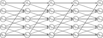
Could the same strategy that works for the sequential model also be used for representing Goldbeter’s dynamical model by using causal graphs? Indeed, it could be suggested that the causal structure of the model is captured by figure 1.
Proposed time-indexed DAG representing the causal dependencies in the Goldbeter model. The vertices of the graph represent the concentrations of the different molecular species at different discrete time points, time moving from left to right.

It could be argued that this DAG contains all the causal relations posited by the Goldbeter model. But how can we incorporate the necessary quantitative information into this causal model? I suggest that this could be done by writing down rules for updating the values of the salient variables from each discrete time point to the next:


This iterative model computes, for each molecular species, the concentration increment from time t i to t i+1 = t i + Δt by approximating the exact time integral for the concentration function by M(t i) + ΔMΔt and for the other functions accordingly. In fact, this is also the standard approach to numerically integrating differential equations such as the ones that constitute the Goldbeter model, which have no analytic solution. In this approach, the Δt values can be made sufficiently small for the iterative model to be a good approximation for the continuous function.
This iterative model corresponds to the proposed causal graph (fig. 1) and appears to satisfy all the conditions for a structural causal model. Furthermore, the iterative model provides a way for numerically integrating the differential model devised by Goldbeter and thus for testing it. The system of differential equations as such is not analytically solvable and therefore cannot be used for making predictions. Thus, the differential Goldbeter model can only be tested with the help of the iterative model.
In any case, the iterative model shows that it is in principle possible to integrate dynamical information and causal difference-making information to some extent. As we have seen, the structural equations of the iterative model represent the dynamics as well as the causal dependencies of the PER mechanisms. However, the iterative model suffers from at least three different drawbacks. First, it is an approximation and uses discrete time intervals instead of continuous time. While the time intervals can be made arbitrarily short, thus minimizing the prediction error, it remains a discrete-time model and a coarse-grained description of reality. The causal structure shown in figure 1 may only show up in this coarse-grained picture. Second, the time derivatives of the concentration variables, which seem to play a crucial explanatory role in the differential model, have completely dropped out in the iterative model. This constitutes a potential loss of an explanatorily salient property. Third, the iterative model is derived with respect to the differential model, the latter being in this sense more fundamental. Furthermore, it is the differential model that explanatorily connects the mechanism to general theories of biophysical chemistry, in particular enzyme kinetics. If the formal approach could not represent the differential model itself, it would be missing a lot. Therefore, I now examine whether it could also be interpreted as a structural causal model.
3.5. The Differential Model Itself as a Structural Causal Model
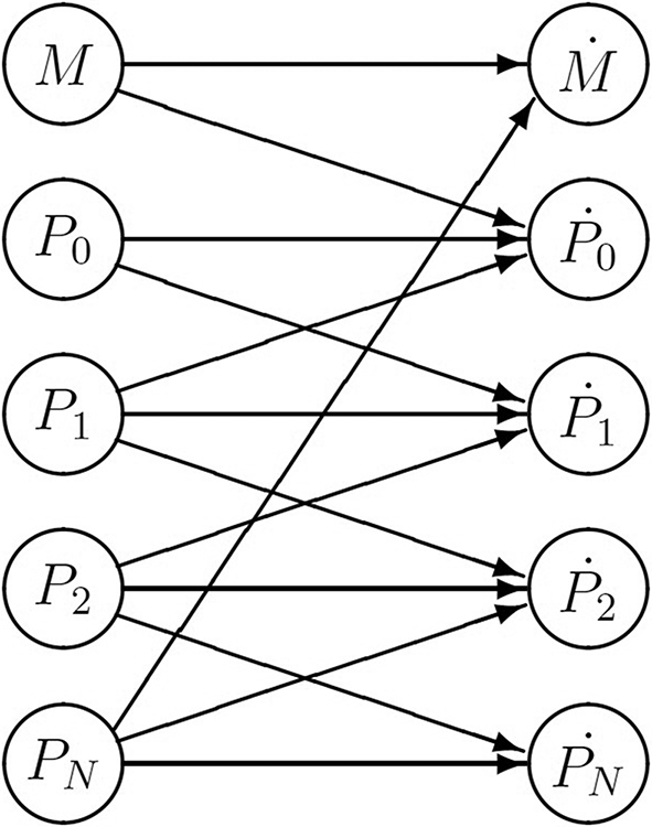
The question is now whether the differential equations constituting the Goldbeter model could themselves be interpreted as a structural causal model. The DAG associated with such a model, presumably, might look as shown in figure 2.
Proposed DAG for the differential model. The dots on the variables indicate time derivatives.

Interpreting Goldbeter’s equations causally in the way indicated in figure 2 requires that we can somehow write the equations in the form of structural equations, for example, in the sense of Pearl (Reference Pearl2000). That this cannot be done straightforwardly should be clear from the fact that such an equation requires exogenous variables, that is, variables that are controlled from outside the mechanism. Mathematically, a variable in a set of equations may be considered as exogenous if its time derivative does not depend on any other variable in the system. Obviously, none of the concentration variables in the Goldbeter model satisfy this requirement. Thus, at least some of the equations need to be replaced. In fact, several techniques have been published in the machine learning literature for deriving causal graphs and structural equations from differential equations.
A classical approach is the causal ordering algorithm developed by Herbert Simon. Using this approach, Iwasaki and Simon (Reference Iwasaki and Simon1994) propose two strategies for inferring causal relations from differential equations, namely, “equilibrating” and “exogenizing.” The first method is available for systems that contain equations that restore equilibrium very quickly after a disturbance compared to other equations. The second method may work when there are equations that change so slowly compared to the others that they may be replaced by a fixed value. There are several reasons why none of these approaches give a satisfactory solution for the Goldbeter model. First, there are no equations that change at a significantly different rate. In particular, the dynamic equilibrium is characterized by all concentration variables oscillating at the same frequency. Second, these techniques introduce approximations and idealizations of their own and will thus be subject to the same limitations as my iterative solution from the previous section.
Another technique consists in introducing brute-force interventions by setting time derivatives to zero and the corresponding variable to a fixed value (e.g., Mooij, Janzing, and Schölkopf Reference Mooji, Janzing and Schölkopf2013). In this approach, at least one of the equations in a system of differential equations dX i/dt = f i(X i) is replaced by an equation of the form X i = ξ i, where ξ i is a constant (thus dX i/dt = 0). This is the equivalent of an ideal intervention in ordinary structural equations. What this yields are structural equations describing static equilibrium states for the system as well as the effects that setting variables to fixed values has on these equilibrium states. Any dynamical behavior (i.e., behavior where the system still undergoes change) is thus lost, including in particular the dynamic equilibria.Footnote 2 Thus, these structural models do not represent the causal relations that operate while the system is undergoing change; they merely represent the effects that certain interventions have on a system that has been frozen in some state.
Are these limitations just inherent in the methods used by causal modelers so far, or are there fundamental reasons for thinking that some differential equation models resist a full representation as structural causal models? I will argue now that the latter is the case.
The main problem is that the Goldbeter equations do not have the right modularity properties that are required by structural causal models. Modularity requires that it be possible to intervene on each one of the equations that describe a causal structure without changing any other equations (Woodward Reference Woodward2003, 48–49, 327–39). The question of whether modularity is a necessary feature of any causal model has been debated; several authors have presented counterexamples (e.g., Cartwright Reference Cartwright, Galavotti, Suppes and Costantini2001; Mitchell Reference Mitchell2009). Kuorikoski (Reference Kuorikoski2012) has shown that any causal model must at least be modular in variables. This means that an intervention on one of the cause variables must not change the parameter set or the functional forms of the equations in the model. Failure of variable modularity prevents any prediction of the effects of the intervention, which is the raison d’être of a causal model according to interventionism. Without such predictions, the causal model cannot answer “what if things had been different” questions. But the ability to answer such questions is what defines a model as causal according to the interventionist approach.
I claim that the differential Goldbeter model lacks variable modularity. To see this, consider, for example, equations (1b) and (1c). Suppose we wished to intervene on P 0 in equation (1c) in order to manifest the causal dependence of dP 1/dt on P 0. We could try to set P 0 to an exogenously determined value ξ 0 and keep it fixed at this value. But to do this, we would have to set dP 0/dt = 0 and thus wipe out equation (1b), which constitutes a violation of (variable) modularity. Also, this would freeze the system in a static equilibrium and thus obliterate the explanandum phenomenon (circadian oscillation). Alternatively, we could try to push P 0 to some value ξ 0 at some time t 0 (e.g., by adding protein) and then let it go and let equation (1b) determine the value of dP 0/dt for all t > t 0. Let’s call this a “push and let go” (PLG) intervention. While a PLG intervention might preserve the functional forms of the other equations, it would not enable us to predict the effect of this intervention because this would require an analytic solution to the differential equation system, which demonstrably doesn’t exist. Of course, we could use a numerical integration procedure to make the prediction, but this would mean that we would use the iterative and not the differential model in order to determine the causal structure. PLG interventions on the differential model itself do not provide any quantitative causal information. But this is the kind of information we would need to fully integrate the differential model with causal difference-making information.
The failure of modularity is even more dramatic for some other variables. For instance, suppose we wished to intervene on P N in equation (1a) such as to manipulate the value of dM/dt. This should manifest the causal feedback of the PER protein in the transcription of its own gene, which is a crucial feature of the model. But because we cannot manipulate P N independently of dP N/dt, we would have to either replace equation (1e) by a different equation, for example, dP N/dt = 0, thus freezing the system, or accept that dP N/dt is changed along to some value consistent with equation (1e) by a PLG intervention. Thus, once again, it would in principle not be determinable quantitatively what effect this intervention has on the subsequent evolution of the concentration variables by using only the differential model. These differential equations just don’t work like structural equations.
I suggest that this failure of variable modularity prohibits a full assimilation of the dynamical information provided in the differential model into the formal causal framework. Thus, formal causal models and dynamical equation models remain complementary but not fully compatible perspectives that both contribute to our understanding of the biological phenomena.
In the following section, I will consider the possible replies to my argument open to proponents of the formal approach to mechanisms.
4. Possible Replies on Behalf of the Formal Approach to Mechanisms
An obvious reply open to the structural causal modeler consists in denying that the differential equations are even contenders for representing causal dependencies. For starters, the differential equations express synchronic and not diachronic dependencies. Causation as traditionally understood is diachronic. In a similar vein, it can be argued that equations need to be integrated in order to predict or explain physical events. Surely, when we want to discuss the causal content of models such as Goldbeter’s, we have to consider suitably integrated forms of the equations. As the model cannot be analytically integrated, we have to consider an approximation such as the iterative model that I have discussed in section 3.4. Indeed, as we have seen, this model qualifies perfectly as a structural causal model. This model thus reveals all the causal relations that the dynamical mechanism contains, so all is well.
My answer to this reply is the following: If this is correct, then what is the differential Goldbeter model for? Is it just a set of equations that can be used to generate a causal model? If it has no causal content itself, as this reply contends, then what is its content? Perhaps it could be suggested that, indeed, the differential model itself makes no causal claims, but rather just states some lawful dependencies between the variables. While this would be an interesting claim (which I won’t try to defend here), it doesn’t seem to work in favor of the formal approach to mechanisms. For this seems to imply that there is something in the mechanism, something that is explanatorily salient, that the formal causal representations leave out. So the representation of the mechanism would be at best incomplete. This is the first horn of the dilemma that I outlined in the introduction.
The second horn arises if we try to consider the differential equations as directly targeting a set of causal dependencies after all. The problem with this, as I have shown, is the failure of variable modularity, which prevents a full representation of the differential equations as structural equations. Thus, the formal causal approach can at best consider the variables of the model as interrelated but not as causally dependent. But if this is true, then the formal approach misses out on some causal dependencies that make up the mechanism and is therefore also incomplete.
Thus, any way we cut the cake, the formal framework permits only a partial representation of the dynamical biological mechanism. It leaves out either noncausal explanatory relations or causal relations.Footnote 3
5. Conclusions
I have shown that information about the dynamics of biological mechanisms cannot always be fully assimilated into an interventionist formal causal framework. Even though approximate, discrete-time models succeed in integrating dynamical and causal difference-making information, the structural causal modeling approach leads to a dilemma when trying to account for certain differential equation models. Because these equations do not have the right modularity properties, they must be considered either as noncausal to begin with or as exhibiting a kind of causality not representable in the formal framework. In either case, the formal causal framework provides only a partial perspective on the mechanism.
To be fair, it must be acknowledged that some followers of the formal approach to causality and mechanisms, in particular Gebharter and Kaiser (Reference Gebharter, Kaiser, Kaiser, Scholl, Plenge and Hüttemann2014), admit from the outset that the formal models can provide only a partial perspective. Furthermore, some causal theorists such as Woodward (Reference Woodward2003) do not understand their framework as universal accounts of causality. Here, I hope to have provided additional justification for their caution in showing where exactly the limitations of the formal interventionist approach lie.