2 Problem formulation

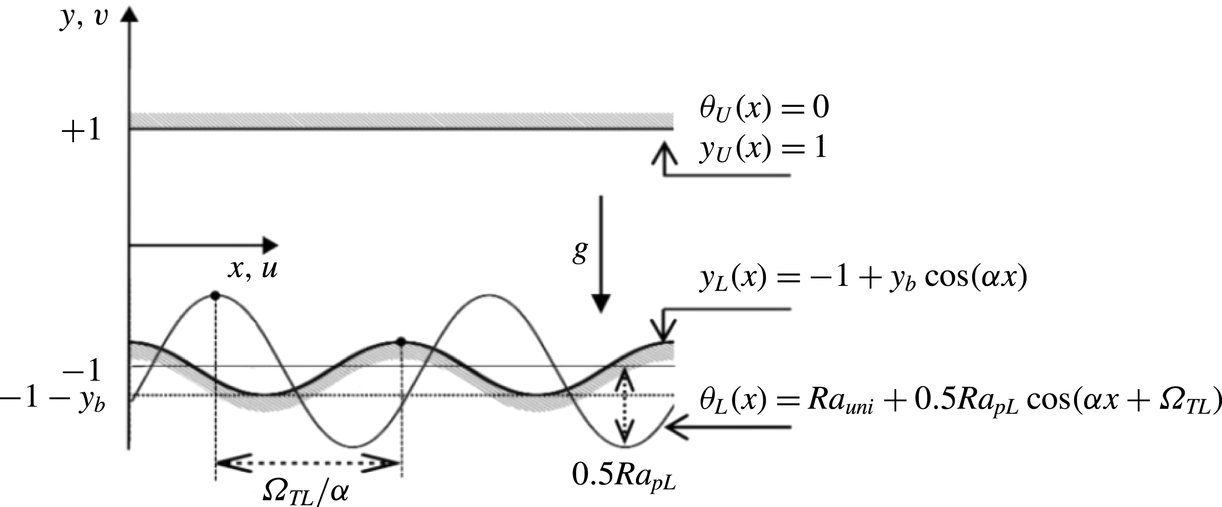
Consider a slot formed by two horizontal plates, the upper one being smooth and the lower one being corrugated (see figure 1), whose geometry has the following form:

(2.1a,b ) $$\begin{eqnarray}\displaystyle y_{L}^{\ast }(x^{\ast })=-h^{\ast }+C_{L}^{\ast }\cos (\unicode[STIX]{x1D6FC}^{\ast }x^{\ast }),\quad y_{U}^{\ast }(x^{\ast })=h^{\ast }. & & \displaystyle\end{eqnarray}$$

In the above, the subscripts $L$ and $U$ refer to the lower and upper plates, respectively, $C_{L}^{\ast }$ is the corrugation amplitude, $\unicode[STIX]{x1D6FC}^{\ast }$ is the corrugation wavenumber and stars denote dimensional quantities. The slot is periodic with a wavelength $\unicode[STIX]{x1D706}^{\ast }=2\unicode[STIX]{x03C0}/\unicode[STIX]{x1D6FC}^{\ast }$ and extends to $\pm \infty$ in the $x$ -direction, with $2h^{\ast }$ being the mean distance between the plates. The gravitational acceleration $g^{\ast }$ acts in the negative $y$ -direction, the fluid is incompressible, Newtonian, and has thermal conductivity $k^{\ast }$ , specific heat $c^{\ast }$ , thermal diffusivity $\unicode[STIX]{x1D705}^{\ast }=k^{\ast }/\unicode[STIX]{x1D70C}^{\ast }c^{\ast }$ , kinematic viscosity $\unicode[STIX]{x1D708}^{\ast }$ , dynamic viscosity $\unicode[STIX]{x1D707}^{\ast }$ , thermal expansion coefficient $\unicode[STIX]{x1D6E4}^{\ast }$ and variations of the density $\unicode[STIX]{x1D70C}^{\ast }$ follow the Boussinesq approximation.

Figure 1.

Schematic diagram of the flow system.

The upper plate is kept isothermal at temperature $T_{U}^{\ast }$ , which serves as the reference temperature, while the lower plate is subjected to a spatially distributed heating resulting in a sinusoidal distribution of its temperature ( $T_{L}^{\ast }$ ), i.e.

(2.2a,b ) $$\begin{eqnarray}\displaystyle T_{L}^{\ast }(x^{\ast })=T_{mean,L}^{\ast }+0.5T_{p,L}^{\ast }\cos (\unicode[STIX]{x1D6FC}^{\ast }x^{\ast }+\unicode[STIX]{x1D6FA}_{TL}^{\ast }),\quad T_{U}^{\ast }(x^{\ast })=T_{U}^{\ast }, & & \displaystyle\end{eqnarray}$$

where $T_{p,L}^{\ast }$ is the peak-to-peak amplitude of the periodic component and $\unicode[STIX]{x1D6FA}_{TL}^{\ast }$ is the phase shift between the heating and corrugation patterns.

We define the relative temperature as $\unicode[STIX]{x1D703}^{\ast }=T^{\ast }-T_{U}^{\ast }$ which leads to the plates’ temperatures of the form

(2.3a,b ) $$\begin{eqnarray}\displaystyle \unicode[STIX]{x1D703}_{L}^{\ast }(x)=\unicode[STIX]{x1D703}_{uni}^{\ast }+0.5\unicode[STIX]{x1D703}_{p,L}^{\ast }\cos (\unicode[STIX]{x1D6FC}^{\ast }x^{\ast }+\unicode[STIX]{x1D6FA}_{TL}^{\ast }),\quad \unicode[STIX]{x1D703}_{U}^{\ast }(x)=0, & & \displaystyle\end{eqnarray}$$

where $\unicode[STIX]{x1D703}_{uni}^{\ast }=T_{mean,L}^{\ast }-T_{U}^{\ast }$ , $\unicode[STIX]{x1D703}_{p,L}^{\ast }=T_{p,L}^{\ast }$ . Use of the half of the mean slot height $h^{\ast }$ as the length scale and $\unicode[STIX]{x1D705}^{\ast }\unicode[STIX]{x1D708}^{\ast }/(g^{\ast }\unicode[STIX]{x1D6E4}^{\ast }h^{\ast 3})$ as the temperature scale result in the following expressions for the geometry and temperatures

(2.4a,b ) $$\begin{eqnarray}\displaystyle y_{L}(x)=-1+y_{b}\cos (\unicode[STIX]{x1D6FC}x),\quad y_{U}(x)=1, & & \displaystyle\end{eqnarray}$$

(2.4c,d ) $$\begin{eqnarray}\displaystyle \unicode[STIX]{x1D703}_{L}(x)=Ra_{uni}+0.5Ra_{p,L}\cos (\unicode[STIX]{x1D6FC}x+\unicode[STIX]{x1D6FA}_{TL}),\quad \unicode[STIX]{x1D703}_{U}(x)=0, & & \displaystyle\end{eqnarray}$$

where $y_{b}$ is the amplitude of the corrugation, $Ra_{uni}=g^{\ast }\unicode[STIX]{x1D6E4}^{\ast }h^{\ast 3}\unicode[STIX]{x1D703}_{uni}^{\ast }/(\unicode[STIX]{x1D705}^{\ast }\unicode[STIX]{x1D708}^{\ast })$ and $Ra_{pL}=g^{\ast }\unicode[STIX]{x1D6E4}^{\ast }h^{\ast 3}\unicode[STIX]{x1D703}_{p,L}^{\ast }/(\unicode[STIX]{x1D705}^{\ast }\unicode[STIX]{x1D708}^{\ast })$ are the uniform and periodic Rayleigh numbers measuring the intensity of the uniform and periodic heating component.

The field equations consist of the continuity, Navier–Stokes and energy equations of the form

(2.5a,b ) $$\begin{eqnarray}\displaystyle \frac{\unicode[STIX]{x2202}u}{\unicode[STIX]{x2202}x}+\frac{\unicode[STIX]{x2202}v}{\unicode[STIX]{x2202}y}=0,\quad u\frac{\unicode[STIX]{x2202}u}{\unicode[STIX]{x2202}x}+v\frac{\unicode[STIX]{x2202}u}{\unicode[STIX]{x2202}y}=-\frac{\unicode[STIX]{x2202}p}{\unicode[STIX]{x2202}x}+\unicode[STIX]{x1D6FB}^{2}u, & & \displaystyle\end{eqnarray}$$

(2.5c,d ) $$\begin{eqnarray}\displaystyle u\frac{\unicode[STIX]{x2202}v}{\unicode[STIX]{x2202}x}+v\frac{\unicode[STIX]{x2202}v}{\unicode[STIX]{x2202}y}=-\frac{\unicode[STIX]{x2202}p}{\unicode[STIX]{x2202}y}+\unicode[STIX]{x1D6FB}^{2}v+Pr^{-1}\unicode[STIX]{x1D703},\quad u\frac{\unicode[STIX]{x2202}\unicode[STIX]{x1D703}}{\unicode[STIX]{x2202}x}+v\frac{\unicode[STIX]{x2202}\unicode[STIX]{x1D703}}{\unicode[STIX]{x2202}y}=Pr^{-1}\unicode[STIX]{x1D6FB}^{2}\unicode[STIX]{x1D703}, & & \displaystyle\end{eqnarray}$$

where ( $u$ , $v$ ) are the velocity components in the ( $x$ , $y$ ) directions, respectively, scaled with $U_{v}^{\ast }=\unicode[STIX]{x1D708}^{\ast }/h^{\ast }$ as the velocity scale, $p$ stands for the pressure scaled with $\unicode[STIX]{x1D70C}^{\ast }U_{\unicode[STIX]{x1D708}}^{\ast 2}$ as the pressure scale and $Pr=\unicode[STIX]{x1D708}^{\ast }/\unicode[STIX]{x1D705}^{\ast }$ is the Prandtl number. The relevant boundary conditions have the form

(2.6a-d ) $$\begin{eqnarray}\displaystyle u(y_{L})=u(1)=0,\quad v(y_{L})=v(1)=0,\quad \unicode[STIX]{x1D703}(y_{L})=\unicode[STIX]{x1D703}_{L}(x),\quad \unicode[STIX]{x1D703}(1)=0. & & \displaystyle\end{eqnarray}$$

There is no externally imposed horizontal pressure gradient, i.e.

(2.7) $$\begin{eqnarray}\displaystyle \left.\frac{\unicode[STIX]{x2202}p}{\unicode[STIX]{x2202}x}\right|_{mean}=0. & & \displaystyle\end{eqnarray}$$

System (2.5)–(2.7) is solved by expressing the velocity components using the stream function $\unicode[STIX]{x1D713}$ defined in the usual manner, i.e. $u=\unicode[STIX]{x2202}\unicode[STIX]{x1D713}/\unicode[STIX]{x2202}y$ , $v=-\unicode[STIX]{x2202}\unicode[STIX]{x1D713}/\unicode[STIX]{x2202}x$ , eliminating pressure and using Fourier expansions in the $x$ -direction and Chebyshev expansions in the $y$ -direction discretization combined with the immersed boundary conditions (IBC) method (Husain & Floryan Reference Husain and Floryan2010; Abtahi, Hossain & Floryan Reference Abtahi, Hossain and Floryan2016) to account for the irregularity of the flow domain. The pressure field is normalized with condition $p(0,0)=C$ , where $C$ represents an arbitrary constant.

The net flow rate $Q$ in the horizontal direction is defined as

(2.8) $$\begin{eqnarray}\displaystyle Q=\int _{y_{L}(x)}^{y_{U}(x)}u(x,y)\,\text{d}y. & & \displaystyle\end{eqnarray}$$

The surface stresses acting on the fluid at the lower plate $(\unicode[STIX]{x1D748}_{L})$ can be expressed as

(2.9) $$\begin{eqnarray}\displaystyle \unicode[STIX]{x1D748}_{L}=\left[\begin{array}{@{}cc@{}}\unicode[STIX]{x1D70E}_{x,L}, & \unicode[STIX]{x1D70E}_{y,L}\end{array}\right]=\left[\begin{array}{@{}cc@{}}n_{x,L}, & n_{y,L}\end{array}\right]\left[\begin{array}{@{}cc@{}}\unicode[STIX]{x1D70F}_{xx}-p & \unicode[STIX]{x1D70F}_{xy}\\ \unicode[STIX]{x1D70F}_{yx} & \unicode[STIX]{x1D70F}_{yy}-p\end{array}\right]_{y_{L}}, & & \displaystyle\end{eqnarray}$$

where

(2.10a-c ) $$\begin{eqnarray}\displaystyle \unicode[STIX]{x1D70F}_{xx}=2\frac{\unicode[STIX]{x2202}u}{\unicode[STIX]{x2202}x},\quad \unicode[STIX]{x1D70F}_{xy}=\unicode[STIX]{x1D70F}_{yx}=\frac{\unicode[STIX]{x2202}u}{\unicode[STIX]{x2202}y}+\frac{\unicode[STIX]{x2202}v}{\unicode[STIX]{x2202}x},\quad \unicode[STIX]{x1D70F}_{yy}=2\frac{\unicode[STIX]{x2202}v}{\unicode[STIX]{x2202}y}, & & \displaystyle\end{eqnarray}$$

denote viscous components of the stress tensor and

(2.11) $$\begin{eqnarray}\displaystyle [n_{x,L},n_{y,L}]=N_{L}[-\unicode[STIX]{x1D6FC}y_{b}\sin (\unicode[STIX]{x1D6FC}x),-1] & & \displaystyle\end{eqnarray}$$

are components of the normal unit vector with $N_{L}=[1+(\unicode[STIX]{x1D6FC}y_{b}\sin (\unicode[STIX]{x1D6FC}x))^{2}]^{-1/2}$ . The $x$ - and $y$ -components of surface stresses are

(2.12a ) $$\begin{eqnarray}\displaystyle & \displaystyle \unicode[STIX]{x1D70E}_{x,L}=\unicode[STIX]{x1D70E}_{xv,L}+\unicode[STIX]{x1D70E}_{xp,L}=N_{L}\left[-2\unicode[STIX]{x1D6FC}y_{b}\sin (\unicode[STIX]{x1D6FC}x)\frac{\unicode[STIX]{x2202}u}{\unicode[STIX]{x2202}x}-\left(\frac{\unicode[STIX]{x2202}u}{\unicode[STIX]{x2202}y}+\frac{\unicode[STIX]{x2202}v}{\unicode[STIX]{x2202}x}\right)\right]_{y_{L}}+N_{L}[\unicode[STIX]{x1D6FC}y_{b}\sin (\unicode[STIX]{x1D6FC}x)p]_{y_{L}}, & \displaystyle \nonumber\\ \displaystyle & & \displaystyle\end{eqnarray}$$

(2.12b ) $$\begin{eqnarray}\displaystyle & \displaystyle \unicode[STIX]{x1D70E}_{y,L}=\unicode[STIX]{x1D70E}_{yv,L}+\unicode[STIX]{x1D70E}_{yp,L}=N_{L}\left[-\unicode[STIX]{x1D6FC}y_{b}\sin (\unicode[STIX]{x1D6FC}x)\left(\frac{\unicode[STIX]{x2202}u}{\unicode[STIX]{x2202}y}+\frac{\unicode[STIX]{x2202}v}{\unicode[STIX]{x2202}x}\right)-2\frac{\unicode[STIX]{x2202}v}{\unicode[STIX]{x2202}y}\right]_{y_{L}}+N_{L}[p]_{y_{L}},\quad & \displaystyle\end{eqnarray}$$

$\unicode[STIX]{x1D70E}_{xv,L}$

$\unicode[STIX]{x1D70E}_{yv,L}$

$\unicode[STIX]{x1D70E}_{xp,L}$

$\unicode[STIX]{x1D70E}_{yp,L}$

$x$

(2.13a ) $$\begin{eqnarray}\displaystyle & \displaystyle F_{x,L}=F_{xv,L}+F_{xp,L}=\unicode[STIX]{x1D706}^{-1}\int _{0}^{\unicode[STIX]{x1D706}}(\unicode[STIX]{x1D70E}_{xv,L}+\unicode[STIX]{x1D70E}_{xp,L})N_{L}^{-1}\,\text{d}x, & \displaystyle\end{eqnarray}$$

(2.13b ) $$\begin{eqnarray}\displaystyle & \displaystyle F_{y,L}=F_{yv,L}+F_{yp,L}=\unicode[STIX]{x1D706}^{-1}\int _{0}^{\unicode[STIX]{x1D706}}(\unicode[STIX]{x1D70E}_{yv,L}+\unicode[STIX]{x1D70E}_{yp,L})N_{L}^{-1}\,\text{d}x. & \displaystyle\end{eqnarray}$$

Similar relations can be developed for the upper plate. The corresponding conduction problem has been solved when necessary using methods described in Husain & Floryan (Reference Husain and Floryan2007).

3 Flow patterns

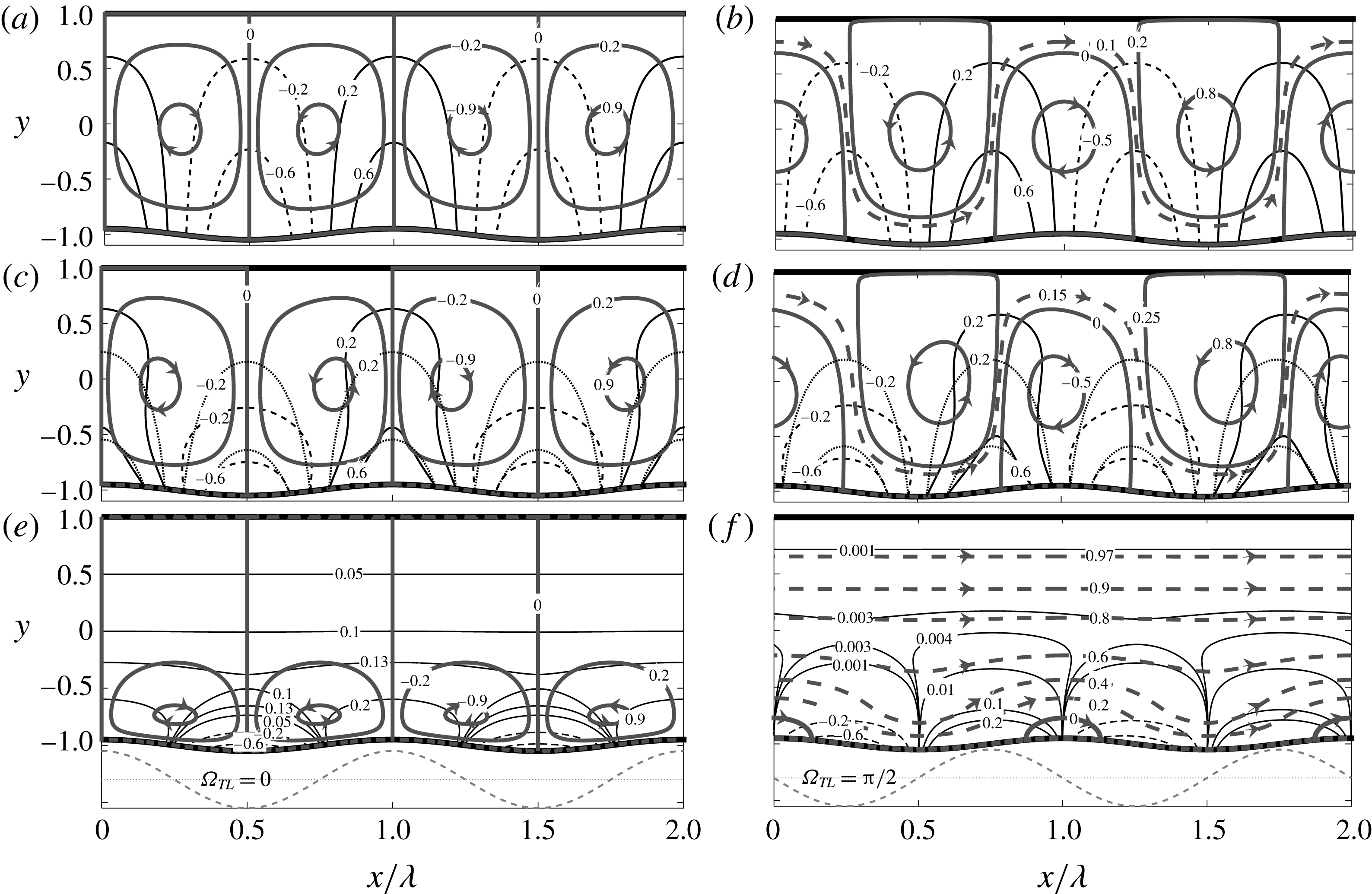
Typical flow patterns created by convection are displayed in figure 2. Figure 2(a,c,e) displays flow resulting from the hot spots at the lower wall overlapping with the corrugation peaks ( $\unicode[STIX]{x1D6FA}_{TL}=0$ ). The resulting topology consists of pairs of counter-rotating rolls with the fluid moving upwards above the hot spots. Figure 2(b,d,f) displays patterns for $\unicode[STIX]{x1D6FA}_{TL}=\unicode[STIX]{x03C0}/2$ with the flow topology consisting of sets of rolls separated from each other by a stream tube weaving up and down and carrying fluid in the positive $x$ -direction. All upper rolls rotate in the same direction and all lower rolls rotate in the direction opposite to the direction of the upper rolls.

Figure 2.

The flow (thick solid lines for the individual rolls and thick dashed lines for the stream tube) and the temperature (thin solid lines for the positive values and dashed lines for the negative values) fields for $Ra_{pL}=400,Ra_{uni}=0$ , $y_{b}=0.05$ and $\unicode[STIX]{x1D6FC}=0.01$ , 1.22, 8 for $\unicode[STIX]{x1D6FA}_{TL}=0$ (a,c,e) and for $\unicode[STIX]{x1D6FA}_{TL}=\unicode[STIX]{x03C0}/2$ (b,d,f). $\unicode[STIX]{x1D713}$ has been normalized with its maxima; $|\unicode[STIX]{x1D713}|_{max}=0.0591$ , 2.9634, 0.0351 in (a,c,e) and $0.0718$ , 3.6305, 0.1886 in (b,d,f) for $\unicode[STIX]{x1D6FC}=0.01$ , 1.22, 8, respectively. Temperature has been normalized with $\unicode[STIX]{x1D703}_{max}=Ra_{pL}/2$ . Dotted lines show conductive isotherms but which are different from the complete isotherms only for $\unicode[STIX]{x1D6FC}=1.22$ . Dashed lines illustrate temperatures of the lower plate.

In the next section, we begin detailed description of the mechanics of convection by starting with an analytic solution for the long-wavelength system.

4 The long-wavelength system

We begin detailed description of the mechanics of convection by starting with the long-wavelength system, i.e. $\unicode[STIX]{x1D6FC}\rightarrow 0$ . Solution begins with domain transformation of the form

(4.1a,b ) $$\begin{eqnarray}\displaystyle \unicode[STIX]{x1D709}=\unicode[STIX]{x1D6FC}x,\quad \unicode[STIX]{x1D702}=2\frac{y-1}{2-y_{b}\cos \unicode[STIX]{x1D709}}+1, & & \displaystyle\end{eqnarray}$$

where $\unicode[STIX]{x1D709}$ is a slow scale and $\unicode[STIX]{x1D702}$ maps the corrugated slot into a regular strip $\unicode[STIX]{x1D702}\in [-1,1]$ . The unknowns are represented as power expansions in terms of $\unicode[STIX]{x1D6FC}$ of the form

(4.2a ) $$\begin{eqnarray}\displaystyle [u,v,\unicode[STIX]{x1D703}]=[u_{0},v_{0},\unicode[STIX]{x1D703}_{0}]+\unicode[STIX]{x1D6FC}[u_{1},v_{1},\unicode[STIX]{x1D703}_{1}]+\unicode[STIX]{x1D6FC}^{2}[u_{2},v_{2},\unicode[STIX]{x1D703}_{2}]+O(\unicode[STIX]{x1D6FC}^{3}), & & \displaystyle\end{eqnarray}$$

(4.2b,c ) $$\begin{eqnarray}\displaystyle p=\unicode[STIX]{x1D6FC}^{-1}p_{-1}+p_{0}+\unicode[STIX]{x1D6FC}p_{1}+O(\unicode[STIX]{x1D6FC}^{2}),\quad Q=Q_{0}+\unicode[STIX]{x1D6FC}Q_{1}+\unicode[STIX]{x1D6FC}^{2}Q_{2}+O(\unicode[STIX]{x1D6FC}^{3}), & & \displaystyle\end{eqnarray}$$

these expansions are substituted into the field equations, the leading-order systems are extracted and solved with details given in appendix A. The solutions have the following forms:

(4.3) $$\begin{eqnarray}\displaystyle \left.\begin{array}{@{}c@{}}\displaystyle u_{0}=0,\quad v_{0}=0,\quad p_{-1}=0,\\ \displaystyle \unicode[STIX]{x1D703}_{0}=Ra_{uni}{\textstyle \frac{1}{2}}(1-\unicode[STIX]{x1D702})+Ra_{PL}{\textstyle \frac{1}{4}}(1-\unicode[STIX]{x1D702})(\cos \unicode[STIX]{x1D6FA}_{TL}\cos \unicode[STIX]{x1D709}-\sin \unicode[STIX]{x1D6FA}_{TL}\sin \unicode[STIX]{x1D709}),\quad Q_{0}=0,\end{array}\right\}\quad & & \displaystyle\end{eqnarray}$$

(4.4) $$\begin{eqnarray}\displaystyle \left.\begin{array}{@{}rcl@{}}\displaystyle v_{1}\; & =\; & 0,\quad \unicode[STIX]{x1D703}_{1}=0,\\ u_{1}\; & =\; & Ra_{uni}Pr^{-1}\displaystyle \mathop{\sum }_{n=0}^{3}LS_{u1,n}\sin (n\unicode[STIX]{x1D709})\\ \; & \; & \displaystyle +\,Ra_{pL}Pr^{-1}\mathop{\sum }_{n=0}^{3}[KS_{u1,n}\cos \unicode[STIX]{x1D6FA}_{TL}\sin (n\unicode[STIX]{x1D709})+KC_{u1,n}\sin \unicode[STIX]{x1D6FA}_{TL}\cos (n\unicode[STIX]{x1D709})],\\ \displaystyle p_{0}\; & =\; & Ra_{uni}Pr^{-1}[L_{p0}+LC_{p0,1}\cos (\unicode[STIX]{x1D709})]\\ \; & \; & \displaystyle +\,Ra_{pL}Pr^{-1}\mathop{\sum }_{n=0}^{2}[KS_{p0,n}\sin \unicode[STIX]{x1D6FA}_{TL}\sin (n\unicode[STIX]{x1D709})+KC_{p0,n}\cos \unicode[STIX]{x1D6FA}_{TL}\cos (n\unicode[STIX]{x1D709})]+C,\\ \displaystyle Q_{1}\; & =\; & Ra_{PL}Pr^{-1}K_{Q1}\sin \unicode[STIX]{x1D6FA}_{TL},\end{array}\right\}\quad & & \displaystyle\end{eqnarray}$$

(4.5) $$\begin{eqnarray}\displaystyle \left.\begin{array}{@{}rcl@{}}\displaystyle u_{2}\; & =\; & 0,\quad P_{1}=0,\\ v_{2}\; & =\; & Ra_{uni}Pr^{-1}\displaystyle \mathop{\sum }_{n=0}^{4}LC_{v2,n}\cos (n\unicode[STIX]{x1D709})+Ra_{pL}Pr^{-1}\mathop{\sum }_{n=0}^{4} [\!KS_{v2,n}\sin \unicode[STIX]{x1D6FA}_{TL}\sin (n\unicode[STIX]{x1D709})\\ \; & \; & \displaystyle +\,\cos \unicode[STIX]{x1D6FA}_{TL}\cos (n\unicode[STIX]{x1D709})\!],\\ \unicode[STIX]{x1D703}_{2}\; & =\; & Ra_{uni}Pr^{-1}\displaystyle \mathop{\sum }_{n=0}^{5}L1C_{\unicode[STIX]{x1D703}2,n}\cos (n\unicode[STIX]{x1D709})+Ra_{uni}^{2}Pr^{-1}\mathop{\sum }_{n=0}^{5}L2C_{\unicode[STIX]{x1D703}2,n}\cos (n\unicode[STIX]{x1D709})\\ \; & \; & \displaystyle +\,Ra_{pL}Pr^{-1}\mathop{\sum }_{n=0}^{6}[K1S_{\unicode[STIX]{x1D703}2,n}\sin \unicode[STIX]{x1D6FA}_{TL}\sin (n\unicode[STIX]{x1D709})+K1C_{\unicode[STIX]{x1D703}2,n}\cos \unicode[STIX]{x1D6FA}_{TL}\cos (n\unicode[STIX]{x1D709})]\\ \; & \; & \displaystyle +\,Ra_{pL}^{2}Pr^{-1}\mathop{\sum }_{n=0}^{6}[K2S_{\unicode[STIX]{x1D703}2,n}\sin \unicode[STIX]{x1D6FA}_{TL}\sin (n\unicode[STIX]{x1D709})+K2C_{\unicode[STIX]{x1D703}2,n}\cos \unicode[STIX]{x1D6FA}_{TL}\cos (n\unicode[STIX]{x1D709})],\\ \displaystyle Q_{2}\; & =\; & 0,\end{array}\right\} & & \displaystyle\end{eqnarray}$$

with all coefficients defined in appendix A.

The structure of (4.3)–(4.5) demonstrates that in the limit of $Ra_{pL}\rightarrow 0$ the boundaries between the rolls overlap with the peaks and bottoms of the corrugation (Abtahi & Floryan Reference Abtahi and Floryan2017). Taking an additional limit of $y_{b}\rightarrow 0$ eliminates convection altogether if $Ra_{uni}<213.5$ (Chandrasekhar Reference Chandrasekhar1961). In the limit of $Ra_{uni}\rightarrow 0,y_{b}\rightarrow 0$ the locations of the boundaries overlap with the locations of the hot and cold spots at the lower wall (Hossain & Floryan Reference Hossain and Floryan2013a , Reference Hossain and Floryan2016; Asgarian, Hossain & Floryan Reference Asgarian, Hossain and Floryan2016). The same happens in the corrugated slot, as long as $y_{b}$ remains small enough, which is of interest in this analysis. This fact can be shown by looking at the flow structure close to the upper plate (see figure 2) where the flow field can be approximated by taking advantage of the simplifications available in the limit of $\unicode[STIX]{x1D702}\rightarrow 1$ , i.e.

(4.6) $$\begin{eqnarray}\displaystyle u_{1}(\unicode[STIX]{x1D702}) & = & \displaystyle -\frac{(\unicode[STIX]{x1D702}-1)}{15}y_{b}Pr^{-1}Ra_{uni}\sin \unicode[STIX]{x1D709}\nonumber\\ \displaystyle & & \displaystyle +\,\frac{(\unicode[STIX]{x1D702}-1)}{15}Pr^{-1}Ra_{pL}\left[-\frac{1}{8}y_{b}\sin \unicode[STIX]{x1D6FA}_{TL}-\sin (\unicode[STIX]{x1D6FA}_{TL}+\unicode[STIX]{x1D709})+\frac{1}{2}y_{b}\sin (\unicode[STIX]{x1D6FA}_{TL}+2\unicode[STIX]{x1D709})\right]\nonumber\\ \displaystyle & & \displaystyle +\,O[(\unicode[STIX]{x1D702}-1)^{2}],\end{eqnarray}$$

and searching for locations of zeros of the above expression. In the special cases of $\unicode[STIX]{x1D6FA}_{TL}=0,\unicode[STIX]{x03C0}$ , borders between rolls overlap with the peaks and bottoms of the corrugation, which also overlap with the hot and cold spots.

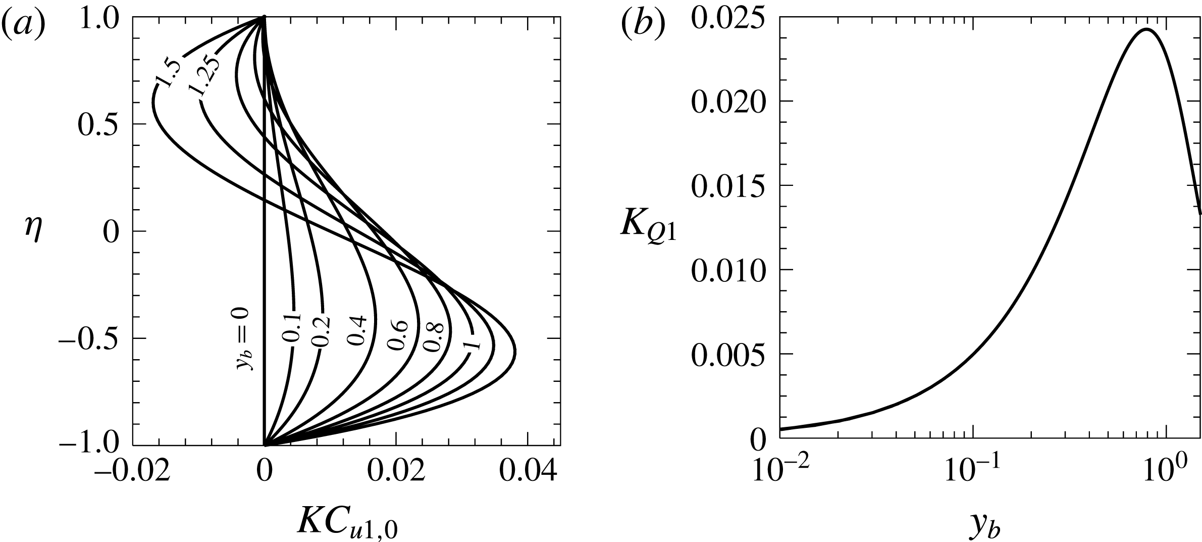
Equation (4.4) demonstrates that the velocity field has an aperiodic component in the horizontal direction, but only if there is a phase difference between the corrugation and heating patterns and this phase difference is not equal to $n\unicode[STIX]{x03C0}$ , where $n$ is an integer. The vertical distribution of this component is described by the function $KC_{u1,0}$ (see figure 3) and the corresponding volumetric flow rate is in general non-zero. We shall refer to the flow rate carried by this component as the thermal drift. The drift is independent of $Ra_{uni}$ , its magnitude is proportional to $Ra_{pL}$ , $Pr^{-1}$ and $\sin \unicode[STIX]{x1D6FA}_{TL}$ , and it disappears in the limit of $y_{b}\rightarrow 0$ as well as in the limit of $Ra_{pL}\rightarrow 0$ (see (4.4)), i.e. the presence of both the corrugation and the periodic heating is required for its generation. The drift disappears for $\unicode[STIX]{x1D6FA}_{TL}=0,\unicode[STIX]{x03C0}$ and changes direction when $\unicode[STIX]{x1D6FA}_{TL}$ traverses through any of these points. Since the drift is proportional to $\sin \unicode[STIX]{x1D6FA}_{TL}$ , this provides a simple means for control of its strength and direction through changes of the relative position of both patterns. The increase of the corrugation height initially increases the drift, but its excessive magnitude generates backflow near the upper plate (see figure 3) and reduces the flow rate.

Figure 3.

Distributions of the aperiodic component of the horizontal velocity, i.e. function $KC_{u1,0}$ (a) and variations of $Q$ (function $K_{Q1}$ ) as a function of $y_{b}$ (b) for the long-wavelength systems.

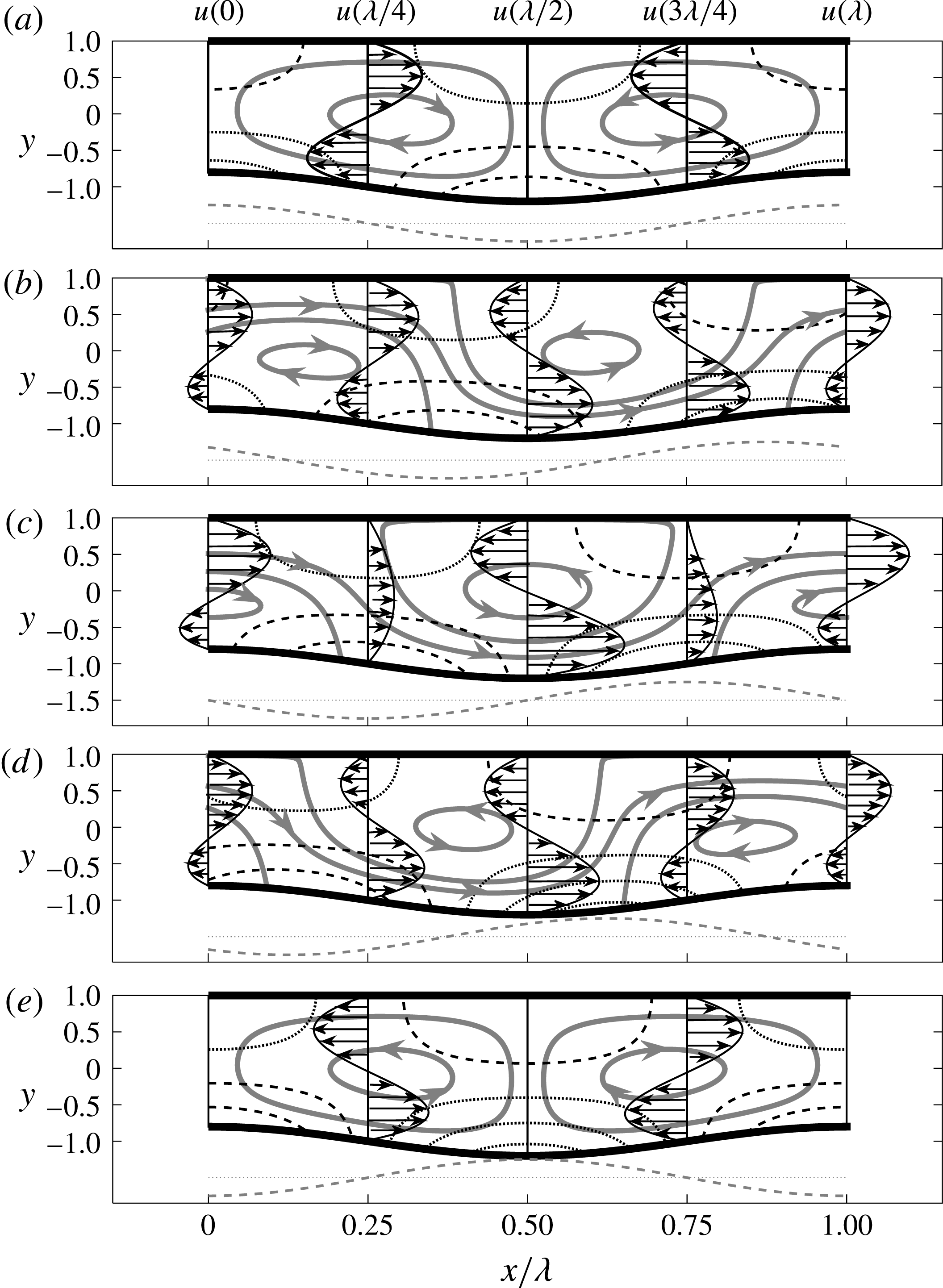
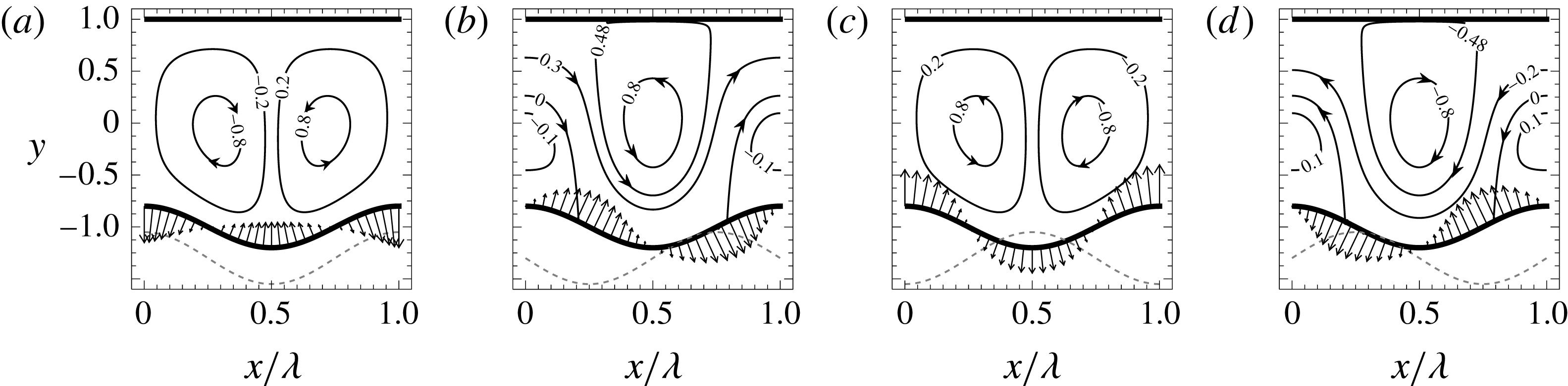
Figure 4 illustrates evolution of the flow field in response to changes of $\unicode[STIX]{x1D6FA}_{TL}$ . When $\unicode[STIX]{x1D6FA}_{TL}=0$ , the flow field consists of counter-rotating rolls with no mean flow in the horizontal direction, as the hot spots overlap with the corrugation peaks (figure 4 a). A jetting motion in the positive $x$ -direction appears when $\unicode[STIX]{x1D6FA}_{TL}=\unicode[STIX]{x03C0}/4$ , with the jet located close to the upper plate for $x\approx (-0.1\unicode[STIX]{x1D706},0.3\unicode[STIX]{x1D706})$ , then turning rapidly downwards at $x\approx 0.35\unicode[STIX]{x1D706}$ and staying close to the lower plate for $x\approx (0.4\unicode[STIX]{x1D706},0.8\unicode[STIX]{x1D706})$ and, finally, turning up at $x\approx 0.85\unicode[STIX]{x1D706}$ and staying close to the upper plate (see figure 4 b). The upward movement of the jet overlaps with the location of the hot spot and the downward movement overlaps with the location of the cold spot. The jet expands when $\unicode[STIX]{x1D6FA}_{TL}$ increases up to $\unicode[STIX]{x1D6FA}_{TL}=\unicode[STIX]{x03C0}/2$ and it occupies the complete cross-sections at $x\approx 0.25\unicode[STIX]{x1D706},0.75\unicode[STIX]{x1D706}$ with a nearly parabolic distribution of the horizontal velocity component (see figure 4 c). Further increase of $\unicode[STIX]{x1D6FA}_{TL}$ results in a decrease of the size of the jet and a change in the locations of the downward and upward turns, as illustrated in figure 4(d) for $\unicode[STIX]{x1D6FA}_{TL}=3\unicode[STIX]{x03C0}/4$ ; the former turn is now located at $x\approx 0.15\unicode[STIX]{x1D706}$ and the latter at $x\approx 0.65\unicode[STIX]{x1D706}$ . The jet disappears altogether at $\unicode[STIX]{x1D6FA}_{TL}=\unicode[STIX]{x03C0}/2$ , with the flow consisting of rolls rotating in the directions opposite to that found for $\unicode[STIX]{x1D6FA}_{TL}=0$ (see figure 4 e).

Figure 4.

Evolution of the flow field as a function of $\unicode[STIX]{x1D6FA}_{TL}$ for $y_{b}=0.2$ , $Ra_{pL}=400,Ra_{uni}=0,\unicode[STIX]{x1D6FC}\rightarrow 0$ . (a–e) Display results for $\unicode[STIX]{x1D6FA}_{TL}=0,\unicode[STIX]{x03C0}/4,\unicode[STIX]{x03C0}/2,3\unicode[STIX]{x03C0}/4,\unicode[STIX]{x03C0}$ , respectively. Thick solid lines identify streamlines. Thin dashed and dotted lines identify positive and negative pressures. Grey dashed–dotted line below each subfigure illustrates temperatures of the lower wall.

Appearance of the drift raises a question regarding the origin of forces responsible for its creation. As there is no mean horizontal pressure gradient, i.e. (2.7), the driving forces must be created at the plates. The upper plate is smooth and can only provide shear force which always opposes fluid movement. The lower plate generates both shear and pressure forces, with the former opposing the fluid movement. One can conclude that it is the pressure force which drives the mean horizontal flow.

Expressions for the $x$ -components of stresses acting on the fluid at both plates are given in appendix A. Their integration over one corrugation wavelength results in the following expressions for the forces acting on the fluid

(4.7a,b ) $$\begin{eqnarray}\displaystyle F_{xv,L}=-\unicode[STIX]{x1D6FC}y_{b}Pr^{-1}Ra_{pL}\sin \unicode[STIX]{x1D6FA}_{TL}k_{22}+O(\unicode[STIX]{x1D6FC}^{3}),\quad F_{xp,L}=\unicode[STIX]{x1D6FC}y_{b}Pr^{-1}Ra_{pL}\sin \unicode[STIX]{x1D6FA}_{TL}k_{23}+O(\unicode[STIX]{x1D6FC}^{3}), & & \displaystyle \nonumber\\ \displaystyle & & \displaystyle\end{eqnarray}$$

(4.7c,d ) $$\begin{eqnarray}\displaystyle F_{xv,U}=-\unicode[STIX]{x1D6FC}y_{b}Pr^{-1}Ra_{pL}\sin \unicode[STIX]{x1D6FA}_{TL}k_{24}+O(\unicode[STIX]{x1D6FC}^{3}),\quad F_{xp,U}=0, & & \displaystyle\end{eqnarray}$$

where the coefficients $k_{22}$ , $k_{23}$ , $k_{24}$ are defined in appendix A and are positive for $y_{b}<1$ . The above expressions demonstrate that the pressure represents the driving force which is opposed by viscous friction.

It is instructive to show in detail how the horizontal pressure force is created. The reader may note that the position of the corrugation is fixed but the position of the heating pattern is dictated by $\unicode[STIX]{x1D6FA}_{TL}$ . 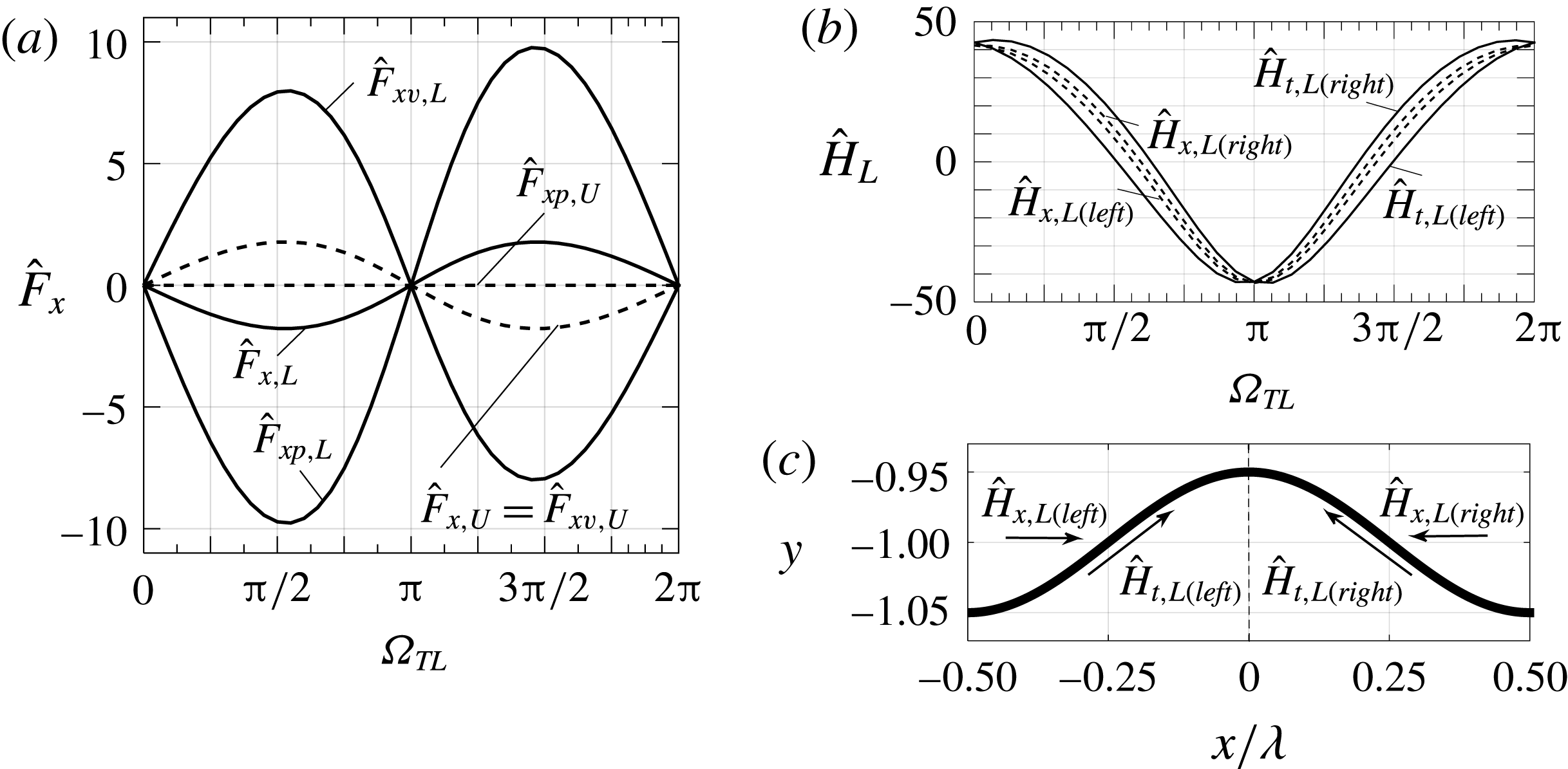Previous discussion shows that the location of the flow pattern is determined by the position of the heating pattern, and this location shifts in the horizontal direction when $\unicode[STIX]{x1D6FA}_{TL}$ changes. The process of changing the relative position of the pressure field with respect to the corrugation is illustrated in figure 5, which displays distributions of the pressure along the bottom plate. The reader may note that the direction of the drift changes from right to left due to changes of $\unicode[STIX]{x1D6FA}_{TL}$ (see figure 5(b,d) for $\unicode[STIX]{x1D6FA}_{TL}=\unicode[STIX]{x03C0}/2$ and $3\unicode[STIX]{x03C0}/2$ ).

Figure 5.

Distributions of pressure at the lower plate for $\unicode[STIX]{x1D6FC}\rightarrow 0$ , $y_{b}=0.2$ , $Ra_{pL}=400,Ra_{uni}=0$ and $\unicode[STIX]{x1D6FA}_{TL}=0,\unicode[STIX]{x03C0}/2,\unicode[STIX]{x03C0},3\unicode[STIX]{x03C0}/2$ in (a–d), respectively.

The evaluation of the horizontal pressure force, i.e.

(4.8) $$\begin{eqnarray}\displaystyle F_{xp,L} & = & \displaystyle \unicode[STIX]{x1D6FC}(2\unicode[STIX]{x03C0})^{-1}y_{b}\int _{0}^{2\unicode[STIX]{x03C0}}\sin \unicode[STIX]{x1D709}p_{0}|_{\unicode[STIX]{x1D702}=-1}\,\text{d}\unicode[STIX]{x1D709}\nonumber\\ \displaystyle & = & \displaystyle \unicode[STIX]{x1D6FC}(2\unicode[STIX]{x03C0}Pr)^{-1}y_{b}Ra_{uni}\int _{0}^{2\unicode[STIX]{x03C0}}\sin \unicode[STIX]{x1D709}[L_{p0}+LC_{p0,1}\cos \unicode[STIX]{x1D709}]_{\unicode[STIX]{x1D702}=-1}\,\text{d}\unicode[STIX]{x1D709}\nonumber\\ \displaystyle & & \displaystyle +\,\unicode[STIX]{x1D6FC}(2\unicode[STIX]{x03C0}Pr)^{-1}y_{b}Ra_{pL}\int _{0}^{2\unicode[STIX]{x03C0}}\sin \unicode[STIX]{x1D709}\mathop{\sum }_{n=0}^{2} [\!KS_{p0,n}\sin \unicode[STIX]{x1D6FA}_{TL}\sin (n\unicode[STIX]{x1D709})\nonumber\\ \displaystyle & & \displaystyle +\,KC_{p0,n}\cos \unicode[STIX]{x1D6FA}_{TL}\cos (n\unicode[STIX]{x1D709})]_{\unicode[STIX]{x1D702}=-1}\,\text{d}\unicode[STIX]{x1D709}\nonumber\\ \displaystyle & & \displaystyle +\,\unicode[STIX]{x1D6FC}(2\unicode[STIX]{x03C0})^{-1}Cy_{b}\int _{0}^{2\unicode[STIX]{x03C0}}\sin \unicode[STIX]{x1D709}\,\text{d}\unicode[STIX]{x1D709},\end{eqnarray}$$

shows that it can be viewed as a projection of the pressure field onto the geometry. This force has been referred to as the pressure interaction drag in the analysis of drag formation in grooved channels (Mohammadi & Floryan Reference Mohammadi and Floryan2012), but it acts as a propulsive force in the present case as it is created by an external effect, i.e. by the heating. Orthogonality properties of trigonometric functions lead to the final expression, which is identical to (4.7b ).

Shifting the relative position of the pressure field with respect to the corrugations results in different projections, different horizontal forces and different mean flow rates. The most effective projection resulting in the largest force and the largest drift corresponds to $\unicode[STIX]{x1D6FA}_{TL}=\pm \unicode[STIX]{x03C0}/2$ . The reader may note that a more complex corrugation geometry would lead to a more complex projection for the same heating pattern.

The horizontal forces at the upper and lower plates act in the opposite directions and this would lead to the relative movement of these plates if horizontal displacements were permitted. There would be no limit to the magnitude of this displacement as the force is dictated by the relative position of corrugation and heating pattern, which are unaltered by the plate movement; thus, the movement would persist as long as $\unicode[STIX]{x1D6FA}_{TL}\neq 0,\unicode[STIX]{x03C0}$ .

The horizontal forces acting on both sides of a single corrugation ‘bump’ are not the same and this may lead to ‘bump’ deformation if the plate was made of a soft material, e.g. biological membrane. Forces acting on the left ( ${\hat{H}}_{x,L(left)}$ ) and right ( ${\hat{H}}_{x,L(right)}$ ) sides of a single ‘bump’ are defined as

(4.9a,b ) $$\begin{eqnarray}\displaystyle \left.\begin{array}{@{}rcl@{}}{\hat{H}}_{x,L(left)}\; & =\; & -2\unicode[STIX]{x1D706}^{-1}\displaystyle \int _{-\unicode[STIX]{x1D706}/2}^{0}(\unicode[STIX]{x1D70E}_{xv,L}+\unicode[STIX]{x1D70E}_{xp,L})N_{L}^{-1}\,\text{d}x\\ \; & =\; & \displaystyle \frac{\unicode[STIX]{x1D6FC}}{5\unicode[STIX]{x03C0}Pr}[-y_{b}k_{25}Ra_{uni}+Ra_{pL}(k_{26}\cos \unicode[STIX]{x1D6FA}_{TL}-k_{27}\sin \unicode[STIX]{x1D6FA}_{TL})],\\ {\hat{H}}_{x,L(right)}\; & =\; & 2\unicode[STIX]{x1D706}^{-1}\displaystyle \int _{0}^{\unicode[STIX]{x1D706}/2}(\unicode[STIX]{x1D70E}_{xv,L}+\unicode[STIX]{x1D70E}_{xp,L})N_{L}^{-1}\,\text{d}x\\ \; & =\; & \displaystyle \frac{\unicode[STIX]{x1D6FC}}{5\unicode[STIX]{x03C0}Pr}[-y_{b}k_{25}Ra_{uni}+Ra_{pL}(k_{26}\cos \unicode[STIX]{x1D6FA}_{TL}+k_{27}\sin \unicode[STIX]{x1D6FA}_{TL})],\end{array}\right\} & & \displaystyle\end{eqnarray}$$

where the hat symbol has been added to mark forces acting on the plate as opposed to forces acting on the fluid, and all coefficients are defined in appendix A. Positive ${\hat{H}}_{x,L(left)}$ and ${\hat{H}}_{x,L(right)}$ are directed into the ‘bump’ and the difference between them defines the deforming force $\widehat{DF}_{x,L}$ , i.e.

(4.10) $$\begin{eqnarray}\displaystyle \widehat{DF}_{x,L} & = & \displaystyle {\hat{H}}_{x,L(left)}-{\hat{H}}_{x,L(right)}\nonumber\\ \displaystyle & = & \displaystyle -2\unicode[STIX]{x1D706}^{-1}\int _{-\unicode[STIX]{x1D706}/2}^{\unicode[STIX]{x1D706}/2}(\unicode[STIX]{x1D70E}_{xv,L}+\unicode[STIX]{x1D70E}_{xp,L})N_{L}^{-1}\,\text{d}x=-2(F_{xp,L}+F_{xv,L})\nonumber\\ \displaystyle & = & \displaystyle -2F_{x,L}=2\hat{F}_{x,L}=-\frac{2\unicode[STIX]{x1D6FC}}{5\unicode[STIX]{x03C0}Pr}k_{27}Ra_{pL}\sin \unicode[STIX]{x1D6FA}_{TL}\approx -0.05\frac{\unicode[STIX]{x1D6FC}}{Pr}y_{b}Ra_{pL}\sin \unicode[STIX]{x1D6FA}_{TL},\qquad\end{eqnarray}$$

which is equal and opposite to twice the net force acting on the fluid and is generated by the periodic heating.

We shall now inquire if the shear force would contribute to the corrugation buildup assuming erosion was allowed. This question is relevant as an accidental creation of a surface ripple could lead to its uncontrolled growth. Integration of tangential stress gives the total shear forces acting on the left $({\hat{H}}_{t,L(left)})$ and right $({\hat{H}}_{t,L(right)})$ sides of a single ‘bump’ (see appendix A for details). Positive ${\hat{H}}_{t,L(left)}$ and ${\hat{H}}_{t,L(right)}$ are directed towards the ‘bump’ peak which signals the tendency for the corrugation growth. We shall use simplified expressions valid for $y_{b}\rightarrow 0$ , i.e.

(4.11a,b ) $$\begin{eqnarray}\displaystyle \left.\begin{array}{@{}c@{}}\displaystyle {\hat{H}}_{t,L(right)}=\frac{\unicode[STIX]{x1D6FC}}{5\unicode[STIX]{x03C0}Pr}[y_{b}Ra_{uni}+Ra_{pL}(\cos \unicode[STIX]{x1D6FA}_{TL}+2.356y_{b}\sin \unicode[STIX]{x1D6FA}_{TL})],\\ \displaystyle {\hat{H}}_{t,L(left)}=\frac{\unicode[STIX]{x1D6FC}}{5\unicode[STIX]{x03C0}Pr}[y_{b}Ra_{uni}+Ra_{pL}(\cos \unicode[STIX]{x1D6FA}_{TL}-2.356y_{b}\sin \unicode[STIX]{x1D6FA}_{TL})],\end{array}\right\} & & \displaystyle\end{eqnarray}$$

which show that the uniform heating always contributes to the buildup. The periodic heating contributes only if the hot spots overlap with the upper part of the corrugation. Since only $Ra_{uni}<213.5$ is of interest in this analysis, the periodic part of the heating determines if the convection contributes to the buildup. It is interesting to note that ${\hat{H}}_{t,L(left)}$ and ${\hat{H}}_{t,L(right)}$ are not equal.

The above solution provides an acceptable accuracy for $\unicode[STIX]{x1D6FC}<0.1$ as determined through comparisons with the complete solution (details not shown).

5 Systems with an arbitrary wavenumber

The mechanics of convective processes has been explained in the previous section. We shall now inquire how the system responds when its wavelengths are comparable to the slot height. The relevant solutions have been obtained using a spectrally accurate numerical solution of the complete model equations (2.5)–(2.7) with the algorithm details given in (Husain & Floryan Reference Husain and Floryan2010; Abtahi et al. Reference Abtahi, Hossain and Floryan2016). The discussion begins with a purely periodic heating.

5.1 Slot exposed to a purely periodic heating $(Ra_{uni}\rightarrow 0)$

Results displayed in figure 2 demonstrate that the heating wavelength determines the topology of the flow field similarly as in the smooth slot (Hossain & Floryan Reference Hossain and Floryan2013b ). The rolls completely fill in the slot for long wavelengths (see in figure 2 a,b) but convection is very weak (see figure 6). Reduction of the wavelength down to $\unicode[STIX]{x1D6FC}=1.22$ (see in figure 2 c,d) results in an intensification of convection (see figure 6) with the rolls still completely filling in the slot. Further reduction of the wavelength down to $\unicode[STIX]{x1D6FC}=8$ (see in figure 2 e,f) results in a weakening of convection (see figure 6) with the fluid movement limited to a boundary layer adjacent to the corrugated plate; the thickness of this boundary layer rapidly decreases with increasing $\unicode[STIX]{x1D6FC}$ . Addition of a phase shift between the heating and corrugation patterns adds a stream tube carrying the fluid in the horizontal direction (compare figure 2 a–f). The stream tube expands as $\unicode[STIX]{x1D6FC}$ increases and it occupies around 90 % of slot volume at $\unicode[STIX]{x1D6FC}=8$ . 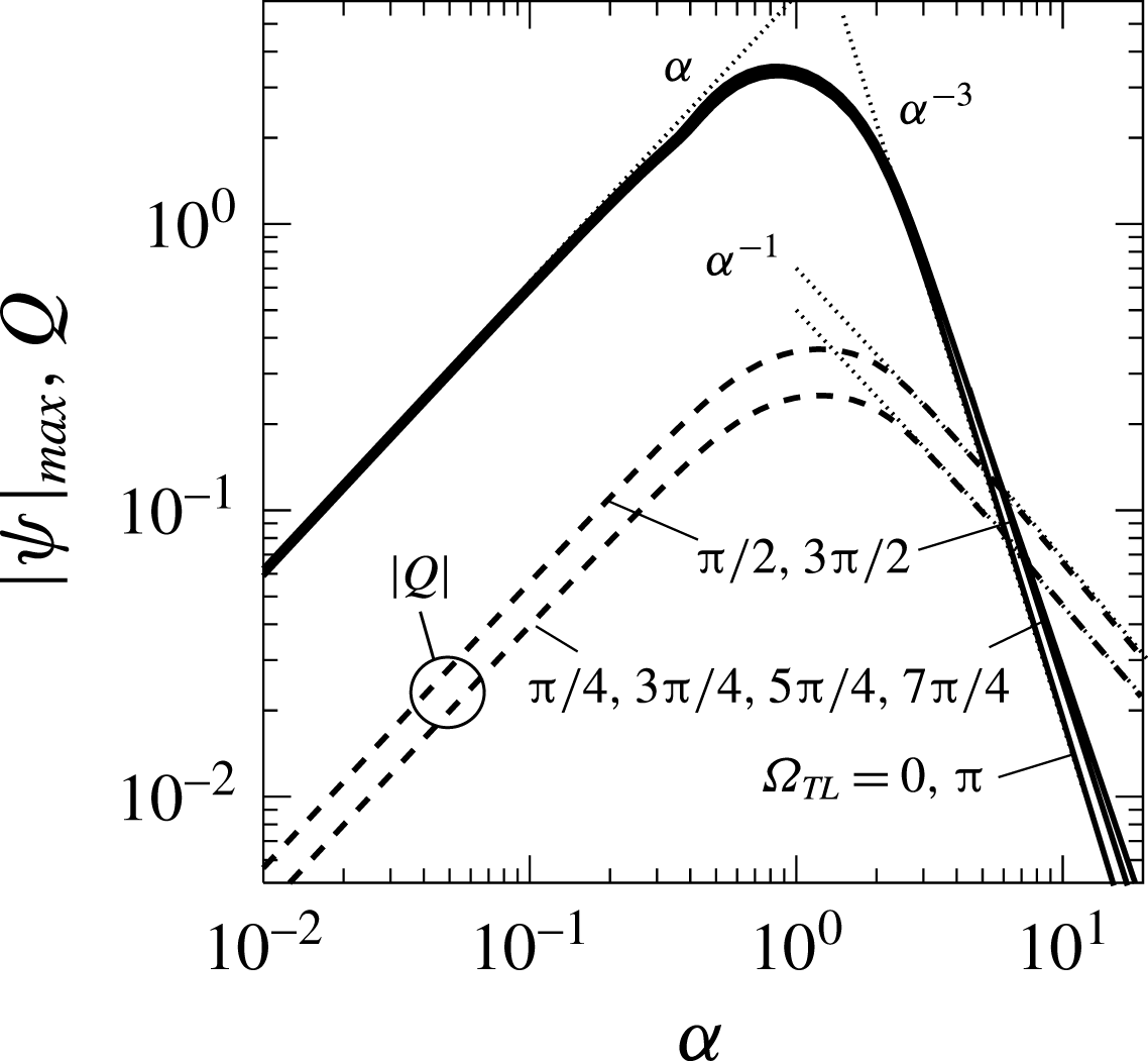There are two processes associated with convection and they lead to different values of $|\unicode[STIX]{x1D713}|_{max}$ (see figure 6). The first process is associated with rotation of rolls and locations of the corresponding $|\unicode[STIX]{x1D713}|_{max}$ overlaps with roll centres. The second process is associated with the formation of the stream tube and the relevant $|\unicode[STIX]{x1D713}|_{max}$ are located at the upper wall and their values give the flow rate $Q$ . Analysis carried out in § 4 shows that $|\unicode[STIX]{x1D713}|_{max}$ associated with the roll motion is dominant with $|\unicode[STIX]{x1D713}|_{max}=0(\unicode[STIX]{x1D6FC})$ for $\unicode[STIX]{x1D6FC}\rightarrow 0$ . At the same time, $Q=0(\unicode[STIX]{x1D6FC})$ , but only if $\unicode[STIX]{x1D6FA}_{TL}\neq 0,\unicode[STIX]{x03C0}$ , as $Q=0$ in these two special cases. Numerical estimates carried out for $\unicode[STIX]{x1D6FC}\rightarrow \infty$ (see Floryan & Floryan (Reference Floryan and Floryan2015), for methodology) show that $|\unicode[STIX]{x1D713}|_{max}$ associated with the roll motion decreases proportionally to $\unicode[STIX]{x1D6FC}^{-3}$ until it becomes small enough that it is overcome by $|\unicode[STIX]{x1D713}|_{max}$ associated with the formation of the stream tube. From that moment on, $|\unicode[STIX]{x1D713}|_{max}$ decreases at a rate proportional to $\unicode[STIX]{x1D6FC}^{-1}$ , as $Q=0(\unicode[STIX]{x1D6FC}^{-1})$ (see figure 6). The stream tube is not formed for $\unicode[STIX]{x1D6FA}_{TL}=0,\unicode[STIX]{x03C0}$ and in this case $|\unicode[STIX]{x1D713}|_{max}=0(\unicode[STIX]{x1D6FC}^{-3})$ . The maxima of $|\unicode[STIX]{x1D713}|_{max}$ and $Q$ occur at different values of $\unicode[STIX]{x1D6FC}$ and $\unicode[STIX]{x1D6FA}_{TL}$ ; in the case of conditions used in figures 6 and 7 they occur at $(\unicode[STIX]{x1D6FC},\unicode[STIX]{x1D6FA}_{TL})\approx (0.86,\unicode[STIX]{x03C0}/2),(1.22,\unicode[STIX]{x03C0}/2)$ , respectively.

Figure 6.

Variations of $|\unicode[STIX]{x1D713}|_{max}$ and $Q$ as functions of $\unicode[STIX]{x1D6FC}$ for $Ra_{pL}=400,Ra_{uni}=0,y_{b}=0.02.$ Thin dotted lines mark asymptotes. The maxima of $|\unicode[STIX]{x1D713}|_{max}$ and $Q$ occur at $(\unicode[STIX]{x1D6FC},\unicode[STIX]{x1D6FA}_{TL})\approx (0.86,\unicode[STIX]{x03C0}/2),(1.22,\unicode[STIX]{x03C0}/2)$ .

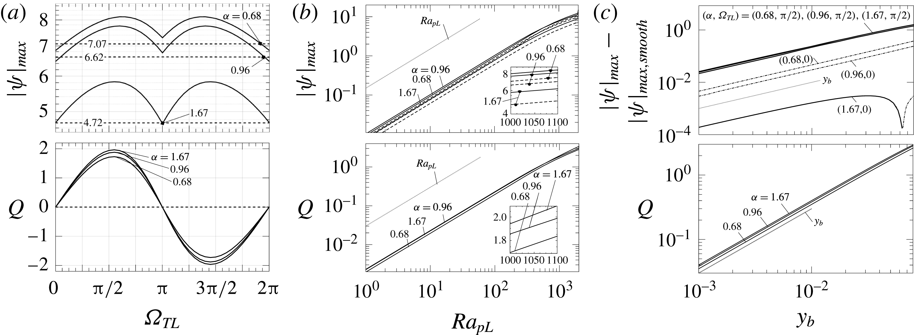
The convection intensity, as measured by $|\unicode[STIX]{x1D713}|_{max}$ , as well as the net flow rate $Q$ , display nearly sinusoidal variations as functions of $\unicode[STIX]{x1D6FA}_{TL}$ (see figure 7 a), including the change of direction of $Q$ between $\unicode[STIX]{x1D6FA}_{TL}\in (0,\unicode[STIX]{x03C0})$ and $\unicode[STIX]{x1D6FA}_{TL}\in (\unicode[STIX]{x03C0},2\unicode[STIX]{x03C0})$ . The maxima of $|\unicode[STIX]{x1D713}|_{max}$ occur approximately at $\unicode[STIX]{x1D6FA}_{TL}=\unicode[STIX]{x03C0}/2,3\unicode[STIX]{x03C0}/2$ , which also correspond to the maxima of $Q$ . Both $|\unicode[STIX]{x1D713}|_{max}$ and $Q$ increase proportionally to $Ra_{pL}$ , with a small reduction of the growth rate observed for $Ra_{pL}>10^{3}$ suggesting the beginning of a saturation process (see figure 7 b). The effect of an increase in $y_{b}$ is best represented by looking at the change with respect to convection in a smooth slot ( $y_{b}\rightarrow 0$ ) (Hossain & Floryan Reference Hossain and Floryan2013a ). The proper test quantity is thus $|\unicode[STIX]{x1D713}|_{max}-|\unicode[STIX]{x1D713}|_{max,smooth}$ for the stream function and $Q$ for the flow rate as $Q_{smooth}=0$ . Results displayed in figure 7(c) demonstrate a linear growth of both the convection intensity and the flow rate with $y_{b}$ for the range of corrugation amplitudes being of interest. This conclusion is supported by results of the analysis of the small- $y_{b}$ limit analysis presented in appendix B.

Figure 7.

Variations of $|\unicode[STIX]{x1D713}|_{max}$ and $Q$ as functions of $\unicode[STIX]{x1D6FA}_{TL}$ (a), $Ra_{pL}$ (b) and $y_{b}$ (c). The results are for $Ra_{uni}=0$ , $Pr=0.71$ , $y_{b}=0.05$ , $\unicode[STIX]{x1D6FA}_{TL}=\unicode[STIX]{x03C0}/2,Ra_{pL}=1000$ unless specified otherwise in the figure. Dashed lines correspond to the smooth slot and dotted lines identify various asymptotes. Dashed–dotted lines in (c) identify negative values. Wavenumbers $\unicode[STIX]{x1D6FC}=0.68$ , 1.67 produce maxima of $|\unicode[STIX]{x1D713}|_{max}$ , $Q$ , respectively.

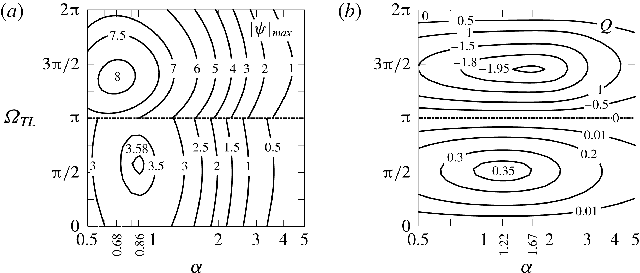
The effect of the phase difference is well illustrated in figure 8 for the range of $\unicode[STIX]{x1D6FC}$ producing the strongest convection. The results show that $|\unicode[STIX]{x1D713}|_{max}$ and $Q$ can be significantly altered by changing $\unicode[STIX]{x1D6FA}_{TL}$ . The maxima of these quantities do not occur for the same conditions, e.g. the maximum of $|\unicode[STIX]{x1D713}|_{max}$ and the maximum of $Q$ occur at $(\unicode[STIX]{x1D6FC},\unicode[STIX]{x1D6FA}_{TL})\approx (0.86,\unicode[STIX]{x03C0}/2),(1.22,\unicode[STIX]{x03C0}/2)$ , respectively, for flow conditions used in the lower half of figure 8. Increasing $Ra_{pL}$ from 400 to 1000 and $y_{b}$ from 0.02 to 0.05 moves these maxima to $(\unicode[STIX]{x1D6FC},\unicode[STIX]{x1D6FA}_{TL})\approx (0.68,2\unicode[STIX]{x03C0}/3),(1.67,\unicode[STIX]{x03C0}/2)$ , respectively (see the upper half of figure 8).

Figure 8.

Variations of $|\unicode[STIX]{x1D713}|_{max}$ (a) and $Q$ (b) as functions of $\unicode[STIX]{x1D6FC}$ and $\unicode[STIX]{x1D6FA}_{TL}$ for $Ra_{pL}=400,Ra_{uni}=0,y_{b}=0.02$ in the lower half of these figures and for $Ra_{pL}=1000,y_{b}=0.05$ in the upper half. Results can be extended to the full range of $\unicode[STIX]{x1D6FA}_{TL}$ by taking advantage of the periodicity in the $\unicode[STIX]{x1D6FA}_{TL}$ -direction.

Variations of forces acting on the plates as functions of $\unicode[STIX]{x1D6FA}_{TL}$ are illustrated in figure 9. Forces at each plate act in opposite directions, which may result in a relative horizontal translation of the plates if such an effect was permitted. There is no limit to the magnitude of such translation as forces persist as long as $\unicode[STIX]{x1D6FA}_{TL}\neq 0,\unicode[STIX]{x03C0}$ . The forces acting per one wavelength may not be large, but could become significant if integrated over several wavelengths. The same forces would contribute to the horizontal deformation of the corrugation if such an effect was allowed.

Figure 9.

Variations of the $x$ -component of forces acting on the plates (a; see (2.13) for definition) and forces acting on the right and left sides of the corrugation (b; see (4.9a,b )–(4.11a,b ) for definitions) as functions of $\unicode[STIX]{x1D6FA}_{TL}$ for $\unicode[STIX]{x1D6FC}=1.67,y_{b}=0.05,Ra_{pL}=1000,Ra_{uni}=0$ . In (a), solid (dashed) lines correspond to the lower (upper) plate. Hats above symbols signify forces acting on the plates. Directions of forces acting on the corrugation are shown in (c).

5.2 Placement of the corrugation and the heating at the upper plate

We shall now move the corrugations as well as the periodic heating to the upper plate. The proper boundary conditions have the following form

(5.1a,b ) $$\begin{eqnarray}\displaystyle u(-1)=u(y_{U})=0,\quad v(-1)=v(y_{U})=0, & & \displaystyle\end{eqnarray}$$

(5.1c,d ) $$\begin{eqnarray}\displaystyle \unicode[STIX]{x1D703}(-1)=0,\quad \unicode[STIX]{x1D703}(y_{U})=\unicode[STIX]{x1D703}_{U}(x)=0.5Ra_{pU}\cos (\unicode[STIX]{x1D6FC}x+\unicode[STIX]{x1D6FA}_{TU}), & & \displaystyle\end{eqnarray}$$

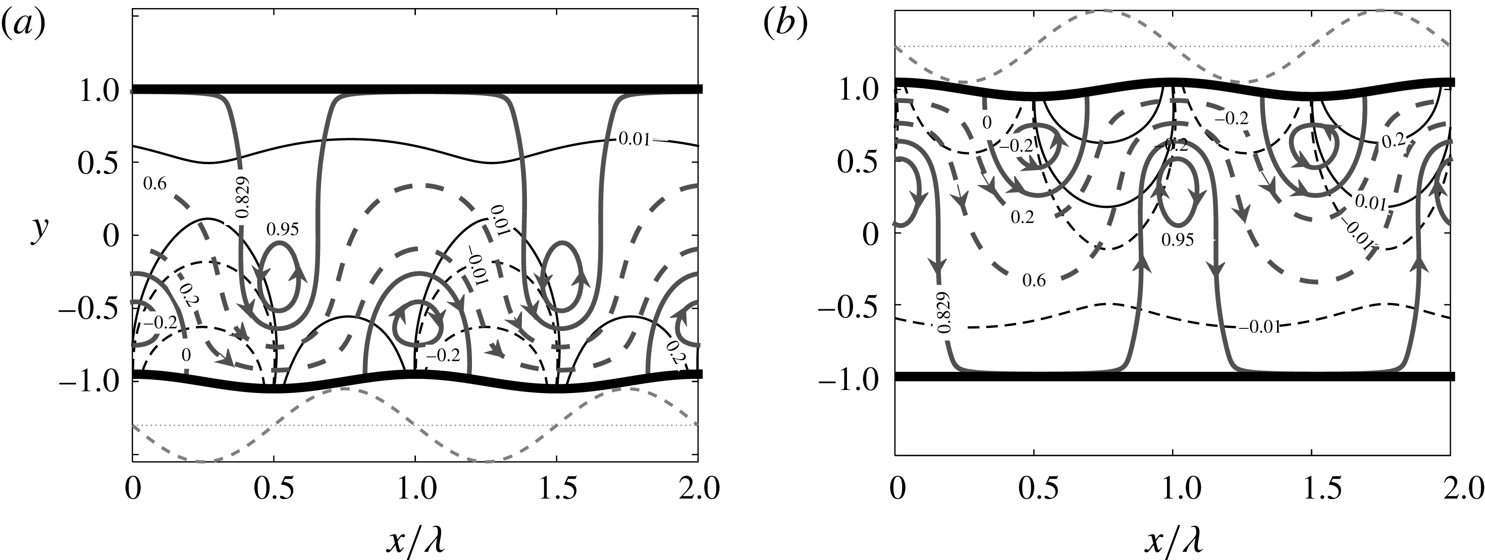
where $y_{U}(x)=1+y_{t}\cos (\unicode[STIX]{x1D6FC}x)$ and the field equations remain unchanged (see (2.5)). The resulting convection is analogous to convection resulting from the heating and corrugations placed at the lower plate. This similarity can be demonstrated by (i) reversing the direction of gravity, i.e. $Ra_{pU}\rightarrow -Ra_{pL}$ , and (ii) changing the sign of the temperature, i.e. $\unicode[STIX]{x1D703}\rightarrow -\unicode[STIX]{x1D703}$ (Hossain & Floryan Reference Hossain and Floryan2014). The latter condition implies a change of the sign of the temperature imposed at the lower plate and results in a shift of the temperature field by half of a cycle in the $x$ -direction. This similarity is illustrated in figure 10.

Figure 10.

The flow and temperature fields for $Ra_{uni}=0$ , $\unicode[STIX]{x1D6FA}_{TL}=\unicode[STIX]{x03C0}/2$ for heating and corrugations placed at the lower plate (a; $Ra_{pL}=400,Ra_{pU}=0$ , $\unicode[STIX]{x1D6FC}=4$ , $y_{b}=0.05$ , $y_{t}=0$ ) and at the upper plate (b; $Ra_{pL}=0,Ra_{pU}=400$ , $\unicode[STIX]{x1D6FC}=4$ , $y_{b}=0,y_{t}=0.05$ ). Thick solid, thick dashed, thin solid and thin dashed lines identify streamlines, stream tubes, positive isotherms and negative isotherms, respectively. $\unicode[STIX]{x1D713}$ and $\unicode[STIX]{x1D703}$ are normalized with their maxima; $|\unicode[STIX]{x1D713}|_{max}=0.5131$ , $\unicode[STIX]{x1D703}_{max}=Ra_{pL}/2$ for the lower plate heating and $\unicode[STIX]{x1D703}_{max}=Ra_{pU}/2$ for the upper plate heating. Dashed line below (a) illustrates temperature of the lower plate while dashed line above (b) illustrates temperature of the upper plate.

5.3 Effects of the uniform heating

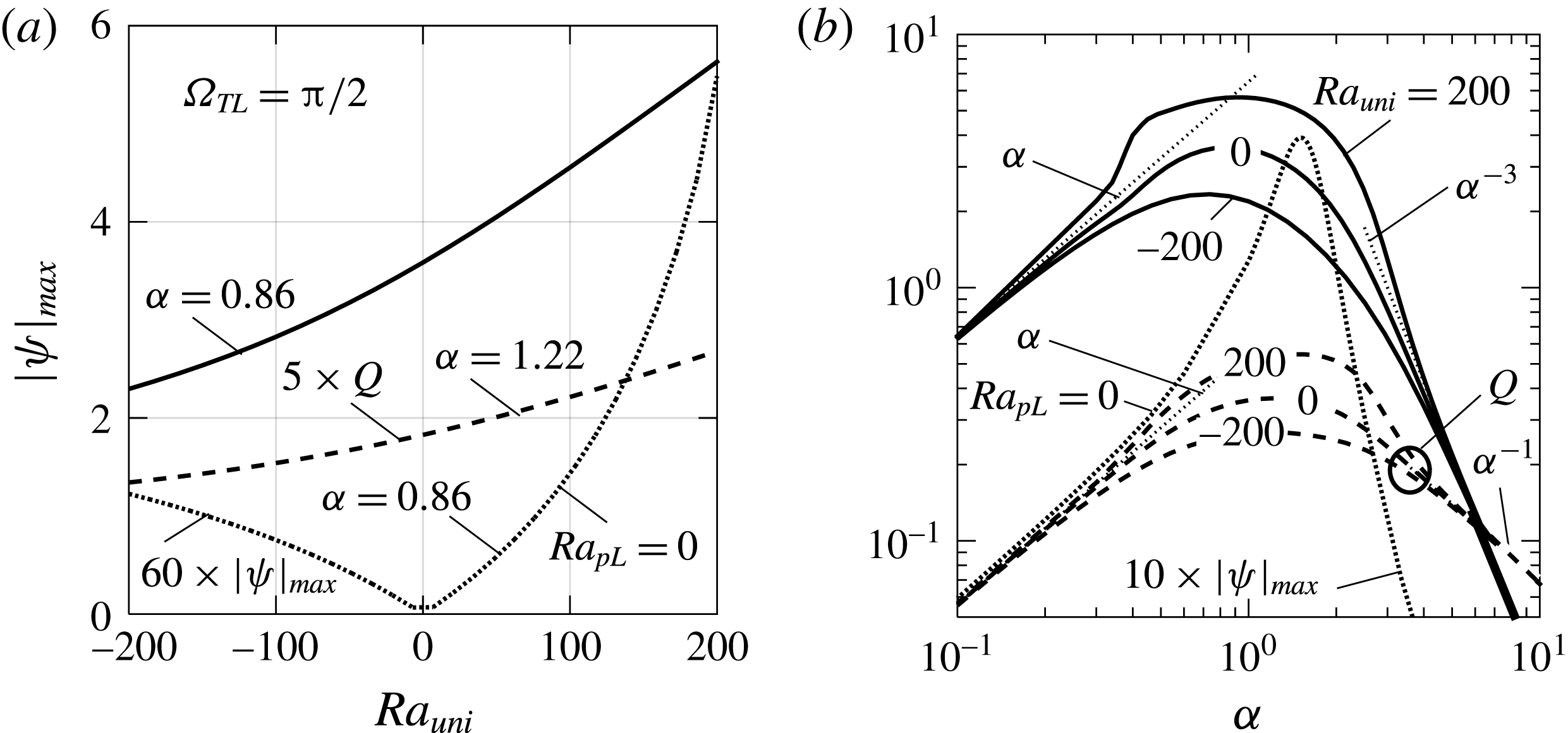
We shall now return the corrugations and the heating to the lower plate and investigate changes associated with introduction of the uniform heating/cooling component. The topology of the flow field is not affected. Increasing $Ra_{uni}$ increases both $|\unicode[STIX]{x1D713}|_{max}$ and $Q$ nearly linearly (see figure 11 a). Cooling of the lower plate, which corresponds to negative values of $Ra_{uni}$ , decrease $|\unicode[STIX]{x1D713}|_{max}$ and $Q$ also almost linearly. 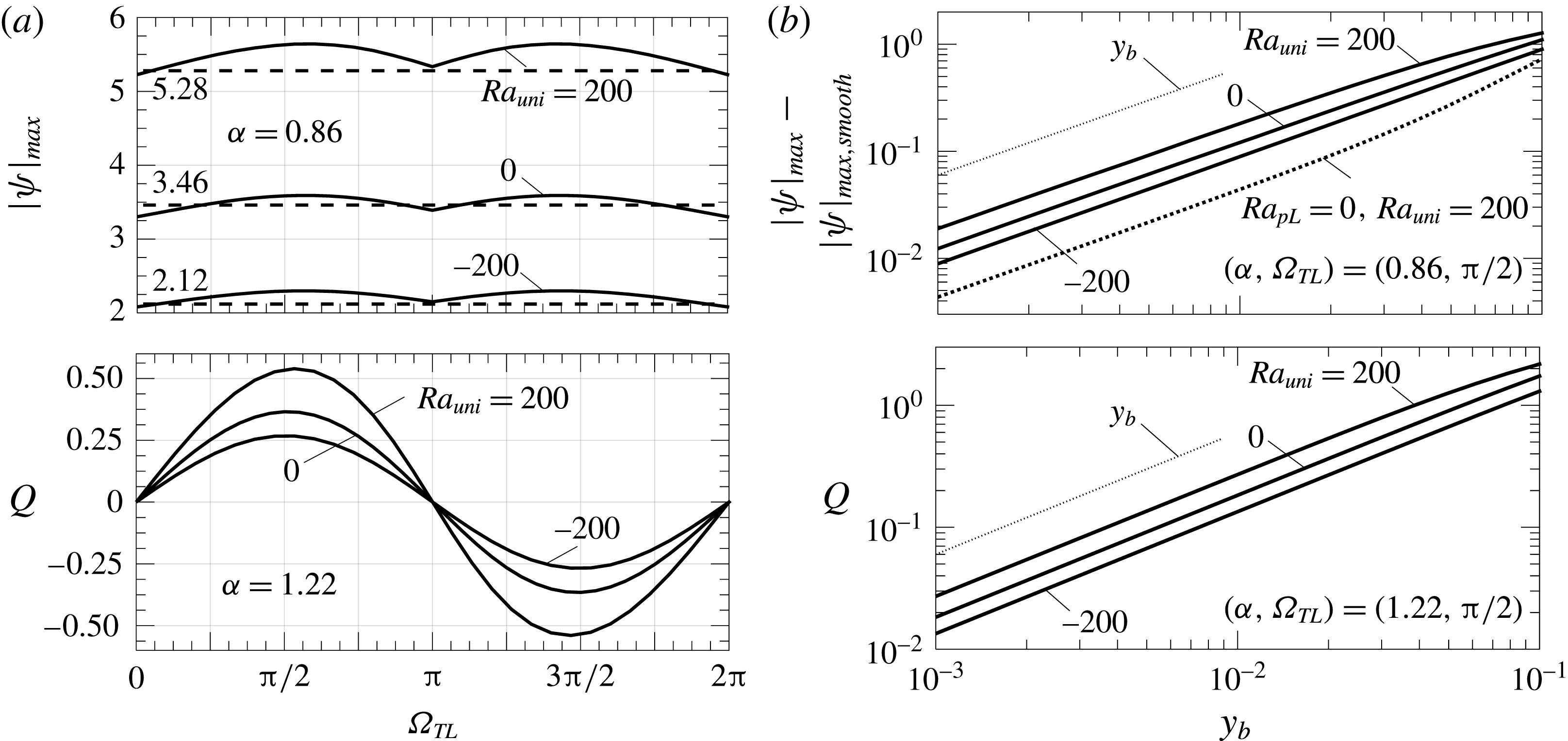The most intense convection occurs for $\unicode[STIX]{x1D6FC}=O(1)$ and it decreases rapidly for $\unicode[STIX]{x1D6FC}\rightarrow 0$ and $\unicode[STIX]{x1D6FC}\rightarrow \infty$ always in the same manner regardless of the value of $Ra_{uni}$ (see figure 11 b). Intensity of convection changes in the same manner as a function of $\unicode[STIX]{x1D6FA}_{TL}$ for all values of $Ra_{uni}$ while the amplitudes of variation of both $|\unicode[STIX]{x1D713}|_{max}$ and $Q$ increase significantly with increasing $Ra_{uni}$ and decrease with negative values of $Ra_{uni}$ (see figure 12 a). Both $|\unicode[STIX]{x1D713}|_{max}$ and $Q$ increase proportionally to $y_{b}$ above the level found in the case of a smooth slot (see figure 12 b).

Figure 11.

Variations of $|\unicode[STIX]{x1D713}|_{max}$ (solid lines), and $Q$ (dashed lines) as functions of $Ra_{uni}$ for $(\unicode[STIX]{x1D6FC},\unicode[STIX]{x1D6FA}_{TL})$ values which maximize them (a) and as functions of $\unicode[STIX]{x1D6FC}$ for $\unicode[STIX]{x1D6FA}_{TL}=\unicode[STIX]{x03C0}/2$ (b). All results are for $y_{b}=0.02,Ra_{pL}=400$ . Dotted lines describe a purely uniform heating ( $Ra_{pL}=0,Ra_{uni}=200$ ). Thin dotted lines identify various asymptotes.

Figure 12.

Variations of $|\unicode[STIX]{x1D713}|_{max}$ and $Q$ as functions of $\unicode[STIX]{x1D6FA}_{TL}$ for $y_{b}=0.02,Ra_{pL}=400$ (a) and as functions of $y_{b}$ for $Ra_{pL}=400$ and $(\unicode[STIX]{x1D6FC},\unicode[STIX]{x1D6FA}_{TL})$ values which maximize them (b). Dashed lines provide data for the smooth slot. Dotted line in figure 13(b) provides data for a purely uniform heating ( $Ra_{pL}=0,Ra_{uni}=200$ ). Thin dotted lines identify various asymptotes. A purely uniform heating with $Ra_{uni}=200$ results in $|\unicode[STIX]{x1D713}|_{max}=0.0914$ .

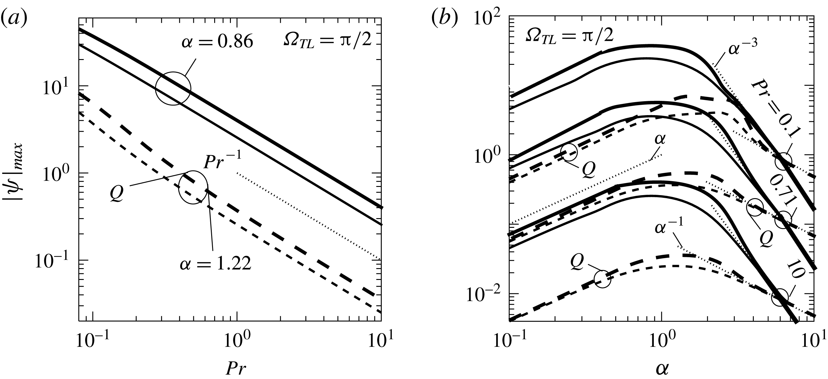
6 Effects of Prandtl number

All results presented in the previous sections have been obtained for $Pr=0.71$ . A decrease of the Prandtl number leads to an increase of the horizontal temperature gradients, which results in an increase of the intensity of convection, i.e. increases of $|\unicode[STIX]{x1D713}|_{max}$ and $Q$ (see figure 13 a). 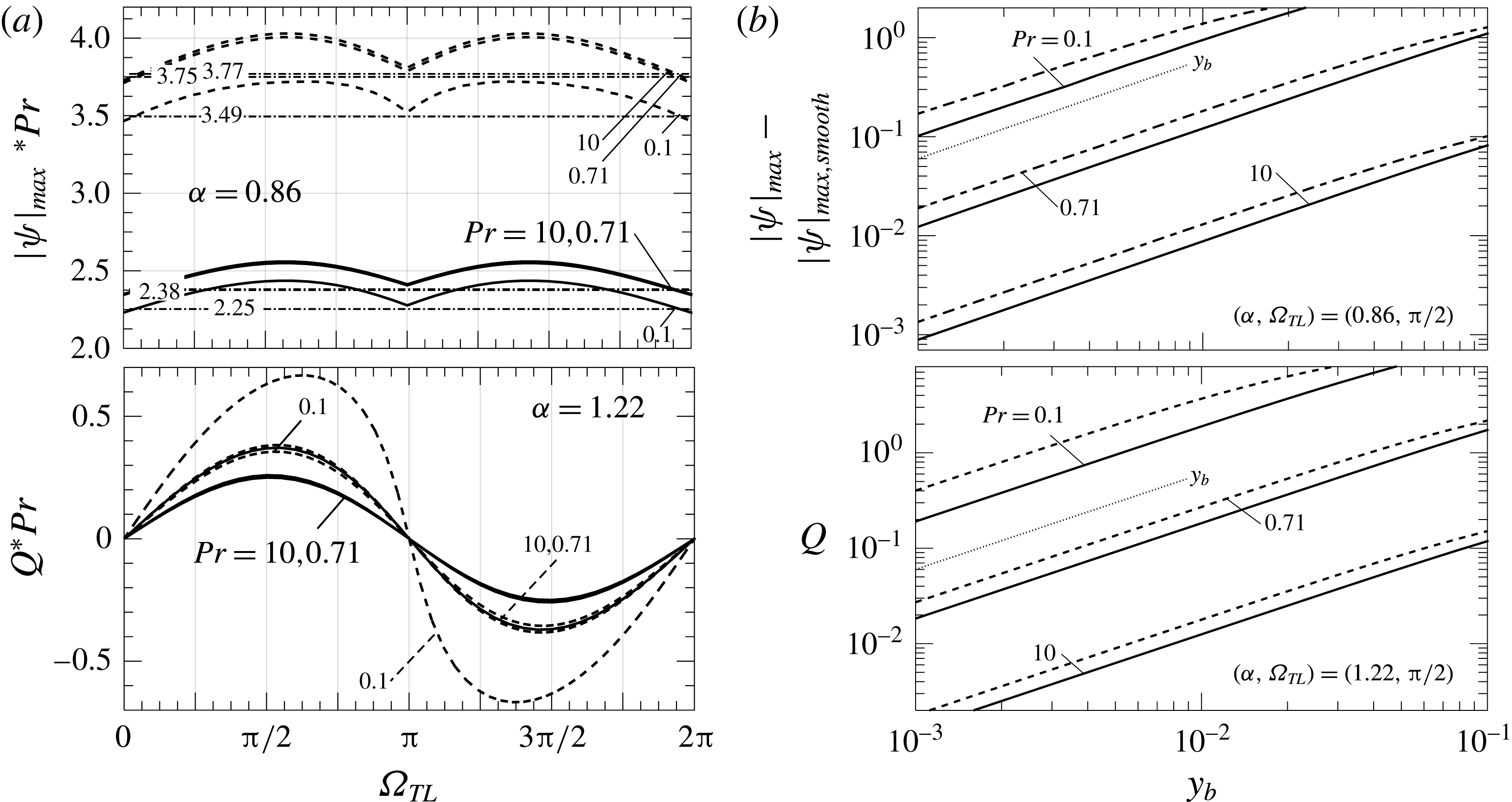The most intense convection occurs for $\unicode[STIX]{x1D6FC}=O(1)$ and decreases rapidly for $\unicode[STIX]{x1D6FC}\rightarrow 0$ and $\unicode[STIX]{x1D6FC}\rightarrow \infty$ in the same manner for all values of $Pr$ (see figure 13 b). Convection intensity changes also in the same manner as a function of $\unicode[STIX]{x1D6FA}_{TL}$ (figure 14 a), while the amplitudes of variation of both $|\unicode[STIX]{x1D713}|_{max}$ and $Q$ increase significantly with a reduction in $Pr$ (figure 14 b).

Figure 13.

Variations of $|\unicode[STIX]{x1D713}|_{max}$ (solid lines), and $Q$ (dashed lines) as functions of $Pr$ for $\unicode[STIX]{x1D6FA}_{TL}=\unicode[STIX]{x03C0}/2$ and $\unicode[STIX]{x1D6FC}$ values which maximize them when $Pr=0.71$ (a) and as functions of $\unicode[STIX]{x1D6FC}$ (b) for $y_{b}=0.02,Ra_{pL}=400$ . Thick and thin solid (dashed) lines correspond to $Ra_{uni}=200$ , 0, respectively. Thin dotted lines identify various asymptotes.

Figure 14.

Variations of $|\unicode[STIX]{x1D713}|_{max}$ , and $Q$ as functions of $\unicode[STIX]{x1D6FA}_{TL}$ for $y_{b}=0.02$ (a) and as functions of $y_{b}$ for $(\unicode[STIX]{x1D6FC},\unicode[STIX]{x1D6FA}_{TL})$ values which maximize them when $Pr=0.71$ (b). In all cases, $Ra_{pL}=400$ , $Ra_{uni}=0$ (solid lines) and $Ra_{uni}=200$ (dashed lines). Dashed–dotted lines provide data for the smooth slot. Thin dotted lines identify various asymptotes.