1 Introduction
Gravity currents are thin, horizontal flows that are driven by the buoyancy difference between an intruding and an ambient fluid, and occur in a wide range of natural and industrial settings (Simpson Reference Simpson1999; Huppert Reference Huppert2006). When gravity currents propagate over a porous substrate, some of the mass in the current can leak into the substrate, slowing down and sometimes inhibiting the propagation of the current. Such flow configurations could occur, for example, when a breaking wave interacts with the sediment on continental shelf (Boczar-Karakiewicz, Bona & Pelchat Reference Boczar-Karakiewicz, Bona and Pelchat1991), during a spill of contaminating liquids from containers surrounded by gravel beds (Grobelbauer, Fannelop & Britter Reference Grobelbauer, Fannelop and Britter1993), following the sequestration of CO
 $_{2}$
in deep aquifers (Huppert & Neufeld Reference Huppert and Neufeld2014), when glacial melt-water reaches the interface between the base of the ice and a porous bed (Das et al.
Reference Das, Joughin, Behn, Howat, King, Lizarralde and Bhatia2008) or when honey spreads over a slice of bread.
Viscous gravity currents on impermeable, flat substrates are known to have self-similar solutions (Huppert Reference Huppert1982), with the fluid front propagating as
 $t^{1/2}$
when the fluid is discharged axisymmetrically at constant rate. Viscous currents on permeable substrates involve two moving fronts, a fluid front that propagates over the substrate, and a drainage front that demarcates the leading position where fluid percolates into the substrate (Thomas, Marino & Linden Reference Thomas, Marino and Linden1998; Pritchard, Woods & Hogg Reference Pritchard, Woods and Hogg2001; Spannuth et al.
Reference Spannuth, Neufeld, Wettlaufer and Worster2009). Where such currents are fed by a constant flux, leakage through the substrate grows as the contact area of the current with the substrate increases until eventually leakage balances the influx allowing the current to reach a steady state (Spannuth et al.
Reference Spannuth, Neufeld, Wettlaufer and Worster2009), in contrast with the case for gravity currents on an impermeable substrate.
The leakage of gravity currents that propagate over saturated porous substrates typically involves a low pore Reynolds number and therefore can be modelled with Darcy’s law. The case of a thin porous substrate may be modelled using only a pressure gradient component acting over the constant thickness of the substrate (Thomas et al. Reference Thomas, Marino and Linden1998; Ungarish & Huppert Reference Ungarish and Huppert2000; Pritchard et al. Reference Pritchard, Woods and Hogg2001; Marino & Thomas Reference Marino and Thomas2002). In the case of deep porous media of both inertial and viscous currents, percolation laws typically account for gravity in addition to a pressure gradient component that is applied over the evolving depth of the draining fluid in the porous medium (Acton, Huppert & Worster Reference Acton, Huppert and Worster2001; Thomas, Marino & Linden Reference Thomas, Marino and Linden2004; Spannuth et al. Reference Spannuth, Neufeld, Wettlaufer and Worster2009).
The position of the fluid and drainage fronts coincide if leakage begins immediately once fluid contacts the substrate. In contrast, the presence of a finite capillary entry pressure can limit the migration of the propagating fluid into the porous substrate, resulting in the fluid and the drainage fronts propagating at different rates. Interfacial tension acting between the invading liquid and the ambient pore fluid restricts the propagating fluid from passing through pore throats (Bear Reference Bear1988). The magnitude of the capillary entry pressure depends on the interfacial tension between the two fluid phases and on the pore size. The presence of a capillary entry pressure requires the fluid in the current to have a minimum overpressure before it can overcome the capillary entry pressure and drain through the surface layer of the substrate.
The impact of capillary pressure on percolation has been previously studied in several contexts. Viscous spreading of a liquid drop on a porous substrate can involve rich and complex structure, and accounting for the movement of contact lines within the pores can become important (Davis & Hocking Reference Davis and Hocking2000, Reference Davis and Hocking1999). In the case of a gravity current propagating within a porous layer along a low-permeability barrier (Woods & Farcas Reference Woods and Farcas2009) the impact of finite capillary entry pressure has led to the partitioning of the current into several regions, including a steady region in which drainage was active, an intermediate region in which the depth of the surface current is equal to the capillary depth and a region in which the propagation of the surface current is similar to a gravity current in a porous layer on impermeable surface (Huppert & Woods Reference Huppert and Woods1995).
In the present study we consider the propagation of an axisymmetric viscous gravity current over a porous substrate with conditional percolation set by a capillary entry pressure. We investigate the evolution of such currents over a relatively thin substrate using theoretical and numerical analysis, combined with laboratory experiments. Specifically, we develop a physical model which accounts for the explicit evolution of the free surface and of the two fronts. In addition, we validate the numerical results with early-time and late-time asymptotic solutions and develop semi-analytical solutions for the evolution of the fronts and the free surface. The results of our theoretical model are tested in the laboratory using an experimentally determined drainage law which phenomenologically captures the behaviour of our theoretical model. The results of the combined theoretical and experimental study are then discussed.
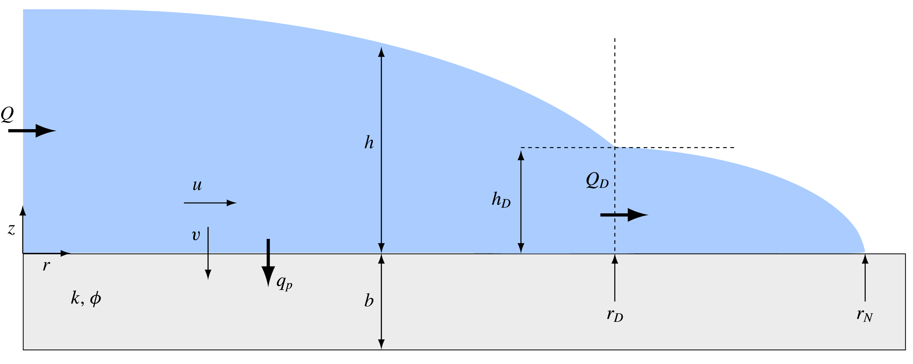
Schematic diagram of a gravity current on a porous substrate with finite entry pressure. The current has a thick inner region (
 $r\leqslant r_{D}(t)$
) in which the drainage through the substrate is
 $q_{p}>0$
and a shallower outer region (
 $r_{D}(t)<r\leqslant r_{N}(t)$
) in which the fluid depth in under the critical capillary depth.

2 Theoretical analysis
2.1 Physical model
We consider a fluid of kinematic viscosity
 ${\it\nu}$
and density
 ${\it\rho}$
that spreads axisymmetrically over a flat, porous substrate of permeability
 $k$
, porosity
 ${\it\phi}$
and thickness
 $b$
(see figure 1). For such long, thin viscous currents, when the leakage rate is small, the pressure within the current is nearly hydrostatic. When the viscous current extends over a distance much greater than the capillary length,
 $$\begin{eqnarray}\displaystyle \ell _{c}=\frac{{\it\gamma}}{{\it\rho}g}, & & \displaystyle\end{eqnarray}$$
where
 ${\it\gamma}$
is the surface tension and
 $g$
the gravitational acceleration, we may neglect capillary forces on the top surface of the current. The upper surface of the current is stress free and, when the porosity and permeability of the substrate are small, we may apply a no-slip condition at the porous interface, to leading order. The radial velocity, driven by gradient in the hydrostatic pressure, is
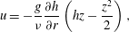 $$\begin{eqnarray}\displaystyle u=-\frac{g}{{\it\nu}}\frac{\partial h}{\partial r}\left(hz-\frac{z^{2}}{2}\right), & & \displaystyle\end{eqnarray}$$
where
 $r,z$
are respectively the radial and vertical coordinates, and
 $h(r,t)$
is the fluid thickness. The horizontal flux, given by the depth-integrated radial velocity, is
 $$\begin{eqnarray}\displaystyle q=\int _{0}^{h}u\,\text{d}z=-\frac{g}{3{\it\nu}}h^{3}\frac{\partial h}{\partial r}. & & \displaystyle\end{eqnarray}$$
Local conservation of mass implies that
 $$\begin{eqnarray}\displaystyle \frac{\partial h}{\partial t}+\frac{1}{r}\frac{\partial }{\partial r}(rq)=-v_{p}, & & \displaystyle\end{eqnarray}$$
where
 $v_{p}$
is the vertical leakage flux due to drainage through the porous substrate.
When the substrate is initially dry, capillary forces acting on the small length scale of the pore diameter
 $d_{p}$
act to inhibit entry of the fluid into the substrate. To initiate the flow
 $v_{p}$
in the substrate, the fluid pressure must exceed the capillary entry pressure. The fluid pressure is predominately hydrostatic when the length of the surface current is much larger than its depth, and hence the fluid must reach a critical depth to initiate drainage, which we denote as the capillary depth
 $h_{D}$
(Bear Reference Bear1988). The leakage flow is then driven by the overpressure of the fluid above the substrate. Where the depth of the propagating fluid is less than the capillary depth, interfacial tension inhibits flow into the substrate. The control on drainage exerted by the capillary entry pressure results in a discontinuous boundary condition on the dynamics of the propagating current,
 $$\begin{eqnarray}\displaystyle v_{p}=\left\{\begin{array}{@{}ll@{}}\displaystyle {\it\phi}\frac{kg}{{\it\nu}}\left(\frac{h}{b}+1\right), & h\geqslant h_{D},\\ \displaystyle 0, & h<h_{D},\end{array}\right. & & \displaystyle\end{eqnarray}$$
where
 $$\begin{eqnarray}\displaystyle h_{D}=\frac{4{\it\gamma}\cos {\it\theta}}{{\it\rho}gd_{p}} & & \displaystyle\end{eqnarray}$$
is the critical depth of the surface current corresponding to the critical capillary entry pressure, with contact angle
 ${\it\theta}$
. Here we have modelled the percolation velocity using Darcy’s law, with fluid flow being driven by both the pressure gradient across the substrate and the weight of the fluid. This expression for the leakage is valid once the fluid fills the entire depth of the porous layer, namely, on time scales longer than
 $b/v_{p}$
. For thin substrates, the time scale for the viscous propagation of the fluid front through the substrate is shorter; and so we neglect to model the evolving fluid front within the porous layer, as has been done previously for deep porous media (e.g. Davis & Hocking Reference Davis and Hocking2000; Spannuth et al.
Reference Spannuth, Neufeld, Wettlaufer and Worster2009). Substituting (2.3), (2.5) in (2.4), the evolution of the axisymmetric current may be described by
 $$\begin{eqnarray}\displaystyle \frac{\partial h}{\partial t}-\frac{g}{3{\it\nu}}\frac{1}{r}\frac{\partial }{\partial r}\left(rh^{3}\frac{\partial h}{\partial r}\right)=\left\{\begin{array}{@{}ll@{}}\displaystyle -{\it\phi}\frac{kg}{{\it\nu}}\left(\frac{h}{b}+1\right), & r<r_{D},\\ \displaystyle 0, & r_{D}\leqslant r\leqslant r_{N},\end{array}\right. & & \displaystyle\end{eqnarray}$$
where the drainage front
 $r=r_{D}(t)$
continuously adjusts to satisfy the condition that
 $h(r_{D},t)=h_{D}$
and
 $r=r_{N}(t)$
is the fluid front where
 $h(r_{N},t)=0$
. The four boundary conditions necessary to fully specify the problem are
 $$\begin{eqnarray}\displaystyle & \displaystyle 2{\rm\pi}rq=Q\quad \text{as }r\rightarrow 0, & \displaystyle\end{eqnarray}$$
 $$\begin{eqnarray}\displaystyle & \displaystyle h=h_{D}\quad \text{at }r=r_{D}, & \displaystyle\end{eqnarray}$$
 $$\begin{eqnarray}\displaystyle & \displaystyle 2{\rm\pi}rq=0\quad \text{at }r=r_{N}, & \displaystyle\end{eqnarray}$$
 $$\begin{eqnarray}\displaystyle & \displaystyle h=0\quad \text{at }r=r_{N}. & \displaystyle\end{eqnarray}$$
These conditions specify the input flux
 $Q$
at the origin, the critical depth set by the capillary entry pressure at the edge of the drainage region and conditions of zero flux through and zero height at the nose of the current, respectively. The boundary condition (2.7d
) can be derived from a statement of global mass conservation
 $$\begin{eqnarray}\displaystyle 2{\rm\pi}\int _{0}^{r_{N}}rh\,\text{d}r+2{\rm\pi}\int _{0}^{r_{D}}\int _{0}^{t}v_{p}r\,\text{d}t\,\text{d}r=Qt, & & \displaystyle\end{eqnarray}$$
by differentiating (2.8) with respect to time, and using (2.7). We note that continuity of both
 $h$
and the local flux
 $q\propto \partial h/\partial r$
at
 $r=r_{D}$
is implicit in (2.7).
2.2 Dimensionless quantities
Unlike the flow of viscous fluids over an impermeable surface, a unique vertical length scale exists in the problem due to the capillary forces acting within the pore space as represented by the critical depth. We therefore non-dimensionalise (2.7) by scaling depth by the drainage height, the radial extent by the steady-state balance between horizontal flux and leakage and time by the characteristic time to reach the steady state,
 $$\begin{eqnarray}\displaystyle {\hat{h}}=h/h_{D},\quad \hat{r}=r\left/\sqrt{\frac{h_{D}^{4}}{3{\it\phi}k}}\right.,\quad \hat{t}=t\left/\left(\frac{{\it\nu}h_{D}}{{\it\phi}kg}\right)\right.. & & \displaystyle\end{eqnarray}$$
Therefore, the dimensionless equations (hats removed) are
 $$\begin{eqnarray}\displaystyle \frac{\partial h}{\partial t}-\frac{1}{r}\frac{\partial }{\partial r}\left(rh^{3}\frac{\partial h}{\partial r}\right)=\left\{\begin{array}{@{}ll@{}}\displaystyle -({\it\lambda}h+1), & r<r_{D},\\ \displaystyle 0, & r_{D}\leqslant r\leqslant r_{N},\end{array}\right. & & \displaystyle\end{eqnarray}$$
with the boundary conditions,
 $$\begin{eqnarray}\displaystyle & \displaystyle rh^{3}\frac{\partial h}{\partial r}=-\mathscr{Q}\quad \text{as }r\rightarrow 0, & \displaystyle\end{eqnarray}$$
 $$\begin{eqnarray}\displaystyle & \displaystyle h=1\quad \text{at }r=r_{D}, & \displaystyle\end{eqnarray}$$
 $$\begin{eqnarray}\displaystyle & \displaystyle rh^{3}\frac{\partial h}{\partial r}=0\quad \text{at }r=r_{N}, & \displaystyle\end{eqnarray}$$
 $$\begin{eqnarray}\displaystyle & \displaystyle h=0\quad \text{at }r=r_{N}, & \displaystyle\end{eqnarray}$$
where the system is now a function of two non-dimensional quantities,
 $$\begin{eqnarray}\displaystyle {\it\lambda}=\frac{h_{D}}{b},\quad \mathscr{Q}=\frac{3{\it\nu}Q}{2{\rm\pi}gh_{D}^{4}}, & & \displaystyle\end{eqnarray}$$
that characterise the critical entry depth and the input flux respectively.
2.3 Numerical solution of the full evolution
The full temporal evolution of the flow is found numerically by integrating (2.10), which we do by mapping the percolating and non-percolating domains on to a fixed interval. Such mappings involve two additional evolution equations for the fronts
 $$\begin{eqnarray}\displaystyle & \displaystyle {\dot{r}}_{D}=-\left.\frac{\partial h/\partial t}{\partial h/\partial r}\right|_{r=r_{D}}, & \displaystyle\end{eqnarray}$$
 $$\begin{eqnarray}\displaystyle & \displaystyle {\dot{r}}_{N}=\left.\frac{q}{h}\right|_{r=r_{N}}, & \displaystyle\end{eqnarray}$$
 $$\begin{eqnarray}\displaystyle \unicode[STIX]{x27E6}h\unicode[STIX]{x27E7}=\unicode[STIX]{x27E6}q\unicode[STIX]{x27E7}=0\quad \text{at }r=r_{D}, & & \displaystyle\end{eqnarray}$$
which correspond to continuity of thickness and flux at the interface. We solve the complete system simultaneously for the free surface and the position of the front in each domain (appendix A). We evaluate the quality of our numerical scheme by checking consistency of the case of no drainage with the self-similar solution of a gravity current on an impermeable substrate (Huppert Reference Huppert1982), which we also use as an initial condition. We have also confirmed consistency of the numerical solution with the analytical solutions of the fully prewetted substrate (appendix A) and of the late-time asymptotic flow in the permeable region (figure 2 a).
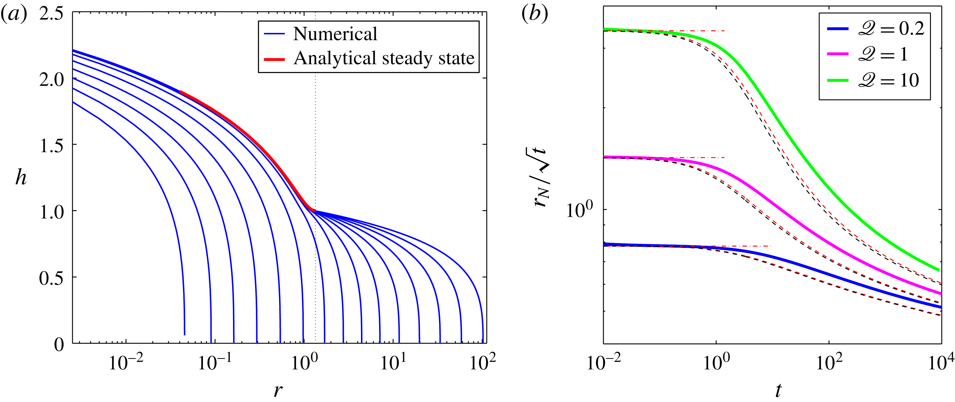
(a) Numerical solution of the evolution of the current for
 ${\it\lambda}=0.1,\mathscr{Q}=1$
, showing the evolution of the free surface (—— blue) starting at
 $t=10^{-2}$
and ending at
 $t=3.8\times 10^{4}$
. The temporal spreading of the profiles is uniform in the
 $\log (t)$
space. The steady-state solution of the drainage-active region in the limit
 $\mathscr{Q}_{D}=0$
(2.17) is shown (—— red), where the position of the steady-state drainage front is marked by a vertical grid line. (b) Evolution of the fluid front
 $r_{N}$
for
 ${\it\lambda}=0.1$
and for
 $\mathscr{Q}=0.2,1,10$
, showing the full numerical solutions (thick curves), the asymptotic estimates of the early time evolution (– - – -, red), and the asymptotic estimates of the late-time evolution (– – – – red) for the case
 ${\it\lambda}\ll 1$
and
 $\mathscr{Q}=0$
and (– – – – black) for the finite
 ${\it\lambda}$
and non-zero
 $\mathscr{Q}_{D}$
case, which are evaluated also at early time.
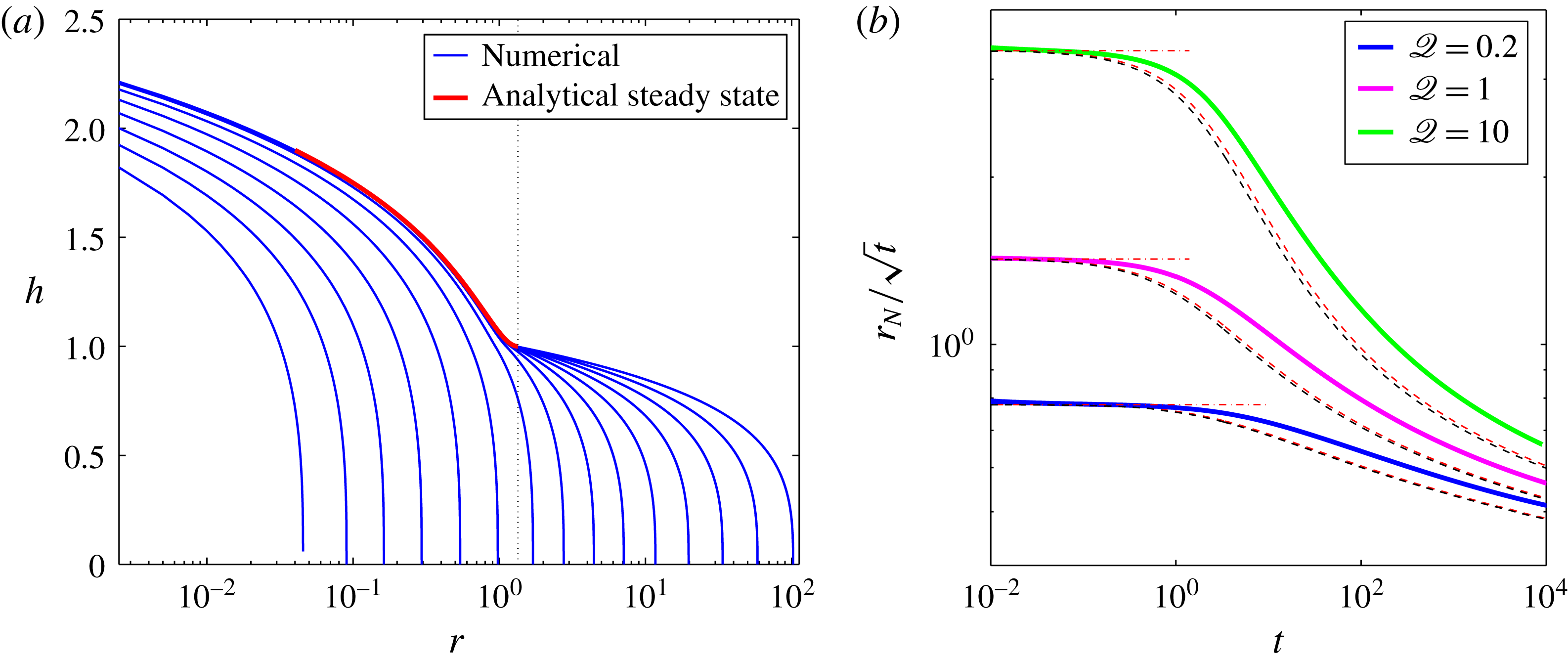
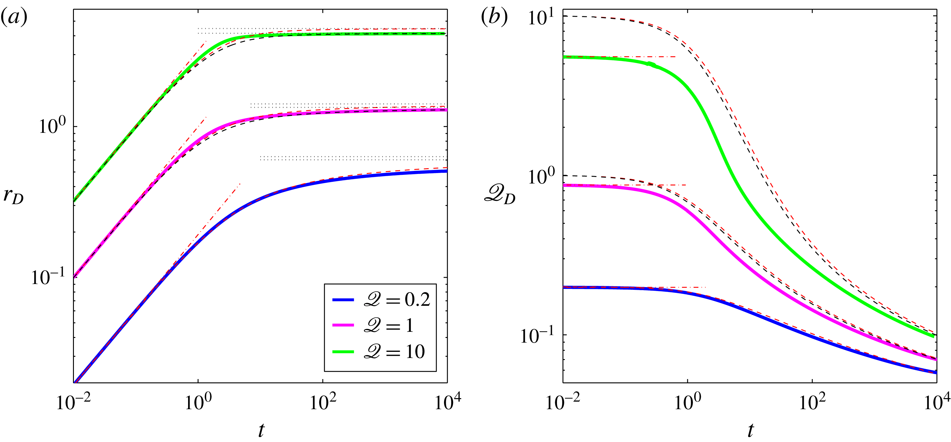
The simulated evolution of the current is shown in figure 2. At early times (
 $t\ll 1$
) drainage is confined to a small region (
 $r_{D}\ll 1$
) and the horizontal flux across the drainage front
 $\mathscr{Q}_{D}$
is roughly equivalent to
 $\mathscr{Q}$
. Therefore the impact of the drainage on the current is negligible and the behaviour is, to leading order, that of a constant flux, viscous gravity current on an impermeable substrate (Huppert Reference Huppert1982), for which
 $r_{N}\sim r_{D}\sim t^{1/2}$
(figures 2
b, 3
a). When
 $t\gg 1$
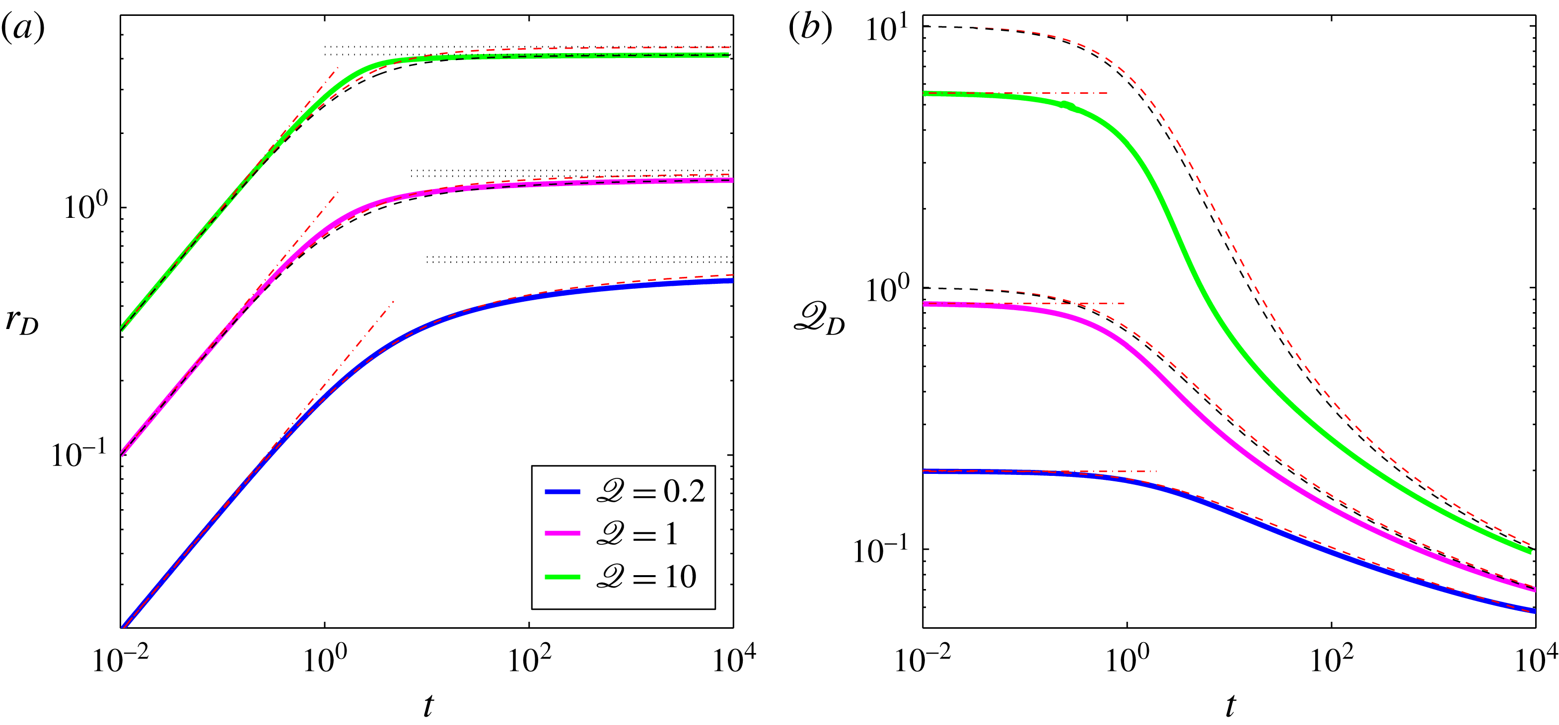
the drainage front slows down and approaches a steady position in which the leakage flux nearly balances the input flux (figure 3
a), while the fluid front advances again as
 $t^{1/2}$
, albeit with a smaller prefactor that varies slowly in time, equivalent to a reduced input flux (figure 2
b). In this regime, the flux across the drainage front becomes smaller than
 $Q$
and decreases indefinitely (figure 3
b). To obtain a more quantitative evaluation of the quality of the numerical simulation we investigate the asymptotic behaviour of the solutions in the following sections.
(a) Evolution of the drainage front
 $r_{D}$
and (b) the evolution of the horizontal flux at the drainage front
 $\mathscr{Q}_{D}$
for
 ${\it\lambda}=0.1$
and for
 $\mathscr{Q}=0.2,1,10$
, showing the full numerical solutions (thick curves), the asymptotic estimate of the early time evolution (– - – -), the asymptotic estimates of the late-time evolution for
 ${\it\lambda}\ll 1$
,
 $\mathscr{Q}_{D}=0$
(– – – – red) and for the finite
 ${\it\lambda}$
and non-zero
 $\mathscr{Q}_{D}$
case (– – – – black). For each of the three
 $\mathscr{Q}$
values in (a), two horizontal grid lines mark the two approximations of steady-state solutions to equations (2.16), the top being (2.17b
).
2.4 Early-time evolution
At early times (
 $r_{N}\ll 1$
) the drainage front is small,
 $r_{D}\ll 1$
, so that little fluid leaks from the current. In this limit we recover, to leading order, the self-similar spreading of an non-leaking current (Huppert Reference Huppert1982), in which the viscous gravity current has a self-similar form for the height and radial extent given by
 $$\begin{eqnarray}\displaystyle & \displaystyle h(r,t)={\it\xi}_{N}^{2/3}(2{\rm\pi}\mathscr{Q})^{1/4}{\it\psi}(y), & \displaystyle\end{eqnarray}$$
 $$\begin{eqnarray}\displaystyle & \displaystyle r_{N}={\it\xi}_{N}(2{\rm\pi}\mathscr{Q})^{3/8}t^{1/2}, & \displaystyle\end{eqnarray}$$
 ${\it\xi}=r(2{\rm\pi}\mathscr{Q})^{-3/8}t^{-1/2}$
,
 $y={\it\xi}/{\it\xi}_{N}$
and
 ${\it\xi}_{N}={\it\xi}(r=r_{N})\approx 0.715$
together with
 ${\it\psi}(z)$
describe the self-similar solution in the absence of leakage (Huppert Reference Huppert1982). The position of the drainage front is given by
 $$\begin{eqnarray}\displaystyle r_{D}=y_{D}r_{N}, & & \displaystyle\end{eqnarray}$$
where
 $y=y_{D}$
is defined by the relationship
 $$\begin{eqnarray}\displaystyle h(r_{D},t)=1={\it\xi}_{N}^{2/3}(2{\rm\pi}\mathscr{Q})^{1/4}{\it\psi}(y_{D}) & & \displaystyle\end{eqnarray}$$
and approaches to 1 asymptotically with
 $\mathscr{Q}$
, implying that at early times the larger
 $\mathscr{Q}$
is, the closer
 $r_{D}$
is to
 $r_{N}$
. The corresponding flux at the drainage front
 $$\begin{eqnarray}\displaystyle \mathscr{Q}_{D}\equiv -r_{D}\left.\frac{\partial h}{\partial r}\right|_{r_{D}}=-y_{D}{\it\xi}_{N}^{2/3}(2{\rm\pi}\mathscr{Q})^{1/4}\left.\frac{\partial {\it\psi}}{\partial y}\right|_{y_{D}} & & \displaystyle\end{eqnarray}$$
is constant.
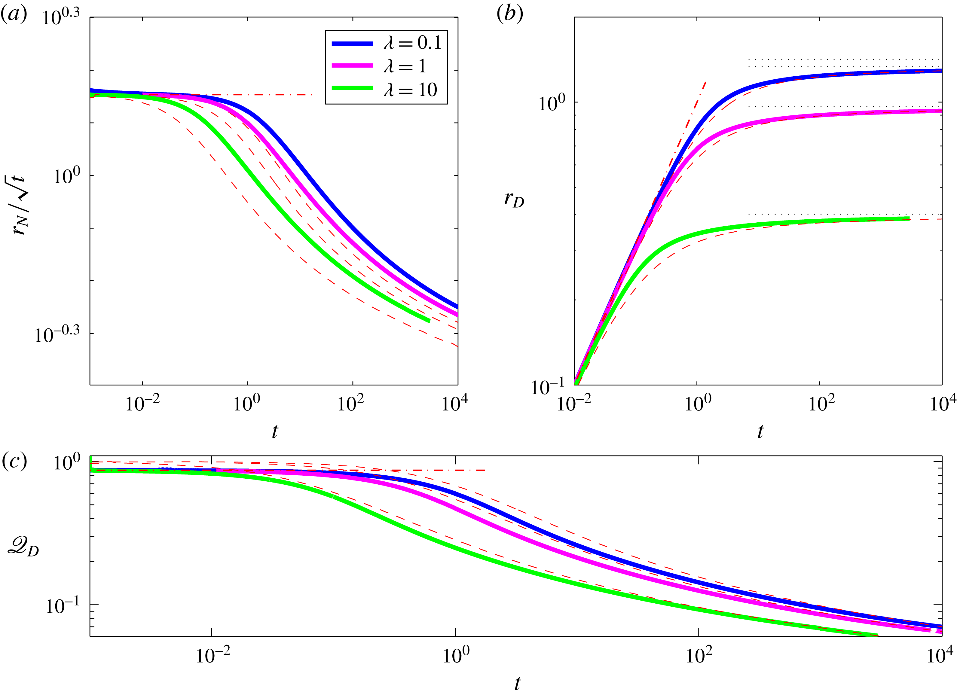
We use the solution (2.14) to initialize our numerical solutions and confirm that the predicted asymptotic structure is preserved at early times. In particular we find that the early time behaviour of the fluid and drainage fronts and of the flux at the drainage front follow the predictions in (2.14b
), (2.15a
), (2.15c
) independently of the value of
 $\mathscr{Q}$
(figures 2
b, 3) and independently of the value of
 ${\it\lambda}$
(figure 4).
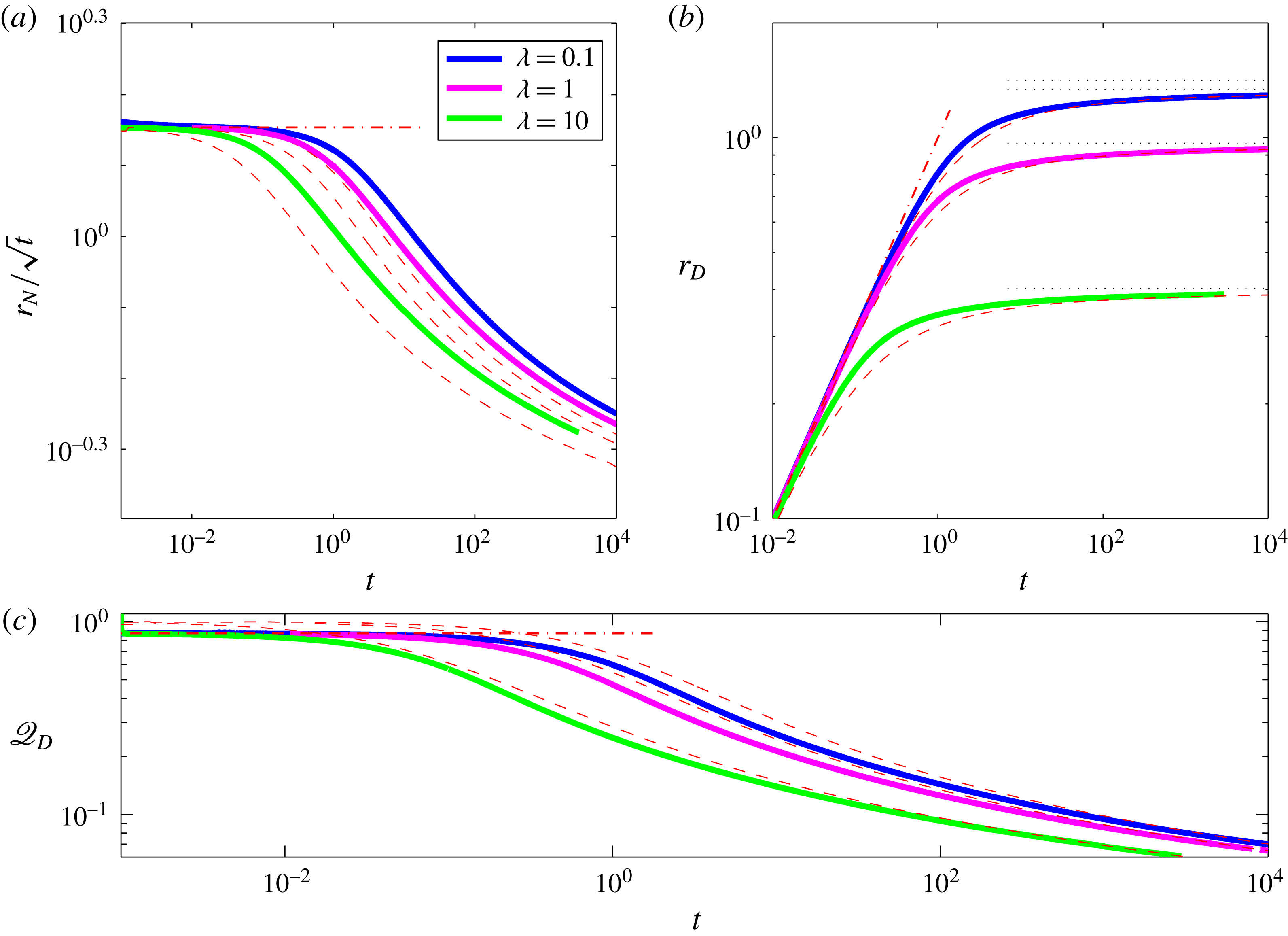
Evolution of the fluid front
 $r_{N}$
(a), the drainage front
 $r_{D}$
(b) and the horizontal flux at the drainage front
 $\mathscr{Q}_{D}$
(c) for
 $\mathscr{Q}=1$
and for
 ${\it\lambda}=0.1,1,10$
, showing the full numerical solutions (thick curves), and the asymptotic estimate of the early time evolution (– -) and of the late-time evolution (– – – –).
2.5 Late-time evolution
2.5.1 The draining domain
As the radius of the current expands, the extent of the drainage front increases and the drainage flux becomes comparable to the input flux. In this limit we may anticipate an interior steady state in which leakage balances the input flux to leading order. We therefore look for steady solutions of (2.10a ),
 $$\begin{eqnarray}\displaystyle \frac{1}{r}\frac{\text{d}}{\text{d}r}\left(rh^{3}\frac{\text{d}h}{\text{d}r}\right)={\it\lambda}h+1\quad \text{for }r\leqslant r_{D}, & & \displaystyle\end{eqnarray}$$
subject to the imposed input flux at the origin, the height of the current equal to the critical drainage height at
 $r_{D}$
and to a limiting flux
 $\mathscr{Q}_{D}$
to the outer current,
 $$\begin{eqnarray}\displaystyle & \displaystyle -rh^{3}\frac{\text{d}h}{\text{d}r}=\mathscr{Q}\quad \text{as }r\rightarrow 0, & \displaystyle\end{eqnarray}$$
 $$\begin{eqnarray}\displaystyle & \displaystyle h=1\quad \text{at }r=r_{D}, & \displaystyle\end{eqnarray}$$
 $$\begin{eqnarray}\displaystyle & \displaystyle -r_{D}\frac{\text{d}h}{\text{d}r}=\mathscr{Q}_{D}\quad \text{at }r=r_{D}. & \displaystyle\end{eqnarray}$$
In the limit
 ${\it\lambda}\ll 1$
we find the closed-form solution
 $$\begin{eqnarray}\displaystyle & \displaystyle h=[1+r^{2}-r_{D}^{2}-4\mathscr{Q}\ln (r/r_{D})]^{1/4}, & \displaystyle\end{eqnarray}$$
 $$\begin{eqnarray}\displaystyle & \displaystyle r_{D}=\sqrt{2(\mathscr{Q}-\mathscr{ Q}_{D})}, & \displaystyle\end{eqnarray}$$
 $h(r_{D}=r_{N})=0$
in that previous work. This difference introduces a fundamentally different long-time behaviour, in which the fluid front in the present study propagates indefinitely.
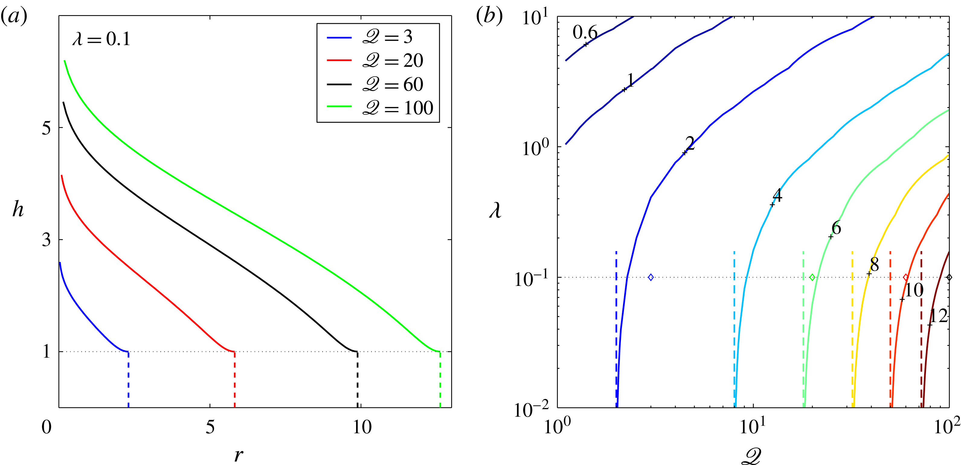
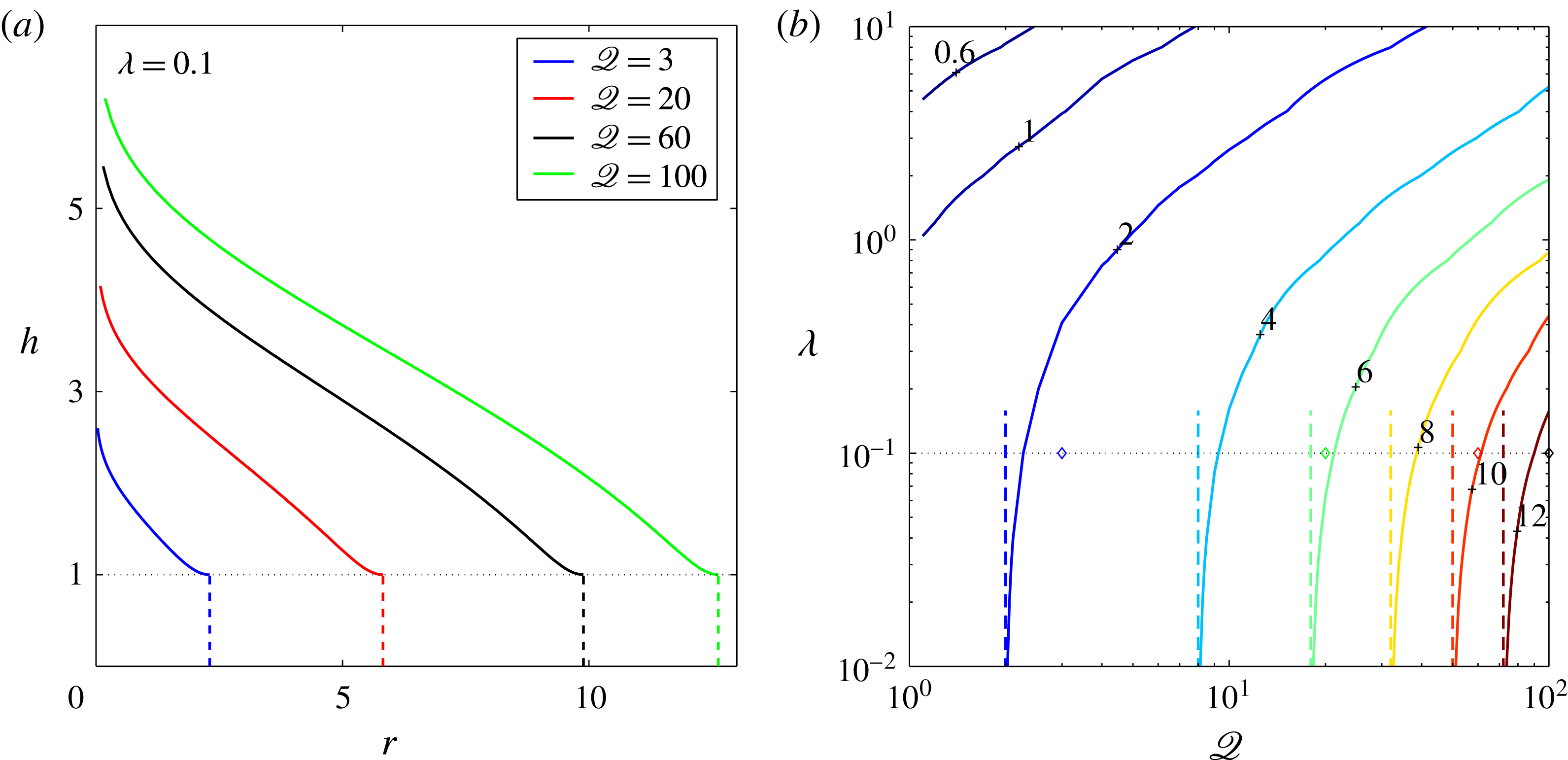
Numerical solutions to the steady-state boundary-value problem in the draining region (2.16). (a) Steady-state solutions of the free surface for
 ${\it\lambda}=0.1$
and for
 $\mathscr{Q}=3,20,60,100$
, where dash lines mark the position of the drainage front in each case. (b) Contours of the steady-state position of the drainage front
 $r_{D}$
as a function of
 $\mathscr{Q}$
and
 ${\it\lambda}$
(solid curves, contour value marked by adjacent numbers). In the limit
 ${\it\lambda}\ll 1$
the solution approaches
 $r_{D}=\sqrt{2\mathscr{Q}}$
(vertical dash lines). The
 $\diamond$
shapes along the
 ${\it\lambda}=0.1$
grid line represent the points in the phase space that correspond to the solutions shown in (a). In all cases we assume that
 $\mathscr{Q}_{D}=0$
.
The steady-state system (2.16) is second order in
 $h$
and involves two unknowns (
 $r_{D}$
and
 $\mathscr{Q}_{D}$
), therefore four boundary conditions are required to solve it. The fourth relation can be provided by the solution to the outer current (§ 2.5.2), which leads to a full late-time solution (see § 2.5.3). Despite the missing information at this stage, reasonable progress can be made by assuming that at late time
 $\mathscr{Q}_{D}\ll \mathscr{Q}$
, which results in the drainage front
 $r_{D}\approx \sqrt{2\mathscr{Q}}$
for non-dimensional critical thickness
 ${\it\lambda}\ll 1$
. For general
 ${\it\lambda}$
, equations (2.16a
)–(2.16d
) must be solved numerically (here with Matlab’s bvp4c routine). For the numerical solution we substitute the boundary condition (2.16b
) with the time derivative of the integral mass-balance relation (2.8)
 $$\begin{eqnarray}\displaystyle 2{\rm\pi}\int _{0}^{r_{D}}v_{p}r\,\text{d}r=\mathscr{Q}-\mathscr{Q}_{D}, & & \displaystyle\end{eqnarray}$$
where
 $\mathscr{Q}_{D}=0$
and we use the analytic solution (2.17) in the limit
 ${\it\lambda}\rightarrow 0$
to verify the numerical solution. The results indicate that
 $r_{D}$
increases with
 $\mathscr{Q}$
for any given
 ${\it\lambda}$
, decreases with the increase of
 ${\it\lambda}$
for any given
 $\mathscr{Q}$
and converges to the analytical solution (2.17b
) in the limit
 ${\it\lambda}\ll 1$
(see figure 5). These steady-state solutions successfully predict the leading-order solution of the full equations under the assumption of zero flux at the drainage front (e.g. figure 2
a).
2.5.2 The non-draining domain
The approach of the drainage front
 $r_{D}$
to a steady position over time introduces an additional radial length scale, which at first suggests that the evolution of the non-draining part of the current can no longer be self similar. However, after sufficient time
 $r_{D}\ll r_{N}-r_{D}$
and to leading order the position of the drainage front can be approximated as
 $r_{D}\approx 0$
. In this limit, the radial length scale is effectively removed and we may anticipate that the flux
 $\mathscr{Q}_{D}$
past the drainage front is a slowly varying function of time, and that a similarity solution is indeed valid.
To investigate this asymptotic limit, we approximate the solution at the drainage front by matching the asymptotic solutions for the draining and non-draining currents at
 $r_{D}$
. We first consider the propagation of the non-draining current for
 $r_{D}<r<r_{N}$
, described by
 $$\begin{eqnarray}\displaystyle \frac{\partial h}{\partial t}-\frac{1}{r}\frac{\partial }{\partial r}\left(rh^{3}\frac{\partial h}{\partial r}\right)=0, & & \displaystyle\end{eqnarray}$$
with the boundary conditions
 $$\begin{eqnarray}\displaystyle & \displaystyle -rh^{3}\frac{\partial h}{\partial r}=\mathscr{Q}_{D}\quad \text{as }r\rightarrow r_{D}\approx 0, & \displaystyle\end{eqnarray}$$
 $$\begin{eqnarray}\displaystyle & \displaystyle h=1\quad \text{as }r\rightarrow r_{D}\approx 0. & \displaystyle\end{eqnarray}$$
The full numerical solution (§ 2.3) indicates that the approach to the steady state is slow, as the drop of the flux
 $\mathscr{Q}_{D}$
in time is approximately logarithmic, and that
 $r_{N}$
grows nearly like
 $t^{1/2}$
. This leads to the ansatz that the solution to (2.19) may be approximated by the similarity solution for a gravity current on an impermeable surface (2.14). Therefore, we let
 $\mathscr{Q}_{D}=\mathscr{Q}_{D}(s)$
and
 $h(r,t)={\it\zeta}_{N}^{2/3}(2{\rm\pi}\mathscr{Q}_{D}(s))^{1/4}f(x,s)$
, where
 $s\equiv 1/\ln (t)$
,
 $x={\it\zeta}/{\it\zeta}_{N}$
and where
 ${\it\zeta}=r(2{\rm\pi}\mathscr{Q}_{D}(s))^{-3/8}t^{-1/2}$
is a similarity coordinate with
 ${\it\zeta}_{N}\equiv {\it\zeta}(r=r_{N})$
. Substituting these into (2.19) we find
 $$\begin{eqnarray}\displaystyle \frac{x}{2}\frac{\partial f}{\partial x}+\frac{1}{x}\frac{\partial }{\partial x}\left(xf^{3}\frac{\partial f}{\partial x}\right)=\frac{s^{2}}{\mathscr{Q}_{D}}\left(\frac{3}{8}x\frac{\partial f}{\partial x}-\frac{f}{2{\it\zeta}_{N}^{2/3}}\frac{\partial \mathscr{Q}_{D}}{\partial s}\right), & & \displaystyle\end{eqnarray}$$
together with the boundary conditions
 $$\begin{eqnarray}\displaystyle & \displaystyle -2{\rm\pi}{\it\zeta}_{N}^{8/3}xf^{3}\frac{\partial f}{\partial x}=1\quad \text{as }x\rightarrow 0, & \displaystyle\end{eqnarray}$$
 $$\begin{eqnarray}\displaystyle & \displaystyle (2{\rm\pi}\mathscr{Q}_{D})^{1/4}{\it\zeta}_{N}^{2/3}f=1\quad \text{as }x\rightarrow 0. & \displaystyle\end{eqnarray}$$
A scaling analysis of (2.20a
) shows that the right-hand side is
 $O(s^{2}f/\mathscr{Q}_{D},sf)$
, while the left-hand side terms are
 $O(f)$
and
 $O(f^{4}/x^{2})$
. Therefore, as
 $t\rightarrow \infty$
(
 $s\rightarrow 0$
) the dominant balance is independent of
 $s$
and represented by the left-hand side of (2.20a
), which has a similarity solution
 $f={\it\psi}$
identical to (2.14) with a slowly time-dependent flux
 $\mathscr{Q}_{D}(s)$
. Combining the similarity solution for
 $r_{N}$
together with the boundary condition (2.20c
) we find
 $$\begin{eqnarray}\displaystyle & \displaystyle 1={\it\zeta}_{N}^{2/3}(2{\rm\pi}\mathscr{Q}_{D})^{1/4}{\it\psi}(x_{D}), & \displaystyle\end{eqnarray}$$
 $$\begin{eqnarray}\displaystyle & \displaystyle x_{D}=\frac{r_{D}t^{-1/2}}{{\it\zeta}_{N}(2{\rm\pi}\mathscr{Q}_{D})^{3/8}}, & \displaystyle\end{eqnarray}$$
 $x_{D}\equiv r_{D}/r_{N}$
and
 ${\it\zeta}_{N}={\it\xi}_{N}$
, which represents the relation between
 $r_{D}$
and
 $\mathscr{Q}_{D}$
for the outer-spreading current.
Analytic approximated expressions may be found for (2.21) by noting that in the limit
 $x\rightarrow 0$
,
 $f\sim (-\ln x)^{1/4}$
. Hence, in this limit (for
 $x_{D}\rightarrow 0$
) the inner limit of the outer-spreading current may be approximated as
 $$\begin{eqnarray}\displaystyle h(r,t)=\left(-4\mathscr{Q}_{D}\ln \frac{rt^{-1/2}}{{\it\zeta}_{N}(2{\rm\pi}\mathscr{Q}_{D})^{3/8}}\right)^{1/4}, & & \displaystyle\end{eqnarray}$$
which at the drainage front implies (using (2.19c )) that
 $$\begin{eqnarray}\displaystyle 1=-4\mathscr{Q}_{D}\ln x_{D}. & & \displaystyle\end{eqnarray}$$
2.5.3 Asymptotic matching
To determine the late-time behaviour of the current we estimate the position
 $r_{D}$
and flux
 $\mathscr{Q}_{D}$
at the drainage front by matching the asymptotic solution at the draining domain, given by the numerical solution to (2.16) and (2.18), with that at the non-draining domain represented by (2.21) or by the approximation (2.23).
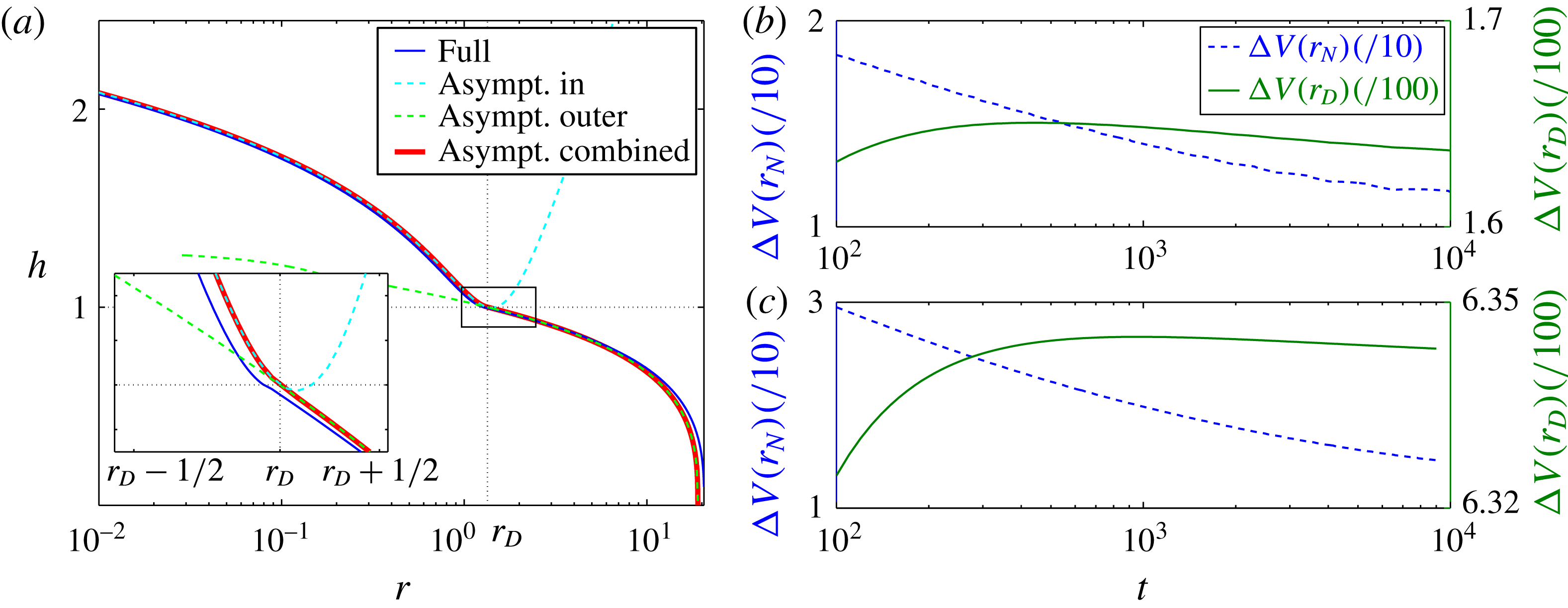
(a) Numerical solutions of the full equations for the thickness
 $h$
for
 ${\it\lambda}=0.1$
,
 $\mathscr{Q}=1$
at time
 $t=10^{3}$
(—— blue) and the corresponding asymptotic solutions for
 $r<r_{D}$
(– – – – cyan), and for
 $r>r_{D}$
(– – – – green). The solution that results from matching at
 $r_{D}$
is marked by (—— red). Insets zoom into the vicinity of the drainage front. (b,c) The evolution of the volume difference normalised by the total volume, between the numerical and asymptotic solutions of the percolating region
 $r\leqslant r_{D}$
(—— olivegreen) and of the whole current
 $r\leqslant r_{N}$
(– – – – blue), for
 $\mathscr{Q}=1$
(b) and
 $\mathscr{Q}=10$
(c).

In the limit
 ${\it\lambda}\ll 1$
we obtain closed-form solutions by matching (2.17b
) with the approximation (2.23),
 $$\begin{eqnarray}\displaystyle 1=-2(2\mathscr{Q}-r_{D}^{2})\ln \sqrt{\frac{r_{D}^{2}}{{\it\zeta}_{N}^{2}(2{\rm\pi}\mathscr{Q}-{\rm\pi}r_{D}^{2})^{3/4}t}}, & & \displaystyle\end{eqnarray}$$
implying that
 $r_{D}\rightarrow \sqrt{2\mathscr{Q}}$
for
 $t\gg 1$
, which is consistent with the steady-state solution with
 $\mathscr{Q}_{D}=0$
(2.17b
). When
 $r_{D}\ll \sqrt{2\mathscr{Q}}$
we predict that
 $r_{D}\approx {\it\zeta}_{N}(2{\rm\pi}\mathscr{Q})^{3/8}t^{1/2}e^{-1/4\mathscr{Q}}$
, which is consistent with the early-time behaviour (2.15a
) up to a constant factor. Another analytical form with higher accuracy can be obtained using the approximation (2.21)
 $$\begin{eqnarray}\displaystyle 1={\it\zeta}_{N}^{2/3}(2{\rm\pi}\mathscr{Q}-{\rm\pi}r_{D}^{2})^{1/4}{\it\psi}\left(\sqrt{\frac{r_{D}^{2}}{{\it\zeta}_{N}^{2}(2{\rm\pi}\mathscr{Q}-{\rm\pi}r_{D}^{2})^{3/4}t}}\right), & & \displaystyle\end{eqnarray}$$
which is also consistent with
 $r_{D}\rightarrow \sqrt{2\mathscr{Q}}$
for
 $t\gg 1$
(figure 3
a). This late-time asymptotic solution predicts the early-time behaviour of the two fronts to high accuracy, and it also predicts quite accurately the early-time evolution of
 $\mathscr{Q}_{D}$
in limit
 $\mathscr{Q}\ll 1$
.
For general
 ${\it\lambda}$
the asymptotic closed-form relation (2.17b
) is no longer valid. In this case, we obtain an asymptotic relation for the inner part by solving the system (2.16) for a specified range of
 $\mathscr{Q}_{D}$
and a given
 ${\it\lambda}$
, which leads to a numerical mapping between
 $r_{D}$
and
 $\mathscr{Q}_{D}$
that generalizes (2.17b
) for any
 ${\it\lambda}$
. Matching this asymptotic prediction for the inner region with that of the outer region provides a better agreement with the full numerical solution for small but finite
 ${\it\lambda}$
(figures 2
b, 3, black dash line), and shows very good agreement with the early and late-time evolution of the full numerical solution for larger values of
 ${\it\lambda}$
(figure 4). It should be noted that as the flux to the exterior current
 $\mathscr{Q}_{D}$
reaches it’s asymptotic form, there is an additional time needed for the fluid front
 $r_{N}$
to attain the corresponding position. This results in the excellent agreement by
 $t=10^{4}$
in figures 3(b) and 4(c), and the much slower approach to the asymptotic solution for
 $r_{N}$
in figures 2(b) and 4(a).
Together with the corresponding solution for
 $\mathscr{Q}_{D}(t)$
and
 $r_{D}$
, we determine the thickness
 $h$
and the front
 $r_{N}$
following the similarity solution for a gravity current on impermeable surface, which results in the quasi-self-similar solution
 $$\begin{eqnarray}\displaystyle & \displaystyle h(z,t)={\it\zeta}_{N}^{2/3}[2{\rm\pi}\mathscr{Q}_{D}(t)]^{1/4}{\it\psi}(z), & \displaystyle\end{eqnarray}$$
 $$\begin{eqnarray}\displaystyle & \displaystyle r_{N}={\it\zeta}_{N}[2{\rm\pi}\mathscr{Q}_{D}(t)]^{3/8}t^{1/2}, & \displaystyle\end{eqnarray}$$
 $\mathscr{Q}_{D}$
that is absent in the classical solution for a gravity current on impermeable substrate. Overall, we find that the asymptotic predictions of
 $r_{N},r_{D},\mathscr{Q}_{D}$
and
 $h$
are in good agreement with the full numerical solution (figures 2–4 and 6). We estimate the convergence to the asymptotic solution by computing the evolution of the normalised volume difference of the numeric and asymptotic solutions
 $$\begin{eqnarray}\displaystyle {\rm\Delta}V(r_{i})=\frac{\displaystyle \int _{0}^{r_{i}(t)}r|h(t)_{numeric}-h(t)_{asymptotic}|\,\text{d}r}{\displaystyle \int _{0}^{r_{i}(t)}rh(t)_{numeric}\,\text{d}r}, & & \displaystyle\end{eqnarray}$$
where
 $r_{i}=r_{D}$
or
 $r_{N}$
(figure 6
b,c). This indicates that by
 $t=10^{4}$
the convergence of the interior current (
 $r\leqslant r_{D}$
) can be 10 times better than that of the exterior current, which again demonstrates the time needed for the exterior flow to adjust to changes that occur near the draining front.
3 Experimental validation
To test the theoretical results we have conducted a series of laboratory experiments in which a viscous fluid was injected onto a thin, perforated metal plate. The resultant viscous gravity currents propagated along, and drained through, the thin porous plate allowing direct comparison with our theoretical model. The viscous fluid used was Lyle’s golden syrup mixed with water to modify the viscosity and with titanium dioxide (
 $0.2$
% in weight) to make the fluid optically opaque for imaging. Perforated sheets of steel were used as the porous substrate, with a thickness of
 $b=0.75~\text{mm}$
and pore diameter
 $d_{p}=1$
or 2 mm. To fully characterize the system we first conducted a suite of drainage experiments, described in § 3.1, in which we measured the effective permeability of the porous plate. This enables us to make quantitative predictions of the propagation and drainage from viscous gravity currents in § 3.2. Experiments took no more than a few minutes each and there were no significant heat sources near the apparatus. Therefore, within an experiment we assume that temperature variations were negligible and that quantities such as viscosity and surface tension were uniform and remained constant.
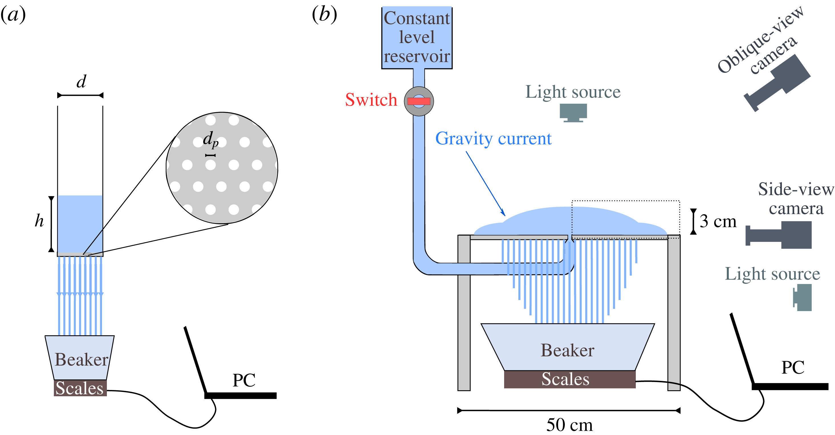
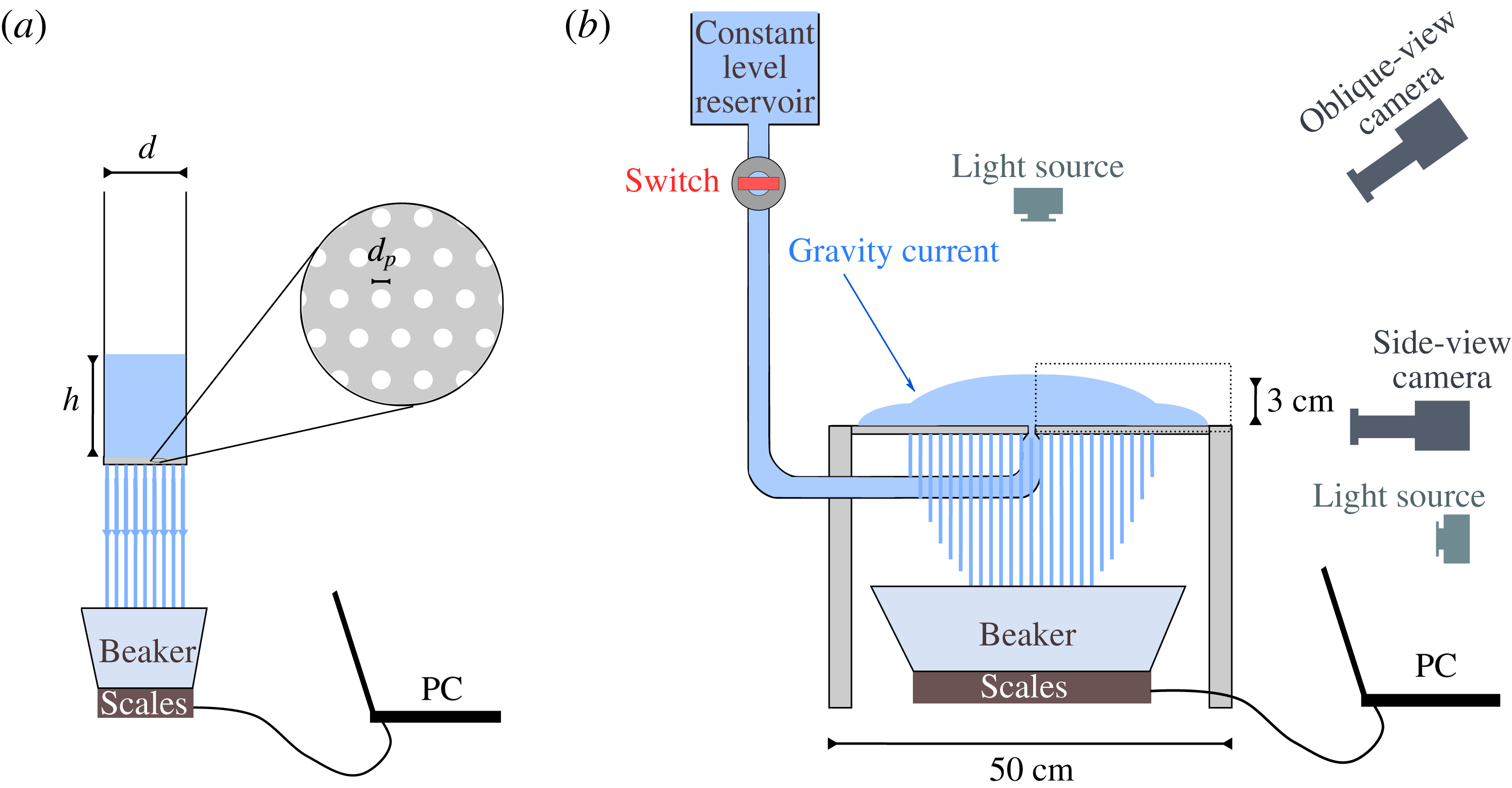
Diagrams of the experimental apparatus. (a) Apparatus to measure the permeability of the substrate is composed of a cylindrical tube of diameter
 $d$
with an open end at the top and a bottom end made of a steel mesh of thickness
 $b$
and holes of diameter
 $d_{p}$
. Viscous fluid that was contained in the cylinder drained across the mesh into a beaker whose mass was monitored. (b) In an apparatus for a gravity current over a porous substrate the same fluid is discharged at constant flux over an identical mesh. The evolution of the current was imaged from oblique and side views via synchronized cameras, and the drainage flux was monitored throughout the experiment. To acquire a side view of the drainage pattern, an additional light source was required. A zoom into the cross-section of the gravity current inside the dotted rectangular is schematically shown in figure 1.
3.1 Measuring the permeability of the substrate
The permeability of a porous plate templated by a regular lattice of cylindrical holes should, in principle, be amenable to robust theoretical estimates. However, since the mesh is thin compared with the pore diameter, any putative Poiseuille flow through the pores may not be fully developed and the detachment or dripping of fluid from the base may similarly affect the flux. Hence, an empirical characterization of the permeability is required.
The experimental apparatus consisted of a cylindrical tank of diameter
 $d=9.3$
cm that had an open end at the top and a bottom end that was covered with a disk of the perforated sheet of thickness
 $b$
(figure 7
a). We mounted the cylinder vertically and filled it with the viscous fluid to height
 $h_{0}>h_{D}$
, while its bottom end was covered with a removable seal. At
 $t=0$
we removed the seal abruptly, allowing the fluid to drain through the mesh into a beaker placed on the scales that monitored its weight
 $m$
. The instantaneous mass of the fluid in the cylinder is therefore
 $M(t)=M_{0}-m(t)$
, where
 $M_{0}={\rm\pi}d^{2}{\it\rho}h_{0}/4$
is the initial mass, so that the evolution of the height in the cylinder is
 $h(t)=h_{0}(1-m(t)/M_{0})$
by mass conservation. By the time the fluid level reached the bottom of the cylinder, a thin film remained attached to the walls of the cylinder with mass initially equal to approximately 15 % of
 $M_{0}$
. We accounted for that loss by using
 $\overline{M_{0}}\equiv m(t_{final})$
instead of
 $M_{0}$
in the computation of the evolution of the hydrostatic head that drives the flow,
 $$\begin{eqnarray}\displaystyle h(t)=h_{0}\left(1-\frac{m(t)}{\overline{M_{0}}}\right). & & \displaystyle\end{eqnarray}$$
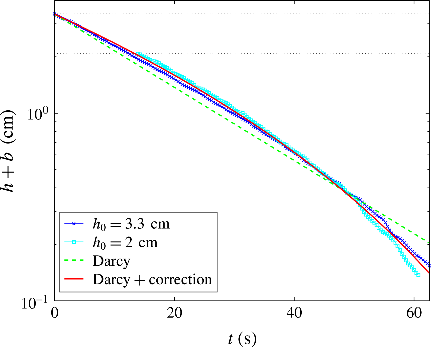
The experimental measurements, plotted as
 $h(t)$
in figure 8 imply a nearly exponential behaviour. The evolution of the height of the fluid column in the cylinder can be predicted using conservation of mass,
 $$\begin{eqnarray}\displaystyle \frac{\partial h}{\partial t}=-v_{p}=-{\it\phi}\frac{kg}{b{\it\nu}}(h+b), & & \displaystyle\end{eqnarray}$$
which has an exponential solution
 $$\begin{eqnarray}\displaystyle h(t)=(h_{0}+b)e^{-{\it\tau}t}-b, & & \displaystyle\end{eqnarray}$$
where
 ${\it\tau}={\it\phi}kg/b{\it\nu}$
is the characteristic drainage time. Using a viscometer we found the kinematic viscosity to be
 ${\it\nu}=31.66\pm 0.06~\text{cm}^{2}~\text{s}^{-1}$
. We then obtained the effective permeability
 ${\it\phi}k$
by computing a regression to the experimental data (figure 8), which resulted in an expected difference from the simple Darcy drainage model. The pore Reynolds number in this case is estimated as
 $$\begin{eqnarray}\displaystyle Re=\frac{vd_{p}}{{\it\nu}}\simeq 10^{-3}, & & \displaystyle\end{eqnarray}$$
where we take
 $v=0.2~\text{cm}~\text{s}^{-1}$
and
 $d_{p}=0.1~\text{cm}$
, implying that the flow should be well within Darcy’s regime. The discrepancy from Darcy’s law is therefore introduced through additional, weaker processes beside percolation. A potential cause is the interaction of the viscous fluid that emerges out of the base of the substrate with an air interface that is present under the substrate. Owing to strong capillary interactions along that interface the detachment of fluid from the substrate becomes complex, involving drops and jets in a spatio-temporally varying pattern, which appears to be stochastic (Pirat et al.
Reference Pirat, Mathis, Maïssa and Gil2004).
Evaluation of the permeability
 $k$
from one-dimensional percolation experiments using the apparatus shown in figure 7(a). Experiments were initiated with heads
 $h_{0}=3.3$
, 2 cm (
 $\times$
and ▫, respectively). Uncertainties of the thickness measurements are of the order of
 $10^{-2}~\text{cm}$
. Regression is computed initially using Darcy’s law (– – – –), and then using an effective percolation law (3.5), which is Darcy to leading order (——).

Given that the leakage follows Darcy’s law to leading order, we account for the complex drainage pattern by specifying an effective percolation law of the form
 $$\begin{eqnarray}\displaystyle \overline{v_{p}}\equiv -{\it\tau}(h+b)^{1-n}, & & \displaystyle\end{eqnarray}$$
where the parameter
 $n$
, to be found by regression, is expected to be smaller than 1 since the percolation is expected to follow Darcy flow to leading order. The solution to (3.2) with the effective percolation (3.5) is
 $$\begin{eqnarray}\displaystyle h=[n(h_{0}+b)-n{\it\tau}t]^{1/n}-b, & & \displaystyle\end{eqnarray}$$
and regression to the experimental data with
 $n$
as an additional free parameter results in
 ${\it\phi}k\approx 10^{-4}\pm 5\times 10^{-7}\times \text{cm}^{2}$
and
 $n\approx 0.26\pm 0.014$
(uncertainties represent the 95 % confidence interval), which is consistent with our expectation of
 $n<1$
(see figure 8). The percolation law may therefore be approximated as
 $$\begin{eqnarray}\displaystyle \overline{v_{p}}=-{\it\tau}(h+b)[1-n\log (h+b)]+O(n^{2}), & & \displaystyle\end{eqnarray}$$
which reflects a Darcy behaviour to leading order and a correction proportional to
 $n$
that is likely introduced by the complex leakage pattern at the bottom of the porous plate. The first-order correction to the percolation law is included in the full numerical simulation that predicts the experiments performed in the following section.
3.2 Gravity current experiments
We conducted a suite of experiments of viscous gravity currents propagating over a thin porous mesh, the results of which are summarized in table 1. The experimental apparatus consisted of a fluid reservoir, which provided a constant hydraulic head and hence constant flow rate, and a horizontal, perforated sheet of steel
 $(50\times 50~\text{cm}^{2})$
, identical to the one used in § 3.1, on which the injected fluid could propagate (figure 7
b). Experiments were initiated by turning a valve on, which discharged fluid from the reservoir through a circular nozzle 15 mm in diameter and located in the centre and at the same level of the perforated sheet. The relatively small thickness of the perforated sheet that we used
 $(b=0.75~\text{mm})$
compared with its length (500 mm across), resulted in some deformation of the substrate due to the weight applied by the propagating current. Deformation of the substrate often lead to local variations in the thickness of the current, and hence to variations in the local leakage flux through the porous plate, both of which resulted in some currents propagating in a non-axisymmetric mode (see figure 13 for example). To keep the thin perforated sheet flat, we suspended the thin substrate from below and above at several locations with fishing line. This provided a support to the substrate, in addition to the support at the centre of the sheet by the nozzle and along its rim by a transparent frame.
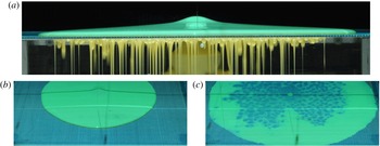
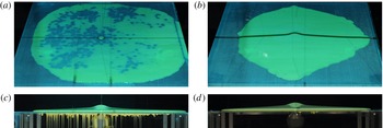
Snapshots from experiment A (table 1) of a viscous gravity current over a porous substrate with finite entry pressure. (a) Side view of the current showing the surface current and the draining fluid underneath the substrate and the gap between the positions of the drainage and the fluid fronts. (b) An oblique view of the surface current at the time corresponding to that of the image in (a). (c) An oblique view of the substrate at the end of the experiment (
 $Q=0$
), showing the inner region where drainage was active and the outer ring of fluid that has not broken through the critical entry pressure.

With this experimental arrangement, the viscous fluid propagated axisymmetrically over the perforated sheet, and leaked through the sheet, where the capillary entry pressure was exceeded. The drained fluid was collected in a beaker whose weight was continuously monitored. The evolution of the current was imaged by a side view camera that was aligned with the plane of the substrate so that it captured both the surface current and the draining fluid (see figure 9 a). Another camera took images from an oblique angle above the substrate (figure 9 b,c). Both cameras operated at a rate of 2 frames per second and were triggered simultaneously.
In preliminary experiments, we tested two types of perforated sheets having pore diameters
 $d_{p}=1$
and 2 mm. This property appeared to have a large effect on the entry pressure (2.6) and on the percolation through the substrate (3.4). In experiments using the larger pore-diameter sheet, we could not access conditions in which there was a measurable difference between the drainage and the fluid fronts, suggesting a small or negligible capillary entry pressure. In contrast, using the smaller pore-diameter sheet leakage had hardly initiated by the time the fluid front had reached the edge of the apparatus, suggesting that the capillary entry pressure was too large for leakage to occur. Therefore, in order to observe and measure the intermediate regime, in which
 $0<r_{D}<r_{N}$
, we used the sheet with the smaller pore diameter and partially prewet it with a small volume of water (smaller than the total pore volume) which was sprayed uniformly on the substrate before the initiation of an experiment. We emphasise that the surface tension coefficient of the fluid used for partial prewetting is smaller by 10 % with respect to the current fluid. We found that the partial prewetting of the porous sheet had the effect of producing an intermediate critical depth.
Parameters of the gravity current experiments.

We performed several experiments as shown in table 1. For each experiment we obtained a series of side-view snapshots (e.g. figure 9
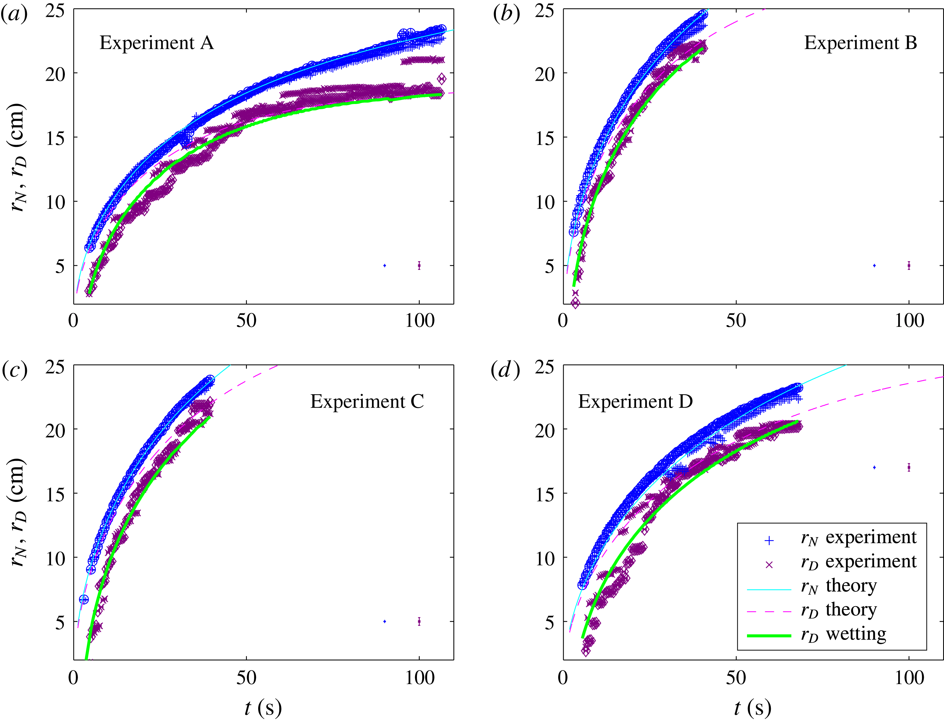
a), from which we measured the evolution of the drainage and of the fluid fronts (figure 10). The side-view images (see supplementary movie 1 available at http://dx.doi.org/10.1017/jfm.2016.412) reveal a complex leakage pattern through the substrate, showing drops and jets that alter spatio-temporally throughout the experiment. The oblique-view camera (see also supplementary movie 2) was used to confirm the axisymmetry of the flow throughout the experiment (e.g. figure 9
b), but it also revealed other aspects of the complex leakage pattern (figure 9
c), which we discuss in the next section. The measurement error of
 $r_{N}$
, defined as half the width of the region over which the fluid colour transits to the background colour, is approximately 1 mm. Measurement error of
 $r_{D}$
, defined as half the width of a fluid jet or drop, is approximately 3 mm. The temporal uncertainty of each measurement, estimated as half the interval between two successive images, is approximately 0.25 s.
In most of the experiments the current could not evolve to the late-time phase in which the drainage front reached a steady position since the extent of
 $r_{D}$
was comparable to the size of the apparatus. However, in experiment A (figure 10
a) we were able to measure a significant deceleration of the drainage front, which indicates an approach to a steady position. These experiments also indicated that the early-time evolution of the fluid front followed the expected
 $t^{1/2}$
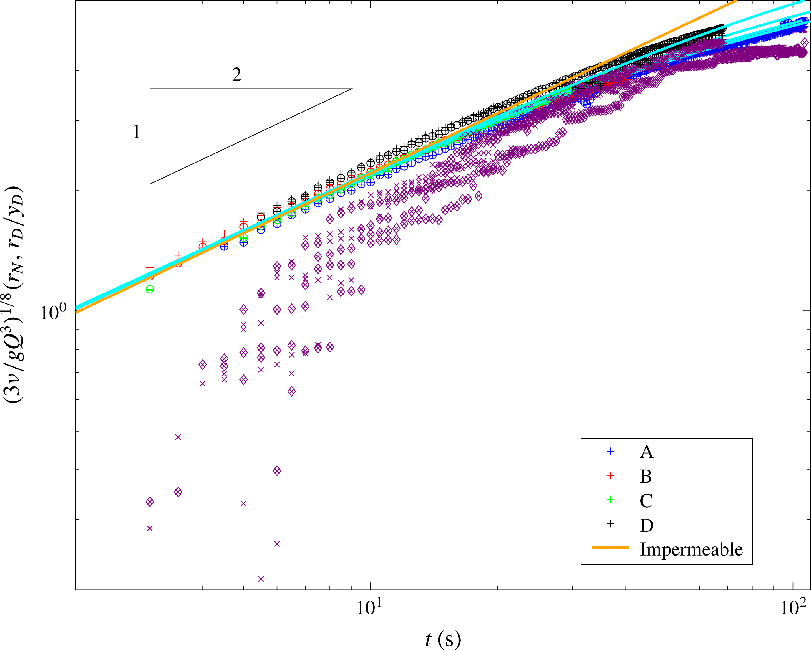
power law, while the detailed dynamics of fluid invasion into the pores and detachment of drips from the underside of the porous plate (neither of which we attempt to capture in the simple theory) resulted in a drainage front which did not exhibit power-law behaviour (figure 11). More precisely, the drainage front seemed to lag behind the theoretical value at early time, despite having a larger acceleration.
Experimental measurements and theoretical predictions of
 $r_{N}$
(○,
 $+$
) and
 $r_{D}$
(♢,
 $\times$
) for gravity currents with parameters given in table 1, where the two symbols denote the left and the right fronts (see figure 9
a) respectively. Error bars for
 $r_{N}$
and
 $r_{D}$
are shown on the bottom right corner in corresponding colour. The theoretical predictions are marked with —— (cyan) and – – – – (magenta) for the fluid and drainage fronts. A correction to the early-time evolution of the drainage owing to finite-time wetting of the substrate is marked with —— (green).

To quantitatively compare the experimental results with the theoretical predictions, we computed the numerical solution for the dimensionless parameter
 $\mathscr{Q}$
and
 ${\it\lambda}$
specified in table 1, accounting for the non-Darcy correction to the percolation law (3.7). Estimating the dimensionless quantities requires determination of the value of the critical entry thickness
 $h_{D}$
, and particularly the quantity
 $4{\it\gamma}\cos {\it\theta}$
in (2.6). Since the fluid is over 99 % Lyle’s golden syrup, the surface tension coefficient is approximately
 ${\it\gamma}\approx 80~\text{dyn}~\text{cm}^{-1}$
(Llewellin, Mader & Wilson Reference Llewellin, Mader and Wilson2002), which is similar to the surface tension coefficient of water
 $(72~\text{dyn}~\text{cm}^{-1})$
. We therefore make the assumption that the contact angle of golden syrup on steel is similar to that of water on steel. The latter can vary significantly depending on the substrate surface energy and texture (e.g.
 $55{-}97^{\circ }$
(Boulange-Petermann, Gabet & Baroux Reference Boulange-Petermann, Gabet and Baroux2006); conversion from advancing and receding to Young contact angles following Tadmor (Reference Tadmor2004)), implying that
 $h_{D}$
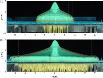
may be in the range of 1–13 mm, which is consistent with our observation (see for example, figure 12
b). Within that range we use the contact angle as a tuning parameter to fit the theoretical predictions.
Measurements of the fronts
 $r_{N}$
(
 $+,\circ$
, blue, red, green and black) and
 $r_{D}$
(♢,
 $\times$
), where the two symbols denote the left and the right fronts, of gravity currents with parameters given in table 1, normalized with respect to the early time solutions (2.14b
) and (2.15a
) respectively. The solution for a constant-flux gravity current on an impermeable surface (—— orange) is shown for reference, and the theoretical predictions for the fluid front
 $r_{N}$
are shown (—— cyan).

The source flux
 $Q$
was measured by two methods. The first was based on measuring the drained mass of fluid, in a manner similar to the method described in § 3.1. However, this measures
 $Q-Q_{D}$
and in most experiments the drainage front did not reach its asymptotic value
 $r_{D}(t\rightarrow \infty )$
and therefore a credible measurement of
 $Q$
could not be achieved with this method. A method that produced a more reliable measurement was based on the known solution for a gravity current on impermeable substrate (Huppert Reference Huppert1982). Specifically, as long as the flux through the substrate is small compared with
 $Q$
, which is the case in early time, the fluid front should follow to leading order the early-time solution (2.14b
), which in dimensional form is
 $$\begin{eqnarray}\displaystyle r_{N}={\it\xi}_{N}\left(\frac{gQ^{3}}{3{\it\nu}}\right)^{1/8}t^{1/2}. & & \displaystyle\end{eqnarray}$$
Scaling
 $r_{N}$
by the coefficient of the right-hand side of (3.8), should therefore result in the collapse of the measurements of all the experiments to a single curve
 ${\it\xi}_{N}t^{1/2}$
. Using the quantities we measured (table 1) we find that indeed measurements of
 $r_{N}$
of all the experiments scale at
 $t^{1/2}$
during the early-time evolution and that by fitting
 $Q$
they collapse to the same curve (figure 11). This early-time collapse therefore supports our analysis that leakage is initially a secondary effect, and provides a robust estimate of the input flux which can be subsequently used to test our model predictions against the experimental data in the region where leakage plays a leading-order role. The fitted values for
 $Q$
differ from the measurements of the flux via the drained-fluid method by 9 % in the case of experiment A, in which the drainage front decelerated substantially compared with the other experiments. In contrast, the drainage front in the other experiments was far from its steady-state limit and so the difference in the measurement of
 $Q$
between the two methods was larger (28 % for experiments B and D and 40 % for experiment C).
Obtaining the flux for each experiment using (3.8), we then use the critical capillary entry pressure to fit both the drainage and the current fronts along the entire temporal interval. The results of the comparison show good agreement between theory and measurements for the fluid front and for the late-time evolution of the drainage front (figure 10). A corresponding comparison of the current thickness also demonstrates consistency between the theory and the experiments (figure 12).
Snapshots from side view from experiment A (table 1) at
 $t=10~\text{s}$
(a) and at
 $t=100~\text{s}$
(b). The theoretical prediction of
 $h$
is shown (——) and the corresponding predictions of the drainage fronts are shown in – – – – (red) for the wetting-excluded theory and in – – – – (green) for the delayed-wetting correction. The position
 $z=0$
is the top surface of the substrate at the centre (– – – – yellow).

As indicated earlier, a discrepancy exists between the theory and the measured evolution of the drainage front
 $r_{D}$
at early times. The difference between the predicted and measured values is larger than the error in the measured position (figure 10), which implies that additional physical processes need to be accounted for in the initial drainage. Before an experiment initiates, the pores of the substrate contain air. Once the critical depth is reached and leakage initiates, the fluid wets the pores of thickness
 $b$
, and pushes the air away. After that wetting phase, when the pores are saturated with the viscous fluid, the percolation is governed by the effective Darcy’s law (3.7). The simplified theory in § 2.1 accounts for the percolation of a saturated porous substrate but does not include a description of this initial wetting process. We therefore include a delay term in the propagation of the drainage front in the original, wetting-excluded theory, accounting for fluid filling the pore space. We assume that the delay term is proportional to the velocity of the drainage front and has a characteristic time scale denoted by
 $\mathscr{T}$
. Specifically, the difference between the predicted and measured positions of the drainage front is
 $$\begin{eqnarray}\displaystyle r_{D}^{predicted}-r_{D}^{measured}={\dot{r}}_{D}\mathscr{T}. & & \displaystyle\end{eqnarray}$$
Fitting (3.9) to the experimental measurements of the drainage front with
 $\mathscr{T}$
as a free parameter results in a much better agreement with the experiments (figure 10), where the characteristic delay time is
 $\mathscr{T}=4.85\pm 0.97~\text{s}$
(table 1). This time interval is comparable to the percolation time scale
 $b{\it\nu}/{\it\phi}kg\approx 20~\text{s}$
.
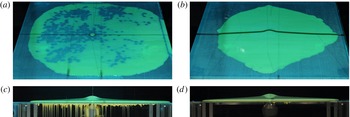
Snapshots from several experiments that we did not include in the analysis. In these experiments drainage was either non-uniform or did not initiate, possibly because the porous substrate was not sufficiently levelled or because the entry pressure was too high. (a) Snapshot after the termination of an experiment in which percolation did not initiate on the right half. (b) Strongly non-axisymmetric surface front, (c) Side view of the experiment in (a) at an earlier time, showing weaker drainage on the right side. (d) Side view of an experiment where percolation did not initiate throughout the flow.
4 Discussion
The theoretical, numerical and experimental investigation of the previous sections have demonstrated that finite capillary entry pressure can have a leading-order effect on the drainage of viscous fluids into porous substrates. Previous studies, in which there was no capillary entry pressure, have shown that a finite extent is reached for either two-dimensional or axisymmetric spreading (e.g. Pritchard et al. Reference Pritchard, Woods and Hogg2001; Spannuth et al. Reference Spannuth, Neufeld, Wettlaufer and Worster2009). This steady state is reached when the input flux is balanced by the leakage flux, and is characterized by having a zero fluid depth at the drainage front of the current. In stark contrast, for the currents considered here, the finite capillary entry pressure imposes a finite current depth at the edge of the drainage region. As a consequence, there is always a residual flux of fluid beyond the region of leakage, and hence a viscous current propagating into the far field. The implication being that, despite a leading order balance between the input flux and leakage, fluid continues to propagate far from the injection point.
Evaluation of the experiments in § 3.2 using the viscous theory presented in § 2 demonstrates the influence of the capillary entry pressure in restricting leakage to a finite region beyond which an undraining current continues to propagate. However, this evaluation requires a validation that the underlying assumptions of the theory are satisfied during the experiment. Particularly,
 $Re\ll 1$
has to be satisfied throughout the flow. We evaluate
 $Re$
at the nozzle, assuming that it represents an upper limit to
 $Re$
throughout the flow. The nozzle has a cone shape that fits the feeding pipe of radius
 $\bar{R}$
at one edge, and has a narrower edge of radius
 $R$
, from which the fluid is discharged at velocity
 $U$
onto the perforated sheet. The flux
 $Q$
from the feeding pipe and into the nozzle can be estimated via Poiseuille’s law
 $Q={\rm\pi}\bar{R}^{4}{\rm\Delta}p/8{\it\nu}{\it\rho}L$
, where
 $L$
is the length of the feeding pipe,
 ${\rm\Delta}p={\it\rho}g\bar{b}$
is the pressure drop and
 $\bar{b}$
is the head. Conservation of mass implies that
 $U=Q/{\rm\pi}R^{2}$
, therefore
 $Re$
at the nozzle outlet is
 $$\begin{eqnarray}\displaystyle Re=\frac{UR}{{\it\nu}}=\frac{g\bar{b}\bar{R}^{4}}{8L{\it\nu}^{2}R}. & & \displaystyle\end{eqnarray}$$
Using
 $\bar{b}=22~\text{cm}$
,
 $\bar{R}=1.27~\text{cm}$
,
 $R=0.75~\text{cm}$
,
 $L=120~\text{cm}$
, and
 ${\it\nu}=20~\text{cm}^{2}~\text{s}^{-1}$
the lowest kinematic viscosity, we find that
 $Re\approx 0.2$
. Moreover, a valve that was positioned between the head and the feeding pipe was only partially open, so the flux in our experiments was lower than the maximum that the system could provide. Therefore the actual upper limit on
 $Re$
was even lower than that estimated above, which confirms that our experiments were well within a viscous-dominated regime.
A major component of the discrepancy between our theory and experiments is the initial flow through the porous substrate. The finite thickness of the substrate resulted in additional capillary interactions between the viscous fluid and the underlying layer of air. This led to an apparent stochastic pattern of leakage, involving complex interactions of drops and jets that vary spatio-temporally along the bottom side of the metallic mesh. A reflection of that complex leakage is also seen in the oblique angle images that were taken after the termination of experiments, which revealed a non-axisymmetric drainage front and a leakage region composed of a distributed spot pattern (figure 9
c). These spots, having a typical diameter of
 ${\sim}10$
pore diameters, were regions where fluid was either completely drained or was suspended on the substrate in a very thin and transparent layer of fluid. This pattern of leakage may contribute to the non-Darcy percolation that we measured, and although it seem to introduce a relatively small correction to Darcy’s law, such interactions may become important in other set-ups (Pirat et al.
Reference Pirat, Mathis, Maïssa and Gil2004).
Additional discrepancy in the early time evolution of the drainage front was attributed to the finite wetting time of the partially prewetted pores. This resulted in a time delay, which implied a significant correction to the prediction of the drainage front position. However, we expect this delay to be less important to the propagation of the fluid front because the delay is mostly significant in early time, in which most of the fluid flux contributes to the surface current. We note that the solubility of syrup and water could modify the viscosity of the draining fluid and impact the flow time scales. This may be a source of discrepancy if the solubility time scale, which is difficult to quantitatively constrain, is short compared with the time scale of wetting of the partially water-prewetted pores by the syrup that is approximately given by the delay time scale
 $\mathscr{T}\approx 5~\text{s}$
. We should also emphasize that the wetting-induced delay was not an issue in the measurement of permeability (§ 3.1) because in that case the substrate pores became saturated by the time the experiment was initiated. Future studies should account for the wetting phase in more detail, taking into account the spreading of the fluid in the cylindrical pores (e.g. Davis & Hocking Reference Davis and Hocking2000).
5 Conclusions
The propagation of a viscous gravity current over a porous substrate with finite entry pressure results in two distinguished flow regimes; an inner domain in which drainage through the substrate is active and an outer domain in which there is no drainage. Consequently, the flow involved two time-dependent fronts, one at the interface between the two regions and another at the nose of the current. An asymptotic analysis near the drainage front turns out to be powerful in predicting the evolution of the entire current at early, intermediate and late times. Specifically, we find that the draining portion of the current approaches a steady-state solution logarithmically in time, which can be approximated quite accurately by solving a steady-state boundary value problem. In addition, the non-draining part has a quasi-self-similar solution, which has an identical structure to the self-similar solution of gravity current on impermeable surface (Huppert Reference Huppert1982), but with a time-dependent input flux. This implies that in the flow we consider, the front of the surface flow would, in principle, never stop. The experiments revealed additional physical processes that may be important in a number of practical applications, including stochastic leakage pattern at the exit of the porous substrate and a significant leakage delay despite the relatively thin substrate that was used. Accounting for these processes we find that our theory is consistent with the experimental measurements.
The main result of this work is that when capillary forces inhibit fluid invasion into a porous substrate, fluid may propagate indefinitely even when the leakage flux and input flux balance to leading order. This result has implications for the region over which a spill may accumulate in industrial settings, and the distance over which environmental or geophysical flows may propagate.
Acknowledgements
We thank M. Hallworth, C. Hitch and D. Page-Croft for assisting with technical aspects of the experiment; Y. Ashkenazi for computational resources on Tsia; discussions with H. Huppert, J. Lister, S. S. Pegler, L. Prigozhin, I. Rubenstein, M. G. Worster, B. Zaltzman. R.S. thanks SIDEER and BIDR in Ben-Gurion University, Israel, for financial support, and to DAMTP, University of Cambridge, UK, where some of this research took place. J.A.N. acknowledges support from a Royal Society University Research Fellowship.
Supplementary movies
Supplementary movies are available at http://dx.doi.org/10.1017/jfm.2016.412.
Appendix A. The numerical solver
Solving equations (2.10) on a single domain
 $r\in [0,r_{N}]$
is computationally expensive if we wish to investigate the long-time asymptotic behaviour, as the moving front requires a growing number of nodes with time. Instead, we split the domain into two sub domains at the interface
 $r=r_{D}$
, map each of the subdomains into the interval
 $[0,1]$
, in which the free boundaries become stationary positions, and solve (2.10) in the two subdomains simultaneously. Applying the mapping
 $r\rightarrow r/r_{D}$
in the percolating (inner) region (
 $0\leqslant r\leqslant r_{D}(t)$
), and
 $r\rightarrow (r-r_{D})/(r_{N}-r_{D})$
in the impermeable (outer) region (
 $r_{D}(t)<r\leqslant r_{N}(t)$
) leads to a partial differential equation for the evolution of the free surface in both domains
 $$\begin{eqnarray}\displaystyle & & \displaystyle \frac{\partial h}{\partial t}-\frac{\partial h}{\partial r}\frac{r{\dot{A}}+{\dot{B}}}{r_{I}(1-C)}-\frac{1}{r_{I}^{2}[r(1-C)+C](1-C)^{2}}\frac{\partial }{\partial r}\nonumber\\ \displaystyle & & \displaystyle \quad \times \,\left[(r(1-C)+C)h^{3}\frac{\partial h}{\partial r}\right]=-P({\it\lambda}h+1),\end{eqnarray}$$
where
 $r\in [0,1]$
. For the permeable regime we set
 $$\begin{eqnarray}\displaystyle r_{I}=r_{D},\quad {\dot{A}}={\dot{r}}_{D},\quad {\dot{B}}=0,\quad C=0,\quad P=1, & & \displaystyle\end{eqnarray}$$
and for the impermeable regime we set
 $$\begin{eqnarray}\displaystyle r_{I}=r_{N},\quad {\dot{A}}={\dot{r}}_{N}-{\dot{r}}_{D},\quad {\dot{B}}={\dot{r}}_{D},\quad C=\frac{r_{D}}{r_{N}},\quad P=0. & & \displaystyle\end{eqnarray}$$
The mapping into two fixed intervals requires two evolution equations, one for each front. The outer front evolves kinematically,
 $$\begin{eqnarray}\displaystyle {\dot{r}}_{N}=\frac{q}{h}=-\frac{1}{3(r_{N}-r_{D})}\left.\frac{\partial h^{3}}{\partial r}\right|_{r=1}, & & \displaystyle\end{eqnarray}$$
in terms of the mapped coordinates, where the spatial derivative is evaluated using the two nearest nodes and the boundary condition
 $h(r_{N})=0$
, thus providing second-order accuracy. For the inner front we obtain an evolution equation by taking the time derivative of the boundary condition (2.10c
) and then substituting
 $\partial h/\partial t$
with equation (2.10a
) for the drainage-active region, which in terms of the non-mapped coordinates becomes
 $$\begin{eqnarray}\displaystyle {\dot{r}}_{D}=-\left.\frac{\displaystyle \frac{1}{r}\frac{\partial }{\partial r}\left(rh^{3}\frac{\partial h}{\partial r}\right)-\left({\it\lambda}h+1\right)}{\partial h/\partial r}\right|_{r_{D}}. & & \displaystyle\end{eqnarray}$$
Second-order accuracy of the finite-difference representation of (A 4b ) is achieved more easily in the non-mapped space than in the mapped space. In addition to the front evolution equations, two more boundary conditions are needed together with the four boundary conditions (2.10b )–(2.10e ), to ensure continuity of thickness and flux at the joint interface, namely
 $$\begin{eqnarray}\displaystyle \unicode[STIX]{x27E6}h\unicode[STIX]{x27E7}=\unicode[STIX]{x27E6}q\unicode[STIX]{x27E7}=0\quad \text{at }r=r_{D}. & & \displaystyle\end{eqnarray}$$
We solve the evolution equations for the fronts and for the thickness in both domains simultaneously, using finite-volume discretization on a uniform grid and an implicit Crank–Nicolson scheme together with a predictor–corrector iteration to evaluate the nonlinear terms, and with adjustable time stepping. This scheme provides a second-order accuracy in both time and space for the solution of
 $h$
and for the position of the two fronts. However, since
 $q\propto \partial h/\partial r$
the accuracy of solution for the flux is only first order. To compensate for the loss of accuracy we enhance the grid density.
We confirmed that the numerical solver is consistent with closed-form analytical solutions of several kinds: (i) propagation of a current on impermeable substrate (
 $P=0$
everywhere; Huppert Reference Huppert1982), (ii) propagation of a current on a fully prewetted substrate (
 $P=1$
everywhere; Spannuth et al.
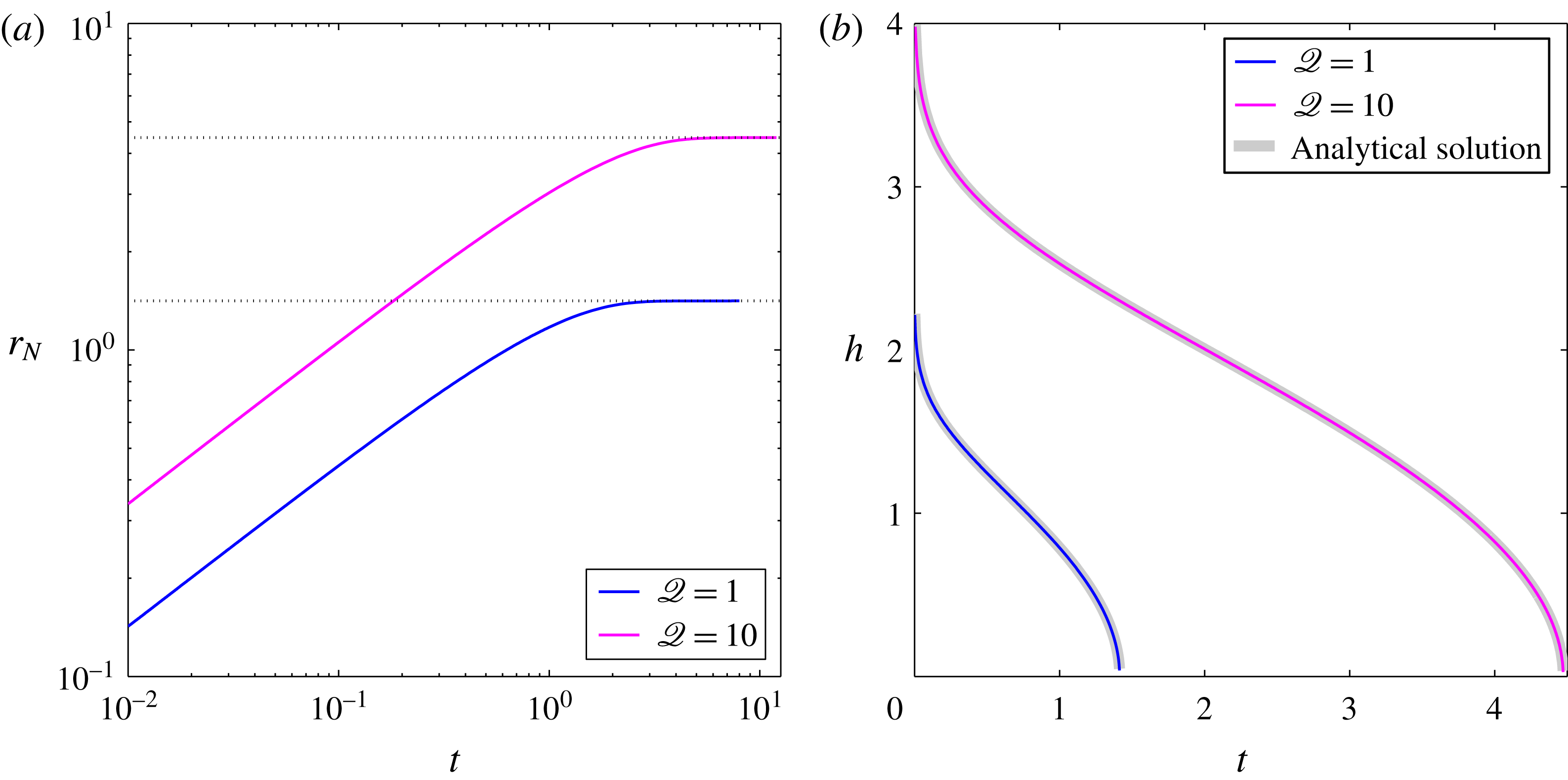
Reference Spannuth, Neufeld, Wettlaufer and Worster2009) as shown in figure 14 and (iii) the late-time asymptotic flow in the permeable region (figure 2
a).
Comparison of the numerical solutions of the full equations with the analytic solution for the fully prewetted substrate (Spannuth et al.
Reference Spannuth, Neufeld, Wettlaufer and Worster2009). To simulate that situation we set
 ${\it\lambda}=0$
,
 $\mathscr{Q}=1$
or 10 and
 $P=1$
, which prescribes the substrate to be permeable everywhere and sets the critical pressure to be zero. (a) The evolution of the fluid front
 $r_{N}$
reaches a steady value equal to
 $\sqrt{2\mathscr{Q}}$
(grid lines), as the theory predicts. (b) The numerical solution of the thickness (– – – – blue, – – – – magenta), compared with the analytical solution of Spannuth et al. (Reference Spannuth, Neufeld, Wettlaufer and Worster2009) (– – – – grey).