1. Introduction
Air pollution poses a major threat to human health and the environment worldwide. According to the recent reports on the state of global air (Health Effects Institute 2025, 2024), particulate pollution was responsible for an estimated 8.1 million deaths in 2021 and 7.9 million in 2023 globally. Particulate matter consists of tiny particles suspended in the air that can remain airborne for many hours to days, are easily inhaled, penetrate the lungs and have thus become a growing health concern (Anderson, Thundiyil & Stolbach Reference Anderson, Thundiyil and Stolbach2012; Lelieveld et al. Reference Lelieveld, Klingmüller, Pozzer, Pöschl, Fnais, Daiber and Münzel2019; World Health Organization 2021), particularly in densely populated urban areas. The movement of vehicles on the road generates both exhaust (e.g.
 ${\rm CO}_2,\;{\rm CO},\; {\rm SO}_{x},\; {\rm NO}_{x},\; {\rm VOCs},\; {\rm HCs}$
and
 $\rm PM$
(mostly soot)) and non-exhaust emissions and the latter is generated by the resuspension of particulates present on the road, like fine dust particles, brake wear and tyre wear (Piscitello et al. Reference Piscitello, Bianco, Casasso and Sethi2021). A recent study highlights the substantial role of vehicles in contributing to air pollution (Kumari, Jain & Elumalai Reference Kumari, Jain and Elumalai2021), emphasising the critical importance of studying pollutant dispersion in vehicle wakes. Vehicular movement causes the turbulent mixing of pollutants (could be active or passive) due to the wake produced, which increases pollutant levels in the environment. Recent research and pollution control policies have primarily focused on exhaust emissions, resulting in rigorous regulations and technological progress that have reduced the contribution of vehicular exhaust emissions (Nagpure et al. Reference Nagpure, Gurjar, Kumar and Kumar2016). However, the non-exhaust emissions are not regulated or controlled. Even with zero tailpipe emissions, traffic will continue to contribute to fine and ultrafine particulate pollutants through non-exhaust emissions. Despite this, the understanding of the pollutant dispersion behind a moving vehicle is limited, and this aspect requires attention.
To understand the pollutant dispersion behind moving vehicles, it is necessary to analyse the wake they generate. Identifying the dominant turbulent wake structures and the wake topology is essential for understanding the dispersion phenomenon. The turbulent flow structures behind the vehicle, the level of turbulence in the wake, the rear slant angle of the vehicle and the type of ground surface are the major factors influencing the dispersion characteristics of pollutants in the vehicle wake (Ahmed Reference Ahmed1981). Vehicle wakes are particularly challenging to study since these flows are highly separated, unsteady and turbulent (
 $\textit{Re}_L =U_o L/\nu \approx 10^5 {-} 10^6$
, where
 $U_o$
is typical vehicle velocity,
 $L$
is the length of the vehicle and
 $\nu$
is the kinematic viscosity of air). Therefore, it is challenging to understand the complex dynamics and the dispersion mechanisms that it causes. The wake of a moving vehicle on the road can be divided into two regions: a near wake (
 $x/H \leqslant 15$
) and a far wake (
 $x/H \geqslant 15$
), where
 $H$
represents the height of a typical vehicle and
 $x$
represents the distance downstream in the wake (Baker Reference Baker2001). The near wake consists of spanwise recirculation vortices inside a separation bubble and a pair of large-scale longitudinal trailing vortices that extend up to several vehicle heights (typically
 $\approx 10H$
), whereas the far wake is the region of decaying turbulence, which has no visible mean flow structure.
Schematic diagram of time-averaged three-dimensional flow structures in the wake of the Ahmed body. Figure redrawn from Ahmed, Ramm & Faltin (Reference Ahmed, Ramm and Faltin1984).

Simplified vehicle models are very useful for investigating the wake flow associated with more complex actual passenger vehicles. Since conducting experiments with a full-size vehicle with all their geometrical features is very difficult, among various simplified vehicle models (e.g. MIRA, Davis, Rover, Windsor, SAE, etc.), the ‘Ahmed body’ (Ahmed et al. Reference Ahmed, Ramm and Faltin1984) is one of the most widely studied reference vehicle models. It captures the essential flow features present in the wake of a typical passenger vehicle which are responsible for aerodynamic drag and pollutant dispersion. Ahmed et al. (Reference Ahmed, Ramm and Faltin1984) demonstrated the impact of the rear slant angle (
 $\phi$
) on flow topology and aerodynamic drag using force and pressure measurements (at
 $\textit{Re}_l= 42.9\times 10^6$
, the Ahmed body length (
 $l$
) based Reynolds number). They observed a significant drag peak at
 $\phi =30^\circ$
, which is termed the critical rear slant angle
 $(\phi _c)$
. The schematic of time-averaged flow features in the near wake for an Ahmed body with
 $\phi \leqslant 30^\circ$
is shown in figure 1. The schematic shows the recirculation region, which consists of two spanwise recirculation vortices (labelled as A and B in figure 1), a pair of longitudinal trailing vortices (referred to as C in figure 1) at the edges of the rear slant surface and a separation bubble located behind the rear vertical base (referred to as D in figure 1). The strength and the interactions of the spanwise vortices (A and B) are influenced by the rear slant angle (
 $\phi$
). Lienhart & Becker (Reference Lienhart and Becker2003) performed laser Doppler anemometry (LDA), hot-wire anemometry and smoke visualisation measurements in the Ahmed body near wake. The experimental results provided a detailed description of the wake flow structures and their evolution in the wake. Wang et al. (Reference Wang, Zhou, Pin and Chan2013) analysed the wake flow structures behind the Ahmed body (
 $\phi =25^\circ,\;35^\circ$
), fixed on a false floor (a raised floor in the wind tunnel) to avoid the interaction of the boundary layer formed on the wind tunnel ground with the flow underneath the Ahmed body. Particle image velocimetry (PIV) measurements were performed in three orthogonal planes at
 $\textit{Re}_h=U_{\infty }h/\nu =0.53\times 10^5$
(Ahmed body height
 $h$
based Reynolds number). The results highlighted the significant influence of vehicle ground clearance on the wake flow topology. Recently, Zhang, Zhou & To (Reference Zhang, Zhou and To2015) examined the unsteady flow structures in the Ahmed body wake in the high drag regime (
 $\phi =25^\circ$
). Extensive hot-wire and PIV measurements, along with flow visualisation, were conducted in a wind tunnel. A conceptual model was proposed for the wake flow structures. A conceptual model of wake flow structures (both steady and unsteady) behind the Ahmed body was proposed. Liu et al. (Reference Liu, Zhang, Zhang and Zhou2021) performed a similar investigation on the Ahmed body in low drag regime (
 $\phi =35^\circ$
) and presented a thorough picture of both steady and unsteady predominant coherent flow structures. Other studies investigating the wake topology of the Ahmed body are Tunay et al. (Reference Tunay, Sahin and Akilli2013, Reference Tunay, Sahin and Ozbolat2014), Venning et al. (Reference Venning, Lo Jacono, Burton, Thompson and Sheridan2015, Reference Venning, Lo Jacono, Burton, Thompson and Sheridan2017, Reference Venning, McQueen, Jacono, Burton, Thompson and Sheridan2022), Krajnović & Davidson (Reference Krajnović and Davidson2005), Sagharichi & Tachie (Reference Sagharichi and Tachie2025) and Moscato & Romano (Reference Moscato and Romano2025).
Although there has been extensive research focused on the flow topology and properties of the wake structure behind the Ahmed body, there are relatively few investigations into the dispersion in the vehicle wake, some of which are discussed below. Richards et al. (Reference Richards, Wright, Baker and Baxendale2002) studied the flow and dispersion in the near wake of a MIRA vehicle model. The flow structures in the near wake were measured using PIV and hot-wire anemometry, and the concentration of the tracer was measured using a flame ionisation detector. The experimental results show that tracer concentration is influenced by the velocity and turbulence fields in the vehicle wake. Gosse et al. (Reference Gosse, Paranthoën, Patte-Rouland and Gonzalez2006a
,
Reference Gosse, Patte-Rouland, Gonzalez and Paranthoënb
, Reference Gosse, Gonzalez and Paranthoen2011) conducted experimental investigations on passive scalar (heated air) dispersion in the near wake of the Ahmed body (
 $\phi$
=
 $5^\circ$
,
 $25^\circ$
and
 $40^\circ$
). Cold-wire thermometry measurements revealed that the rear slant angle significantly affects the scalar concentration distribution in the near wake. However, the scalar concentration measurements were conducted with a stationary ground configuration in the wind tunnel, and scalar dispersion was not quantified. Chan et al. (Reference Chan, Gosse, Zhou, Lee, Wang and Huang2008a
) studied pollutant dispersion in the wake of a vehicle model (different from the Ahmed body) placed on a false floor (or raised floor) to eliminate the influence of the stationary wind tunnel floor. They employed LDA to measure velocity fields and cold-wire thermometry to obtain tracer concentrations. The findings revealed that both the flow structures and pollutant dispersion in the near wake are strongly influenced by the rear slant angle and the exhaust jet conditions of the scalar. Rodriguez et al. (Reference Rodriguez, Murzyn, Mehel and Larrarte2020) investigated the dispersion of ultrafine particles (UFP) in the wake of an Ahmed body and highlighted that the size of the recirculation region plays an important role in influencing UFP dispersion in both the near- and far-wake regions. In a recent study, Mathur et al. (Reference Mathur, Cholemari, Veeravalli and Khare2024a
) conducted unsteady Reynolds-averaged Navier–Stokes (unsteady-RANS) simulations to investigate smoke particle dispersion in the wake of an Ahmed body with a rear slant angle of
 $\phi = 25^\circ$
, alongside wind tunnel experiments using smoke for dispersion pattern visualisation. The simulation results were compared with the experimental data for dispersion, showing that unsteady-RANS simulations captured the typical flow structures in the Ahmed body wake. However, while the vertical spread of the smoke was predicted reasonably well, the lateral dispersion was under-predicted. Mathur et al. (Reference Mathur, Cholemari and Veeravalli2024b
) investigated the particle dispersion in the turbulent wake of the Ahmed body with two rear slant angles (
 $\phi =25^\circ$
,
 $40^\circ$
). The scalar concentration fields were measured in the Ahmed body near wake (
 $x\leqslant 5H$
), with a fixed/stationary wind tunnel floor. The findings indicate that the concentration fields in the near wake are highly dependent on the rear slant angle (
 $\phi$
). The size of the recirculation region and the existence of trailing vortices in the near wake govern the dispersion of the scalar pollutants. Keita et al. (Reference Keita, Mehel, Fokoua, Murzyn, Taniere, Arcen and Diourte2023) performed unsteady-RANS simulations combined with Lagrangian particle tracking to study the dispersion of UFP in the wake of a square-back Ahmed body (
 $\phi = 0^\circ$
). Their results revealed a highly asymmetric concentration distribution in the near wake, primarily caused by the offset location of the exhaust pipe. Additionally, the peak particle concentration progressively decreased with increasing downstream distance from the vehicle model. Other studies related to pollutant dispersion in vehicle wakes can be found in Kanda et al. (Reference Kanda, Uehara, Yamao, Yoshikawa and Morikawa2006), Chan et al. (Reference Chan, Luo, Cheung and Chan2008b
), Dong & Chan (Reference Dong and Chan2006), Hu et al. (Reference Hu, Yang, Yang, Li and Lei2015) and Mehel & Murzyn (Reference Mehel and Murzyn2015).
Schematic showing the (a) actual road conditions and (b) wind tunnel simulation (obtained essentially by applying a Galilean transformation).

Wind tunnel experiments to study the flow characteristics and the dispersion phenomenon in the vehicle wake are challenging. Conducting on-site measurements is difficult due to several uncontrollable factors, such as wind velocity, wind direction and traffic conditions. These limitations are eliminated by simulating vehicle motion in wind tunnels, but it is essential to replicate the actual on-road conditions inside the wind tunnel accurately. In actual road conditions, the vehicle moves over a fixed ground surface through the ambient air around (figure 2 a). To simplify the problem, the vehicle is often assumed to move in still air and, due to this, there is no relative motion between the road and stagnant air above. Therefore, there is no boundary layer formation on the road. However, as the Navier–Stokes equations are Galilean invariant, we can apply the Galilean transformation to the problem and we can simulate the motion of the vehicle in a wind tunnel, where the vehicle is at rest and the air around it moves at the speed of the vehicle, as shown in figure 2(b). Note that the ground also needs to move with the same speed as the air around. Over the years, several techniques have been proposed to simulate the moving vehicle accurately inside wind tunnels (Hucho & Sovran Reference Hucho and Sovran1993). One of the simplest techniques is known as the fixed floor or stationary floor technique, in which, during experiments, the testing model is kept on a fixed/stationary floor of the wind tunnel. As a result, a turbulent boundary layer develops and grows in a streamwise direction on the stationary floor. While the boundary layer that can potentially grow on the wind tunnel floor is smaller, the generated boundary layer could still interfere with the flow underneath the vehicle model. Hence, the appropriate boundary condition for the wind tunnel is obtained when the floor translates at the same speed as the free-stream flow in the wind tunnel, with a flat velocity profile; the wheels should be in contact with the floor and be allowed to rotate (as shown in figure 2 b). This method of simulating a moving vehicle is called the rolling road or moving ground technique. The moving ground conditions in the wind tunnel can be obtained by using a moving ground mechanism or a rolling road system. The rolling road system consists of a seamless belt (made of metal, rubber or fabric) driven by rollers whose tangential speed matches the wind tunnel free-stream velocity. Since there is no relative motion between the wind tunnel ground and the free-stream flow, there is no boundary layer formation. It is a very important requirement that the approaching boundary layer formed by the stationary floor upstream of the rolling road mechanism be removed using a boundary layer suction system. The rolling road, along with the boundary layer suction system, provides the flat velocity profile approaching the vehicle model (Bhanu et al. Reference Bhanu, Kumar, Cholemari and Veeravalli2024). Using a rolling road allows the wheels of the vehicle model to rotate; this also includes the effect of the rotating wheels, which is a much closer approximation to the actual road conditions, and can be used to model particulate pickup (or resuspension) caused by the wheel, however, this (pickup or resuspension) is not the focus of present study.
Krajnović & Davidson (Reference Krajnović and Davidson2005) investigated the influence of moving ground on the aerodynamic behaviour of the Ahmed body (
 $\phi =25^\circ$
), using large-eddy simulations with stationary and moving ground conditions. It was observed that the changes in flow near the ground and on the rear slant have a significant impact on aerodynamic properties. Moving grounds in wind tunnels can reduce drag by 8 % and lift by 30 % for the Ahmed body. Strachan et al. (Reference Strachan, Knowles and Lawson2004, Reference Strachan, Knowles and Lawson2007) investigated the impact of the ground conditions on the vortex structures in the wake of an Ahmed body by conducting laser Doppler velocimetry measurements at
 $\textit{Re}_l=1.7 \times 10^6$
. The moving ground conditions were provided using a rolling road and a boundary layer suction system. The findings revealed that both the moving ground and the overhead strut (used to hold the Ahmed body) significantly altered the wake flow topology. Specifically, they identified a new pair of counter-rotating longitudinal vortices near the ground, termed ‘lower vortices’, which resembled the trailing vortices formed on the rear slant and had not been reported in earlier studies. Additionally, the overhead strut weakened the upper trailing vortices. Kumar et al. (Reference Kumar, Cholemari and Veeravalli2024b
) investigated the influence of wind tunnel ground conditions on the spanwise vortical structures in the near wake of an Ahmed body (
 $\phi =25^\circ$
) using PIV measurements. The results revealed that the ground conditions significantly affect the system of spanwise vortical structures; an additional spanwise vortex is found near the ground in the stationary ground case, which was not observed for the moving ground conditions. Carpentieri, Kumar & Robins (Reference Carpentieri, Kumar and Robins2012) performed tracer (propane in air) concentration measurements using fast-flame ionisation detector behind a simplified vehicle model (not the Ahmed body). Experiments were performed with and without moving ground conditions. The results obtained highlighted the differences in the measured concentrations arising from the boundary layer formation on the stationary wind tunnel floor. They pointed out that the boundary layer causes an increase in the turbulence level in the flow (particularly near the ground), which enhances the mixing and spreading of the tracer in the wake. They emphasised that the development of a boundary layer on the wind tunnel floor has a significant effect on the dispersion phenomenon, and this must be addressed while studying the vehicle wakes in the wind tunnels. While this study included dispersion experiments with a moving ground, only point measurements of concentrations were reported. Very recently, Mathur et al. (Reference Mathur, Bhanu, Cholemari and Veeravalli2025) and Kumar et al. (Reference Kumar, Bhanu, Cholemari and Veeravalli2024a
) conducted experimental measurements of smoke dispersion in the near wake of the Ahmed body (
 $\phi =25^\circ$
) with and without the moving ground in the wind tunnel. They highlighted the significant impact of wind tunnel ground conditions on the dispersion of smoke particles. The maximum increase in the vertical spread of smoke (
 $S_y$
) under the stationary ground case was found to be
 $\approx 30\,\%$
more compared with the moving ground case. The increase in the vertical spread of the smoke can be associated with the enhanced mixing due to the boundary layer formed on the stationary ground of the wind tunnel.
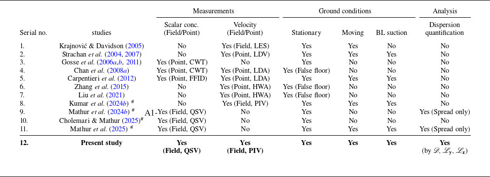
Comparison of existing literature on Ahmed body wake studies with the present work.

 $^\#$
Authors’ own publications.
LES, large-eddy simulation; CWT, cold-wire thermometry; FFID, fast-flame ionisation detector; QSV, quantitative smoke visualisation; LDV, laser Doppler velocimetry; LDA, laser Doppler anemometry; HWA, hot-wire anemometry; PIV, particle image velocimetry; BL, boundary layer.
Appropriate ground conditions are expected to be crucial in both computational fluid dynamics and wind tunnel simulations of moving vehicles, as the vehicle wake topology and particulate dispersion characteristics are likely to be significantly influenced by ground conditions. Please refer to table 1, which summarises and compares the existing literature of studies of vehicle wake discussed above. The available literature shows that only a limited number of studies have systematically investigated the wake flow topology and scalar dispersion under moving ground conditions. A key gap in the methodology exists because nearly all existing scalar dispersion experiments rely on intrusive point measurement techniques for concentration and dispersion. These methods not only carry the risk of flow disruption but are inherently incapable of capturing the instantaneous concentration patterns and dispersion necessary for analysis of pollutant transport. This highlights a critical need for research employing appropriate moving ground conditions and non-intrusive field measurements of concentration to accurately quantify dispersion in the vehicle wake. Although there were several reported velocity measurements for the Ahmed body wake with the stationary wind tunnel ground, they did not agree amongst themselves, specifically regarding the existence of a third spanwise vortex near the ground (discussed in detail in later sections). It is therefore useful to make velocity and concentration measurements within the same experimental set-up.
The present investigation directly addresses these research gaps by examining the influence of wind tunnel ground conditions on the flow topology and dispersion in the near wake of an Ahmed body with two rear slant angles (
 $\phi =25^{\circ }$
and
 $40^{\circ }$
). This study provides a comprehensive comparison of the flow topology and dispersion phenomena under both stationary and moving ground condition for the Galilean transformation, directly quantifying the importance of accurate ground conditions. We employ PIV and quantitative smoke visualisation (QSV) (Cholemari & Mathur Reference Cholemari and Mathur2025) to obtain the velocity and concentration fields in the Ahmed body near wake, under stationary and moving ground conditions, within the same experimental configuration, which has not been done previously. These measurements allow us to directly correlate the measured velocity and concentration fields to establish a link between wake flow structures and the resulting dispersion characteristics. Finally, we quantify the dispersion in the near wake using defined parameters, including the non-dimensional dispersion (
 $\mathscr{D}$
) and dispersion length scales (
 $\mathscr{L}_y,\;\mathscr{L}_z$
).
The remainder of this paper is structured as follows. Section 2 provides a detailed description of the experimental set-up (§ 2.1) and a brief discussion on the QSV technique (§ 2.2). Section 3 presents and analyses the results, highlighting the impact of ground conditions on the flow topology and scalar concentration in the wake. Section 3.3 discusses the quantification of dispersion and provides insights into the influence of wind tunnel ground conditions on dispersion. The findings from the present study are finally summarised in § 4.
2. Experimental procedure and details
2.1. Experimental set-up and vehicle model
A schematic of the environmental wind tunnel with rolling road. A side view of the schematic of the rolling road and boundary layer suction is also shown (at the bottom), along with their major components.

The experiments were conducted in an open-circuit, suction-type environmental wind tunnel with a test section of dimensions;
 $14\rm\,m\times 2\rm\,m\times 2\rm\,m$
. The glass wall on one side of the wind tunnel provides optical access. A schematic of the wind tunnel is shown in figure 3. The maximum turbulence intensity away from the wall boundary layer in the test section is approximately
 $1\,\%$
. A rolling road (Bhanu et al. Reference Bhanu, Mathur, Cholemari and Veeravalli2022, Reference Bhanu, Kumar, Cholemari and Veeravalli2024) (with moving ground of dimensions
 $1.6\rm\,m \times 0.88\rm\,m$
, made of an endless continuous belt) is used to provide moving ground conditions, to replicate actual road conditions. The rolling road belt can be made to move with the same velocity as that of the wind tunnel free stream (
 $U_{\infty }$
). A boundary layer suction system with a tangential suction slot (dimensions:
 $0.86\rm\,m\times 0.12\rm\,m$
) positioned just upstream of the rolling road was used to remove the oncoming boundary layer formed due to the stationary wind tunnel floor upstream of the rolling road. Before conducting the dispersion experiments, the performance of the rolling road and boundary layer suction was evaluated by performing boundary layer measurements, with and without operation of the rolling road and boundary layer suction system. Figure 4 shows the velocity profile (
 $u/U_\infty$
) measured at different downstream locations,
 $x/h$
(where
 $x$
is streamwise distance on the moving ground and
 $h$
is Ahmed body height) from the leading edge of the rolling road belt for both moving and stationary ground conditions in the empty test section. The
 $y$
axis of the plots are non-dimensionalised by the local boundary layer thickness (
 $\delta (x)$
) for the stationary ground case. These measurements were conducted to determine the boundary layer thickness (
 $\delta$
) in each (stationary/moving) case. The rolling road, along with the boundary layer suction, showed that a significant reduction in boundary layer thickness was obtained in the test section. The measurements show that the system reduces the boundary layer thickness by 57
 $\,\%$
–72
 $\,\%$
and the displacement and momentum thicknesses by more than
 $95\,\%$
, indicating that the system can avoid boundary layer formation. The rolling road system does not disturb the flow either mechanically or thermally. The mechanical vibrations of rolling road were measured using four piezoelectric accelerometers. Vibration measurements indicate that the dominant frequency and amplitude of vibration (
 $y_{max} = 4.26 \,\rm {\unicode{x03BC}} m$
) are insufficient to significantly affect the flow near the moving ground. Additionally the rise in the moving belt temperature due to the friction between the moving belt and the backing plate was measured (by thermal imaging camera) to be
 $\Delta T \approx 0.8\,\rm ^{\circ}C$
. This excess temperature induces an upward velocity of
 $0.5\,\rm cm\,s^{-1}$
through density changes. Therefore, the estimated disturbances due to this induced velocity is less than
 $0.16\,\%$
of the mean flow velocity, and hence the rolling road can simulate actual road conditions accurately in the wind tunnel. More importantly, the rolling road provides the moving ground condition required for the Galilean transformed flow. More information related to the design of the main components of the rolling road can be found in Bhanu et al. (Reference Bhanu, Mathur, Cholemari and Veeravalli2022, Reference Bhanu, Kumar, Cholemari and Veeravalli2024).
Comparison of the boundary layer velocity (
 $u/U_\infty$
) profile for stationary and moving ground case at streamwise distances,
 $x/h=0.61,\;1.22,\;1.83,\;3.05,\;4.27$
and
 $6.10$
away from the leading edge of the rolling road.

Dimensions (in mm) of the Ahmed body (used in the present study) with wheel and smoke source. The detachable rear end of the model is also shown.

Illustration of the experimental set-up for smoke concentration measurement. The rolling road and the boundary layer suction system are also shown.

The vehicle model used for this study is a
 $57\,\%$
scaled model of the Ahmed body. Two rear slant angles in high drag (
 $\phi = 25^\circ$
) and low drag (
 $\phi = 40^\circ$
) regimes (Zhang et al. Reference Zhang, Zhou and To2015; Liu et al. Reference Liu, Zhang, Zhang and Zhou2021) were used for the experiments. Figure 5 presents the schematic (with dimensions) of the Ahmed body and the interchangeable rear ends (corresponding to the two rear slant angles) used in the present study. To place the model on the moving ground, the four cylindrical struts (i.e. model legs) in the standard Ahmed body were replaced with wheels of
 $26\,\rm mm$
diameter. The vehicle model was held in place on the rolling road using thin stainless steel strings of
 $1.1\,\rm mm$
diameter attached at the four sides of the vehicle model, as shown in figure 5. The front end of the model was positioned
 $30\,\rm cm$
away from the leading edge of the rolling road. The blockage ratio for the vehicle model is 0.9
 $\,\%$
. The velocity and concentration measurements were conducted at a Reynolds number;
 $\textit{Re}_l=1.21 \times 10^5$
,
 $\textit{Re}_h=0.33 \times 10^5$
with a free-stream velocity of
 $U_{\infty }=3\,\rm m\,s^{-1}$
.
Figure 6 illustrates the schematic representation of the experimental set-up for the dispersion experiments. The diagram shows the Ahmed body placed on the rolling road moving belt within the test section, the boundary layer suction system is also shown, which is connected to the axial blower for the boundary layer suction. A source pipe with a diameter of
 $d_s=1.6\,\rm cm$
was installed at an offset location (
 $x^* = 0, \; y^* = 0.12$
and
 $z^* = -0.31$
) of the rear vertical base of the Ahmed body. The coordinate system used in this study is shown in figures 5 and 6. The origin
 $O$
was taken at the rear vertical of the model vehicle, on the centreline of the moving ground in the wind tunnel. The
 $x^*,\;y^*$
and
 $z^*$
coordinates represent the streamwise, vertical and cross-stream directions in the wind tunnel, defined as
 \begin{equation} x^* = \frac {x}{h}, \,\,\,\,\ y^* = \frac {y}{h}, \,\,\,\,\ z^* = \frac {z}{h}, \end{equation}
where
 $h$
is the height of the Ahmed body. Ethylene-glycol smoke particles of diameter
 $\approx$
1
 $\,\rm {\unicode{x03BC}} m$
were released through the source pipe, by using a
 $1200\,\rm W$
smoke machine, which is kept inside the Ahmed body, as shown in figure 6. The smoke particles released in the flow are essentially passive scalars. To evaluate this, we calculate the particle Stokes number (
 $\textit{St}_{\!p}$
), defined as the ratio of the relaxation time of the particle (
 $\tau _p$
) to the characteristic time scale of the flow (
 $\tau _{\textit{flo}w}$
)
 \begin{equation} \textit{St}_{\!p}=\frac {\tau _p}{\tau _{\textit{flo}w}}, \end{equation}
 \begin{equation} \textit{St}_{\!p}=\frac {\rho _p\;d_p^2\;U_\infty }{18\;\rho _{\textit{air}}\;\nu \;h}=5.87\times 10^{-5}, \end{equation}
where
 $\rho _p$
is smoke particle density,
 $\rho _{\textit{air}}$
is the density of air (
 $\rho _p/\rho _{\textit{air}}=1153.50$
) and
 $\nu$
is the kinematic viscosity of the air. The characteristic time scale of the flow is defined by
 $\tau _{\textit{flo}w}=h/U_\infty$
(where
 $h$
is the Ahmed body height and
 $U_{\infty }$
is the free-stream velocity). The smoke particles have a particle Stokes number (
 $\textit{St}_{\!p}$
) far less than unity (
 $\textit{St}_{\!p}=5.87\times 10^{-5}$
), and for
 $\textit{St}_{\!p}\lt \lt 1$
, particles follow fluid streamlines closely with negligible slip between particle and fluid. The displacement lag between fluid and smoke particle is of the order
 $\tau _p\times \Delta U\approx 11.1\,\rm {\unicode{x03BC}} m$
, which is much smaller than the smallest scale that can be resolved by the measurement system, i.e.
 $0.43\,\rm mm$
(which is the spatial resolution of the camera in the current experimental set-up,
 $0.43\times 0.43\,\rm mm^2\,pixel^{-1}$
). For the illumination of smoke particles, a continuous beam solid-state laser (MGL-W532,
 $5000\,\rm mW$
,
 $\lambda _{\textit{laser}}$
=
 $532\,\rm nm$
) was used; the laser beam was directed to a plano-concave cylindrical lens (focal length
 $-25\,\rm mm$
) that creates a laser sheet (
 $2\,\rm mm$
in thickness) in
 $y{-}z$
plane. The laser-illuminated smoke particles scatter the light, which was captured by a DSLR camera (Canon EOS-90D). The camera captured instantaneous images at a frame rate of 50 f.p.s. with a resolution of
 $1920 \times 1080$
pixels. The camera settings include an aperture of
 $f/5.6$
and an exposure time of
 $1.25\times 10^{-3} \,\rm s$
. The camera was positioned
 $5m\approx 30h$
downstream of the Ahmed body, as shown in figure 6. The concentration measurements were taken at six downstream locations behind the Ahmed body, at
 $x^* = 0.25$
,
 $0.5$
,
 $1$
,
 $1.5$
,
 $2$
and
 $2.5$
, under both moving and stationary ground conditions.
Schematic view showing the QSV technique used for the concentration measurements.

2.2. Concentration measurement technique
The quantitative smoke visualisation technique is used for scalar concentration field measurement in this study. A brief introduction to the technique is given in this section. A detailed discussion on the QSV technique is given in Cholemari & Mathur (Reference Cholemari and Mathur2025). The flow is seeded with fine smoke particles, and a thin laser sheet is used to illuminate the smoke. The illuminated smoke particles scatter the incident laser within the Mie-scattering range, as
 $d_p\geqslant \lambda _{\textit{laser}}$
Bohren & Huffman (Reference Bohren and Huffman2008) (where
 $d_p$
is the diameter of smoke particles and
 $\lambda _{\textit{laser}}$
is the wavelength of the laser illuminating the smoke particles). The scattered light is captured by the camera placed orthogonally to the laser sheet downstream of the measurement plane (refer to figure 7). The concentration regime is so chosen such that the intensity of the scattered light (
 $S$
) is proportional to the intensity of the incident laser (
 $I$
) and the concentration of the smoke (
 $C$
) locally
 \begin{equation} S \propto I C. \end{equation}
The laser illumination intensity
 $I$
is spatially varying. The linear relationship between concentration
 $C$
and signal intensity
 $S$
is established by using a calibration procedure (discussed in § 2.2.1). The images of the smoke-laden flow are processed to get the smoke concentration field in the measurement planes. The technique also implements an iterative attenuation correction based on the Beer–Lambert law, to correct for laser intensity attenuation using mean concentration fields as calibration fields (Cholemari, Vishnubhatla & Krishnan Reference Cholemari, Vishnubhatla and Krishnan2024; Cholemari & Vishnubhatla Reference Cholemari and Vishnubhatla2024). This enhances the accuracy beyond what is achievable by a pixel-wise calibration using a uniform concentration field (Crimaldi Reference Crimaldi2008). A projective transformation is done on raw images before the concentration evaluation to account for the effects of laser sheet widening (sheet thickness perpendicular to the image remains constant). The use of a reference concentration is also not required for attenuation correction. A background image is subtracted prior to processing to account for the background noise at each pixel. More details about the QSV technique and its implementation are given in Cholemari & Mathur (Reference Cholemari and Mathur2025).
2.2.1. Calibration for concentration measurements
Illustration of the experimental set-up for the calibration.

Prior to experimental measurements, a calibration process was conducted to establish a relationship between the smoke concentration (
 $C$
) in the wake and the intensity of light scattered (
 $S$
) by these particles (detailed calibration procedure is given in Cholemari & Mathur Reference Cholemari and Mathur2025). The calibration experiments were conducted using the set-up illustrated in figure 8. The smoke was released into a mixing duct made of PVC with a diameter of
 $d_{md}=10.16\,\rm cm$
and a length of
 $1\,\rm m$
, positioned at the centre of the wind tunnel test section. A
 $1200\,\rm W$
smoke machine is used to release the smoke. The smoke machine is kept perpendicular to the mixing duct, well away from the mixing duct entrance, and a metal bent pipe is connected to the smoke machine, which allows the smoke to come out at the centre (along the axis) of the mixing duct (please refer to figure 8). The smoke is mixed with the free-stream flow (free-stream velocity,
 $U_{\infty }=3\,\rm ms^{-1}$
) in the mixing duct, producing uniformly mixed smoke at the exit of the mixing duct. The uniformly mixed smoke particles are illuminated with the help of a continuous wave laser (MGL-W532) just outside the duct by a planar laser sheet (in the cross-stream plane, i.e. the
 $y{-}z$
plane) obtained from sheet optics (plano-concave cylindrical lens,
 $f=-25\,\rm mm$
). The smoke particles illuminated by the laser sheet scatter the light, which is captured by a DSLR camera (Canon EOS 90D) placed at a downstream location. The instantaneous images (approximately
 $2000$
frames) captured by the camera were processed in MATLAB to obtain a time-averaged image. The time-averaged image represents the signal intensity for the corresponding uniform concentration of smoke released in the flow. The smoke machine is connected to an electric voltage regulator (silicon controlled rectifier triac type) to control the smoke thickness by adjusting its input power, thereby achieving different levels of smoke concentration. The relationship between the smoke concentration (
 $C$
) and the signal intensity (
 $S$
) is determined by conducting experiments at different concentration levels. The attenuation of laser intensity and the geometry of the laser sheet are also accounted for during the calibration process. The volumetric flow rate (
 $Q_{\!f}$
) of the smoke liquid is measured to determine the absolute concentration of smoke released. The concentration of smoke (in ppmw) defined based on the flow rate is given below as
 \begin{equation} \bar {C}=\frac {\rho _{\textit{fog}} Q_{\!f}}{\rho _{\textit{air}}A\bar {U}_{\!md}}\times 10^6, \end{equation}
where the
 $\bar {(\;\boldsymbol{\cdot }\;)}$
represents the spatial average over the mixing duct cross-section area,
 $A$
is the area of dilution,
 $\rho _{\textit{fog}}$
is the density of the smoke liquid (
 $1300\,\rm kg\,m^{-3}$
),
 $\rho _{\textit{air}}$
is the density of air (
 $1.225\,\rm kg\,m^{-3}$
) and
 $\bar {U}_{md}$
is the average/bulk velocity of the flow through the mixing duct. The average velocity of the flow through the mixing duct is determined by performing PIV measurements in the longitudinal (
 $x{-}z$
) plane passing through the axis of the mixing duct. The reference concentration released from the mixing duct can be defined as
 \begin{equation} \bar {C}=\frac {4\rho _{\textit{fog}} Q_{\!f}}{\rho _{\textit{air}} \pi d_{md}^2U_\infty }\times 10^6, \end{equation}
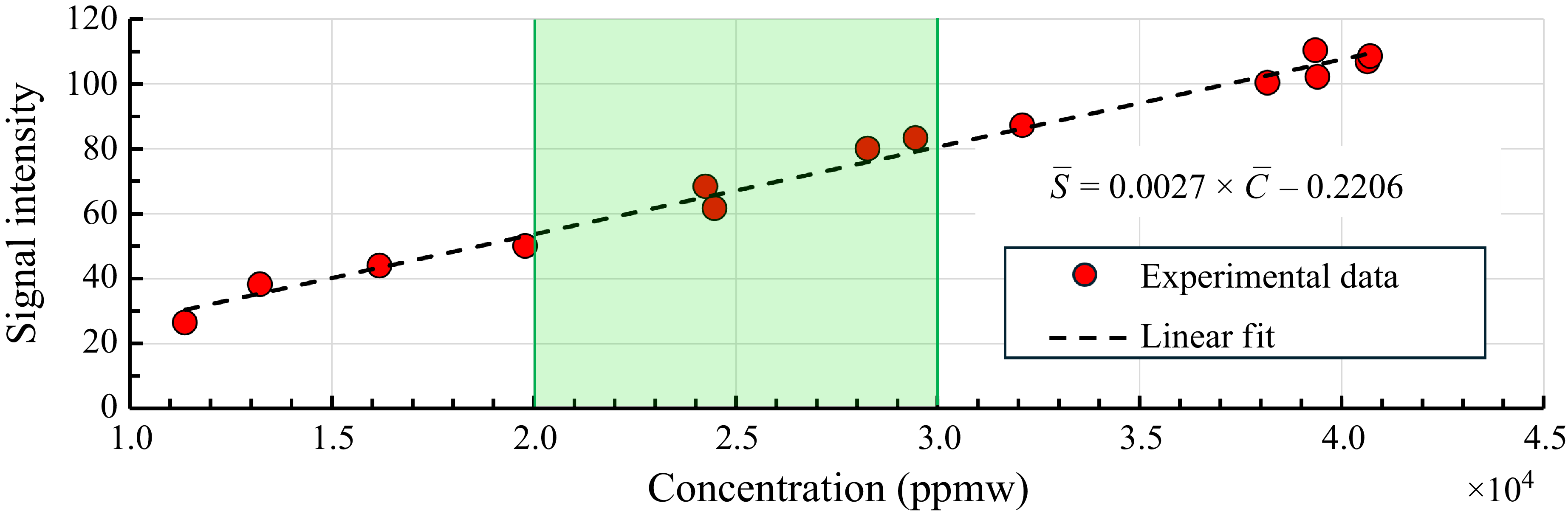
Calibration curve showing the relationship between signal intensity (
 $\bar {S}$
) and smoke concentration (
 $\bar {C}$
). The black dashed line is the linear fit to the experimental data. The green region shows the concentration range in which all the dispersion experiments were performed.

where
 $d_{md}$
is the diameter of the mixing duct. Here,
 $\bar {C}=C_{\textit{ref}}$
is the uniform concentration released from the mixing duct.
Figure 9 shows the calibration results. The results illustrate a good linear response between signal intensity (
 $\bar {S}$
) and smoke concentration (
 $\bar {C}$
). The linear region is evident in the trend for concentrations between
 $10\,000 \leqslant \bar {C} \leqslant 40\,000$
ppmw. A linear fit to the data in the given regime gives the following relation:
 \begin{equation} \bar {S} = 0.0027 \times \bar {C} -0.2206, \end{equation}
where
 $\bar {S}$
is the signal intensity, and
 $\bar {C}$
is the smoke concentration (units of
 $\bar {C}$
are in ppmw). Equation (2.8), derived from (2.7), is used to get the smoke concentrations from the signal intensity obtained in the dispersion experiment as follows:
 \begin{equation} \bar {C} = 370.37 \times \bar {S} + 81.70. \end{equation}
Equation (2.8) implies that less than
 $0.4\,\%$
of the error due to background noise remains when compared with the mean concentration. All the dispersion experiments were performed in the concentration range
 $20\,000\leqslant \bar {C}\leqslant 30\,000$
(ppmw) (shown by the green region in figure 9), entirely in the linear range.
2.3. Experimental set-up for particle image velocimetry
Schematic of the PIV set-up for velocity measurements in the model midplane. The coordinate origin is defined at the ground level at the model midplane.

Particle image velocimetry was employed to measure the velocity field in the near wake of the Ahmed body for both ground conditions. The flow was seeded with ethylene-glycol particles with a diameter
 ${\approx}1\,\rm {\unicode{x03BC}} m$
, generated by a smoke machine (
 $1200\,\rm W$
). The PIV experiments were conducted in the wind tunnel described in § 2.1. The free-stream velocity was
 $U_\infty =3\,\rm m\,s^{-1}$
(same as for the dispersion experiments), corresponding to
 $\textit{Re}_l=1.21\times 10^5$
. Velocity measurements were performed at the midplane (i.e.
 $x{-}y$
plane at
 $z^*=0$
) of the Ahmed body, as illustrated in figure 10. The flow field was illuminated using an MGL-W532 continuous wave, solid-state laser (
 $\lambda _{\textit{laser}} = 532\,\rm nm$
). The laser beam was passed through a plano-concave lens (
 $f=-25\,\rm mm$
) to obtain a
 $2\,\rm mm$
thick laser sheet, which illuminated the midplane behind the model. A Canon EOS 90D DSLR camera (CMOS sensor
 $22.3\,\rm mm\times 14.9\,\rm mm$
), positioned perpendicular to the laser sheet outside the wind tunnel, captured the images through the optical window at a resolution of
 $1920 \times 1080$
pixels with a frame rate of
 $100$
f.p.s. and an exposure time of
 $6.4\times 10^{-4}$
s. The magnification factor of the captured images was
 $217\,\rm {\unicode{x03BC}} m\,\text{pixel}^{-1}$
, yielding a field of view of
 $410 \times 246\,\rm mm^2$
(
 $2.5\,h\times 1.4\,h$
). To obtain the average flow characteristics, between
 $2000$
and
 $3000$
image pairs were recorded for each case. The PIV images were processed using an in-house PIV code (Cholemari Reference Cholemari2007) to estimate the two components of velocity in the image plane. It is a multi-grid, multi-pass, fast Fourier transform based cross-correlation algorithm with window deformation and shifting. Three passes were used, first pass operates on a large interrogation window (
 $96\times 96$
pixels), the subsequent passes operate on smaller interrogation windows (
 $32\times 32$
pixels) with
 $50\,\%$
overlap. A total of
 $65\times 119$
in-plane instantaneous vectors were obtained in the region of interest.
The PIV image parameters were set up to minimise the errors, as given below. The effective particle diameter (
 $d_e$
) is given by
 \begin{equation} d_e=\sqrt {(d_s^2+M^2d_p^2)}, \end{equation}
with
 \begin{equation} d_s =2.44 (1+M) (f/D) \lambda , \end{equation}
where
 $d_s$
is the diffraction limited particle size,
 $M$
is the image magnification,
 $d_p$
is the particle size and
 $f/D$
is the f-stop number of the camera. For the present measurement configuration the effective particle diameter is calculated to be
 $d_e =7.36\,\rm {\unicode{x03BC}} m$
, which is 2.3 pixels, close to the optimal size of 2 pixels (Westerweel Reference Westerweel1997). Also, the recommended displacement is kept at approximately 1/4th of the interrogation window for minimum error (e.g. Prasad Reference Prasad2000). These choices minimise the random errors. The recording rate is
 $100\,\rm Hz$
with a shutter of 1/1600 s. The maximum displacements are approximately 12 pixels with a streaking of less than 0.7 pixels. This adds to the root-mean-squared (r.m.s.) error by widening the particle image to 3 pixels in the worst case. This makes the particle image size slightly sub-optimal in some locations. We therefore conservatively estimate the measurements to be of adequate standard with a worst r.m.s. error of approximately 0.05 pixels, which translates to a random error of approximately 0.5 % of the mean flow magnitude. The peak-locking bias error is corrected using the approach given in Cholemari (Reference Cholemari2007). We estimate the peak-locking error to be 0.02 pixels at worst, corrected to better than 0.002 pixels, and thus does not affect the statistics considered in the present analysis significantly. Please note that, in this set of experiments, due to hardware limitations, simultaneous measurements of velocity and concentration could not be done. In case of measurements in the rear vertical planes, the out of plane motion of the smoke was too large between frames for an accurate PIV measurement. However, this is not a limitation for QSV measurements, which rely on images from individual frames. In case of midplane measurements, while the PIV measurements were satisfactory, accurate attenuation correction could not be made for QSV measurements as the path of the laser sheet could not be visualised in its entirety and also the laser sheet itself was not parallel, to add to the inaccuracy. However, for the purposes of analysis conducted in this paper, the measurements are adequate.
3. Results and discussion
This section presents and discusses the results obtained from the PIV and QSV experiments. Section 3.1 includes a discussion and analysis of the spanwise flow structures obtained from the PIV measurements. In all cases, we also compare the flow structures obtained with a fixed ground. Time-averaged velocity fields, streamline patterns and vorticity contours are presented and discussed. These measurements provide insights into the behaviour of smoke and its dispersion within the recirculation region. An effort is made to find the relation between turbulent structures and smoke dispersion to understand how turbulent structures influence dispersion in the wake. Following this, § 3.2 presents the concentration measurements obtained from the QSV technique. Finally, in § 3.3, the dispersion in the near wake is quantified, and the dispersion parameters are estimated using the quantitative concentration measurements and observed dispersion patterns.
3.1. Particle image velocimetry results: spanwise flow structures in the near wake
Particle image velocimetry measured time-averaged velocity field in the model midplane, behind the Ahmed body with rear slant angles of (a–b)
 $\phi =25^\circ$
and (c–d)
 $40^\circ$
for both stationary and moving ground conditions. Flow is from left to right.

This section discusses the spanwise flow structures in the near wake of the Ahmed body, highlighting the effects of the wind tunnel ground conditions on the mean flow characteristics for both rear slant angles (
 $\phi =25^\circ,\;40^\circ$
) of the Ahmed body. Figure 11 presents a comparison of time-averaged velocity vectors (in the model midplane
 $z^*=0$
) in the near wake of the Ahmed body with rear slant angles
 $\phi =25^\circ$
(figure 11
a,b) and
 $\phi =40^\circ$
(figure 11
c,d), for both stationary and moving ground conditions. The velocity vectors show the formation of spanwise flow structures in the near wake of the Ahmed body. The near wake is characterised by two counter-rotating vortices, the upper one (vortex A) in a clockwise direction and the lower one (vortex B) in an anticlockwise direction inside the separation bubble. The system of vortices observed in the present study (for both the rear slant angles) is in agreement with the earlier observations by Ahmed et al. (Reference Ahmed, Ramm and Faltin1984), Lienhart & Becker (Reference Lienhart and Becker2003), Wang et al. (Reference Wang, Zhou, Pin and Chan2013), Zhang et al. (Reference Zhang, Zhou and To2015) and Liu et al. (Reference Liu, Zhang, Zhang and Zhou2021). These vortices are also schematically shown in figure 1. The direction and size of the vortices are shown in the figure; the size and position of these vortices vary depending on the rear slant angle and wind tunnel ground conditions, as shown in figure 11. The flow around the Ahmed body with rear slant angle
 $\phi =25^\circ$
remains attached to the rear slant surface for both stationary and moving ground conditions. The flow coming over the rear slant and underbody of the model separates at the upper and lower edges of the rear vertical, respectively, to form the spanwise vortices A and B (refer to figure 11
a,b). At
 $\phi =40^\circ$
, the flow separates at the leading edge of the rear slant. This massive flow separation causes a significantly bigger upper vortex (vortex A), an extended recirculation region and backflow over the rear slant (refer to figure 11
c,d). Figure 11 indicates that the flow topology in the near wake is significantly affected by the wind tunnel ground conditions. The spanwise vortices A and B are seen to be moving toward the ground and are being stretched in the streamwise direction (compare figure 11
a with 11
b and figure 11
c with 11
d). In addition to the spanwise counter-rotating vortices (vortices A and B), a third clockwise vortex was also observed close to the ground (hence the name ‘ground vortex’ and it is referred to as ‘vortex G’) for the stationary ground condition (refer to figures 11
a and 11
c). However, for moving ground conditions, this additional ground vortex is not present (see figures 11
b and 11
d). Please note, as the PIV images are taken at
 $100\,\rm Hz$
, the typical data duration is
 $20-30\,\rm s$
continuously sampled. Even in the slow moving wake, with the typical velocity being around
 $50 \,\rm cm\,s^{-1}$
, at least 4 large-scale structures are swept away every second. Hence, the averaging, in the worst case, is over 80 largest-scale structures and progressively over larger and larger lengths of independent data as the scales become smaller. Naturally, the situation improves at locations where the velocity is larger. Hence, we believe that the PIV data are of adequate duration for the convergence of spatial statistics, and to confidently detect the presence of flow structures such as this vortex (vortex G). Thus vortex G is not an artefact of limited sample size or the lack of accuracy in the PIV measurements.
The existence of the ground vortex (vortex G) in the stationary ground conditions can be attributed to the presence of the boundary layer on the stationary wind tunnel floor, and the shear present therein. Basically, the existence of the ground vortex (vortex G) depends on the balance of momentum coming out of the ground clearance below the Ahmed body and its attenuation by the ground, and the input momentum from the flow above the shear layer detaching from the rear slant of the Ahmed body. The ground vortex does not exist in the moving ground case, because the attenuation of the momentum due to shear at the ground is absent. The decelerated flow in the boundary layer, in the case of a stationary floor, leads to the formation of this additional vortex. Earlier studies (Venning et al. Reference Venning, Lo Jacono, Burton, Thompson and Sheridan2015; Kumar et al. Reference Kumar, Cholemari and Veeravalli2024b
) have documented a similar third vortex formation near the ground in the wake of the vehicle model for the stationary ground condition. The balance of momentum can be significantly influenced by various geometrical (e.g. ground clearance, aspect ratio and rear slant angle of the Ahmed body) and flow parameters (free-stream velocity, boundary layer thickness) that decide the existence of vortex G. It is observed that the massive separation on the rear slant behind the
 $\phi =40^\circ$
model leads to significant deceleration of the flow coming from the top of the model and hence the vortex G formed behind
 $\phi =40^\circ$
model is larger compared with the
 $\phi =25^\circ$
model (see figures 12
a and 12
c). The moving ground enhances the underbody flow, which also results in an extended recirculation region for both rear slant angles (see figures 11
b and 11
d).
Particle image velocimetry measured time-averaged streamlines in the model midplane, behind the Ahmed body with rear slant angles of (a–b)
 $\phi =25^\circ$
and (c–d)
 $\phi =40^\circ$
for both stationary and moving ground conditions. Flow is from left to right.

Figure 12 presents the time-averaged streamlines obtained from PIV measurements in the near wake of the Ahmed body with rear slant angles of
 $\phi =25^\circ$
and
 $\phi =40^\circ$
, under both stationary and moving ground conditions. The streamlines show the system of spanwise vortices in the recirculation region. For
 $\phi =25^\circ$
, the streamlines in figures 12(a) and 12(b) indicate that the flow remains attached to the rear slant surface, with a strong downwash, limiting the size of the recirculation region. In contrast, for
 $\phi =40^\circ$
, the flow detaches at the leading edge of the rear slant; forming a larger separation bubble spanning both rear slant and rear vertical. This results in a significantly larger upper recirculation vortex A. Additionally, the streamlines show the size of the ground vortex (vortex G) observed in the stationary ground conditions. Clearly, vortex G is larger behind the
 $\phi =40^\circ$
model than behind the
 $\phi =25^\circ$
model, which can be attributed to the massive flow separation at
 $\phi =40^\circ$
. The flow separation further promotes flow retardation and hence the formation of vortex G, leading to a bigger vortex G behind the
 $\phi =40^\circ$
model. The different wake topologies observed for different ground conditions and rear slant angles are expected to have a significant impact on pollutant dispersion in the near wake.
3.1.1. Critical flow points
To analyse the effects of wind tunnel ground conditions on spanwise flow structures, three critical flow points are identified in the wake. Specifically, they are focus point 1 (
 $F_1$
), located at the centre of the upper vortex (vortex A); focus point 2 (
 $F_2$
), located at the centre of the lower vortex (vortex B); and the saddle point (SP). The positions of
 $F_1$
and
 $F_2$
(in terms of
 $x^*, \;y^*$
) are determined from time-averaged streamlines (as shown in figure 12). Figure 13 presents the location of critical flow points in the model midplane under stationary and moving ground conditions for both the rear slant angles. This provides a quantitative and visual representation of the impact of wind tunnel ground conditions on the spanwise wake flow structures for both the rear slant angles of the Ahmed body. The figure indicates that varying the rear slant angle from
 $25^\circ$
to
 $40^\circ$
has a significant influence on the positions of critical flow points. Notably, the vertical position and the horizontal positions of
 $F_1,\,F_2$
and SP (compare figure 13
a,b). For both the rear slant angles, the critical points exhibit significant shifts under different wind tunnel ground conditions. In the moving ground condition, the absence of the ground vortex (vortex G) leads to a lower vertical position of all the critical points compared with the stationary condition. Furthermore, the enhanced underbody flow due to the moving ground causes the critical points to shift in the streamwise direction from the Ahmed body rear vertical, resulting in a longer recirculation region. This significant variation in wake flow topology, as shown by movements in the critical flow points, due to different ground conditions, considerably affects the dispersion in the near wake. This will be presented and discussed in § 3.2 with the concentration measurements results.
Locations of critical flow points (
 $F_1,\;F_2$
and SP) in the near wake of the Ahmed body with rear slant angles (a)
 $\phi =25^\circ$
and (b)
 $\phi =40^\circ$
for stationary (St) and moving (Mv) ground conditions.

3.1.2. Recirculation region
The time-averaged streamlines presented in figure 12 were used to determine the extent of the recirculation region in the near wake. The recirculation region is characterised by negative streamwise velocity components in the wake. The recirculation region consists of a system of spanwise vortices that are responsible for the mixing of smoke in this region, making this region particularly important in the context of pollutant dispersion studies. These spanwise vortices are also responsible for entrainment and mixing of the particulate matter present on the ground; therefore, the recirculation region is also referred to as the pickup region (Richards et al. Reference Richards, Wright, Baker and Baxendale2002). The size or recirculation region is quantified by the recirculation length, which is defined as the maximum streamwise distance (
 $x^*$
) from the model rear vertical, where the time-averaged streamwise velocity component becomes zero (i.e.
 $\langle U\rangle =0$
) and is defined as
 \begin{equation} L^*_R= \textit{max}(x^*)\vert _{\langle U\rangle =0}. \end{equation}
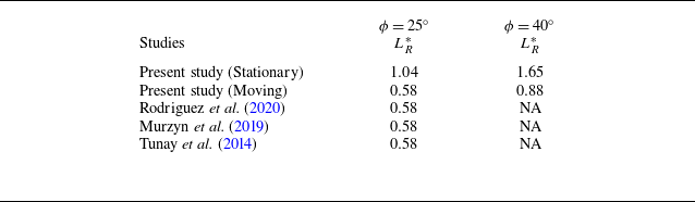
Table 2 presents the calculated recirculation lengths for the Ahmed body with both stationary and moving ground conditions. From the table, it is clear that the rear slant angle and the ground conditions significantly affect the recirculation length (
 $L^*_R$
). As observed in figure 12, flow separation at the leading edge of the rear slant for
 $\phi =40^\circ$
results in a significantly larger recirculation region compared with the
 $\phi =25^\circ$
case. Furthermore, the presence of the clockwise ground vortex (vortex G) in the recirculation region for stationary ground conditions significantly increases the recirculation length for both rear slant angles. The enlargement in the recirculation region is shown by the increase in the values of
 $L^*_R$
, see table 2.
Comparison of recirculation length (
 $L^*_R$
) for both ground conditions.

Iso-contours of time-averaged spanwise vorticity
 $\langle \omega _z\rangle$
in the model midplane plane
 $z^*=0$
behind the Ahmed body with slant angles of (a–b)
 $\phi =25^\circ$
and (c–d)
 $\phi =40^\circ$
for both stationary and moving ground conditions. Contour cutoff levels are
 $\langle \omega _z\rangle = \pm 0.25\rm \,s^{-1}$
.

Figure 14 illustrates time-averaged spanwise vorticity (
 $-\langle \omega _z \rangle$
) iso-contours in the near wake of the Ahmed body for both stationary and moving ground conditions. Positive (anticlockwise) vortices are depicted with dashed red lines, while negative (clockwise) vortices are represented by solid blue lines. A pair of counter-rotating recirculation vortices (vortices A and B) is evident in all cases in the figures. For the
 $\phi =25^\circ$
model, a strong downwash on the rear slant suppresses the flow separation, resulting in vorticity contours that remain attached to the slant (figures 14
a and 14
b). The interaction of spanwise vortices near the rear vertical leads to the formation of smaller regions of positive (
 $+\langle \omega _z \rangle$
) and negative (
 $-\langle \omega _z \rangle$
) vorticity, at the models' rear vertical. In contrast, for the
 $\phi =40^\circ$
model, the vorticity contours are completely detached from the rear slant (see figures 14
b and 14
d). The flow separation at the leading edge of the rear slant causes significant flow reversal. This flow reversal also contributes to the formation of small regions of positive
 $+\langle \omega _z \rangle$
(anticlockwise vorticity) attached to the rear slant. In the moving ground conditions (refer to figure 14
b,d), the vorticity contours are observed to be stretched in the streamwise direction, as also seen in the movement of critical points (in figure 13). The observed streamwise stretching of vorticity contours under the moving ground (see figures 14
b and 14
d) shows the wake elongation that was inferred from the movements of critical points in figure 13. Additionally, the stronger vorticity for the stationary ground case near the ground indicates a greater level of shear and hence a greater degree of smoke transport is expected. This will be shown in the estimates of the dispersion in § 3.3
3.2. Concentration field measurements
Instantaneous images of the smoke at the downstream location
 $x^*=0.25$
in the near wake of the Ahmed body with slant angles (a–b)
 $\phi =25^\circ$
and (c–d)
 $40^\circ$
in the wind tunnel with the stationary and moving ground conditions.

Time-averaged image of the smoke at the downstream location
 $x^*=0.25$
in the near wake of the Ahmed body with slant angles (a–b)
 $\phi =25^\circ$
and (c–d)
 $\phi =40^\circ$
in the wind tunnel with the stationary and moving ground conditions.

Non-dimensional mean concentration
 $\langle C^*(y, z) \rangle$
contour in the near wake of Ahmed body (in cross-stream
 $y{-}z$
plane) with rear slant angle
 $\phi =25^\circ$
for stationary and moving ground conditions at downstream locations;
 $x^*=0.25, 0.5, 1$
and
 $ 1.5$
. The outlines of Ahmed body and the smoke source are also shown.

Non-dimensional mean concentration
 $\langle C^*(y, z) \rangle$
contour in the near wake of Ahmed body (in cross-stream
 $y{-}z$
plane) with rear slant angle
 $\phi =40^\circ$
for stationary and moving ground conditions at downstream locations;
 $x^*=0.25, 0.5, 1$
and
 $ 1.5$
. The outlines of Ahmed body and the smoke source are also shown.

This section presents and discusses experimental measurements of smoke concentration in the wake of the Ahmed body (
 $\phi =25^\circ$
and
 $40^\circ$
) for both stationary and moving ground conditions. Measurements were conducted at various cross-stream planes located at
 $x^*=0.25, \;0.5,\;1,\;1.5,\;2$
and
 $2.5$
. Figure 15 presents the instantaneous images of smoke at
 $x^*=0.25$
in the wake of the Ahmed body with slant angles
 $\phi =25^\circ$
and
 $\phi =40^\circ$
under the stationary and moving ground conditions. Behind the
 $\phi =25^\circ$
model, the presence of trailing vortices can be seen in the instantaneous image shown in figure 15(a,b). The sequence of the instantaneous images (captured with a time interval,
 $\Delta \;t=20\times 10^{-3}\,\rm s$
) shows the direction of the trailing vortices, indicated by the arrows. These trailing vortices create a downwash at the midplane, which carries smoke with it, thereby restricting the vertical dispersion at the midplane. Whereas, when
 $\phi =40^\circ$
, the trailing vortices do not exist, and a uniform mixing of smoke is seen (figure 15
c,d). The instantaneous images were processed in MATLAB to obtain the time-averaged (mean) image, which is a measure of the mean dispersion of smoke at a given location in the near wake. Any constant or static illuminated background and possible laser reflections were subtracted from the time-averaged image. Figure 16 shows the time-averaged images obtained in the cross-stream plane at the downstream location of
 $x^*= 0.25$
with the stationary and moving ground conditions. These images were further processed (as given in § 2.2) to obtain the concentration fields. The time averaging of the instantaneous concentration at a point (
 $C(y,z,t)$
) obtained from the instantaneous images (figure 15) is performed for
 $N$
images, where
 $N$
is between
 $ 1500 \text{ and } 2000$
. This is equivalent to obtaining the time-averaged (mean) concentration from the time-averaged image (e.g. figure 16).
The non-dimensional mean concentration is defined by
 \begin{equation} \langle C^*(y,z)\rangle = \frac {\langle C(y,z)\rangle }{C_{\textit{ref}}} . \end{equation}
The mean
 $\langle C(y,z)\rangle$
and instantaneous
 $C(y,z,t)$
concentrations are non-dimensionalised by the reference concentration
 $C_{\textit{ref}}=\bar {C}$
(defined by (2.6)) released from the source during experiments. The reference concentration (
 $C_{\textit{ref}}$
) was maintained constant during all the experiments. The non-dimensional concentration fields behind the Ahmed body at downstream locations,
 $x^*= 0.25, \;0.5,\; 1$
and
 $1.5$
with stationary and moving ground conditions are shown in figure 17 (
 $\phi =25^\circ$
) and in figure 18 (
 $\phi =40^\circ$
). The figures also show outlines of the Ahmed body and the smoke source. The impact of the wind tunnel ground conditions on the smoke dispersion can be observed from figures 17 and 18. The concentration fields obtained for stationary and moving ground conditions are observed to be significantly different; particularly, the dispersion patterns obtained for both ground conditions are different. In moving ground conditions, the concentration distribution shows that the smoke is more concentrated toward the ground, and the dispersion patterns are observed to shift toward the moving ground. This was also observed by Mathur et al. (Reference Mathur, Bhanu, Cholemari and Veeravalli2025) for the Ahmed body with
 $\phi =25^\circ$
. However, this observation is now found to be consistent for both of the rear slant angles (
 $\phi =25^\circ,\;40^\circ$
) of the Ahmed body (refer to figure 17, 18). The present results show that, regardless of the rear slant angle of Ahmed body, the ground condition affects the particle dispersion in a similar manner for both the subcritical (
 $\phi \lt \phi _c$
) and supercritical (
 $\phi \gt \phi _c$
) regimes. It can be observed that the vertical dispersion of the smoke is less in moving ground conditions than in stationary ground conditions (compare stationary and moving ground results in figure 17, 18). This will also be shown by the dispersion parameters presented in figure 22, in § 3.3.2. The formation of vortex G, as discussed in § 3.1, enhances the mixing of the smoke preferentially in the vertical direction (due to its spanwise orientation). This ground vortex (vortex G) is not present in the moving ground condition, as also shown by the movement of critical points (
 $F_1,\; F_2$
, SP) between both ground conditions (refer to figure 13). The flow structures (system of spanwise vortices, vortices A and B) move towards the ground and forward in a streamwise direction for moving ground conditions. Since the turbulent structures (which mix the smoke by entrapping the smoke) are moving towards the ground, it was expected that the concentration distribution would also be shifted downwards for the moving ground condition, and this is observed clearly in the concentration fields obtained for the moving ground condition. At
 $x^*=0.25$
, the dispersion extends up to
 $y^*=0.92$
and
 $y^*=1.41$
in the vertical direction behind the model with slant angles
 $\phi =25^\circ$
and
 $\phi =40^\circ$
, respectively, for the stationary ground case, whereas it is only
 $y^*=0.78$
and
 $y^*=1.03$
in the case of moving ground conditions. At
 $x^*=1$
, the dispersion contours extend up to
 $y^*=0.93$
and
 $y^*=1.11$
for the stationary ground case for
 $\phi =25^\circ$
and
 $\phi =40^\circ$
models, respectively, and
 $y^*=0.63$
and
 $y^*=0.82$
for the moving ground case in the model midplane,
 $z^*=0$
(see figure 17, 18). As also observed in previous studies (Gosse et al. Reference Gosse, Paranthoën, Patte-Rouland and Gonzalez2006a
,Reference Gosse, Patte-Rouland, Gonzalez and Paranthoën
b
; Keita Reference Keita2018), the smoke/scalar concentration decreases with the streamwise direction (
 $x^*$
), and a similar trend is observed in both the ground conditions and rear slant angles. The dispersion patterns also show that, in contrast to the dispersion in the vertical direction, the dispersion in the lateral direction is almost the same for both ground conditions at any given downstream location and slant angle. This behaviour of the dispersion patterns can be attributed to the spanwise nature of the dominating turbulent structures (vortex A, vortex B and vortex G); the spanwise structures predominantly determine the vertical spread of the smoke. We will quantify this in the next section.
3.3. Estimates of dispersion in the Ahmed body near wake
3.3.1. Non-dimensional dispersion (
 $\mathscr{D}$
)

In this section, estimates of the dispersion obtained from the concentration field measurements in the wake of the Ahmed body are presented for both ground conditions. We define non-dimensional dispersion parameters to quantify the smoke dispersion in the Ahmed body wake. Non-dimensional dispersion (denoted by
 $\mathscr{D}$
) is defined by (3.3). This parameter quantifies the overall relative dispersion of smoke behind the Ahmed body at a given downstream location. It is defined as the ratio of the area enclosed by the dispersion envelope
 $A_c$
(dispersion envelope is shown by blue lines in figure 19) and the frontal area of the Ahmed body (
 $A_m = h\times b$
, where
 $h$
and
 $b$
are the height and width of the Ahmed body)
 \begin{equation} \mathscr{D}=\frac {A_c}{h\times b}=\frac {A_c}{A_m}. \end{equation}
The dispersion envelope is the locus of all the points where the mean concentration equals a cutoff non-dimensional concentration
 $\langle C^* \rangle _{\textit{cutoff}}$
, which is a defined as a fraction (
 $\varPsi$
) of the spatially averaged mean concentration
 $\langle \bar {C^*} \rangle$
in the same cross-sectional (
 $y{-}z$
) plane at a particular downstream location
 $x^*$
. The cutoff non-dimensional concentration
 $\langle C^* \rangle _{\textit{cutoff}}$
used to define the boundaries of the dispersion envelopes is chosen such that
 \begin{equation} \frac {\langle C^* \rangle _{\textit{cutoff}} }{\langle \bar {C^*}\rangle }=\varPsi, \end{equation}
where
 $\bar {(\;\boldsymbol{\cdot }\;)}$
is the spatial average over the
 $y{-}z$
plane in the near wake. The dispersion envelope is obtained by processing the concentration field as shown in figure 19. The dispersion envelope shown by solid blue lines in figure 19(d) represents the spread of the smoke. The area under the dispersion envelope is calculated by processing the concentration field (figure 19) and is then non-dimensionalised by the frontal area of the Ahmed body to calculate the non-dimensional dispersion
 $\mathscr{D}$
. The value of
 $\varPsi =0.10$
((3.4)) to obtain the dispersion envelopes is chosen such that the signal-to-noise ratio at the farthest location in the wake (i.e.
 $x^*=2.5$
) can be kept at a maximum. We also performed a sensitivity analysis where the value of
 $\varPsi$
was varied
 $0.05\leqslant \varPsi \leqslant 0.20$
and calculated various dispersion parameters to see their sensitivity to change in
 $\varPsi$
. Also we determined
 $d(\square )/{\rm d}\varPsi$
at the considered value of
 $\varPsi =0.1$
as a central difference by evaluating
 $(\square )$
at
 $\varPsi =0.105$
and
 $\varPsi =0.095$
, where ‘
 $(\square )$
’ is a dispersion parameter. This result was used to estimate the errors in the dispersion parameters based on the errors in
 $\langle C^* \rangle$
.
Non-dimensional dispersion (
 $\mathscr{D} = A_c/A_m$
) at various downstream locations (
 $x^*$
) in the Ahmed body wake.

Schematic showing the procedure of obtaining dispersion envelop (shown by blue line in (d)), and equivalent dispersion rectangle in the Ahmed body (
 $\phi =25^\circ$
) wake at
 $x^*=0.25$
for stationary ground conditions.

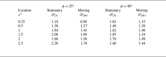
Table 3 summarises the non-dimensional dispersion
 $\mathscr{D}$
for both ground conditions for two rear slant angles. It can be seen that, among both the rear slant angles, the values of
 $\mathscr{D}$
, for locations closer to the Ahmed body (
 $x^*\leqslant 1)$
, are higher for
 $\phi =40^\circ$
irrespective of the ground conditions. This is due to the massive flow separation, backflow at the rear slant surface and the longer recirculation region behind the
 $\phi =40^\circ$
model. However, as the downstream distance increases, the non-dimensional dispersion is found to be higher for
 $\phi =25^\circ$
. This is due to the fact that, in the region beyond the recirculation region, there exists a system of trailing vortices behind the
 $\phi =25^\circ$
model, which increases the dispersion compared with
 $\phi =40^\circ$
model where no trailing vortices exist that can further enhance the dispersion.
To estimate the errors in the non-dimensional dispersion
 $\mathscr{D}$
we first estimate the errors in
 $\langle C^* \rangle$
. The errors in
 $\langle C^* \rangle$
due to image noise are negligible due to the well-resolved bit depth of the images. The main error in
 $\langle C^* \rangle$
is due to the unresolved attenuation from the concentration fluctuations (Cholemari & Mathur Reference Cholemari and Mathur2025). Based on Cholemari et al. (Reference Cholemari, Vishnubhatla and Krishnan2024) (see figure 4 therein), we estimate this error to be at most approximately 1.5 % relative to the mean concentration
 $\langle C^* \rangle$
. The sensitivity analysis for
 $\mathscr{D}$
indicates that, while changing the value of
 $\varPsi$
by a factor of four, i.e. from 0.05 to 0.2, results in a typically change of approximately
 $23\,\%$
in the value of
 $\mathscr{D}$
, which is not a very large change. We estimate the errors in
 $\mathscr{D}$
as
 \begin{align} \delta \mathscr{D} =\frac {{\rm d}\mathscr{D}}{{\rm d}\varPsi }\times \delta \langle C^*\rangle, \end{align}
where
 ${\rm d}\mathscr{D}/{\rm d} \varPsi$
is evaluated at the considered value of
 $\varPsi =0.1$
, and the error in concentration
 $\delta \langle C^* \rangle$
is estimated as above, as 1.5 %, leading to error bars given in figure 20. Please note the error bars are smaller than the symbols. The mean magnitude of the error bars is
 $\pm 0.033$
.
Variation of non-dimensional dispersion
 $(\mathscr{D})$
with respect to downstream distance in the wake of Ahmed body with slant angles
 $\phi = 25^\circ$
and
 $40^\circ$
.

Figures 20(a) and 20(b) show the variation of non-dimensional dispersion (
 $\mathscr{D}$
) with the streamwise distance (
 $x^*$
) under stationary and moving ground conditions for rear slant angles
 $\phi =25^\circ$
and
 $\phi =40^\circ$
, respectively. Figures indicate that the non-dimensional dispersion
 $\mathscr{D}$
at a given location is higher for stationary ground compared with moving ground conditions, and this is consistent for both the rear slant angles. The vortex G in stationary ground condition corresponds to an increase in the vertical mixing (or transport) of smoke. In contrast, the absence of vortex G in the moving ground condition leads to reduced vertical spread of the smoke (please refer to figure 21). Further, as seen from the movement of critical flow points under different ground conditions (figure 13), the movement of the spanwise turbulent structures toward the ground also concentrates the smoke near the ground, as seen in the concentration fields (figures 17 and 18). Figure 21 schematically illustrates the impact of the ground conditions on the spanwise vortical structures and hence the dispersion of smoke in the near wake. We can see that the dominating turbulent structures in the recirculation region are spanwise in nature and hence are likely to affect the vertical dispersion of the smoke. To clearly see the directional effects of the ground condition on the dispersion, in the next section, we calculate the parameters that quantify the dispersion in the vertical and lateral directions.
Schematic representation of the flow structures for stationary and moving ground conditions in the near wake of the Ahmed body with rear slant angles
 $\phi =25^\circ$
and
 $\phi =40^\circ$
.

Figure 20 also indicates that, for
 $\phi =25^\circ$
, the non-dimensional dispersion increases with the streamwise distance
 $x^*$
, irrespective of the ground condition (this was also observed by earlier studies (Keita Reference Keita2018; Keita et al. Reference Keita, Mehel, Fokoua, Murzyn, Taniere, Arcen and Diourte2023) (refer to figure 20
a), while for the
 $\phi =40^\circ$
model, the non-dimensional dispersion
 $\mathscr{D}$
does not increase significantly with the streamwise distance (
 $x^*$
) in both ground conditions (refer to figure 20
b). This is because of the absence of large-scale turbulent structures (pair of trailing vortices) in the wake of the
 $\phi =40^\circ$
model, which limits the smoke spread beyond the recirculation region (typically
 $x^*\approx 1$
Richards et al. Reference Richards, Wright, Baker and Baxendale2002; Rodriguez et al. Reference Rodriguez, Murzyn, Mehel and Larrarte2017; Rodriguez et al. Reference Rodriguez, Murzyn, Mehel and Larrarte2020), and hence the non-dimensional dispersion does not increase significantly. Whereas, for the
 $\phi =25^\circ$
model, the large-scale trailing vortices dominate after the recirculation region (
 $x^*\approx 1$
), which increases the spread of smoke in lateral as well as vertical directions, which ultimately increases the overall non-dimensional dispersion.
The results above also suggest caution while interpreting concentration values in the wake when the ground conditions are not appropriately modelled. Since the source of pollution is at the start of the wake region, it is expected that a greater spreading of the wake in the cross-stream directions, with the same mean wind velocity, implies a lower concentration of the pollutant within the wake. Hence, an experiment with an incorrect boundary condition (a stationary floor) which results in a larger extent of cross-stream dispersion implies incorrectly lower levels of concentrations overall in the wake, leading to a false sense of security.
3.3.2. Dispersion length scales (
$\mathscr{L}_y$
and
$\mathscr{L}_z$
)


The non-dimensional dispersion (
 $\mathscr{D}$
) effectively quantifies the overall dispersion in the wake; however, it does not provide insight into the individual lateral (
 $z$
) and vertical (
 $y$
) extents of smoke spread. To address this, we introduce parameters representing the dispersion in the respective directions. Given the complex and varying shapes of the dispersion patterns for different rear slant angles and wind tunnel ground conditions, a direct measurement of lateral and vertical dispersion is challenging. The non-dimensional dispersion length scales (
 $\mathscr{L}_y$
and
 $\mathscr{L}_z$
) are introduced to quantify the dispersion in the vertical and lateral directions, respectively. Dispersion length scales are obtained from the area under the dispersion envelope (
 $A_c$
) (shown by the blue line in figure 19
d), the centroid of the dispersion envelope (shown by ‘
 $*$
’ in figure 19
d) and the second moment of area of the dispersion envelope about its centroid (i.e.
 $I_{yy}$
and
 $I_{zz}$
). With these, an equivalent dispersion rectangle is defined as having the same area, the second moment of area and the centroid as those of the dispersion envelope. The equivalent dispersion rectangle is shown by the red line in figure 19(d). This rectangle represents the lateral and vertical dispersion of the smoke in the wake. The height and breadth of the equivalent dispersion rectangle provide the dispersion length scale in the vertical and lateral directions. Non-dimensional dispersion length scales in vertical and lateral directions are defined as follows:
 \begin{equation} \text{$\mathscr{L}_y$}=\frac {\text{$h_r$}}{\text{$h$}}; \text{$\mathscr{L}_z$}=\frac {\text{$b_r$}}{\text{$h$}}, \end{equation}
where
 $h_r$
and
 $b_r$
represent the height and width of the equivalent dispersion rectangle, respectively. The lengths
 $h_r$
and
 $b_r$
are non-dimensionalised by the Ahmed body height
 $h$
. To estimate the errors in the non-dimensional dispersion length scales,
 $\mathscr{L}_y$
and
 $\mathscr{L}_z$
, we proceed similarly as we did for the non-dimensional dispersion
 $\mathscr{D}$
above. The sensitivity analysis for
 $\mathscr{L}_y$
and
 $\mathscr{L}_z$
, indicates that, changing the values of
 $\varPsi$
from 0.05 to 0.2 results in a typical changes of approximately
 $14\,\%$
and
 $8.2\,\%$
in the values of
 $\mathscr{L}_y$
and
 $\mathscr{L}_z$
, respectively, which are not very large.
We estimate the errors in
 $\mathscr{L}_y$
and
 $\mathscr{L}_z$
, as
 \begin{align} \delta \mathscr{L}_y =\frac {{\rm d}\mathscr{L}_y}{{\rm d}\varPsi }\times \delta \langle C^*\rangle ;\;\; \delta \mathscr{L}_z =\frac {{\rm d}\mathscr{L}_z}{{\rm d}\varPsi }\times \delta \langle C^*\rangle, \end{align}
where
 ${\rm d}\mathscr{L}_y/{\rm d} \varPsi$
and
 ${\rm d}\mathscr{L}_z/{\rm d}\varPsi$
are evaluated from the sensitivity analysis at
 $\varPsi =0.1$
, and the error in concentration
 $\delta \langle C^*\rangle$
is estimated as above as 1.5 % (Cholemari et al. Reference Cholemari, Vishnubhatla and Krishnan2024), leading to error bars for
 $\mathscr{L}_y$
and
 $\mathscr{L}_z$
given in figures 22 and 23, respectively, with the mean magnitudes of the error bars being
 $\pm 0.013$
and
 $\pm 0.014$
, respectively. Please note the error bars are smaller than the symbols.
Tables 4 and 5 present the dispersion length scales for various downstream locations, ground conditions and rear slant angles. Figures 22(a) and 22(b) show the vertical dispersion length scale
 $(\mathscr{L}_y)$
variation with the streamwise distance in the near wake for rear slant angles
 $\phi =25^\circ$
and
 $\phi =40^\circ$
, respectively, for both ground conditions. Notably, the figures indicate a greater
 $\mathscr{L}_y$
consistently and, hence, vertical dispersion of smoke under stationary ground conditions across all downstream locations for both of the rear slant angles. This is in agreement with the observations from concentration contours, where it was observed that the smoke is more concentrated near the ground in the moving ground case. The increase in the vertical dispersion of the smoke can be attributed to the presence of vortex G in the stationary ground case, which is not present in the moving ground case, hence the reduced dispersion. This is also depicted schematically in figure 21.
Non-dimensional vertical dispersion length scales
 $(\mathscr{L}_y)$
at various downstream locations (
 $x^*$
) in the Ahmed body wake.

Non-dimensional lateral dispersion length scales
 $(\mathscr{L}_z)$
at various downstream locations (
 $x^*$
) in the Ahmed body wake.

Variation of non-dimensional dispersion length scales in vertical
 $(\mathscr{L}_y)$
directions with respect to downstream distance (
 $x^*$
) in the wake of Ahmed body with rear slant angles
 $\phi = 25^\circ$
and
 $40^\circ$
.

Variation of non-dimensional dispersion length scales in lateral
 $(\mathscr{L}_z)$
directions with respect to downstream distance (
 $x^*$
) in the wake of Ahmed body with rear slant angles
 $\phi = 25^\circ$
and
 $40^\circ$
.

Figures 23(a) and 23(b) show the variation of lateral dispersion length scale
 $(\mathscr{L}_z)$
with the streamwise distance (
 $x^*$
) in the near wake for rear slant angles
 $\phi =25^\circ$
and
 $\phi =40^\circ$
, respectively, for both of the ground conditions. It is observed that the lateral dispersion of the smoke shows an increasing trend along the streamwise distances (
 $x^*$
) in both the ground conditions and both the rear slant angles. Importantly, unlike the vertical dispersion length scale
 $(\mathscr{L}_y)$
, the lateral dispersion length scales
 $(\mathscr{L}_z)$
show a very slight difference among stationary and moving ground conditions for both the rear slant angles. This strongly implies that the existence of a ground vortex (vortex G) significantly affects the vertical dispersion and not the lateral dispersion of the smoke. Several studies (Zhang et al. Reference Zhang, Zhou and To2015; Venning et al. Reference Venning, Lo Jacono, Burton, Thompson and Sheridan2017; Liu et al. Reference Liu, Zhang, Zhang and Zhou2021) shows that the recirculation vortices (vortices A and B) are organised in the spanwise direction in the wake structure along the Ahmed body width. Since the ground vortex (vortex G) is also oriented in the spanwise direction, it is expected to strongly affect the vertical dispersion while the lateral dispersion is not affected much. Additionally, the shear in the
 $y$
direction only is altered, and the shear in the spanwise direction does not change due to the ground condition. Hence, the lateral transport/dispersion is not expected to change, as observed in figure 23. The increase in the vertical spread due to the ground conditions leads to an increase in the overall smoke dispersion in the wake, which manifests as the increase in the non-dimensional dispersion
 $\mathscr{D}$
in the stationary ground condition (refer to figure 20).
It is important to note that the vertical dispersion length scale
 $(\mathscr{L}_y)$
shows an increasing trend for
 $\phi =25^\circ$
(figure 22
a). However, a decreasing trend of the same
 $(\mathscr{L}_y)$
is observed for
 $\phi =40^\circ$
(figure 22
b). This shows that the vertical dispersion of smoke increases for the subcritical rear slant angle
 $\phi \lt \phi _c$
(due to the presence of large-scale trailing vortices in the wake). However, it decreases for the supercritical rear slant angle
 $\phi \gt \phi _c$
(due to the absence of large-scale trailing vortices in the wake). This strongly agrees with the earlier observation by Mathur et al. (Reference Mathur, Cholemari and Veeravalli2024b
), where they found similar trends in the smoke spread (
 $S_y$
) with the streamwise distance (
 $x^*$
) behind the Ahmed body with rear slant angles,
 $\phi =25^\circ$
and
 $\phi =40^\circ$
, with stationary ground conditions in the wind tunnel. In the present study, similar trends of dispersion growth (with the streamwise distance
 $x^*$
) are observed for the moving ground conditions, suggesting that the overall growth rate of the dispersion parameters is either insignificantly or not at all affected by the ground conditions. This can also be verified from the similar trends of dispersion parameters with the streamwise distance (
 $x^*$
), for both ground conditions. In the case of
 $\phi =25^\circ$
, there exists a system of trailing vortices in the wake, which grows in size as streamwise distance (
 $x^*$
) increases. These vortices further mix the smoke particles to increase the dispersion length scales. Such a system of trailing vortices does not exist behind the
 $\phi =40^\circ$
case. The smoke particle transport behind the
 $\phi =40^\circ$
model is driven by the shear between the ground and the flow (when floor is stationary). As the streamwise distance increases, the turbulence in the wake reduces and, therefore, the smoke transport also reduces. Due to this, the dispersion length scales come down to the level of the moving case where there is no shear between flow and moving ground. Comparing the
 $\mathscr{L}_y$
and
 $\mathscr{L}_z$
values in tables 4 and 5 reveals that the lateral spread of smoke consistently exceeds the vertical spread, regardless of downstream location or ground conditions.
Increase in non-dimensional dispersion (
 $\Delta \mathscr{D}$
) and dispersion length scales (
 $\Delta \mathscr{L}_y, \Delta \mathscr{L}_z$
) at various downstream locations for
 $\phi =25^\circ$
, comparing stationary and moving ground conditions.

Increase in non-dimensional dispersion (
 $\Delta \mathscr{D}$
) and dispersion length scales (
 $\Delta \mathscr{L}_y, \Delta \mathscr{L}_z$
) at various downstream locations for
 $\phi =40^\circ$
, comparing stationary and moving ground conditions.

To quantify the change in the smoke dispersion due to the different wind tunnel ground conditions, we calculate the change in the dispersion parameters. The change in the dispersion parameters is calculated based on the following equations:
 \begin{equation} \Delta \mathscr{D}(x^*)=\bigg (\frac {\mathscr{D}(x^*)|_{St}- \mathscr{D}(x^*)|_{Mv}}{\mathscr{D}(x^*)|_{Mv}}\bigg ), \end{equation}
 \begin{equation} \Delta \mathscr{L}_y(x^*)=\bigg (\frac {\mathscr{L}_y(x^*)|_{St}- \mathscr{L}_y(x^*)|_{Mv}}{\mathscr{L}_y(x^*)|_{Mv}}\bigg ), \end{equation}
 \begin{equation} \Delta \mathscr{L}_z(x^*)=\bigg (\frac {\mathscr{L}_z(x^*)|_{St}- \mathscr{L}_z(x^*)|_{Mv}}{\mathscr{L}_z(x^*)|_{Mv}}\bigg ). \end{equation}
Tables 6 and 7 show the change in the dispersion parameters between stationary and moving ground conditions for both the rear slant angles of the Ahmed body. From the tables, it can be seen that there is a significant change in the dispersion parameter due to the wind tunnel ground conditions. For
 $\phi =25^\circ$
, maximum increase in the dispersion parameters is observed as:
 $\Delta \mathscr{D}=30\,\%$
,
 $\Delta \mathscr{L}_y=29\,\%$
and
 $\Delta \mathscr{L}_z=6\,\%$
. Mathur et al. (Reference Mathur, Bhanu, Cholemari and Veeravalli2025) also observed a
 $\approx 30\,\%$
increase in the vertical spread (
 $S_y$
) of the smoke in the stationary ground case compared with the moving ground case, in agreement with the present results. For
 $\phi =40^\circ$
, maximum increase in the dispersion parameters is observed as:
 $\Delta \mathscr{D}=38\,\%$
,
 $\Delta \mathscr{L}_y=49\,\%$
and
 $\Delta \mathscr{L}_z=12\,\%$
. This highlights the significant influence of the wind tunnel ground conditions on the dispersion in the Ahmed body wake. The results suggest that the wind tunnel ground condition is a critical aspect to address while performing dispersion measurements behind the Ahmed body in a wind tunnel.
4. Summary and conclusions
Wind tunnel ground conditions significantly alter the flow structures and influence the dispersion phenomenon in the wake of the Ahmed body; therefore, it is a critical aspect to address while performing physically correct dispersion studies behind a vehicle in the wind tunnel. This study presents a comprehensive experimental investigation into the impact of wind tunnel ground conditions (stationary vs. moving) on flow structures, smoke concentration and dispersion in the near wake of an Ahmed body. Experiments were conducted at
 $\textit{Re}_l = 1.21 \times 10^5$
across two critical wake flow regimes, using rear slant angles of
 $\phi = 25^{\circ }$
and
 $40^{\circ }$
, with stationary and moving ground conditions. The moving ground condition, established using a rolling road and boundary layer suction system, allowed us to implement Galilean transformation and accurately simulate a vehicle moving through still air. This study uses quantitative methodology to address key gaps in the current literature in the field of vehicle wake dispersion modelling and vehicle aerodynamics.
Specifically, we conducted the first detailed dispersion experiments comparing stationary and moving ground conditions, providing a direct assessment of the effect of ground conditions on the dispersion in the Ahmed body wake. We successfully performed field measurements of both velocity (using PIV) and concentration (using non-intrusive QSV) within the identical experimental set-up, which has not previously been done. This allowed us to directly correlate the velocity and concentration fields, establishing a link between the observed flow structures (like spanwise and trailing vortex systems) and the resulting dispersion behaviour. Finally, we quantify the dispersion through the definition and calculation of novel dispersion parameters: non-dimensional dispersion (
 $\mathscr{D}$
), and vertical and lateral dispersion length scales (
 $\mathscr{L}_y,\mathscr{L}_z$
). These calculated parameters, derived from the concentration fields measured across six downstream locations (
 $x^* = 0.25$
to
 $2.5$
), provide the essential quantitative parameters for evaluating the critical role of the ground conditions.
Major findings from the present study:
A. The critical role of ground vortex (vortex G):
-
(i) In the stationary ground condition, the formation of a third spanwise vortex (i.e. the ground vortex, referred to as vortex G) is observed, which is not observed in moving ground cases. In the present study, the identification of vortex G provides the physical explanation for the observed changes in the scalar dispersion in the vehicle wake, under different wind tunnel ground conditions.
-
(ii) The correlation between the velocity field with the concentration field shows the link between the presence of the ground vortex (vortex G) and the quantifiable increase in the dispersion parameters for the stationary ground cases. Vortex G causes an increase in the transport of smoke preferentially in the vertical direction (figure 21), due to its spanwsie orientation. As a consequence, the vertical dispersion length scales (
$\mathscr{L}_y$
) and non-dimensional dispersion (
$\mathscr{D}$
) are higher than those for the moving ground condition (figure 20, 22). -
(iii) The absence of the ground vortex (vortex G) in the moving ground condition reduces the vertical position of dominating spanwise turbulent structures in the recirculation region, as shown by the movement of the critical flow points (figure 13). The moving ground enhances the underbody flow, causing an extended recirculation region.


B. Quantifying the significant impact on dispersion parameters:
-
(i) The present study defines physically accurate dispersion parameters (
$\mathscr{D}$
,
$\mathscr{L}_y$
and
$\mathscr{L}_z$
) obtained from the concentration fields data, which confirm and significantly refine previously reported dispersion trends (Mathur et al. Reference Mathur, Bhanu, Cholemari and Veeravalli2025). The dispersion analysis shows a considerable overestimation of dispersion in the stationary ground conditions. -
(ii) The non-dimensional dispersion
$\mathscr{D}$
(figure 20) is consistently greater for stationary ground conditions across all downstream locations (
$x^*$
). The maximum increase in the non-dimensional dispersion (
$\Delta \mathscr{D}$
) is
$\approx$
30 % when
$\phi =25^\circ$
and
$\approx$
38 % when
$\phi =40^\circ$
, highlighting the significant impact of wind tunnel ground conditions on the dispersion in the near wake. -
(iii) The vertical dispersion length scale
$\mathscr{L}_y$
(figure 22) is consistently greater and shows a significant overestimation for stationary ground conditions across all downstream locations (
$x^*$
). The maximum increase in the vertical dispersion length scale (
$\Delta \mathscr{L}_y$
) is
$\approx$
29 % when
$\phi =25^\circ$
and
$\approx$
49 % when
$\phi =40^\circ$
, highlighting that the vertical dispersion is more influenced by the wind tunnel ground conditions. -
(iv) The lateral dispersion length scales
$\mathscr{L}_z$
remain nearly the same for both stationary and moving ground conditions (figure 23), indicating that lateral dispersion is hardly influenced by ground condition variations. This is a consequence of the fact that the shear in the
$y$
direction only is altered in the moving ground case.


C. Impact of the rear slant angle and its link to ground conditions:
-
(i) Increase in the rear slant angle causes a vertically upward movement of the
$F_1$
critical point, increasing the height of recirculation region, while
$F_2$
and SP critical points move horizontally, increasing the length of the recirculation region, indicated by significantly increased values of
$L^*_R$
. -
(ii) The vertical dispersion of the smoke is enhanced behind the
$\phi =40^\circ$
model, when compared with the
$\phi =25^\circ$
model, due to the separation on the rear slant. However, it is also observed that the wind tunnel ground condition affects the flow topology in a similar way for both the rear slant angles (the flow topology, despite being significantly different for both angles).


The above points demonstrate the importance of using physically correct boundary conditions during experimental investigation of moving vehicle in a wind tunnel.
Future outlook: overall, this study provides quantitative evidence demonstrating the critical role of accurate ground condition modelling in wind tunnel study of dispersion in vehicle wakes. The correlation established between the velocity and concentration field measurements conclusively proves that the ground vortex (vortex G) significantly alters the near-wake flow and leads to a substantial, quantifiable overestimation of vertical smoke dispersion in stationary floor wind tunnels. These findings underscore the fundamental importance of employing moving ground and boundary layer suction systems when conducting wind tunnel experiments on vehicle wakes for dispersion and aerodynamic research.
This study correctly implements the Galilean transformation in the wind tunnel to simulate a vehicle moving in still ambient air. Other combinations of boundary layer suction and moving ground (with different velocities) can simulate other conditions, such as a vehicle moving into head/tail wind conditions. Additionally, the standard Ahmed body does not provide the location of the smoke exhaust. It is indeed worthwhile to study the position of the exhaust and the influence of the ground clearance on the flow dynamics. Another aspect is the existence of ground vortex (vortex G) that can be significantly dictated by various geometrical parameters (e.g. ground clearance, aspect ratio and rear slant angle of the Ahmed body) and flow parameters (free-stream velocity, boundary layer thickness). Future research should focus on utilising the quantitative methodology described in this study to investigate the above mentioned aspects of the problem.
Acknowledgements
The authors gratefully acknowledge Mr S.H. Vishnubhatla for his help in the PIV and QSV experiments.
Declaration of interests
The authors report no conflicts of interest.