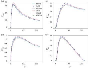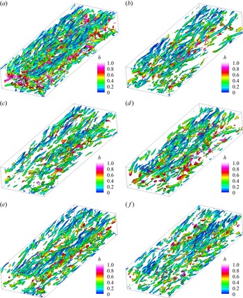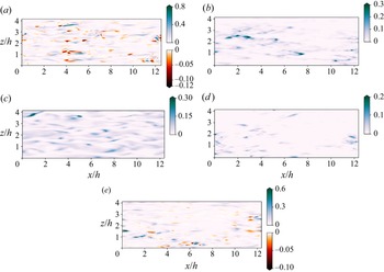

1. Introduction
Turbulent flows have the intrinsic multi-scale characteristics across several orders of magnitude, therefore direct numerical simulation (DNS) of turbulence at high Reynolds numbers is extremely time consuming and not tractable to solve all flow scales ranging from the dissipation range to the energy-containing range. Accordingly, the large-eddy simulation (LES) is an effective approach in which only the large-scale motions are resolved while the effect of the residual subgrid-scale (SGS) structures on the resolved large-scale motions are modelled by an SGS model (Lesieur & Metais Reference Lesieur and Metais1996; Meneveau & Katz Reference Meneveau and Katz2000; Sagaut Reference Sagaut2006; Garnier, Adams & Sagaut Reference Garnier, Adams and Sagaut2009; Durbin Reference Durbin2018; Moser, Haering & Yalla Reference Moser, Haering and Yalla2021). Extensive SGS models have been proposed to reconstruct the unclosed SGS terms in previous works, and the eddy-viscosity SGS models (Smagorinsky Reference Smagorinsky1963; Deardorff Reference Deardorff1970; Nicoud & Ducros Reference Nicoud and Ducros1999; Vreman Reference Vreman2004) are often utilised due to the dissipative nature of the SGS stress tensor. In eddy-viscosity SGS models, the Smagorinsky model (Smagorinsky Reference Smagorinsky1963; Deardorff Reference Deardorff1970) is one of the most widely used SGS models whose model coefficient is statically calibrated by the experimental and numerical data. Germano et al. (Reference Germano, Piomelli, Moin and Cabot1991) pioneered the famous dynamic procedure based on the Germano identity, which makes the coefficients of the dynamic Smagorinsky model (DSM) dynamically modified as the flow evolves. Subsequently, other improved and generalised dynamical versions of the Smagorinsky model were introduced by Lilly (Reference Lilly1992), Piomelli (Reference Piomelli1993), Ghosal et al. (Reference Ghosal, Lund, Moin and Akselvoll1995) and Meneveau, Lund & Cabot (Reference Meneveau, Lund and Cabot1996). Furthermore, Nicoud & Ducros (Reference Nicoud and Ducros1999) proposed a wall-adapting local eddy-viscosity model (WALE), which has a good performance in wall-bounded turbulence. Moreover, Vreman (Reference Vreman2004) introduced another eddy-viscosity model with quite satisfactory results in turbulent shear flows.
The eddy-viscosity models assume that the SGS stress is linearly aligned with the filtered strain-rate tensor based on the Boussinesq hypothesis. Therefore, these eddy-viscosity models have a serious drawback that they correlate poorly with the true SGS stress (Anderson & Meneveau Reference Anderson and Meneveau1999; Da Silva & Métais Reference Da Silva and Métais2002) and cannot predict the energy backscatter to the resolved scales (Zang, Street & Koseff Reference Zang, Street and Koseff1993). Furthermore, the linear alignment assumption in the eddy-viscosity models is unphysical and cannot estimate the complicated nonlinear relation between the filtered strain-rate tensor and the SGS stress (Anderson & Meneveau Reference Anderson and Meneveau1999; Da Silva & Métais Reference Da Silva and Métais2002; Xie et al. Reference Xie, Li, Ma and Wang2019a,Reference Xie, Wang, Li and Mac; Xie, Wang & Weinan Reference Xie, Wang and Weinan2020a; Xie, Yuan & Wang Reference Xie, Yuan and Wang2020b). In order to alleviate these problems, Pope (Reference Pope1975) derived a general nonlinear algebraic expression between the Reynolds stress and the averaged strain-rate and rotation-rate tensors with ten integrity bases based on the theory of invariants. Furthermore, Lund & Novikov (Reference Lund and Novikov1992) reduced the ten integrity basis tensors to five, which significantly simplified the computational complexity of the nonlinear algebraic SGS model. Similarly, Wang et al. (Reference Wang, Yin, Yee and Bergstrom2007) proposed a dynamic nonlinear tensorial diffusivity model to model the SGS scalar flux in the incompressible turbulence. Then, how to determine the model coefficients in the nonlinear algebraic models is a significant issue. In the early stages, the model coefficients were mostly determined by the experimental and numerical data. Recently, the dynamical versions of these nonlinear algebraic SGS models (Wang et al. Reference Wang, Yin, Yee and Bergstrom2007; Yuan et al. Reference Yuan, Wang, Xie and Wang2022) were proposed and exhibited a reasonable agreement with the filtered DNS (fDNS) data. Furthermore, Wang et al. (Reference Wang, Yuan, Xie and Wang2021b) proposed a dynamic spatial gradient model, which has good performance in both a priori and a posteriori tests in LES of incompressible isotropic turbulence. However, the dynamic approach requires some ad hoc procedures, including the averaging of model coefficients in statistically homogeneous directions and the clipping of the negative model coefficients to avoid numerical instability.
Recently, the artificial neural network (ANN) has become a popular approach to develop SGS models (Gamahara & Hattori Reference Gamahara and Hattori2017; Vollant, Balarac & Corre Reference Vollant, Balarac and Corre2017; Beck, Flad & Munz Reference Beck, Flad and Munz2019; Maulik et al. Reference Maulik, San, Rasheed and Vedula2019; Xie et al. Reference Xie, Li, Ma and Wang2019a,Reference Xie, Wang, Li and Mac; Yang et al. Reference Yang, Zafar, Wang and Xiao2019; Zhou et al. Reference Zhou, He, Wang and Jin2019; Xie et al. Reference Xie, Yuan and Wang2020b; Yuan, Xie & Wang Reference Yuan, Xie and Wang2020; Frezat et al. Reference Frezat, Balarac, Le Sommer, Fablet and Lguensat2021; Park & Choi Reference Park and Choi2021; Yu et al. Reference Yu, Yuan, Qi, Wang, Li and Chen2022). The ANN method can construct a complex nonlinear mapping between some resolved flow variables and the unresolved SGS terms. Therefore, the SGS models based on the ANN method are expected to give more accurate prediction than the traditional SGS models, and have a good performance in a posteriori tests of compressible and incompressible isotropic turbulence (Xie et al. Reference Xie, Li, Ma and Wang2019a,Reference Xie, Wang, Li and Mac, Reference Xie, Yuan and Wang2020b) and incompressible channel flow (Park & Choi Reference Park and Choi2021). It is worth noting that the ANN-based SGS models can get rid of the averaging procedure of the model coefficients in statistically homogeneous directions. Furthermore, the ANN-based SGS models in compressible and incompressible isotropic turbulence (Xie et al. Reference Xie, Li, Ma and Wang2019a,Reference Xie, Wang, Li and Mac, Reference Xie, Yuan and Wang2020b) and the single-point ANN-based SGS model in the incompressible channel flow (Park & Choi Reference Park and Choi2021) are free from backscatter clipping, while the multi-point ANN-based SGS model in incompressible channel flow (Park & Choi Reference Park and Choi2021) requires the backscatter clipping procedure.
The ANN method was also used to determine the model coefficients in the nonlinear algebraic models. Ling, Kurzawski & Templeton (Reference Ling, Kurzawski and Templeton2016) firstly used the deep neural networks to predict the model coefficients of the ten isotropic basis tensors given by Pope (Reference Pope1975) to obtain an improved Reynolds-averaged Navier–Stokes model. Similarly, Xie et al. (Reference Xie, Yuan and Wang2020b) proposed ANN-based nonlinear algebraic SGS models in LES of incompressible isotropic turbulence. They constructed a neural network mapping between four dimensionless invariants and five model coefficients given by Lund & Novikov (Reference Lund and Novikov1992), and this new model exhibited a better performance in a priori and a posteriori tests than traditional SGS models. Moreover, Vollant et al. (Reference Vollant, Balarac and Corre2017) proposed a new ANN-based SGS model for the LES of a passive scalar in the incompressible turbulence. Wang et al. (Reference Wang, Yuan, Xie and Wang2021a) proposed an artificial neural network-based spatial gradient models in LES of incompressible isotropic turbulence, which used the ANN method to estimate the coefficients of the spatial gradient models.
The above studies mainly concentrated on ANN-based LES of incompressible turbulence; however, there are much fewer studies aiming to apply the ANN method to develop the well-performing SGS models for the compressible wall-bounded flows. It is worth noting that, due to the remarkable influence of compressibility, the underlying mechanisms of the compressible wall-bounded turbulence are much more complex than those in incompressible turbulence (Maeder, Adams & Kleiser Reference Maeder, Adams and Kleiser2001; Pirozzoli, Grasso & Gatski Reference Pirozzoli, Grasso and Gatski2004; Pirozzoli, Bernardini & Grasso Reference Pirozzoli, Bernardini and Grasso2008; Duan, Beekman & Martin Reference Duan, Beekman and Martin2010; Pirozzoli, Bernardini & Grasso Reference Pirozzoli, Bernardini and Grasso2010; Lagha et al. Reference Lagha, Kim, Eldredge and Zhong2011; Pirozzoli & Bernardini Reference Pirozzoli and Bernardini2011; Xu et al. Reference Xu, Wang, Wan, Yu, Li and Chen2021a,Reference Xu, Wang, Wan, Yu, Li and Chenb, Reference Xu, Wang, Yu, Li and Chen2022b,Reference Xu, Wang, Yu, Li and Chenc; Xu, Wang & Chen Reference Xu, Wang and Chen2022a), and the study of improved SGS models in compressible wall-bounded flows is of extraordinary importance in the aerospace industry. Recently, Yu et al. (Reference Yu, Yuan, Qi, Wang, Li and Chen2022) proposed a new eddy-viscosity SGS model constrained by the ANN-based modelling of the kinetic energy flux for LES of compressible wall-bounded turbulence. The new kinetic-energy-flux-constrained model (KCM) showed a better performance in a priori and a posteriori tests than the traditional SGS models. However, Yu et al. (Reference Yu, Yuan, Qi, Wang, Li and Chen2022) only constructed a good SGS model for the unclosed SGS stress tensor, while advanced SGS models for the unclosed SGS heat flux are much less investigated, which are significant in the LES of compressible wall-bounded turbulence. Furthermore, the KCM developed by Yu et al. (Reference Yu, Yuan, Qi, Wang, Li and Chen2022) is essentially an eddy-viscosity model. It is assumed by KCM that the SGS stress and SGS heat flux are linearly correlated with the filtered strain-rate tensor and the gradient of the filtered temperature respectively. These linear alignment assumptions are unphysical and it can be speculated that the predicted SGS stress and SGS heat flux estimated by KCM would not have high correlations with the true SGS stress and SGS heat flux. The KCM also cannot estimate the complicated nonlinear relation between the filtered strain-rate tensor and the SGS stress as well as the gradient of the filtered temperature and the SGS heat flux.
It is worth noting that a critical issue for the ANN-based SGS model is the generalisation ability to untrained flow conditions. Park & Choi (Reference Park and Choi2021) showed that an ANN-based model trained at a single grid resolution did not predict the flow statistics accurately at another grid resolution, and this conclusion was also found in Zhou et al. (Reference Zhou, He, Wang and Jin2019). However, many studies have shown that an ANN-based SGS model trained at low Reynolds number also has a good performance at high Reynolds number (Maulik et al. Reference Maulik, San, Rasheed and Vedula2019; Park & Choi Reference Park and Choi2021).
Another significant issue for the ANN-based model is the much larger computational cost, as compared with those of the conventional dynamic eddy-viscosity models. It is shown that the computational cost of the ANN-based models given in Park & Choi (Reference Park and Choi2021), Wang et al. (Reference Wang, Luo, Li, Tan and Fan2018b), Yuan et al. (Reference Yuan, Xie and Wang2020), Xie et al. (Reference Xie, Wang, Li and Ma2019c) and Xie et al. (Reference Xie, Wang and Weinan2020a) were approximately 1.3, 1.8, 2.4, 15 and 256 times of that of DSM, respectively. Furthermore, the ANN-based model in Yu et al. (Reference Yu, Yuan, Qi, Wang, Li and Chen2022) was also time consuming due to the large number of the neurons of the hidden layer and the complex hyperbolic tangent (tanh) activation function.
Accordingly, the main objective of this study is to propose a well-performing ANN-based nonlinear algebraic model for the LES of compressible wall-bounded turbulence for the first time. The nonlinear algebraic model of the SGS stress tensor proposed by Lund & Novikov (Reference Lund and Novikov1992) and that of the SGS passive scalar flux given by Wang et al. (Reference Wang, Yin, Yee and Bergstrom2007) in the incompressible turbulence are modified to utilise in the compressible turbulent channel flow. The ANN method is used to estimate the dimensionless model coefficients in order to get rid of some ad hoc procedures such as the averaging of model coefficients in statistically homogeneous directions and the clipping of the negative model coefficients to avoid numerical instability. Furthermore, the new model is trained with compressible turbulent channel flow data at a single Reynolds number, Mach number and grid resolution, and can have better performance in predicting the flow statistics in compressible turbulent channel flows with untrained Reynolds numbers, Mach numbers and grid resolutions. Moreover, the new model can also accurately predict the flow statistics in the supersonic turbulent boundary layer. Finally, the proposed models are more computationally efficient than the DSM, and make more accurate predictions than the conventional SGS models.
The rest of the paper is organised as follows. The governing equations of the LES and the a priori test of the traditional SGS models are described in § 2. The structure and the a priori test of the ANN-based nonlinear algebraic model are shown in § 3. The a posteriori test of the modified ANN-based nonlinear algebraic model is presented in § 4. Finally, summary and conclusions are given in § 5.
2. The governing equations of the LES and the a priori test of the traditional SGS models
2.1. The governing equations of the LES
By applying the filtering method to Navier–Stokes equations, the following compressible dimensionless LES governing equations are derived (Garnier et al. Reference Garnier, Adams and Sagaut2009):
 \begin{align} \frac{\partial \bar{\rho }}{\partial t}&+\frac{\partial ( \bar{\rho } \tilde{u}_{j} )}{\partial x_{j}}=0, \end{align}
 \begin{align}\frac{\partial \left ( \bar{\rho} \tilde{u}_{i} \right )}{\partial t}+\frac{\partial [ \bar{\rho} \tilde{u}_{i}\tilde{u}_{j}+\bar{p}\delta _{ij} ]}{\partial x_{j}}&=\frac{1}{Re}\frac{\partial \tilde{\sigma} _{ij}}{\partial x_{j}}-\frac{\partial \bar{\rho}\tau _{ij}}{\partial x_{j}}+\frac{1}{Re}\frac{\partial }{\partial x_{j}}( \overline{\sigma _{ij}}- \tilde{\sigma} _{ij}), \end{align}
 \begin{align}\frac{\partial \bar{\rho }\tilde{E}}{\partial t} +\frac{\partial [ ( \bar{\rho }\tilde{E}+\bar{p} )\tilde{u}_{j} ]}{\partial x_{j}}&=\frac{1}{Re}\frac{\partial ( \tilde{\sigma} _{ij}\tilde{u}_{i} )}{\partial x_{j}}-\frac{1}{\alpha }\frac{\partial \tilde{q}_{j}}{\partial x_{j}}-\frac{\partial ( C_{p}\bar{\rho}Q_{j} )}{\partial x_{j}}-\frac{\partial \mathcal{J}_{j}}{\partial x_{j}}\nonumber\\ & +\frac{\partial }{\partial x_{j}}[ ( \overline{\sigma _{ij}u_{i}}-\tilde{\sigma} _{ij}\tilde{u}_{i} )+( \overline{q_{j}}-\tilde{q}_{j} ) ], \end{align}
 \begin{align}&\quad \quad \bar{p}=\bar{\rho} \tilde{T}/( \gamma M^{2} ). \end{align}
Here,  $\bar {\rho }$,
 $\tilde {u}_{i}$,
 $\tilde {T}$,
 $\bar {p}$ represent the resolved density, velocity, temperature and pressure, respectively, and
 $\bar {\rho }\tilde {E}$ is the Favre-averaged total energy defined later in (2.13). The filtered field for a variable
 $f$ can be defined as (Martin, Piomelli & Candler Reference Martin, Piomelli and Candler2000; Xu et al. Reference Xu, Wang, Wan, Yu, Li and Chen2021b)
 \begin{equation} \bar{f}\left ( \boldsymbol{x} \right )=\int \,{\rm d}^{3}\boldsymbol{r}G_{l}\left ( \boldsymbol{r} \right )f\left ( \boldsymbol{x}+\boldsymbol{r} \right ), \end{equation}
where  $G_{l} ( \boldsymbol {r} )\equiv l^{-3}G ( \boldsymbol {r}/l )$ is the filter function, and
 $G ( \boldsymbol {r} )$ is a normalised window function. Here,
 $l$ is the filter width associated with the wavelength of the smallest scale retained by the filtering operation. The symbol
 $\tilde {f}=\overline{\rho f}/\bar {\rho }$ represents the Favre filtered field.
The above compressible LES equations are non-dimensionalised by the following set of reference scales, including the reference length  $L_{\infty }$, free-stream density
 $\rho _{\infty }$, velocity
 $U_{\infty }$, temperature
 $T_{\infty }$, pressure
 $p_{\infty }= \rho _{\infty }U_{\infty }^{2}$, energy per unit volume
 $\rho _{\infty }U_{\infty }^{2}$, viscosity
 $\mu _{\infty }$ and thermal conductivity
 $\kappa _{\infty }$. The ratio of specific heat at constant pressure
 $C_{p}$ to that at constant volume
 $C_{v}$ is defined as
 $\gamma = C_{p}/C_{v}$ and assumed to be equal to 1.4. Moreover,
 $Re= \rho _{\infty }U_{\infty }L_{\infty }/\mu _{\infty }$ is the Reynolds number,
 $M= U_{\infty }/c_{\infty }$ is the Mach number and
 $\alpha = Pr\,Re ( \gamma -1 )M^{2}$, where the Prandtl number
 $Pr= \mu _{\infty } C_{p}/\kappa _{\infty }$ is equal to 0.7.
The resolved viscous stress tensor  $\tilde {\sigma } _{ij}$ and the resolved heat flux
 $\tilde {q}_{j}$ are defined as
 \begin{equation} \tilde{\sigma} _{ij}=2\tilde{\mu } ( \tilde{T} )( \tilde{S}_{ij}-\tfrac{1}{3}\delta _{ij}\tilde{S}_{kk} ) \end{equation}
and
 \begin{equation} \tilde{q}_{j}={-}\kappa ( \tilde{T} )\frac{\partial \tilde{T}}{\partial x_{j}}, \end{equation}
where  $\tilde {\mu }= ( \tilde {T}/\tilde {T}_{\infty } )^{3/2} [ ( \tilde {T}_{\infty }+T_{s} )/ ( \tilde {T}+T_{s} ) ]$ is the molecular viscosity calculated by Sutherland's law with
 $T_{s}=110.4\,{\rm K}$ and
 $\tilde {T}_{\infty }=288.15\,{\rm K}$, and the thermal conductivity
 $\tilde {\kappa }$ has the same expression as
 $\tilde {\mu }$. Furthermore,
 $\tilde {S}_{ij}=( \partial \tilde {u}_{i}/\partial x_{j}+\partial \tilde {u}_{j}/\partial x_{i} )/2$ is the resolved strain-rate tensor.
As was done in many previous studies, including Ragab, Sheen & Sreedhar (Reference Ragab, Sheen and Sreedhar1992), Piomelli (Reference Piomelli1999), Dubois, Domaradzki & Honein (Reference Dubois, Domaradzki and Honein2002), Kawai & Larsson (Reference Kawai and Larsson2013) and Yu et al. (Reference Yu, Yuan, Qi, Wang, Li and Chen2022), the unclosed terms  $({1}/{Re})({\partial }/{\partial x_{j}}) (\overline {\sigma _{ij}}- \tilde {\sigma } _{ij} )$ in (2.2) and
 $({\partial }/{\partial x_{j}}) [ ( \overline {\sigma _{ij}u_{i}}-\tilde {\sigma } _{ij}\tilde {u}_{i} )+ ( \overline {q_{j}}-\tilde {q}_{j} ) ]$ in (2.3) can be neglected, which is justified by the inviscid criterion introduced in Aluie (Reference Aluie2013) and Zhao & Aluie (Reference Zhao and Aluie2018). Therefore, (2.2) and (2.3) can be simplified to
 \begin{gather} \frac{\partial \left ( \bar{\rho} \tilde{u}_{i} \right )}{\partial t}+\frac{\partial [ \bar{\rho} \tilde{u}_{i}\tilde{u}_{j}+\bar{p}\delta _{ij} ]}{\partial x_{j}}=\frac{1}{Re}\frac{\partial \tilde{\sigma} _{ij}}{\partial x_{j}}-\frac{\partial \bar{\rho}\tau _{ij}}{\partial x_{j}}, \end{gather}
 \begin{gather} \frac{\partial \bar{\rho }\tilde{E}}{\partial t}+\frac{\partial [ ( \bar{\rho }\tilde{E}+\bar{p} )\tilde{u}_{j} ]}{\partial x_{j}}=\frac{1}{Re}\frac{\partial ( \tilde{\sigma} _{ij}\tilde{u}_{i} )}{\partial x_{j}}-\frac{1}{\alpha }\frac{\partial \tilde{q}_{j}}{\partial x_{j}}-\frac{\partial ( C_{p}\bar{\rho}Q_{j} )}{\partial x_{j}}-\frac{\partial \mathcal{J}_{j}}{\partial x_{j}}. \end{gather}
It is found that there are three unclosed terms in the above compressible LES equations, including the SGS stress tensor
 \begin{equation} \tau _{ij}=\widetilde{u_{i}u_{j}}-\tilde{u}_{i}\tilde{u}_{j}, \end{equation}
the SGS heat flux
 \begin{equation} Q_{j}=\widetilde{u_{j}T}-\tilde{u}_{j}\tilde{T}, \end{equation}
and the SGS turbulent diffusion
 \begin{equation} \mathcal{J}_{j}=\frac{1}{2}\bar{\rho }\left ( \widetilde{u_{j}u_{i}u_{i}}-\tilde{u}_{j}\widetilde{u_{i}u_{i}} \right ). \end{equation}
Moreover,  $\bar {\rho }\tilde {E}$ is the Favre-averaged total energy, and can be defined as
 \begin{equation} \bar{\rho }\tilde{E}=\frac{\bar{p}}{\gamma -1}+\frac{1}{2}\bar{\rho }\tilde{u}_{i}\tilde{u}_{i}+\frac{1}{2}\bar{\rho }\tau _{ii}. \end{equation}
Therefore, the resolved temperature  $\tilde {T}$ can be calculated by
 \begin{equation} \tilde{T}=\left ( \gamma -1 \right )\gamma M^{2}\left [ \tilde{E}-\frac{1}{2}\tilde{u}_{i}\tilde{u}_{i}-\frac{\tau _{ii}}{2} \right ]. \end{equation}
Furthermore, it is suggested that the SGS turbulent diffusion can be approximated by  $\mathcal {J}_{j}\approx \bar {\rho }\tau _{ij}\tilde {u}_{i}$ (Martin et al. Reference Martin, Piomelli and Candler2000; Jiang et al. Reference Jiang, Xiao, Shi and Chen2013; Yu et al. Reference Yu, Yuan, Qi, Wang, Li and Chen2022). Therefore, only the SGS stress tensor
 $\tau _{ij}$ and the SGS heat flux
 $Q_{j}$ need to be modelled based on the resolved variables.
It is noted that the subscripts  $i$ and
 $j$ of
 $\tau _{ij}$ and
 $Q_{j}$ satisfy
 $i,\,j=1, \,2, \,3$, where the numbers 1, 2, 3 represent the streamwise (
 $x$), wall-normal (
 $y$) and spanwise (
 $z$) directions, respectively.
2.2. The a priori test of the traditional SGS models
It is worth noting that the eddy-viscosity models are the most famous SGS models for the SGS stress tensor  $\tau _{ij}$ and the SGS heat flux
 $Q_{j}$. The DSM (Moin et al. Reference Moin, Squires, Cabot and Lee1991; Lilly Reference Lilly1992), the Vreman model (Vreman Reference Vreman2004; Sayadi & Moin Reference Sayadi and Moin2012) and the WALE model (Nicoud & Ducros Reference Nicoud and Ducros1999; Garnier et al. Reference Garnier, Adams and Sagaut2009) are the widely used SGS models, which are used to compared with the new proposed models in the present study.
The eddy-viscosity models of the SGS stress tensor  $\tau _{ij}$ and the SGS heat flux
 $Q_{j}$ can be written as follows:
 \begin{gather} \tau _{ij}-\tfrac{1}{3}\delta _{ij}\tau _{kk}={-}2\mu_{SGS} ( \tilde{S}_{ij}-\tfrac{1}{3}\delta _{ij}\tilde{S}_{kk} ), \end{gather}
 \begin{gather} \tau _{kk}=2\mu _{I,SGS}\left | \tilde{S} \right |, \end{gather}
 \begin{gather} Q_{j}={-}\frac{\mu _{SGS}}{Pr_{t}}\frac{\partial \tilde{T}}{\partial x_{j}}. \end{gather}
In the DSM, the SGS eddy-viscosity coefficients  $\mu _{SGS}$ and
 $\mu _{I,SGS}$ are respectively defined as (Moin et al. Reference Moin, Squires, Cabot and Lee1991; Lilly Reference Lilly1992)
 \begin{equation} \mu _{SGS}=C_{sm}^{2}\varDelta^{2}\left | \tilde{S} \right | \end{equation}
and
 \begin{equation} \mu _{I,SGS}=C_{I}\varDelta^{2}\left | \tilde{S} \right |, \end{equation}
with
 \begin{equation} \left | \tilde{S} \right |=\sqrt{2\tilde{S}_{ij}\tilde{S}_{ij}}. \end{equation}
Here,  $\varDelta = ( \varDelta _{x}\varDelta _{y}\varDelta _{z} )^{1/3}$ is a characteristic length scale of local grid widths, and
 $\varDelta _{x}$,
 $\varDelta _{y}$ and
 $\varDelta _{z}$ are the local grid widths along the streamwise, wall-normal and spanwise directions, respectively. The model coefficients
 $C_{sm}^{2}$,
 $C_{I}$ and
 $\mu _{SGS}/Pr_{t}$ in the DSM can be solved dynamically based on the Germano identity (Germano et al. Reference Germano, Piomelli, Moin and Cabot1991; Moin et al. Reference Moin, Squires, Cabot and Lee1991; Lilly Reference Lilly1992; Xie et al. Reference Xie, Wang, Li, Wan and Chen2019b).
In the Vreman model, the SGS eddy-viscosity coefficients  $\mu _{SGS}$ and
 $\mu _{I,SGS}$ are respectively defined as (Vreman Reference Vreman2004; Sayadi & Moin Reference Sayadi and Moin2012)
 \begin{equation} \mu _{SGS}=C_{v}D_{v} \end{equation}
and
 \begin{equation} \mu _{I,SGS}=C_{I}D_{v}, \end{equation}
with
 \begin{gather} D_{v}=\sqrt{\frac{\varPi _{\beta }}{\tilde{\alpha }_{ij}\tilde{\alpha }_{ij}}}, \end{gather}
 \begin{gather} \varPi _{\beta }=\beta _{11}\beta _{22}-\beta _{12}^{2}+\beta _{11}\beta _{33}-\beta _{13}^{2}+\beta _{22}\beta _{33}-\beta _{23}^{2}, \end{gather}
 \begin{gather} \tilde{\alpha }_{ij}=\frac{\partial \tilde{u}_{j}}{\partial x_{i}}, \end{gather}
 \begin{gather} \beta _{ij}=\sum_{m=1}^{3}\varDelta_{m}^{2}\tilde{\alpha }_{mi}\tilde{\alpha }_{mj}, \end{gather}
where  $\varDelta _{m}$ is the local grid width along the
 $m$th direction. The model coefficient
 $C_{v}$ is empirically defined as
 $C_{v}=2.5C_{sm}^{2}$, where
 $C_{sm}=0.1$ (Sayadi & Moin Reference Sayadi and Moin2012; Yu et al. Reference Yu, Yuan, Qi, Wang, Li and Chen2022).
In the WALE model, the SGS eddy-viscosity coefficients  $\mu _{SGS}$ and
 $\mu _{I,SGS}$ are respectively defined as (Nicoud & Ducros Reference Nicoud and Ducros1999; Garnier et al. Reference Garnier, Adams and Sagaut2009)
 \begin{equation} \mu _{SGS}=C_{w}\varDelta^{2}D_{w} \end{equation}
and
 \begin{equation} \mu _{I,SGS}=C_{I}\varDelta^{2}D_{w}, \end{equation}
with
 \begin{gather} D_{w}=\frac{\left (\tilde{\mathcal{S}}_{ij}^{d}\tilde{\mathcal{S}}_{ij}^{d} \right )^{{3}/{2}}}{\left ( \tilde{S}_{ij}\tilde{S}_{ij} \right )^{{5}/{2}}+\left (\tilde{\mathcal{S}}_{ij}^{d}\tilde{\mathcal{S}}_{ij}^{d} \right )^{{5}/{4}}}, \end{gather}
 \begin{gather} \tilde{\mathcal{S}}_{ij}^{d}=\frac{1}{2}\left ( \tilde{\alpha }_{ij}^{2}+\tilde{\alpha }_{ji}^{2} \right )-\frac{1}{3}\tilde{\alpha }_{kk}^{2}\delta _{ij}, \end{gather}
 \begin{gather} \tilde{\alpha }_{ij}^{2}=\tilde{\alpha }_{ik}\tilde{\alpha }_{kj}. \end{gather}
The model coefficient  $C_{w}$ is empirically defined as
 $C_{w}=10.6C_{sm}^{2}$, where
 $C_{sm}=0.1$ (Garnier et al. Reference Garnier, Adams and Sagaut2009; Yu et al. Reference Yu, Yuan, Qi, Wang, Li and Chen2022).
Furthermore, it is worth noting that, consistent with the assumption in Sayadi & Moin (Reference Sayadi and Moin2012) and Yu et al. (Reference Yu, Yuan, Qi, Wang, Li and Chen2022), we also assume  $C_{I}=0$ in the Vreman and WALE models, and assume the SGS Prandtl number
 $Pr_{t}=0.9$ empirically in the Vreman and WALE models (Sayadi & Moin Reference Sayadi and Moin2012; Yu et al. Reference Yu, Yuan, Qi, Wang, Li and Chen2022).
In order to examine the performance of the three traditional SGS models listed above, the a priori test is performed for DNS data of a temporally compressible isothermal-wall turbulent channel flow (Coleman, Kim & Moser Reference Coleman, Kim and Moser1995). The governing parameters of the DNS data are listed as follows: the Reynolds number is  $Re=3000$ and the Mach number is
 $M=1.5$. Therefore, we denote this DNS data as ‘R1M15’ for brevity. The computational domain of R1M15 is a box with a size of
 $4{\rm \pi} \times 2\times \tfrac {4}{3}{\rm \pi}$. The grid resolutions are
 $384\times 193\times 128$, and
 $\Delta X^{+}\times \Delta Y_{w}^{+}\times \Delta Z^{+}=7.13\times 0.30\times 7.13$, where
 $\Delta X^{+}=\Delta X/\delta _{\nu }$,
 $\Delta Y_{w}^{+}=\Delta Y_{w}/\delta _{\nu }$ and
 $\Delta Z^{+}=\Delta Z/\delta _{\nu }$ are the normalised spacing of the streamwise direction, the first point off the wall and the spanwise direction in the DNS data of R1M15, respectively. Here,
 $\delta _{\nu }=\mu _{w}/ ( \rho _{w}u_{\tau } )$ is the viscous length scale, where
 $\mu _{w}$ and
 $\rho _{w}$ are the viscosity and density on the wall, respectively. Moreover,
 $u_{\tau }=\sqrt {\tau _{w}/\rho _{w}}$ is the friction velocity and
 $\tau _{w}= (\mu \partial \langle u \rangle _{xz}/\partial y ) _{w}$ is the wall shear stress, where
 $\langle {\cdot } \rangle _{xz}$ represents the average in the streamwise and spanwise directions. In the a priori test, the DNS data in R1M15 are filtered in the streamwise and spanwise directions with a top-hat filter (Martin et al. Reference Martin, Piomelli and Candler2000; Xu et al. Reference Xu, Wang, Wan, Yu, Li and Chen2021b), which can be calculated in one dimension by (Martin et al. Reference Martin, Piomelli and Candler2000; Xu et al. Reference Xu, Wang, Wan, Yu, Li and Chen2021b)
 \begin{equation} \bar{f}_{i}=\frac{1}{4n}\left ( f_{i-n}+2\sum_{j=i-n+1}^{i+n-1}f_{j}+f_{i+n} \right ), \end{equation}
where the filter width is  $l=2n\varDelta$. In the following a priori test of the three traditional SGS models, the filtered streamwise and spanwise widths are
 $\Delta x=n_{x}\Delta X$ and
 $\Delta z=n_{z}\Delta Z$, respectively, where the filtered streamwise and spanwise sizes are
 $n_{x}=8$ and
 $n_{z}=4$, respectively. It is noted that the values of
 $n_{x}$ and
 $n_{z}$ need to be even numbers.
In a priori test, the correlation coefficient  $C$ and the relative error
 $E_{r}$ are calculated to evaluate the difference between the true value (
 $H^{real}$) of the unclosed SGS terms obtained from the fDNS data and the predicted value (
 $H^{model}$) calculated by the SGS models, and they can be expressed respectively as
 \begin{gather} C\left ( H \right )=\frac{\left \langle \left ( H^{real}-\left \langle H^{real} \right \rangle_{xz} \right )\left (H^{model}-\left \langle H^{model} \right \rangle_{xz} \right ) \right \rangle_{xz}}{\left \langle \left (H^{real}-\left \langle H^{real} \right \rangle_{xz} \right )^{2} \right \rangle^{1/2}_{xz}\left \langle \left (H^{model}-\left \langle H^{model} \right \rangle_{xz} \right )^{2} \right \rangle^{1/2}_{xz}}, \end{gather}
 \begin{gather} E_{r}\left ( H \right )=\frac{\left \langle \left ( H^{real}-H^{model} \right )^{2} \right \rangle_{xz}^{1/2}}{\left \langle \left ( H^{real} \right )^{2} \right \rangle_{xz}^{1/2}}. \end{gather}
The SGS models with high correlation coefficients and low relative errors suggest a well-performing modelling.
The correlation coefficients  $C$ and the relative errors
 $E_{r}$ of the DSM, Vreman model and WALE model along wall-normal direction in a priori tests with filtered sizes
 $n_{x}=8$ and
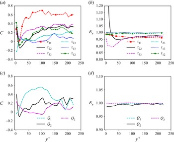
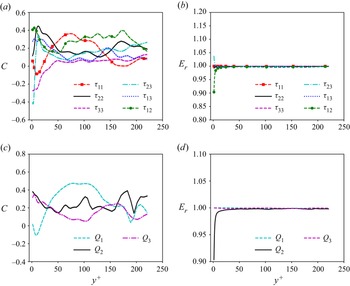
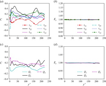
 $n_{z}=4$ in R1M15 are shown in figures 1, 2 and 3, respectively. The lighter sections of each line in figures 1, 2 and 3(a,c) represent the 95 % confidence intervals for the correlation coefficients calculated by using the Fisher transformation (Bonett & Wright Reference Bonett and Wright2000). The eddy-viscosity models assume that the SGS stress is linearly aligned with the filtered strain-rate tensor based on the Boussinesq hypothesis; similarly, the SGS heat flux is also assumed to be linearly proportional to the gradient of the resolved temperature. However, the linear alignment assumptions are unphysical and contradictory with the complicated nonlinear relations between the SGS stress and the filtered strain-rate tensor as well as between the SGS heat flux and the gradient of the filtered temperature. Therefore, it is shown that the correlation coefficients
 $C$ of the three traditional eddy-viscosity models are almost lower than 0.6, indicating that the traditional eddy-viscosity models correlate poorly with the true unclosed SGS terms (Anderson & Meneveau Reference Anderson and Meneveau1999; Da Silva & Métais Reference Da Silva and Métais2002; Xie et al. Reference Xie, Li, Ma and Wang2019a,Reference Xie, Wang, Li and Mac, Reference Xie, Yuan and Wang2020a,Reference Xie, Wang and Weinanb). These low correlations of the three traditional eddy-viscosity models can be ascribed to the unphysical linear alignment assumptions in the eddy-viscosity models. To be specific, the correlation coefficients in DSM are relatively small in the near-wall region, and slightly increase as
 $y^{+}$ increases. However, in the Vreman model and WALE model, the correlation coefficients in the near-wall region are similar to those in the far-wall region. These observations can be attributed to the reasons that the DSM cannot capture the correct behaviour in the vicinity of the wall, resulting in an extremely high damping of fluctuations near the wall, while the Vreman model and WALE model are constructed to guarantee that the dissipation is relatively small in the near-wall region. Therefore, the correlation coefficients of Vreman model and WALE model are slightly larger than those of DSM near the wall. Furthermore, it is found that the correlation coefficients of the diagonal components of the SGS stress (i.e.
 $\tau _{11}$,
 $\tau _{22}$ and
 $\tau _{33}$) are slightly larger in DSM than those in Vreman model and WALE model. This can be ascribed to the reason that the model coefficients
 $C_{I}$ of the SGS eddy viscosity
 $\mu _{I,SGS}$ are zero in the Vreman model and WALE model, while
 $C_{I}$ is dynamically solved based on the Germano identity (Moin et al. Reference Moin, Squires, Cabot and Lee1991; Lilly Reference Lilly1992; Xie et al. Reference Xie, Wang, Li, Wan and Chen2019b) in DSM. Moreover, the relative errors
 $E_{r}$ of the three traditional eddy-viscosity models are almost equal to 1.0, suggesting that the traditional eddy-viscosity models have very large errors when predicting the true unclosed SGS terms. The above observations are consistent with many previous studies (Anderson & Meneveau Reference Anderson and Meneveau1999; Da Silva & Métais Reference Da Silva and Métais2002; Xie et al. Reference Xie, Li, Ma and Wang2019a, Reference Xie, Yuan and Wang2020a,Reference Xie, Wang and Weinanb; Yuan et al. Reference Yuan, Xie and Wang2020).
(a,c) The correlation coefficients  $C$ and (b,d) the relative errors
 $E_{r}$ of DSM along the wall-normal direction in a priori test with filtered sizes
 $n_{x}=8$ and
 $n_{z}=4$ in R1M15. The lighter sections of each line in (a,c) represent the 95 % confidence intervals for the correlation coefficients.

(a,c) The correlation coefficients  $C$ and (b,d) the relative errors
 $E_{r}$ of the Vreman model along the wall-normal direction in a priori test with filtered sizes
 $n_{x}=8$ and
 $n_{z}=4$ in R1M15. The shaded areas under each line in (a,c) represent the 95 % confidence intervals for the correlation coefficients.

(a,c) The correlation coefficients  $C$ and (b,d) the relative errors
 $E_{r}$ of the WALE model along the wall-normal direction in a priori test with filtered sizes
 $n_{x}=8$ and
 $n_{z}=4$ in R1M15. The shaded areas under each line in (a,c) represent the 95 % confidence intervals for the correlation coefficients.

3. The structure and a priori test of the ANN-based nonlinear algebraic model
3.1. The original ANN-based nonlinear algebraic model
In the SGS modelling, the constitutive relation of the unclosed SGS terms can be considered as the function of the local filtered quantities, including the filtered strain-rate tensor  $\tilde {S}_{ij}$, the filtered rotation-rate tensor
 $\tilde {\varOmega }_{ij}$ and the filtered temperature gradients
 $\partial \tilde {T}/\partial x_{j}$, namely (Pope Reference Pope1975; Lund & Novikov Reference Lund and Novikov1992; Wang et al. Reference Wang, Yin, Yee and Bergstrom2007; Vollant et al. Reference Vollant, Balarac and Corre2017)
 \begin{gather} \tau _{ij}=f(\tilde{S}_{ij},\tilde{\varOmega }_{ij} ), \end{gather}
 \begin{gather} Q _{j}=f\Bigg (\tilde{S}_{ij},\tilde{\varOmega }_{ij},\frac{\partial \tilde{T}}{\partial x_{j}} \Bigg), \end{gather}
where the filtered rotation-rate tensor  $\tilde {\varOmega }_{ij}$ is given by
 \begin{equation} \tilde{\varOmega }_{ij}=\frac{1}{2}\left ( \frac{\partial \tilde{u}_{i}}{\partial x_{j}}-\frac{\partial \tilde{u}_{j}}{\partial x_{i}} \right ). \end{equation}
The SGS stress tensor  $\tau _{ij}$ can be divided into anisotropic and isotropic parts, respectively:
 $\tau _{ij}=\tau _{ij}^{A}+\tau _{ij}^{I}$, where the anisotropic part is
 $\tau _{ij}^{A}=\tau _{ij}-\tfrac {1}{3}\delta _{ij}\tau _{kk}$, and the isotropic part is
 $\tau _{ij}^{I}=\tfrac {1}{3}\delta _{ij}\tau _{kk}$.
In order to get rid of the unphysical linear alignment assumption in the traditional eddy-viscosity models, the nonlinear algebraic models of the SGS stress (Lund & Novikov Reference Lund and Novikov1992) and SGS heat flux (Vollant et al. Reference Vollant, Balarac and Corre2017) were proposed to construct the nonlinear relation between the unclosed SGS terms and the local filtered quantities.
Similar to the previous analysis of Lund & Novikov (Reference Lund and Novikov1992), the anisotropic SGS stress can be approximated as (Lund & Novikov Reference Lund and Novikov1992; Xie et al. Reference Xie, Yuan and Wang2020b)
 \begin{equation} \tau _{ij}^{A}=\varDelta ^{2}\left ( C_{1}^{A}\left \| \tilde{\boldsymbol{S}} \right \|\boldsymbol{T}_{1}^{A}+C_{2}^{A}\boldsymbol{T}_{2}^{A}+C_{3}^{A}\boldsymbol{T}_{3}^{A}+C_{4}^{A}\boldsymbol{T}_{4}^{A}+C_{5}^{A}\frac{1}{\left \| \tilde{\boldsymbol{S}} \right \|}\boldsymbol{T}_{5}^{A} \right ), \end{equation}
where
 \begin{gather} \boldsymbol{T}_{1}^{A}=\tilde{\boldsymbol{S}}-\tfrac{1}{3}\boldsymbol{I}\boldsymbol{\cdot} {\rm Tr}( \tilde{\boldsymbol{S}} ), \end{gather}
 \begin{gather} \boldsymbol{T}_{2}^{A}=\tilde{\boldsymbol{S}}\tilde{\boldsymbol{\varOmega }}-\tilde{\boldsymbol{\varOmega }}\tilde{\boldsymbol{S}}, \end{gather}
 \begin{gather} \boldsymbol{T}_{3}^{A}=\tilde{\boldsymbol{S}}^{2}-\tfrac{1}{3}\boldsymbol{I}\boldsymbol{\cdot} {\rm Tr}(\tilde{\boldsymbol{S}}^{2} ), \end{gather}
 \begin{gather} \boldsymbol{T}_{4}^{A}=\tilde{\boldsymbol{\varOmega }}^{2}-\tfrac{1}{3}\boldsymbol{I}\boldsymbol{\cdot} {\rm Tr}(\tilde{\boldsymbol{\varOmega }}^{2} ), \end{gather}
 \begin{gather} \boldsymbol{T}_{5}^{A}=\tilde{\boldsymbol{\varOmega }}\tilde{\boldsymbol{S}}^{2}-\tilde{\boldsymbol{S}}^{2}\tilde{\boldsymbol{\varOmega }}. \end{gather}
It is noted that, for brevity and simplicity of the tensorial polynomials, the matrix multiplications for the tensor contractions are expressed as
 \begin{equation} \tilde{\boldsymbol{S}}^{2}=\tilde{S}_{ik}\tilde{S}_{kj},\quad \tilde{\boldsymbol{S}}\tilde{\boldsymbol{\varOmega }}=\tilde{S}_{ik}\tilde{\varOmega }_{kj},\quad\tilde{\boldsymbol{\varOmega }}\tilde{\boldsymbol{S}}^{2}=\tilde{\varOmega }_{ik}\tilde{S}_{kl}\tilde{S}_{lj},\,{\rm Tr}(\tilde{\boldsymbol{S}}^{2} )=\tilde{S}_{ik}\tilde{S}_{ki}. \end{equation}
Furthermore, the isotropic SGS stress can be approximated as
 \begin{equation} \tau _{kk}=\varDelta ^{2}\left ( C_{0}^{I}\left \| \tilde{\boldsymbol{S}} \right \|^{2}+C_{1}^{I}\left \| \tilde{\boldsymbol{S}} \right \|\boldsymbol{T}_{1}^{I}+C_{2}^{I}\boldsymbol{T}_{2}^{I}+C_{3}^{I}\boldsymbol{T}_{3}^{I} \right ), \end{equation}
where
 \begin{gather} \boldsymbol{T}_{1}^{I}=\boldsymbol{I}\boldsymbol{\cdot} {\rm Tr} ( \tilde{\boldsymbol{S}} ), \end{gather}
 \begin{gather} \boldsymbol{T}_{2}^{I}=\boldsymbol{I}\boldsymbol{\cdot} {\rm Tr} (\tilde{\boldsymbol{S}}^{2} ), \end{gather}
 \begin{gather} \boldsymbol{T}_{3}^{I}=\boldsymbol{I}\boldsymbol{\cdot} {\rm Tr} (\tilde{\boldsymbol{\varOmega }}^{2} ). \end{gather}
Here,  $\varDelta = ( \varDelta _{x}\varDelta _{y}\varDelta _{z} )^{1/3}$ is the characteristic length scale of the grid width and
 $\| \tilde {\boldsymbol {S}} \|=\sqrt {{\rm Tr} (\tilde {\boldsymbol {S}}^{2} )}$.
It has been shown that these dimensionless model coefficients  $C_{i}^{A}$ and
 $C_{i}^{I}$ in (3.4) and (3.11) are functions of the following five invariants (Pope Reference Pope1975; Lund & Novikov Reference Lund and Novikov1992; Xie et al. Reference Xie, Yuan and Wang2020b):
 \begin{gather} \lambda _{1}\!=\! {\rm Tr}( \tilde{\boldsymbol{S}}^{2} ),\quad\lambda _{2}\!=\! {\rm Tr}( \tilde{\boldsymbol{\varOmega }}^{2} ),\quad\lambda _{3}\!=\! {\rm Tr}( \tilde{\boldsymbol{S}}^{3} ),\quad\lambda _{4}\!=\!{\rm Tr}( \tilde{\boldsymbol{\varOmega }}^{2}\tilde{\boldsymbol{S}} ),\quad\lambda _{5}={\rm Tr}( \tilde{\boldsymbol{\varOmega }}^{2}\tilde{\boldsymbol{S}}^{2} ), \end{gather}
where  $\lambda _{1}$ is the strain-rate magnitude,
 $\lambda _{2}$ is the enstrophy magnitude,
 $\lambda _{3}$ is associated with the self-amplification of the strain rate,
 $\lambda _{4}$ is the vortex stretching and
 $\lambda _{5}$ is the magnitude of the vortex stretching vector (Chamecki, Meneveau & Parlange Reference Chamecki, Meneveau and Parlange2007). Furthermore, we can reduce the above five invariants to four dimensionless ones using one or several of them appropriately in denominators (Lund & Novikov Reference Lund and Novikov1992; Chamecki et al. Reference Chamecki, Meneveau and Parlange2007; Xie et al. Reference Xie, Yuan and Wang2020b), and the four dimensionless invariants can be expressed as
 \begin{equation} d_{1}=\frac{{\rm Tr}( \tilde{\boldsymbol{\varOmega }}^{2} )}{{\rm Tr} ( \tilde{\boldsymbol{S}}^{2} )}, \quad d_{2}=\frac{{\rm Tr} ( \tilde{\boldsymbol{S}}^{3} )}{{\rm Tr} ( \tilde{\boldsymbol{S}}^{2} )^{3/2}},\quad d_{3}=\frac{{\rm Tr} ( \tilde{\boldsymbol{\varOmega }}^{2}\tilde{\boldsymbol{S}} )}{{\rm Tr} ( \tilde{\boldsymbol{S}}^{2} )^{1/2}{\rm Tr} ( \tilde{\boldsymbol{\varOmega }}^{2} )},\quad d_{4}=\frac{{\rm Tr} ( \tilde{\boldsymbol{\varOmega }}^{2}\tilde{\boldsymbol{S}}^{2} )}{{\rm Tr} ( \tilde{\boldsymbol{S}}^{2} ){\rm Tr} ( \tilde{\boldsymbol{\varOmega }}^{2} )}. \end{equation}
On the other hand, similar to the previous analysis of Vollant et al. (Reference Vollant, Balarac and Corre2017), the SGS heat flux can be approximated as
 \begin{equation} Q_{j}=\varDelta ^{2}\left (C_{1}^{Q}\left | \tilde{\boldsymbol{S}} \right |\frac{\partial \tilde{T}}{\partial x_{j}}+C_{2}^{Q}\tilde{S}_{jk}\frac{\partial \tilde{T}}{\partial x_{k}}+C_{3}^{Q}\tilde{\varOmega }_{jk}\frac{\partial \tilde{T}}{\partial x_{k}}+C_{4}^{Q}\frac{\tilde{S}_{jk}\tilde{S}_{kl}}{\left | \tilde{\boldsymbol{S}} \right |}\frac{\partial \tilde{T}}{\partial x_{l}}\right ), \end{equation}
where  $| \tilde {\boldsymbol {S}} |=\sqrt { 2\tilde {S}_{ij}\tilde {S}_{ij}}$. The model coefficients
 $C_{i}^{Q}$ in (3.17) depend on the principal invariants of tensor
 $\tilde {S}_{ij}$ and vector
 $\tilde {v}_{i}=\varDelta ^{2} | \tilde {\boldsymbol {S}} |\frac {\partial \tilde {T}}{\partial x_{i}}$, which are expressed as (Noll Reference Noll1967; Vollant et al. Reference Vollant, Balarac and Corre2017)
 \begin{gather} q_{1}=\tilde{S}_{ii},\quad q_{2}=\tilde{S}_{ij}\tilde{S}_{ji},\quad q_{3}=\tilde{S}_{ik}\tilde{S}_{kl}\tilde{S}_{li},\quad q_{4}=\tilde{v}_{i}\tilde{v}_{i},\quad q_{5}=\tilde{v}_{i}\tilde{S}_{ik}\tilde{v}_{k},\quad q_{6}=\tilde{v}_{i}\tilde{S}_{ik}\tilde{S}_{kj}\tilde{v}_{j}. \end{gather}
Similar to the DSM, the dimensionless model coefficients  $C_{i}^{A}$,
 $C_{i}^{I}$ and
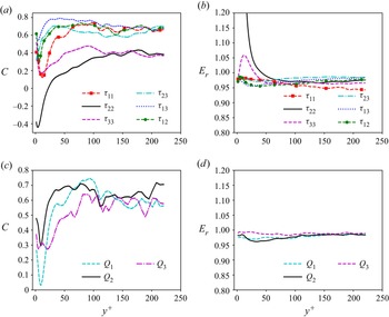
 $C_{i}^{Q}$ in (3.4), (3.11) and (3.17) respectively can also be solved dynamically based on the Germano identity (Germano et al. Reference Germano, Piomelli, Moin and Cabot1991; Lilly Reference Lilly1992; Yuan et al. Reference Yuan, Wang, Xie and Wang2022). Therefore, this original dynamic nonlinear algebraic model is named the ‘ODNA model’ for brevity. The correlation coefficients
 $C$ and the relative errors
 $E_{r}$ of the ODNA model along wall-normal direction in a priori test with filtered sizes
 $n_{x}=8$ and
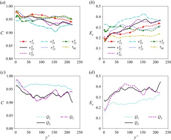
 $n_{z}=4$ in R1M15 are shown in figure 4. It is found that, in the far-wall region (
 $y^{+} > 50$), the correlation coefficients of the ODNA model are all larger than 0.4, and are significantly larger than those of the aforementioned three eddy-viscosity SGS models (DSM, Vreman and WALE). This observation indicates that the nonlinear algebraic model has a better performance than the traditional eddy-viscosity SGS models. However, the correlation coefficients of the ODNA model are pretty small near the wall, mainly due to the neglect of the anisotropy of the grid widths in wall-bounded flows. Moreover, the relative errors of the ODNA model are approximately equal to 0.98 in most components, which is only slightly smaller than the traditional eddy-viscosity SGS models.
(a,c) The correlation coefficients  $C$ and (b,d) the relative errors
 $E_{r}$ of the ODNA model along wall-normal direction in a priori test with filtered sizes
 $n_{x}=8$ and
 $n_{z}=4$ in R1M15. The lighter sections of each line in (a,c) represent the 95 % confidence intervals for the correlation coefficients.

It is shown in figure 4 that, when the dimensionless model coefficients  $C_{i}^{A}$,
 $C_{i}^{I}$ and
 $C_{i}^{Q}$ are solved dynamically based on the Germano identity (Germano et al. Reference Germano, Piomelli, Moin and Cabot1991; Lilly Reference Lilly1992; Yuan et al. Reference Yuan, Wang, Xie and Wang2022), the ODNA model cannot achieve a very good performance in a priori tests. Therefore, the dimensionless model coefficients
 $C_{i}^{A}$,
 $C_{i}^{I}$ and
 $C_{i}^{Q}$ in (3.4), (3.11) and (3.17) respectively can also be determined by the ANN method (Xie et al. Reference Xie, Yuan and Wang2020b). The schematic diagram of the ANN structure is shown in figure 5. It is shown that the ANN is composed of multiple layers and each layer has many neurons. The neurons in the
 $l$th layer receive the inputs
 $X_{j}^{l-1}$ from the
 $( l-1 )$th layer and then transmit them to the outputs
 $X_{i}^{l}$ activated by the nonlinear activation function. The transfer function from the
 $( l-1 )$th layer to the
 $l$th layer can be expressed as
 \begin{equation} X_{i}^{\left ( l \right )}=\sigma \left [ b_{i}^{\left ( l \right )}+\sum_{j}W_{ij}^{\left ( l \right )}X_{j}^{\left ( l-1 \right )} \right ], \end{equation}
where  $\sigma [ {\cdot } ]$ is the nonlinear activation function,
 $W_{ij}^{ ( l )}$ and
 $b_{i}^{ ( l )}$ are the weights and biases in the
 $l$th layer, respectively. It is noted that the ANN method is only used to generate the nonlinear relation between the input features and the model coefficients
 $C_{i}^{A}$,
 $C_{i}^{I}$ and
 $C_{i}^{Q}$. Then the generated model coefficients
 $C_{i}^{A}$,
 $C_{i}^{I}$ and
 $C_{i}^{Q}$ are multiplied with the corresponding tensor bases to get predicted values of the unclosed SGS terms
 $\tau _{ij}^{A}$,
 $\tau _{kk}$ and
 $Q_{j}$, respectively. Then the discrepancy between the predicted values of the unclosed SGS terms and the true values of the unclosed SGS terms are the loss function which is minimised during the training process. This original ANN-based nonlinear algebraic model is named the ‘OANA model’.
The schematic diagram of the ANN structure.

There are four layers of neurons ( $N_{i}:N_{h}:N_{h}:N_{o}$) between the input features and the coefficient output layer with a leaky-rectified linear unit (leaky-ReLU) activation function (Ling et al. Reference Ling, Kurzawski and Templeton2016; Xie et al. Reference Xie, Yuan and Wang2020b)
 $\sigma ( x )=\max [ -0.1x,x ]$, where
 $N_{i}$,
 $N_{h}$ and
 $N_{o}$ are the numbers of neurons of the input layer, hidden layers and coefficient output layer, respectively. It is noted that the numbers of neurons of the hidden layers
 $N_{h}$ can be arbitrarily chosen, while the numbers of the neurons of the coefficient output layer
 $N_{o}$ is a fixed number which is equal to the number of model coefficients. It is worth noting that the leaky-ReLU activation is known to perform better than the ReLU activation (Xu et al. Reference Xu, Wang, Chen and Li2015), due to the fact that the leaky-ReLU activation is capable of resolving the gradient vanishing problem of the ReLU activation. The input features, the variable of the coefficient output layer, the variable of the merge output layer and the values of
 $N_{i}$ and
 $N_{o}$ of the OANA model for the unclosed SGS terms
 $\tau _{ij}^{A}$,
 $\tau _{kk}$ and
 $Q_{j}$ are respectively listed in table 1. It is noted that, except for the invariants shown in (3.16a–d) and (3.18a–f), another feature
 $Re_{l}=\bar {\rho } ( \tilde {u}^{2}+\tilde {v}^{2}+\tilde {w}^{2} )^{1/2}h/\tilde {\mu }$ is also included to represent the local Reynolds number, and this feature
 $Re_{l}$ can introduce one of the key quantities of wall-bounded flows, the wall-normal distance from the wall
 $h$, into the input features (Yu et al. Reference Yu, Yuan, Qi, Wang, Li and Chen2022). The coefficient output layer has
 $N_{o}$ neurons and represents the model coefficients
 $C_{i}^{A}$,
 $C_{i}^{I}$ and
 $C_{i}^{Q}$ for the unclosed SGS terms
 $\tau _{ij}^{A}$,
 $\tau _{kk}$ and
 $Q_{j}$, respectively. The tensor input layer also has
 $N_{o}$ neurons for the
 $N_{o}$ tensor bases shown in (3.4), (3.11) and (3.17), respectively, where
 $N_{o}=5$ for the
 $\tau _{ij}^{A}$ term,
 $N_{o}=4$ for the
 $\tau _{kk}$ term,
 $N_{o}=4$ for the
 $Q_{j}$ term. Each model coefficient
 $C_{i}^{A}$,
 $C_{i}^{I}$ and
 $C_{i}^{Q}$ in the coefficient output layer is multiplied with the corresponding tensor bases in the tensor input layer to generate the predicted values of the unclosed SGS term
 $\tau _{ij}^{A}$,
 $\tau _{kk}$ and
 $Q_{j}$ as (3.4), (3.11) and (3.17) expressed, respectively. The differences between the predicted values and the true values of the unclosed SGS terms are minimised by the optimisation algorithm during the training process. The unclosed SGS terms
 $\tau _{ij}^{A}$,
 $\tau _{kk}$ and
 $Q_{j}$ have six, one and three components, respectively, therefore we should train ten ANNs in total.
The input features, the variable of the coefficient output layer, the variable of the merge output layer and the values of  $N_{i}$ and
 $N_{o}$ of the OANA model for the unclosed SGS terms
 $\tau _{ij}^{A}$,
 $\tau _{kk}$ and
 $Q_{j}$, respectively. Here, the input features
 $d_{1}$–
 $d_{4}$ are the invariants shown in (3.16a–d), and the input features
 $q_{1}$–
 $q_{6}$ are the invariants shown in (3.18a–f). Furthermore,
 $Re_{l}=\bar {\rho } ( \tilde {u}^{2}+\tilde {v}^{2}+\tilde {w}^{2} )^{1/2}h/\tilde {\mu }$ represents the local Reynolds number, where
 $h$ is the wall-normal distance from the wall.

The OANA model is trained with fDNS data of the turbulent channel flow case R1M15, with the filtered streamwise and spanwise sizes  $n_{x}=8$ and
 $n_{z}=4$, respectively. The input variables are rescaled by the mean and standard deviation of the input filtered variables, which can be given by
 \begin{equation} m^{{\star}}=\frac{m-\left \langle m \right \rangle_{xz}}{\sqrt{\left \langle \left ( m-\left \langle m \right \rangle _{xz}\right )^{2} \right \rangle_{xz}}}, \end{equation}
where  $m^{\star }$ represents the normalisation of the input variable
 $m$. Due to the strong anisotropy in the wall-normal direction of the wall-bounded flows, the input variables are normalised by the mean and standard deviation in the streamwise–spanwise wall-parallel plane at each wall-normal location. Furthermore, the true unclosed SGS terms
 $\tau _{ij}^{A}$,
 $\tau _{kk}$ and
 $Q_{j}$ and their corresponding tensor bases are normalised by the r.m.s. (root mean square) values of the gradient models for
 $\tau _{ij}^{A}$,
 $\tau _{kk}$ and
 $Q_{j}$ at each wall-normal location, which can be expressed as
 \begin{gather} {\tau _{ij}^{A}}^{{\star}}=\frac{\tau _{ij}^{A}}{\sqrt{\left \langle\left ({\tau _{ij}^{A}}^{GM} \right )^{2} \right \rangle_{xz}}},\quad \tau _{kk}^{{\star}}=\frac{\tau _{kk}}{\sqrt{\left \langle\left ({\tau _{kk}}^{GM} \right )^{2} \right \rangle_{xz}}},\quad Q_{j}^{{\star}}=\frac{Q_{j}}{\sqrt{\left \langle\left ({Q_{j}}^{GM} \right )^{2} \right \rangle_{xz}}}; \end{gather}
 \begin{gather} \boldsymbol{T}^{{\star}}_{\tau _{ij}^{A}}=\frac{\boldsymbol{T}_{\tau _{ij}^{A}}}{\sqrt{\left \langle\left ({\tau _{ij}^{A}}^{GM} \right )^{2} \right \rangle_{xz}}},\quad \boldsymbol{T}^{{\star}}_{\tau _{kk}}=\frac{\boldsymbol{T}_{\tau _{kk}}}{\sqrt{\left \langle\left ({\tau _{kk}}^{GM} \right )^{2} \right \rangle_{xz}}},\quad \boldsymbol{T}^{{\star}}_{Q_{j}}=\frac{\boldsymbol{T}_{Q_{j}}}{\sqrt{\left \langle\left ({Q_{j}}^{GM} \right )^{2} \right \rangle_{xz}}}, \end{gather}
where  $\boldsymbol {T}^{\star }_{\tau _{ij}^{A}}$,
 $\boldsymbol {T}^{\star }_{\tau _{kk}}$ and
 $\boldsymbol {T}^{\star }_{Q_{j}}$ are the tensor bases of the unclosed terms
 $\tau _{ij}^{A}$,
 $\tau _{kk}$ and
 $Q_{j}$ in (3.4), (3.11) and (3.17), respectively. Moreover, the gradient models
 ${\tau _{ij}^{A}}^{GM}$,
 ${\tau _{kk}}^{GM}$ and
 ${Q_{j}}^{GM}$ for
 $\tau _{ij}^{A}$,
 $\tau _{kk}$ and
 $Q_{j}$ respectively can be expressed as (Clark Reference Clark1979)
 \begin{gather} {\tau _{ij}^{A}}^{GM}=\frac{1}{12}\varDelta _{l}^{2}\frac{\partial \tilde{u}_{i}}{\partial x_{l}}\frac{\partial \tilde{u}_{j}}{\partial x_{l}}-\frac{1}{3}\delta _{ij}\frac{1}{12}\varDelta _{l}^{2}\frac{\partial \tilde{u}_{k}}{\partial x_{l}}\frac{\partial \tilde{u}_{k}}{\partial x_{l}}, \end{gather}
 \begin{gather} {\tau _{kk}}^{GM}=\frac{1}{12}\varDelta _{l}^{2}\frac{\partial \tilde{u}_{k}}{\partial x_{l}}\frac{\partial \tilde{u}_{k}}{\partial x_{l}}, \end{gather}
 \begin{gather} {Q_{j}}^{GM}=\frac{1}{12}\varDelta _{l}^{2}\frac{\partial \tilde{u}_{j}}{\partial x_{l}}\frac{\partial \tilde{T}}{\partial x_{l}}. \end{gather}
During the training process, the weights  $W_{ij}^{ ( l )}$ and biases
 $b_{i}^{ ( l )}$ are optimised to minimise the mean-squared error loss function defined as
 \begin{equation} L=\frac{1}{N_{batch}}\sum_{n=1}^{N_{batch}}\left ( f_{true}-f_{predict} \right )^{2}, \end{equation}
where  $f$ represents
 $\tau _{ij}^{A}$,
 $\tau _{kk}$ and
 $Q_{j}$ in their corresponding ANN training process. Furthermore,
 $f_{true}$ is the true unclosed SGS term (i.e.
 $\tau _{ij}^{A}$,
 $\tau _{kk}$ and
 $Q_{j}$) obtained from the fDNS data, and
 $f_{predict}$ is the predicted unclosed SGS term by the ANN. The size of the mini-batch
 $N_{batch}$ is set to be 1000.
A total of almost  $1.8\times 10^{7}$ samples of the fDNS are used for the ANN training procedure. The dataset is divided into the training, validating and testing sets to suppress parameter overfitting of the ANN: 60 % of the samples are used as the training set, 15 % of the samples are used as the validating set and 25 % of the samples are used as the testing set. Furthermore, the samples at each wall-normal location are randomly extracted to be the training, validating and testing sets. The weights of the ANN are initialised by the Glorot-uniform algorithm (Glorot & Bengio Reference Glorot and Bengio2010), and the biases are initialised to be zero. Finally, the ANN is trained by the Adam algorithm (Kingma & Ba Reference Kingma and Ba2014) to update
 $W_{ij}^{ ( l )}$ and
 $b_{i}^{ ( l )}$ for 2000 epochs with an initial learning rate of 0.001. The learning rate will further decrease by 90 % once the validated loss stops decreasing in each 10 epochs. The influences of the size of the mini-batch
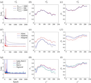
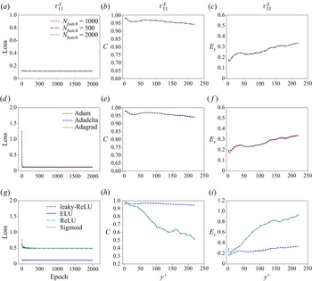
 $N_{batch}$, different optimisers and activation functions on the performance of the OANA model in a priori tests are checked in the Appendix.
We train two sets of the OANA model with different numbers of neurons of the hidden layers  $N_{h}$, and name them ‘OANA-1’ for
 $N_{h}=10$ and ‘OANA-2’ for
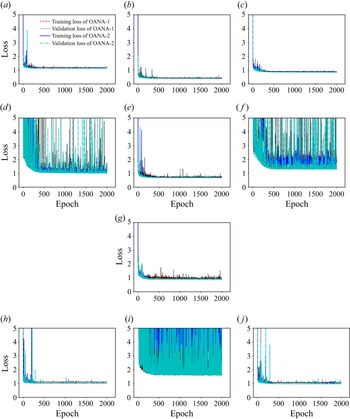
 $N_{h}=20$. The learning curves of the training and validation losses of the OANA-1 and OANA-2 models for
 $\tau _{ij}^{A}$,
 $\tau _{kk}$ and
 $Q_{j}$ are shown in figure 6. It is shown that the training and validation losses of most components decrease drastically in the initial several epochs, and then converge quickly and gradually reach stationarity. Furthermore, the learning curves of the training and validation losses are close to each other, indicating that the ANN models are well trained and remove overfitting phenomena. However, the training and validation losses of the wall-normal components (i.e.
 $\tau _{23}^{A}$,
 $\tau _{12}^{A}$,
 $Q_{2}$) oscillate drastically, although they decrease quickly in the initial several epochs. This indicates that the wall-normal components
 $\tau _{23}^{A}$,
 $\tau _{12}^{A}$ and
 $Q_{2}$ are relatively hard to train. Moreover, the weights and biases of the OANA model used in the following a priori test are obtained from the epoch where the validation losses reach the minimum values. It is also found that the training and validation losses are all pretty large, suggesting the relatively large errors of the OANA model.
The learning curves of the training and validation loss of the OANA-1 and OANA-2 models for (a)  $\tau _{11}^{A}$, (b)
 $\tau _{22}^{A}$, (c)
 $\tau _{33}^{A}$, (d)
 $\tau _{23}^{A}$, (e)
 $\tau _{13}^{A}$, (f)
 $\tau _{12}^{A}$, (g)
 $\tau _{kk}$, (h)
 $Q_{1}$, (i)
 $Q_{2}$ and (j)
 $Q_{3}$.

In order to evaluate the performance of the OANA model in an a priori test, the correlation coefficients  $C$ and the relative errors
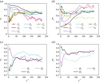
 $E_{r}$ of the OANA-2 model in the testing set along wall-normal direction are shown in figure 7. It is noted that the correlation coefficients
 $C$ and the relative errors
 $E_{r}$ of the OANA-2 model in the training set and validating set are similar to those in the testing set, therefore we only exhibit the results of the testing set to evaluate the performance of the OANA-2 model in the untrained data. It is shown that the correlation coefficients
 $C$ of most components are larger than 0.6, except for those of the components
 $\tau _{11}^{A}$ and
 $\tau _{33}^{A}$, which are approximately larger than 0.4. Even though the correlation coefficients
 $C$ of OANA-2 model are not very high, they are still significantly larger than those of the aforementioned three eddy-viscosity SGS models (DSM, Vreman and WALE), which are mostly smaller than 0.4. Furthermore, the relative errors
 $E_{r}$ are approximately equal to 0.8 in most components, which is relatively high but still much smaller than those of the aforementioned three eddy-viscosity SGS models (DSM, Vreman and WALE). On the other hand, it is also found that the OANA-2 model has significantly larger correlation coefficients than the ODNA model near the wall (
 $y^{+}<50$), while the correlation coefficients of OANA-2 model are similar to those of ODNA model far from the wall (
 $y^{+}>50$), which indicates that the ANN method can significantly enhance the correlation coefficients near the wall, while it makes a relatively small enhancement in the far-wall region compared with the dynamic method when predicting the model coefficients. Moreover, the relative errors of OANA-2 model are much smaller than those of the ODNA model, which suggests that the ANN method can significantly decrease the relative errors compared with the dynamics method. It is noted that increasing the numbers of hidden layers and neurons only gives a slight improvement of the model performance. Therefore, it is concluded that, although the OANA model has larger correlation coefficients, smaller relative errors and better performance than those of the aforementioned three eddy-viscosity SGS models (DSM, Vreman and WALE) and the ODNA model, it is still not a well-performing model.
(a,c) The correlation coefficients  $C$ and (b,d) the relative errors
 $E_{r}$ of the OANA-2 model in the testing set along wall-normal direction in a priori test with filtered sizes
 $n_{x}=8$ and
 $n_{z}=4$ in R1M15. The lighter sections of each line in (a,c) represent the 95 % confidence intervals for the correlation coefficients.

3.2. The modified ANN-based nonlinear algebraic model
The main reason for the poor performance of the OANA model and ODNA model is that they ignore the anisotropy of the grid widths in the wall-bounded flows, especially in the wall-normal direction. In the near-wall region, the wall-normal grid width  $\varDelta _{y}$ is much smaller than the streamwise grid width
 $\varDelta _{x}$ and the spanwise grid width
 $\varDelta _{z}$, which further leads to the observation that the wall-normal components
 $\tau _{23}^{A}$,
 $\tau _{12}^{A}$ and
 $Q_{2}$ have strongly oscillating training and validation losses in the OANA model. Therefore, we propose a modified version of the nonlinear algebraic model. The core idea of the modified nonlinear algebraic model can be explained as follows: the local grid widths along the streamwise, wall-normal and spanwise directions
 $\varDelta _{x}$,
 $\varDelta _{y}$ and
 $\varDelta _{z}$ are used to normalise the corresponding gradients of the flow variables (including
 $u_{i}$ and
 $T$), which can be expressed as
 \begin{equation} \frac{\partial u_{i}}{\partial x^{*}}\doteq \frac{\partial u_{i}}{\partial \left (x/\varDelta _{x} \right )},\quad \frac{\partial u_{i}}{\partial y^{*}}\doteq \frac{\partial u_{i}}{\partial (y/\varDelta _{y} )},\quad \frac{\partial u_{i}}{\partial z^{*}}\doteq \frac{\partial u_{i}}{\partial \left (z/\varDelta _{z} \right )}; \end{equation}
and
 \begin{equation} \frac{\partial T}{\partial x^{*}}\doteq \frac{\partial T}{\partial \left (x/\varDelta _{x} \right )},\quad\frac{\partial T}{\partial y^{*}}\doteq \frac{\partial T}{\partial (y/\varDelta _{y} )},\quad\frac{\partial T}{\partial z^{*}}\doteq \frac{\partial T}{\partial \left (z/\varDelta _{z} \right )}; \end{equation}
where  $x^{*}$,
 $y^{*}$ and
 $z^{*}$ are the normalised variables, which are normalised by the corresponding local grid widths
 $\varDelta _{x}$,
 $\varDelta _{y}$ and
 $\varDelta _{z}$, respectively. To be specific, the original gradients of the flow variables (including
 $u_{i}$ and
 $T$) are first calculated by the sixth-order central-difference scheme, and then multiplied by the corresponding local grid widths to generate the modified gradients in (3.27a–c) and (3.28a–c). Therefore, the modified filtered strain-rate tensor
 $\widetilde {S^{*}}_{ij}$ and modified filtered rotation-rate tensor
 $\widetilde {\varOmega ^{*}}_{ij}$ become
 \begin{gather} \widetilde{S^{*}}_{ij}=\frac{1}{2}\left ( \frac{\partial \tilde{u}_{i}}{\partial x^{*}_{j}}+\frac{\partial \tilde{u}_{j}}{\partial x^{*}_{i}} \right ), \end{gather}
 \begin{gather} \widetilde{\varOmega ^{*}}_{ij}=\frac{1}{2}\left ( \frac{\partial \tilde{u}_{i}}{\partial x^{*}_{j}}-\frac{\partial \tilde{u}_{j}}{\partial x^{*}_{i}} \right ). \end{gather}
Then, the original nonlinear algebraic model can be modified as follows. The anisotropic SGS stress can be approximated as
 \begin{equation} \tau _{ij}^{A}={\varDelta ^{*}}^{2}\left ( {C_{1}^{*}}^{A}\left \| \widetilde{\boldsymbol{S}^{*}} \right \|{\boldsymbol{T}_{1}^{*}}^{A}+{C_{2}^{*}}^{A}{\boldsymbol{T}_{2}^{*}}^{A}+{C_{3}^{*}}^{A}{\boldsymbol{T}_{3}^{*}}^{A}+{C_{4}^{*}}^{A}{\boldsymbol{T}_{4}^{*}}^{A}+{C_{5}^{*}}^{A}\frac{1}{\left \| \widetilde{\boldsymbol{S}^{*}} \right \|}{\boldsymbol{T}_{5}^{*}}^{A} \right ), \end{equation}
where
 \begin{gather} {\boldsymbol{T}_{1}^{*}}^{A}=\widetilde{\boldsymbol{S}^{*}}-\frac{1}{3}\boldsymbol{I}\boldsymbol{\cdot} {\rm Tr}\left ( \widetilde{\boldsymbol{S}^{*}} \right ), \end{gather}
 \begin{gather} {\boldsymbol{T}_{2}^{*}}^{A}=\widetilde{\boldsymbol{S}^{*}}\widetilde{\boldsymbol{\varOmega }^{*}}-\widetilde{\boldsymbol{\varOmega }^{*}}\widetilde{\boldsymbol{S}^{*}}, \end{gather}
 \begin{gather} {\boldsymbol{T}_{3}^{*}}^{A}=\widetilde{\boldsymbol{S}^{*}}^{2}-\frac{1}{3}\boldsymbol{I}\boldsymbol{\cdot} {\rm Tr}\left (\widetilde{\boldsymbol{S}^{*}}^{2} \right ), \end{gather}
 \begin{gather} {\boldsymbol{T}_{4}^{*}}^{A}=\widetilde{\boldsymbol{\varOmega }^{*}}^{2}-\frac{1}{3}\boldsymbol{I}\boldsymbol{\cdot} {\rm Tr}\left (\widetilde{\boldsymbol{\varOmega }^{*}}^{2} \right ), \end{gather}
 \begin{gather} {\boldsymbol{T}_{5}^{*}}^{A}=\widetilde{\boldsymbol{\varOmega }^{*}}\widetilde{\boldsymbol{S}^{*}}^{2}-\widetilde{\boldsymbol{S}^{*}}^{2}\widetilde{\boldsymbol{\varOmega }^{*}}. \end{gather}
The isotropic SGS stress can be approximated as
 \begin{equation} \tau _{kk}={\varDelta ^{*}}^{2}\left ( {C_{0}^{*}}^{I}\left \| \widetilde{\boldsymbol{S}^{*}} \right \|^{2}+{C_{1}^{*}}^{I}\left \| \widetilde{\boldsymbol{S}^{*}} \right \|{\boldsymbol{T}_{1}^{*}}^{I}+{C_{2}^{*}}^{I}{\boldsymbol{T}_{2}^{*}}^{I}+{C_{3}^{*}}^{I}{\boldsymbol{T}_{3}^{*}}^{I} \right ), \end{equation}
where
 \begin{gather} {\boldsymbol{T}_{1}^{*}}^{I}=\boldsymbol{I}\boldsymbol{\cdot} {\rm Tr}\left ( \widetilde{\boldsymbol{S}^{*}} \right ), \end{gather}
 \begin{gather} {\boldsymbol{T}_{2}^{*}}^{I}=\boldsymbol{I}\boldsymbol{\cdot} {\rm Tr}\left (\widetilde{\boldsymbol{S}^{*}}^{2} \right ), \end{gather}
 \begin{gather} {\boldsymbol{T}_{3}^{*}}^{I}=\boldsymbol{I}\boldsymbol{\cdot} {\rm Tr}\left (\widetilde{\boldsymbol{\varOmega }^{*}}^{2} \right ). \end{gather}
Here,  $\varDelta ^{*}=1$ is the normalised characteristic length scale and
 $\| \widetilde {\boldsymbol {S}^{*}} \|=\sqrt {{\rm Tr} (\widetilde {\boldsymbol {S}^{*}}^{2} )}$.
Moreover, the modified model coefficients  ${C_{i}^{*}}^{A}$ and
 ${C_{i}^{*}}^{I}$ in (3.31) and (3.37) are functions of the modified four dimensionless invariants, which can be expressed as
 \begin{equation} \left. \begin{aligned} d_{1}^{*} & =\frac{{\rm Tr}\left ( \widetilde{\boldsymbol{\varOmega }^{*}}^{2} \right )}{{\rm Tr}\left ( \widetilde{\boldsymbol{S}^{*}}^{2} \right )},\quad d_{2}^{*}=\frac{{\rm Tr}\left ( \widetilde{\boldsymbol{S}^{*}}^{3} \right )}{{\rm Tr}\left ( \widetilde{\boldsymbol{S}^{*}}^{2} \right )^{3/2}}, \\ d_{3}^{*} & =\frac{{\rm Tr}\left ( \widetilde{\boldsymbol{\varOmega }^{*}}^{2}\widetilde{\boldsymbol{S}^{*}} \right )}{{\rm Tr}\left ( \widetilde{\boldsymbol{S}^{*}}^{2} \right )^{1/2}{\rm Tr}\left ( \widetilde{\boldsymbol{\varOmega }^{*}}^{2} \right )},\quad d_{4}^{*}=\frac{{\rm Tr}\left ( \widetilde{\boldsymbol{\varOmega }^{*}}^{2}\widetilde{\boldsymbol{S}^{*}}^{2} \right )}{{\rm Tr}\left ( \widetilde{\boldsymbol{S}^{*}}^{2} \right ){\rm Tr}\left ( \widetilde{\boldsymbol{\varOmega }^{*}}^{2} \right )}. \end{aligned} \right\} \end{equation}
Similarly, the SGS heat flux can be approximated as
 \begin{equation} Q_{j}={\varDelta ^{*}}^{2}\left ({C_{1}^{*}}^{Q}\left | \widetilde{\boldsymbol{S}^{*}} \right |\frac{\partial \tilde{T}}{\partial x^{*}_{j}}+{C_{2}^{*}}^{Q}\widetilde{S^{*}}_{jk}\frac{\partial \tilde{T}}{\partial x^{*}_{k}}+{C_{3}^{*}}^{Q}\widetilde{\varOmega ^{*}}_{jk}\frac{\partial \tilde{T}}{\partial x^{*}_{k}}+{C_{4}^{*}}^{Q}\frac{\widetilde{S^{*}}_{jk}\widetilde{S^{*}}_{kl}}{\left | \widetilde{\boldsymbol{S}^{*}} \right |}\frac{\partial \tilde{T}}{\partial x^{*}_{l}}\right ), \end{equation}
where  $| \widetilde {\boldsymbol {S}^{*}} |=\sqrt { 2\widetilde {S^{*}}_{ij}\widetilde {S^{*}}_{ij}}$. The model coefficients
 ${C_{i}^{*}}^{Q}$ in (3.42) depend on the principal invariants of tensor
 $\widetilde {S^{*}}_{ij}$ and vector
 $\widetilde {v^{*}}_{i}={\varDelta ^{*}}^{2} | \widetilde {\boldsymbol {S}^{*}} |({\partial \tilde {T}}/{\partial x^{*}_{i}})$, which are written as
 \begin{equation} \left. \begin{aligned} q_{1}^{*} & =\widetilde{S^{*}}_{ii},\quad q_{2}^{*}=\widetilde{S^{*}}_{ij}\widetilde{S^{*}}_{ji}, \quad q_{3}^{*}=\widetilde{S^{*}}_{ik}\widetilde{S^{*}}_{kl}\widetilde{S^{*}}_{li},\\ q_{4}^{*} & =\widetilde{v^{*}}_{i}\widetilde{v^{*}}_{i}, \quad q_{5}^{*}=\widetilde{v^{*}}_{i}\widetilde{S^{*}}_{ik}\widetilde{v^{*}}_{k}, \quad q_{6}^{*}=\widetilde{v^{*}}_{i}\widetilde{S^{*}}_{ik}\widetilde{S^{*}}_{kj} \widetilde{v^{*}}_{j}. \end{aligned} \right\} \end{equation}
Similar to the ODNA model, the modified dimensionless model coefficients  ${C_{i}^{*}}^{A}$,
 ${C_{i}^{*}}^{I}$ and
 ${C_{i}^{*}}^{Q}$ in (3.31), (3.37) and (3.42), respectively, can also be solved dynamically based on the Germano identity (Germano et al. Reference Germano, Piomelli, Moin and Cabot1991; Lilly Reference Lilly1992; Yuan et al. Reference Yuan, Wang, Xie and Wang2022). Therefore, this modified dynamic nonlinear algebraic model is named the ‘MDNA model’. The correlation coefficients
 $C$ and the relative errors
 $E_{r}$ of the MDNA model along the wall-normal direction in a priori tests with filtered sizes
 $n_{x}=8$ and
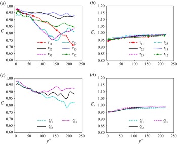
 $n_{z}=4$ in R1M15 are shown in figure 8. It is found that, compared with the correlation coefficients of the ODNA model in figure 4(a,c), the correlation coefficients of the MDNA model have significantly larger values than those of the ODNA model. The enhancement is large in the near-wall region (
 $y^{+}<50$) where the anisotropy of the grid widths is significantly strong. As
 $y^{+}$ further increases, the enhancement of the MDNA model becomes weaker, mainly due to the fact that the anisotropy of the grid widths also becomes weaker. These observations indicate that the above modification of using the local grid widths along each direction to normalise the corresponding gradients of the flow variables can significantly enhance the correlation coefficients of the dynamic nonlinear algebraic model, especially in the near-wall region. Moreover, the relative errors of the MDNA model are close to 0.95, which are slightly smaller than those of the ODNA model. This observation suggests that the above modification can slightly decrease the relative errors of the dynamic nonlinear algebraic model.
(a,c) The correlation coefficients  $C$ and (b,d) the relative errors
 $E_{r}$ of MDNA model along the wall-normal direction in a priori tests with filtered sizes
 $n_{x}=8$ and
 $n_{z}=4$ in R1M15. The lighter sections of each line in (a,c) represent the 95 % confidence intervals for the correlation coefficients.

It is shown in figure 8 that the MDNA model has a better performance than the eddy-viscosity models (DSM, Vreman and WALE) and the ODNA model, while has a similar performance to the OANA model. It is found in figures 4 and 7 that the ANN-based model has a better performance than the dynamic model. Therefore, it can be speculated that the ANN-based version of the modified nonlinear algebraic model will have a better performance. Similar to the OANA model, the modified dimensionless model coefficients  ${C_{i}^{*}}^{A}$,
 ${C_{i}^{*}}^{I}$ and
 ${C_{i}^{*}}^{Q}$ in (3.31), (3.37) and (3.42), respectively, can be determined by the ANN method, therefore the modified ANN-based nonlinear algebraic model is named the ‘MANA model’. The ANN schematic, parameter setting of the ANN and the training process of the MANA model are all the same as those in OANA model shown in § 3.1, except for that the input features are changed to the corresponding invariants, which are shown in table 2. It is noted that the MANA model considers the anisotropy of the grid widths in wall-bounded flows, and it is expected that the MANA model will have a better performance in the a priori and a posteriori tests. The influences of the size of the mini-batch
 $N_{batch}$, different optimisers and activation functions on the performance of the MANA model in a priori test are checked in the Appendix.
The input features, the variable of the coefficient output layer, the variable of the merge output layer and the values of  $N_{i}$ and
 $N_{o}$ of the MANA model for the unclosed SGS terms
 $\tau _{ij}^{A}$,
 $\tau _{kk}$ and
 $Q_{j}$, respectively. Here, the input features
 $d_{1}^{*}$–
 $d_{4}^{*}$ are the invariants shown in (3.41), and the input features
 $q_{1}^{*}$–
 $q_{6}^{*}$ are the invariants shown in (3.43).

We train three sets of MANA model with different numbers of neurons of the hidden layers  $N_{h}$, and name them ‘MANA-1’ for
 $N_{h}=10$, ‘MANA-2’ for
 $N_{h}=20$ and ‘MANA-3’ for
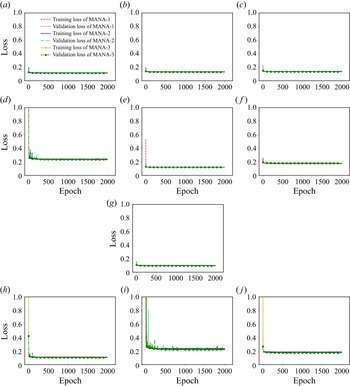
 $N_{h}=40$. The learning curves of the training and validation losses of the MANA-1, MANA-2 and MANA-3 models for
 $\tau _{ij}^{A}$,
 $\tau _{kk}$ and
 $Q_{j}$ are shown in figure 9. It is found that the training and validation losses are close to each other, and converge well, which indicates that the MANA models are well trained and avoid overfitting phenomena. Furthermore, the strong oscillation phenomena observed in the training and validation losses of the wall-normal components
 $\tau _{23}^{A}$,
 $\tau _{12}^{A}$ and
 $Q_{2}$ of OANA model (figure 6) disappear in the validation losses of the MANA model, which indicates that the above modification in the MANA model can alleviate the effect of the anisotropy of the grid widths in wall-bounded flows. The weights and biases of the MANA model used in the following a priori test are acquired from the epoch where the validation losses reach the minimum values. It is also found that the training and validation losses slightly decrease as the number of neurons of the hidden layers increases, indicating a slightly better performance of the MANA model with a larger number of hidden layer neurons.
The learning curves of the training and validation losses of the MANA-1, MANA-2 and MANA-3 models for (a)  $\tau _{11}^{A}$, (b)
 $\tau _{22}^{A}$, (c)
 $\tau _{33}^{A}$, (d)
 $\tau _{23}^{A}$, (e)
 $\tau _{13}^{A}$, (f)
 $\tau _{12}^{A}$, (g)
 $\tau _{kk}$, (h)
 $Q_{1}$, (i)
 $Q_{2}$ and (j)
 $Q_{3}$.

In order to explicitly evaluate the performance of the MANA model in a priori tests, the correlation coefficients  $C$ and the relative errors
 $E_{r}$ of the MANA-1 model in the testing set along the wall-normal direction are shown in figure 10. It is found that the correlation coefficients of
 $\tau _{ij}^{A}$,
 $\tau _{kk}$ and
 $Q_{j}$ in the MANA-1 model are all larger than 0.91, which are much higher than the ODNA model, OANA model, MDNA model and the three traditional eddy-viscosity models. Furthermore, the relative errors in the MANA-1 model are all smaller than 0.4, which are much smaller than the ODNA model, OANA model, MDNA model and the three traditional eddy-viscosity models. These observations indicate that the MANA model has a much better performance than the ODNA model, OANA model, MDNA model and the three traditional eddy-viscosity models in a priori tests. Furthermore, in order to examine the influence of the numbers of hidden layer neurons, the correlation coefficients
 $C$ and the relative errors
 $E_{r}$ of
 $\tau _{11}^{A}$ and
 $Q_{1}$ are chosen as representatives to compare the performances of the MANA-1, MANA-2 and MANA-3 models in figure 11. It is found the numbers of hidden layer neurons have little influence on the performance of the MANA model in a priori tests. Therefore, considering the computational cost of the MANA model in a posteriori tests, we use the MANA-1 model with
 $N_{h}=10$ as the final MANA model in a posteriori tests. The weights and biases of the MANA model used in the a posteriori tests are given in the supplementary material available at https://doi.org/10.1017/jfm.2023.179.
(a,c) The correlation coefficients  $C$ and (b,d) the relative errors
 $E_{r}$ of the MANA-1 model in the testing set along the wall-normal direction in a priori test with filtered sizes
 $n_{x}=8$ and
 $n_{z}=4$ in R1M15. The shaded areas under each line in (a,c) represent the 95 % confidence intervals for the correlation coefficients.

(a,b) The correlation coefficients  $C$ and the relative errors
 $E_{r}$ of
 $\tau _{11}^{A}$ in the MANA-1, MANA-2 and MANA-3 models in the testing set along the wall-normal direction. (c,d) The correlation coefficients
 $C$ and the relative errors
 $E_{r}$ of
 $Q_{1}$ in the MANA-1, MANA-2 and MANA-3 models in the testing set along the wall-normal direction.

The SGS flux of the kinetic energy can be defined as  $\varPi _{\tau }=-\tau _{ij}\partial \tilde {u}_{i}/\partial x_{j}$, which represents the energy transfer rate of the kinetic energy from the large scales to the small scales (Eyink Reference Eyink2005; Aluie & Eyink Reference Aluie and Eyink2009; Eyink & Aluie Reference Eyink and Aluie2009; Wang et al. Reference Wang, Wan, Chen and Chen2018a; Xu et al. Reference Xu, Wang, Wan, Yu, Li and Chen2021b); similarly, the SGS flux of the temperature variance can be written as
 $\varPi _{Q}=-Q_{j}\partial \tilde {T}/\partial x_{j}$, which indicates the energy transfer rate of the temperature variance from the large scales to the small scales (Jiménez et al. Reference Jiménez, Ducros, Cuenot and Béedat2001; Vollant et al. Reference Vollant, Balarac and Corre2017). Furthermore, the positive values of the SGS fluxes of the kinetic energy and the temperature variance suggest the direct energy transfer from the large scales to the small scales, while the negative values represent the inverse energy transfer from the small scales to the large scales (Eyink Reference Eyink2005; Aluie & Eyink Reference Aluie and Eyink2009; Eyink & Aluie Reference Eyink and Aluie2009; Wang et al. Reference Wang, Wan, Chen and Chen2018a; Xu et al. Reference Xu, Wang, Wan, Yu, Li and Chen2021b). The normalised SGS fluxes of the kinetic energy and the temperature variance can be expressed as
 $\varPi _{\tau }^{+}= (-\tau _{ij}\partial \tilde {u}_{i}/\partial x_{j} )/ ( u_{\tau }^{3}/\delta _{\nu } )$ and
 $\varPi _{Q}^{+}= (-Q_{j}\partial \tilde {T}/\partial x_{j} )/ ( u_{\tau }T_{w}^{2}/\delta _{\nu } )$, respectively. The streamwise–spanwise averages of the normalised SGS fluxes of the kinetic energy and the temperature variance
 $\langle \varPi _{\tau }^{+} \rangle _{xz}$ and
 $\langle \varPi _{Q}^{+} \rangle _{xz}$ along the wall-normal direction for the fDNS, Vreman, DSM, WALE, MDNA and MANA models in the a priori tests are shown in figure 12. It is shown that the traditional eddy-viscosity models (Vreman, DSM and WALE) and the dynamic nonlinear algebraic model (MDNA) significantly underestimate the mean normalised SGS fluxes of the kinetic energy and the temperature variance
 $\langle \varPi _{\tau }^{+} \rangle _{xz}$ and
 $\langle \varPi _{Q}^{+} \rangle _{xz}$, while the
 $\langle \varPi _{\tau }^{+} \rangle _{xz}$ and
 $\langle \varPi _{Q}^{+} \rangle _{xz}$ profiles of the MANA model almost collapse to those of the fDNS result, which indicates that the MANA model has a much better performance in predicting the mean normalised SGS fluxes of the kinetic energy and the temperature variance compared with the traditional eddy-viscosity models and the dynamic nonlinear algebraic model (MDNA) in a priori tests.
The streamwise–spanwise averages of the normalised SGS fluxes of the kinetic energy and the temperature variance (a)  $\langle \varPi _{\tau }^{+} \rangle _{xz}$ and (b)
 $\langle \varPi _{Q}^{+} \rangle _{xz}$ along the wall-normal direction for the fDNS, Vreman, DSM, WALE, MDNA and MANA models in the a priori test.

3.3. Discussion about the performance of different models
It is shown that the traditional eddy-viscosity models (DSM, Vreman and WALE) have poor performances in a priori tests, which can be ascribed to the unphysical assumption that the SGS stress and SGS heat flux are linearly aligned with the filtered strain-rate tensor and the gradient of the filtered temperature, respectively (Anderson & Meneveau Reference Anderson and Meneveau1999; Da Silva & Métais Reference Da Silva and Métais2002; Xie et al. Reference Xie, Li, Ma and Wang2019a,Reference Xie, Wang, Li and Mac, Reference Xie, Yuan and Wang2020a,Reference Xie, Wang and Weinanb). These issues can be addressed by the nonlinear algebraic models. It is found that the ODNA model has larger correlations and smaller relative errors than the traditional eddy-viscosity models (DSM, Vreman and WALE), indicating that the nonlinear algebraic model has a better performance than the eddy-viscosity models (DSM, Vreman and WALE). However, the ODNA model ignores the anisotropy of the grid widths in wall-bounded flows, especially in the wall-normal direction. Therefore, an innovative modification is applied on the invariants and the tensor bases of the nonlinear algebraic models through using the local grid widths along each direction to normalise the corresponding gradients of the flow variables. After applying this modification, the correlation coefficients of the MDNA model are significantly enhanced compared with those of the ODNA model, especially in the near-wall region. The relative errors of the MDNA model are also smaller than those of the ODNA model. When the model coefficients are estimated by the ANN method rather than the dynamic method, the model performance in a priori tests is significantly enhanced. Therefore, it is concluded that the nonlinear algebraic expressions of the model, the innovative modification of the expressions of the invariants and tensor bases and the model coefficients estimated by the ANN method all make significant contributions to the much better performance of the MANA model in a priori tests.
4. The a posteriori test of the MANA model
4.1. Application in the compressible turbulent channel flow with untrained grid resolution
Initially, the performance of the proposed MANA model is tested in the compressible turbulent channel flow case R1M15 with an untrained grid resolution. The filtered Navier–Stokes equations (2.1), (2.8), (2.9), (2.4) are solved by a high-order finite-difference solver in Cartesian coordinates: a sixth-order central-difference scheme is applied for the discretisation of both the convective and viscous terms, and the LES equations are temporally integrated by the third-order Runge–Kutta scheme (Shu & Osher Reference Shu and Osher1988). Similar to the grid setting in Jiang et al. (Reference Jiang, Xiao, Shi and Chen2013), the grid resolution of  $64\times 65\times 64$ and streamwise and spanwise filtered sizes
 $n_{x}=6$ and
 $n_{z}=2$ are used for LES of compressible turbulent channel flow using the MANA model, implicit large-eddy simulation (ILES) method, DSM, Vreman model and WALE model. It is noted that, when the grid numbers in statistically homogeneous directions are small, it is found that the MDNA model is sometimes unstable in a posteriori tests. Moreover, the MDNA model is much computationally expensive, almost 2.54 times the cost of DSM when simulating the same 1000 steps. Therefore, the performance of the MDNA model is not exhibited in a posteriori tests. The streamwise and spanwise filtered sizes in the a posteriori tests are different from those in the training process, where
 $n_{x}=8$ and
 $n_{z}=4$ are used, respectively. The details of the grid settings of the DNS and LES are listed in table 3. Furthermore, the computational cost of the MANA model is compared with the traditional eddy-viscosity models and ILES. The computational times for simulating the same 1000 steps are compared and listed in table 4, where the ratios of computational time in all five LES models are shown and the computational time is normalised by that of DSM. It is found that the dynamic model (DSM) is much more time consuming than the constant coefficient models (Vreman, WALE). However, the proposed MANA model is computationally much cheaper than DSM, which is also much cheaper than the other ANN-based models proposed previously in Park & Choi (Reference Park and Choi2021), Wang et al. (Reference Wang, Luo, Li, Tan and Fan2018b), Yuan et al. (Reference Yuan, Xie and Wang2020), Xie et al. (Reference Xie, Wang, Li and Ma2019c) and Xie et al. (Reference Xie, Wang and Weinan2020a).
The details of the grid settings of the DNS, ILES, Vreman model, DSM, WALE model and MANA model in the compressible channel flow case R1M15 with  $Re=3000$ and
 $M=1.5$. Here,
 $N_{x}$,
 $N_{y}$ and
 $N_{z}$ are the grid resolutions in the streamwise, wall-normal and spanwise directions, respectively.

Ratios of computational time for simulating the same 1000 steps for all five LES models. The computational time is normalised by that of DSM. The simulations are testing on 80 2.40 GHz Intel Xeon Gold 6148 CPUs. The computational time of DSM is approximately 15.4 s.

The van Driest transformed velocity,  $U_{vd}^{+}$, is defined as
 \begin{equation} U_{vd}^{+}=\int_{0}^{U^{+}}\left ( \left \langle \bar{\rho } \right \rangle_{xz}/\left \langle \bar{\rho }_{w} \right \rangle_{xz} \right )^{1/2}\,{\rm d}U^{+}, \end{equation}
where  $U^{+}= \langle \tilde {u} \rangle _{xz}/u_{\tau }$. The van Driest transformed velocity
 $U_{vd}^{+}$ and the normalised mean temperature profile
 $\langle \tilde {T} \rangle _{xz}/T_{w}$ along the wall-normal direction for fDNS and LES with different SGS models in R1M15 are plotted in figure 13. It is noted that the fDNS results in the R1M15 case are calculated by applying the top-hat filter with the streamwise and spanwise filtered sizes
 $n_{x}=6$ and
 $n_{z}=2$ to the DNS flow fields. It is shown in figure 13(a) that, in the viscous sublayer (
 $y^{+}<5$), the van Driest transformed velocity
 $U_{vd}^{+}$ increases linearly with
 $y^{+}$. Furthermore, the results of all SGS models collapse to the fDNS result in the viscous sublayer and the lower part of the buffer layer where
 $y^{+}<10$. In the log-law region, the
 $U_{vd}^{+}$ profile of the MANA model is fully consistent with that of the fDNS result. However, the
 $U_{vd}^{+}$ profiles of the traditional eddy-viscosity models (Vreman, DSM and WALE) are significantly larger than that of the fDNS result, and the
 $U_{vd}^{+}$ profile of ILES is slightly lower than that of the fDNS result. The above observations indicate that the MANA model provides the proper SGS dissipation, while the traditional eddy-viscosity models give excessive SGS dissipation, and the ILES lacks SGS dissipation, consistent with previous studies on LES of isotropic turbulence and turbulent channel flow (Xie et al. Reference Xie, Li, Ma and Wang2019a,Reference Xie, Wang, Li and Mac; Yu et al. Reference Yu, Yuan, Qi, Wang, Li and Chen2022).
(a) The van Driest transformed velocity  $U_{vd}^{+}$ and (b) the normalised mean temperature profile
 $\langle \tilde {T} \rangle _{xz}/T_{w}$ along the wall-normal direction for fDNS and LES with different SGS models in R1M15. It is noted that the fDNS results in the R1M15 case are calculated by applying the top-hat filter with the streamwise and spanwise filtered sizes
 $n_{x}=6$ and
 $n_{z}=2$ to the DNS flow fields.

It is shown in figure 13(b) that all LES results collapse to the mean temperature profile of the fDNS result in most regions of the channel, except for some regions in the centre of the channel. It is found that the mean temperature profiles of the traditional eddy-viscosity models in the centre of the channel are slightly larger than that of the fDNS result, while the mean temperature profile of the MANA model is fully consistent with that of the fDNS result.
The normalised r.m.s. values of the resolved fluctuating velocities are defined as  $\tilde {u}_{i,rms}^{+}= \langle (\tilde {u}_{i}- \langle \tilde {u}_{i} \rangle _{xz} )^{2} \rangle _{xz}^{1/2}/u_{\tau }$, which represent the resolved turbulence intensities. Furthermore,
 $\tilde {R}_{uv}^{+}= \langle ( \tilde {u}- \langle \tilde {u} \rangle _{xz} ) ( \tilde {v}- \langle \tilde {v} \rangle _{xz} ) \rangle _{xz}/u_{\tau }^{2}$ represents the normalised resolved Reynolds shear stress. The normalised r.m.s. values of the resolved fluctuating velocities
 $\tilde {u}_{i,rms}^{+}$ and the normalised resolved Reynolds shear stress
 $\tilde {R}_{uv}^{+}$ along the wall-normal direction for fDNS and LES with different SGS models in R1M15 are shown in figure 14. In figure 14(a), it is found that the ILES and the traditional eddy-viscosity models including Vreman, DSM and WALE, exhibit larger turbulence intensities than that of the fDNS result, while the
 $\tilde {u}_{rms}^{+}$ profile of the proposed MANA model fully collapses to that of the fDNS result. Similarly, the
 $\tilde {v}_{rms}^{+}$,
 $\tilde {w}_{rms}^{+}$ and
 $\tilde {R}_{uv}^{+}$ profiles of ILES, Vreman, DSM and WALE in figure 14(b–d) exhibit significant deviations from those of the fDNS result, where the peak values and the wall-normal locations of the peak values are much larger in ILES and the traditional eddy-viscosity models. However, the
 $\tilde {v}_{rms}^{+}$,
 $\tilde {w}_{rms}^{+}$ and
 $\tilde {R}_{uv}^{+}$ profiles of the MANA model are fully consistent with those of the fDNS result. To sum up, The MANA model can predict the resolved turbulent intensities and resolved Reynolds shear stress accurately and exhibits a much better performance than the ILES and the traditional eddy-viscosity models. In particular, the peak values and the locations of the peak values of the resolved turbulent intensities and resolved Reynolds shear stress are well predicted in the MANA model, while larger peak values and peak value locations further away from the wall for the resolved turbulent intensities are observed in the ILES and the traditional eddy-viscosity models.
The normalised r.m.s. values of the resolved fluctuating velocities and the normalised resolved Reynolds shear stress along the wall-normal direction for fDNS and LES with different SGS models in R1M15. (a) The streamwise resolved fluctuating velocities  $\tilde {u}_{rms}^{+}$, (b) the wall-normal resolved fluctuating velocities
 $\tilde {v}_{rms}^{+}$, (c) the spanwise resolved fluctuating velocities
 $\tilde {w}_{rms}^{+}$ and (d) the resolved Reynolds shear stress
 $\tilde {R}_{uv}^{+}$.

The visualisations of the instantaneous vortical structures based on the  $Q$-criterion (Hunt et al. Reference Hunt, Wray and Moin1988) for fDNS and LES with different SGS models in R1M15 are shown in figure 15. The structures are coloured by the wall-normal distance
 $h$, and the isosurfaces of the instantaneous vortical structures represent
 $Q=0.4$. It is shown in figure 15(a) that the vortical structures exhibit abundant long tube-like structures in the fDNS result, and the vortical structures near the wall are much thinner and longer than those far from the wall, mainly due to the strong mean shear near the wall. Furthermore, the vortical structures predicted by all SGS models are much sparser than those in the fDNS result, which arises from the sparser grid resolutions in the LES with different SGS models. Among the LES models, the MANA model exhibits more small-scale structures, while other LES models show fatter and longer tube-like structures, which indicates that the MANA model predicts more small-scale turbulent fluctuations. Accordingly, the above observations indicate that the MANA model is better than the other LES models in accurately predicting the small-scale turbulent structures.
Visualisation of the instantaneous vortical structures based on the  $Q$-criterion (Hunt, Wray & Moin Reference Hunt, Wray and Moin1988) in the (a) fDNS, (b) ILES, (c) Vreman, (d) DSM, (e) WALE and (f) MANA models. The structures are coloured by the wall-normal distance
 $h$, and the isosurfaces of the instantaneous vortical structures represent
 $Q=0.4$. It is noted that the fDNS result is generated by applying streamwise and spanwise filtering with filter sizes
 $n_{x}=6$ and
 $n_{z}=2$ to the DNS flow fields; however, the grid resolution remains as
 $384\times 193\times 128$.

The normalised r.m.s. value of the resolved fluctuating temperature is defined as  $\tilde {T}_{rms}^{+}= \langle (\tilde {T}- \langle \tilde {T} \rangle _{xz} )^{2} \rangle _{xz}^{1/2}/T_{w}$, and the normalised resolved streamwise Reynolds heat flux is defined as
 $\tilde {R}_{uT}^{+}= \langle ( \tilde {u}- \langle \tilde {u} \rangle _{xz} ) ( \tilde {T}- \langle \tilde {T} \rangle _{xz} ) \rangle _{xz}/ (u_{\tau }T_{w} )$. The normalised r.m.s. values of the resolved fluctuating temperature
 $\tilde {T}_{rms}^{+}$ and the normalised resolved streamwise Reynolds heat flux
 $\tilde {R}_{uT}^{+}$ along the wall-normal direction from fDNS and LES with different SGS models in R1M15 are shown in figure 16. It is shown that
 $\tilde {T}_{rms}^{+}$ and
 $\tilde {R}_{uT}^{+}$ in the ILES and the traditional eddy-viscosity models are quite close to the fDNS results, except for much larger peak values of
 $\tilde {T}_{rms}^{+}$ and
 $\tilde {R}_{uT}^{+}$. However, the
 $\tilde {T}_{rms}^{+}$ and
 $\tilde {R}_{uT}^{+}$ profiles in the MANA model perfectly collapse to those in the fDNS fields, indicating the accurate predictions of the MANA model for the thermodynamic statistics.
(a) The normalised r.m.s. values of the resolved fluctuating temperature  $\tilde {T}_{rms}^{+}$ and (b) the normalised resolved streamwise Reynolds heat flux
 $\tilde {R}_{uT}^{+}$ along the wall-normal direction from fDNS and LES with different SGS models in R1M15.

The streamwise–spanwise averages of the normalised SGS fluxes of the kinetic energy and the temperature variance  $\langle \varPi _{\tau }^{+} \rangle _{xz}$ and
 $\langle \varPi _{Q}^{+} \rangle _{xz}$ along the wall-normal direction for the fDNS, ILES, Vreman, DSM, WALE and MANA models in a posteriori tests in R1M15 are depicted in figure 17. The ILES is the LES with no SGS model, therefore the normalised SGS fluxes of the kinetic energy and the temperature variance
 $\langle \varPi _{\tau }^{+} \rangle _{xz}$ and
 $\langle \varPi _{Q}^{+} \rangle _{xz}$ are zero along the wall-normal direction. The Vreman and WALE models significantly underestimate the mean SGS fluxes of the kinetic energy and the temperature variance, while the DSM strongly overestimates the mean kinetic energy flux and underestimates the mean flux of the temperature variance. On the contrary, the MANA model accurately predicts the kinetic energy and the temperature variance transfer rate along the wall-normal direction, except for slightly larger values in the buffer layer. Furthermore, the instantaneous wall-parallel contour of the normalised SGS fluxes of the kinetic energy and the temperature variance
 $\varPi _{\tau }^{+}$ and
 $\varPi _{Q}^{+}$ for fDNS and LES with different SGS models at
 $y^{+}=15$ in a posteriori tests in R1M15 are shown in figures 18 and 19, respectively. It is found in figures 18 and 19 that most regions exhibit positive values of
 $\varPi _{\tau }^{+}$ and
 $\varPi _{Q}^{+}$, indicating that the compressible turbulent channel flow is dominated by the direct transfer of the kinetic energy and the temperature variance from large scales to small scales. However, the negative values of
 $\varPi _{\tau }^{+}$ and
 $\varPi _{Q}^{+}$ also appear in some regions, suggesting that the inverse transfer of the kinetic energy and the temperature variance from small scales to large scales also exist in the compressible turbulent channel flow. The above observations are consistent with those in compressible isotropic turbulence and hypersonic turbulent boundary layers (Eyink Reference Eyink2005; Aluie & Eyink Reference Aluie and Eyink2009; Eyink & Aluie Reference Eyink and Aluie2009; Wang et al. Reference Wang, Wan, Chen and Chen2018a; Xu et al. Reference Xu, Wang, Wan, Yu, Li and Chen2021b). It is also found that only the positive values of
 $\varPi _{\tau }^{+}$ and
 $\varPi _{Q}^{+}$ appear in the contours of the Vreman, DSM and WALE models, which indicates that the eddy-viscosity models cannot predict the inverse transfer of the kinetic energy and the temperature variance (Xie et al. Reference Xie, Li, Ma and Wang2019a,Reference Xie, Wang, Li and Mac). On the contrary, both positive and negative values of
 $\varPi _{\tau }^{+}$ and
 $\varPi _{Q}^{+}$ appear in the contour of the MANA model, suggesting that the MANA model can well predict both the direct and inverse transfer of the kinetic energy and the temperature variance.
The streamwise–spanwise averages of the normalised SGS fluxes of the kinetic energy and the temperature variance (a)  $\langle \varPi _{\tau }^{+} \rangle _{xz}$ and (b)
 $\langle \varPi _{Q}^{+} \rangle _{xz}$ along the wall-normal direction for fDNS, ILES, Vreman, DSM, WALE and MANA models in a posteriori tests in R1M15.

The instantaneous wall-parallel contour of the normalised flux of the kinetic energy  $\varPi _{\tau }^{+}$ for (a) fDNS, (b) Vreman, (c) DSM, (d) WALE and (e) MANA models at
 $y^{+}=15$ in a posteriori tests in R1M15.

The instantaneous wall-parallel contour of the normalised flux of the temperature variance  $\varPi _{Q}^{+}$ for (a) fDNS, (b) Vreman, (c) DSM, (d) WALE and (e) MANA models at
 $y^{+}=15$ in a posteriori tests in R1M15. It is noted that the colour bar value should be multiplied by
 $\times 10^{-4}$.

The probability density functions (p.d.f.s) of the normalised SGS fluxes of the kinetic energy and the temperature variance at  $y^{+}=15$ for fDNS, Vreman, DSM, WALE and MANA models in a posteriori tests in R1M15 are plotted in figure 20. It is found that the values of
 $\varPi _{\tau }^{+}$ and
 $\varPi _{Q}^{+}$ for Vreman, DSM and WALE models are all larger than zero, and the right tails of the p.d.f.s are significantly shorter than those of the fDNS fields, indicating that the Vreman, DSM and WALE models remarkably underestimate the normalised SGS fluxes of the kinetic energy and the temperature variance
 $\varPi _{\tau }^{+}$ and
 $\varPi _{Q}^{+}$. However, the p.d.f.s of
 $\varPi _{\tau }^{+}$ and
 $\varPi _{Q}^{+}$ for the MANA model collapse well to those of the fDNS result, indicating that the MANA model can accurately estimate the normalised SGS fluxes of the kinetic energy and the temperature variance.
The probability density functions (p.d.f.s) of the normalised SGS fluxes of the kinetic energy and the temperature variance (a)  $\varPi _{\tau }^{+}$ and (b)
 $\varPi _{Q}^{+}$ at
 $y^{+}=15$ for the fDNS, Vreman, DSM, WALE and MANA models in a posteriori tests in R1M15.

In a nutshell, according to the observations in this subsection, it is shown that the newly proposed MANA model can accurately predict the second-order statistics of both velocity and thermodynamic variables and the SGS fluxes of the kinetic energy and the temperature variance, and has remarkably better performances than the ILES and the traditional eddy-viscosity models. Furthermore, the MANA model is also much more computationally efficient than the DSM. More importantly, the proposed MANA model can accurately predict the second-order flow statistics for grid resolutions totally different from the grid resolution used in the training process, and this merit is a great advantage over many other ANN-based SGS models proposed previously. The good performance of the MANA model in R1M15 with the untrained grid resolution is mainly owing to the elaborately designed structures of the input and tensor bases of the MANA model. The local grid widths in three directions are used to normalise the corresponding gradients of the flow variables, and the information of the grid resolutions is inherently embedded in the input and tensor bases of the MANA model, which is expected to have a good performance for untrained grid resolutions.
4.2. Application in the compressible turbulent channel flow with untrained Reynolds numbers and Mach numbers
The MANA model is also tested in compressible turbulent channel flows with untrained Reynolds numbers and Mach numbers. Two sets of compressible channel flow with different Reynolds numbers and the Mach numbers are tested as representatives: one is with the Reynolds number  $Re=4880$ and the Mach number
 $M=3.0$ named ‘R2M30’, and another is with the Reynolds number
 $Re=7000$ and the Mach number
 $M=1.0$ named ‘R3M10’.
The details of the grid settings of the DNS and LES with different SGS models in case R2M30 are listed in table 5. It is noted that the LES grid resolutions have the streamwise and spanwise filtered sizes  $n_{x}=4$ and
 $n_{z}=4$ compared with the DNS grid resolution. Accordingly, the fDNS result is obtained by utilising the top-hat filter on the DNS data with the streamwise and spanwise filtered sizes
 $n_{x}=4$ and
 $n_{z}=4$, which are also different from the filtered sizes in the training process.
The details of the grid settings of the DNS, ILES, Vreman model, DSM, WALE model and MANA model in the compressible channel flow case R2M30 with  $Re=4880$ and
 $M=3.0$.

The normalised r.m.s. values of the resolved fluctuating velocities  $\tilde {u}_{i,rms}^{+}$ and the normalised resolved Reynolds shear stress
 $\tilde {R}_{uv}^{+}$ along the wall-normal direction for the fDNS and different LES models in R2M30 are shown in figure 21. The ILES and the traditional eddy-viscosity models exhibit remarkably larger peak values of
 $\tilde {u}_{rms}^{+}$,
 $\tilde {v}_{rms}^{+}$ and
 $\tilde {R}_{uv}^{+}$ than those of the fDNS result, while the MANA model gives accurate predictions of
 $\tilde {u}_{rms}^{+}$,
 $\tilde {v}_{rms}^{+}$ and
 $\tilde {R}_{uv}^{+}$, except for slightly larger peak values of
 $\tilde {v}_{rms}^{+}$ and
 $\tilde {R}_{uv}^{+}$ in the buffer layer. For the
 $\tilde {w}_{rms}^{+}$ profiles, the ILES and the traditional eddy-viscosity models significantly underestimate the peak values, while the MANA model gives a much more accurate prediction, except for the slight underestimation of the peak values. To sum up, the MANA model has a remarkably better performance in predicting the resolved fluctuating velocities and the resolved Reynolds shear stress than the ILES and the traditional eddy-viscosity models.
The normalised r.m.s. values of the resolved fluctuating velocities and the normalised resolved Reynolds shear stress along the wall-normal direction in the fDNS and different LES models in R2M30. (a) The streamwise resolved fluctuating velocities  $\tilde {u}_{rms}^{+}$, (b) the wall-normal resolved fluctuating velocities
 $\tilde {v}_{rms}^{+}$, (c) the spanwise resolved fluctuating velocities
 $\tilde {w}_{rms}^{+}$ and (d) the resolved Reynolds shear stress
 $\tilde {R}_{uv}^{+}$.

The normalised r.m.s. values of the resolved fluctuating temperature  $\tilde {T}_{rms}^{+}$ and the normalised resolved streamwise Reynolds heat flux
 $\tilde {R}_{uT}^{+}$ along the wall-normal direction for the fDNS and different LES models in R2M30 are depicted in figure 22. It is found that the ILES and the traditional eddy-viscosity models have a good performance in predicting
 $\tilde {T}_{rms}^{+}$ and
 $\tilde {R}_{uT}^{+}$. However, the MANA model has a slightly better performance than the ILES and the traditional eddy-viscosity models, and the
 $\tilde {T}_{rms}^{+}$ and
 $\tilde {R}_{uT}^{+}$ profiles of the MANA model almost collapse to those of the fDNS result.
(a) The normalised r.m.s. values of the resolved fluctuating temperature  $\tilde {T}_{rms}^{+}$ and (b) the normalised resolved streamwise Reynolds heat flux
 $\tilde {R}_{uT}^{+}$ along the wall-normal direction for the fDNS and different LES models in R2M30.

The streamwise–spanwise averages of the normalised SGS fluxes of the kinetic energy and the temperature variance  $\langle \varPi _{\tau }^{+} \rangle _{xz}$ and
 $\langle \varPi _{Q}^{+} \rangle _{xz}$ along the wall-normal direction for the fDNS, ILES, Vreman, DSM, WALE and MANA models in R2M30 are depicted in figure 23. It is found that the Vreman and WALE models strongly underestimate the mean SGS fluxes of the kinetic energy and the temperature variance, while a remarkable overestimation appears in DSM. The MANA model has a significantly better performance in estimating the mean SGS fluxes of the kinetic energy and the temperature variance than the traditional eddy-viscosity models.
The streamwise–spanwise averages of the normalised SGS fluxes of the kinetic energy and the temperature variance (a)  $\langle \varPi _{\tau }^{+} \rangle _{xz}$ and (b)
 $\langle \varPi _{Q}^{+} \rangle _{xz}$ along the wall-normal direction for the fDNS, ILES, Vreman, DSM, WALE and MANA models in R2M30.

The details of the grid settings of the DNS and LES in case R3M10 are listed in table 6. The LES grid resolutions have the streamwise and spanwise filtered sizes  $n_{x}=12$ and
 $n_{z}=4$ compared with the DNS grid resolution; therefore, the fDNS result is obtained by taking the top-hat filter on the DNS data with the streamwise and spanwise filtered sizes
 $n_{x}=12$ and
 $n_{z}=4$. Moreover, the streamwise and spanwise filtered sizes in R3M10 are also different from those in the training process.
The details of the grid settings of the DNS, ILES, Vreman model, DSM, WALE models and the MANA model in the compressible channel flow case R3M10 with  $Re=7000$ and
 $M=1.0$.

The normalised r.m.s. values of the resolved fluctuating velocities  $\tilde {u}_{i,rms}^{+}$ and the normalised resolved Reynolds shear stress
 $\tilde {R}_{uv}^{+}$ along the wall-normal direction for the fDNS and different LES models in R3M10 are shown in figure 24. It is found that the
 $\tilde {u}_{i,rms}^{+}$ and
 $\tilde {R}_{uv}^{+}$ profiles of the ILES and the traditional eddy-viscosity models exhibit significantly larger peak values than those of the fDNS result, while the MANA model provides accurate estimations, except for slightly larger peak values in the buffer layer. According to the above observations, it is concluded that the proposed MANA model offers significant advantages over the ILES and the traditional eddy-viscosity models in predicting the second-order statistics of velocity variables, especially under extremely sparse grid resolution.
The normalised r.m.s. values of the resolved fluctuating velocities and the normalised resolved Reynolds shear stress along the wall-normal direction for the fDNS and different LES models in R3M10. (a) The streamwise resolved fluctuating velocities  $\tilde {u}_{rms}^{+}$, (b) the wall-normal resolved fluctuating velocities
 $\tilde {v}_{rms}^{+}$, (c) the spanwise resolved fluctuating velocities
 $\tilde {w}_{rms}^{+}$ and (d) the resolved Reynolds shear stress
 $\tilde {R}_{uv}^{+}$.

Apart from the performance in predicting the second-order statistics of the velocity variables, the ability in estimating the second-order statistics of thermodynamic variables is also tested for different LES models. The normalised r.m.s. values of the resolved fluctuating temperature  $\tilde {T}_{rms}^{+}$ and the normalised resolved streamwise Reynolds heat flux
 $\tilde {R}_{uT}^{+}$ along the wall-normal direction for the fDNS and different LES models in R3M10 are shown in figure 25. It is found that the
 $\tilde {T}_{rms}^{+}$ and
 $\tilde {R}_{uT}^{+}$ profiles for the ILES and the traditional eddy-viscosity models have much larger peak values than those of the fDNS result. However, the MANA model has a better performance in predicting the
 $\tilde {T}_{rms}^{+}$ and
 $\tilde {R}_{uT}^{+}$ profiles, where the deviations of the peak values from the fDNS result are strongly reduced in the MANA model.
(a) The normalised r.m.s. values of the resolved fluctuating temperature  $\tilde {T}_{rms}^{+}$ and (b) the normalised resolved streamwise Reynolds heat flux
 $\tilde {R}_{uT}^{+}$ along the wall-normal direction for the fDNS and different LES models in R3M10.

The streamwise–spanwise averages of the normalised SGS fluxes of the kinetic energy and the temperature variance  $\langle \varPi _{\tau }^{+} \rangle _{xz}$ and
 $\langle \varPi _{Q}^{+} \rangle _{xz}$ along the wall-normal direction for the fDNS, ILES, Vreman, DSM, WALE and MANA models in R3M10 are depicted in figure 26. Remarkable underestimations of the mean SGS fluxes of the kinetic energy and the temperature variance appear in the LES with the traditional eddy-viscosity models, while the MANA model has a much better performance in predicting
 $\langle \varPi _{\tau }^{+} \rangle _{xz}$ and
 $\langle \varPi _{Q}^{+} \rangle _{xz}$.
The streamwise–spanwise averages of the normalised SGS fluxes of the kinetic energy and the temperature variance (a)  $\langle \varPi _{\tau }^{+} \rangle _{xz}$ and (b)
 $\langle \varPi _{Q}^{+} \rangle _{xz}$ along the wall-normal direction for the fDNS, ILES, Vreman, DSM, WALE and MANA models in R3M10.

In a word, the newly proposed MANA model exhibits a much better performance in predicting second-order flow statistics and the mean SGS fluxes of the kinetic energy and the temperature variance than the ILES and the traditional eddy-viscosity models in the compressible turbulent channel flow with two untrained Reynolds and Mach numbers and at different grid resolutions than that in the training process. Therefore, the above observations indicate that the MANA model offers significant advantages over the ILES and the traditional eddy-viscosity models in compressible turbulent channel flows with untrained Reynolds numbers, Mach numbers and grid resolutions.
4.3. Application to compressible turbulent channel flows with extremely low Mach number
When the Mach number is extremely low, the statistics of the velocity fields of the compressible turbulent channel flows are similar to those of incompressible turbulent channel flows. Therefore, the low-Mach-number compressible turbulent channel flow with the Reynolds number  $Re=3000$ and the Mach number
 $M=0.2$, named ‘R1M02’ is also tested to measure the performance of the MANA model in nearly incompressible turbulent channel flows.
The details of the grid settings of the DNS and LES with different SGS models in case R1M02 are listed in table 7. It is found that the LES grid resolutions have the streamwise and spanwise filtered sizes  $n_{x}=6$ and
 $n_{z}=2$ compared with the DNS grid resolution. Therefore, the fDNS result is obtained by utilising the top-hat filter on the DNS data with the streamwise and spanwise filtered sizes
 $n_{x}=6$ and
 $n_{z}=2$, and these filter sizes are different from those in the training process.
The details of the grid settings of the DNS, ILES, Vreman model, DSM, WALE models and MANA model in the compressible channel flow case R1M02 with  $Re=3000$ and
 $M=0.2$.

The normalised r.m.s. values of the resolved fluctuating velocities and the normalised resolved Reynolds shear stress along the wall-normal direction in the fDNS and different LES models in R1M02 are shown in figure 27. It is found that the ILES and the traditional eddy-viscosity models exhibit significantly larger peak values of  $\tilde {u}_{rms}^{+}$ than that of the fDNS result, while they underestimate the peak values of
 $\tilde {v}_{rms}^{+}$ and
 $\tilde {w}_{rms}^{+}$ in the buffer layer. However, the
 $\tilde {u}_{rms}^{+}$,
 $\tilde {v}_{rms}^{+}$,
 $\tilde {w}_{rms}^{+}$ and
 $\tilde {R}_{uv}^{+}$ values predicted by the MANA model collapse well onto those of the fDNS result. Therefore, it is shown that the MANA model can give much more accurate predictions of the resolved fluctuating velocities and the resolved Reynolds shear stress than the ILES and the traditional eddy-viscosity models.
The normalised r.m.s. values of the resolved fluctuating velocities and the normalised resolved Reynolds shear stress along the wall-normal direction in the fDNS and different LES models in R1M02. (a) The streamwise resolved fluctuating velocities  $\tilde {u}_{rms}^{+}$, (b) the wall-normal resolved fluctuating velocities
 $\tilde {v}_{rms}^{+}$, (c) the spanwise resolved fluctuating velocities
 $\tilde {w}_{rms}^{+}$ and (d) the resolved Reynolds shear stress
 $\tilde {R}_{uv}^{+}$.

The normalised r.m.s. values of the resolved fluctuating temperature  $\tilde {T}_{rms}^{+}$ and the normalised resolved streamwise Reynolds heat flux
 $\tilde {R}_{uT}^{+}$ along the wall-normal direction for the fDNS and different LES models in R1M02 are depicted in figure 28. It is found that
 $\tilde {T}_{rms}^{+}$ of the fDNS result is very small, indicating that the temperature fluctuation is very weak. The ILES and the traditional eddy-viscosity models overestimate
 $\tilde {T}_{rms}^{+}$ and
 $\tilde {R}_{uT}^{+}$, while the MANA model has a much better performance in predicting
 $\tilde {T}_{rms}^{+}$ and
 $\tilde {R}_{uT}^{+}$.
(a) The normalised r.m.s. values of the resolved fluctuating temperature  $\tilde {T}_{rms}^{+}$ and (b) the normalised resolved streamwise Reynolds heat flux
 $\tilde {R}_{uT}^{+}$ along the wall-normal direction for the fDNS and different LES models in R1M02.

According to the above observations, it is found that the MANA model can also have a significantly better performance in predicting second-order flow statistics than the ILES and the traditional eddy-viscosity models in very low-Mach-number compressible turbulent channel flows.
4.4. Application to the compressible zero-pressure-gradient flat-plate boundary layer
In order to verify the performance of the MANA model in more complicated compressible wall-bounded flows, the application to the compressible zero-pressure-gradient flat-plate boundary layer is also demonstrated. The spatially evolving zero-pressure-gradient flat-plate boundary layer consists of laminar, transitional and fully turbulent regions, which flow is much more complex than the turbulent channel flows.
The spatially developing supersonic adiabatic flat-plate boundary layer with  $Re=635\,000$ and
 $M=2.25$ (Pirozzoli et al. Reference Pirozzoli, Grasso and Gatski2004) is simulated to check the performance of the MANA model in the compressible turbulent boundary layer. A schematic of the supersonic adiabatic transitional and turbulent boundary layer is shown in figure 29. The spatially evolving supersonic adiabatic transitional and turbulent boundary layer is numerically simulated with the following boundary conditions: the inflow and outflow boundary conditions, a wall boundary condition, an upper far-field boundary condition and a periodic boundary condition in the spanwise direction. To be specific, a time-independent laminar compressible boundary-layer similarity solution is applied at the inflow boundary. A region of wall blowing and suction is implemented to induce the laminar-to-turbulent transition. The form of blowing and suction is the same as that in Pirozzoli et al. (Reference Pirozzoli, Grasso and Gatski2004) except for the magnitude of the amplitude. In order to simulate a natural transition, an amplitude of 0.02 is applied in this case (Yu et al. Reference Yu, Yuan, Qi, Wang, Li and Chen2022). For the outflow boundary condition, all the flow fields are extrapolated from the interior points to the outflow boundary points except the pressure in the subsonic region of the boundary layer. Moreover, the pressure in the subsonic region is set equal to the value of the first grid point where the flow is supersonic (Pirozzoli et al. Reference Pirozzoli, Grasso and Gatski2004). Furthermore, the no-slip condition is applied for the wall boundary, and the non-reflecting boundary condition is imposed for the upper boundary (Pirozzoli et al. Reference Pirozzoli, Grasso and Gatski2004). The computational domain size is
 $L_{x}\times L_{y}\times L_{z}=6 \times 0.3 \times 0.175$ in the streamwise, wall-normal and spanwise directions, respectively, normalised by 1 inch (Pirozzoli et al. Reference Pirozzoli, Grasso and Gatski2004; Yu et al. Reference Yu, Yuan, Qi, Wang, Li and Chen2022). It is found in Pirozzoli et al. (Reference Pirozzoli, Grasso and Gatski2004) that at the streamwise location
 $x/L_{x}=0.8$ (i.e.
 $x=8.8$ in Pirozzoli et al. Reference Pirozzoli, Grasso and Gatski2004), the flow reaches to the fully turbulent state. Therefore, the performance of the newly proposed MANA model in predicting the flow statistics of the supersonic turbulent boundary layer are tested at the streamwise location
 $x/L_{x}=0.8$.
A schematic of the supersonic adiabatic transitional and turbulent boundary layer.

The details of the grid settings of the DNS and LES in the supersonic adiabatic turbulent boundary layer are listed in table 8. The LES grid resolutions have the streamwise and spanwise filtered sizes  $n_{x}=10$ and
 $n_{z}=4$ compared with the DNS grid resolution. Therefore, the fDNS result is calculated by taking the top-hat filter on the DNS data with the streamwise and spanwise filtered sizes
 $n_{x}=10$ and
 $n_{z}=4$.
The details of the grid settings of the DNS, ILES, Vreman model, DSM, WALE models and MANA model in the supersonic adiabatic turbulent boundary layer.

The normalised r.m.s. values of the resolved fluctuating velocities and the normalised resolved Reynolds shear stress along the wall-normal direction at streamwise location  $x/L_{x}=0.8$ in the fDNS and different LES models in the supersonic adiabatic turbulent boundary layer are shown in figure 30. It is found that the profiles of
 $\tilde {u}_{rms}^{+}$,
 $\tilde {v}_{rms}^{+}$,
 $\tilde {w}_{rms}^{+}$ and
 $\tilde {R}_{uv}^{+}$ predicted by the ILES and the traditional eddy-viscosity models show much larger peak values than those of the fDNS result. However, the MANA model accurately predicts the profiles of
 $\tilde {w}_{rms}^{+}$ and
 $\tilde {R}_{uv}^{+}$, and slightly overestimates the values of
 $\tilde {u}_{rms}^{+}$ and
 $\tilde {v}_{rms}^{+}$. According to the above observations, it is shown that the MANA model has a better performance in predicting the velocity statistics than the ILES and the traditional eddy-viscosity models in the supersonic adiabatic turbulent boundary layer.
The normalised r.m.s. values of the resolved fluctuating velocities and the normalised resolved Reynolds shear stress along the wall-normal direction at streamwise location  $x/L_{x}=0.8$ in the fDNS and different LES models in the supersonic adiabatic turbulent boundary layer. (a) The streamwise resolved fluctuating velocities
 $\tilde {u}_{rms}^{+}$, (b) the wall-normal resolved fluctuating velocities
 $\tilde {v}_{rms}^{+}$, (c) the spanwise resolved fluctuating velocities
 $\tilde {w}_{rms}^{+}$ and (d) the resolved Reynolds shear stress
 $\tilde {R}_{uv}^{+}$.

The normalised r.m.s. values of the resolved fluctuating temperature  $\tilde {T}_{rms}^{+}$ and the normalised resolved streamwise Reynolds heat flux
 $\tilde {R}_{uT}^{+}$ along the wall-normal direction at streamwise location
 $x/L_{x}=0.8$ for the fDNS and different LES models in the supersonic adiabatic turbulent boundary layer are shown in figure 31. It is found that the magnitudes of
 $\tilde {T}_{rms}^{+}$ and
 $\tilde {R}_{uT}^{+}$ predicted by the ILES and the traditional eddy-viscosity models are much larger than those of the fDNS result, while the MANA model only slightly overestimates the magnitudes of
 $\tilde {T}_{rms}^{+}$ and
 $\tilde {R}_{uT}^{+}$. Therefore, the MANA model gives much more accurate prediction of the thermodynamic statistics than the ILES and the traditional eddy-viscosity models in the supersonic adiabatic turbulent boundary layer.
(a) The normalised r.m.s. values of the resolved fluctuating temperature  $\tilde {T}_{rms}^{+}$ and (b) the normalised resolved streamwise Reynolds heat flux
 $\tilde {R}_{uT}^{+}$ along wall-normal direction at streamwise location
 $x/L_{x}=0.8$ for the fDNS and different LES models in the supersonic adiabatic turbulent boundary layer.

To sum up, it is found that the proposed MANA model can also exhibit a much better performance in predicting the flow statistics in the supersonic adiabatic turbulent boundary layer than the ILES and the traditional eddy-viscosity models.
5. Summary and conclusions
In this paper, ANN-based nonlinear algebraic models are proposed for both the SGS stress and SGS heat flux in the LES of compressible wall-bounded turbulence. The input quantities and the tensor bases of the proposed ANN-based nonlinear algebraic models are significantly modified from the original nonlinear algebraic model proposed by Lund & Novikov (Reference Lund and Novikov1992) and Wang et al. (Reference Wang, Yin, Yee and Bergstrom2007), which gives rise to the drastically improved performance compared with the ILES and the traditional eddy-viscosity models (DSM, Vreman and WALE) in the LES of the compressible turbulent channel flow. Furthermore, the modified ANN-based nonlinear algebraic models can be applied to accurately predict the flow statistics in turbulent channel flows with untrained Reynolds numbers, Mach numbers and grid resolutions as well as the supersonic turbulent boundary layer. More importantly, the modified ANN-based nonlinear algebraic models are more computationally efficient than the DSM.
With the increasing popularity of the ANN method, it is straightforward to use the ANN method to generate proper dimensionless model coefficients of the original nonlinear algebraic model proposed by Lund & Novikov (Reference Lund and Novikov1992) and Wang et al. (Reference Wang, Yin, Yee and Bergstrom2007). However, it is found that the original ANN-based nonlinear algebraic model (OANA model) has low correlation coefficients and large relative errors compared with the fDNS result in the a priori tests, although it is slightly better than the traditional eddy-viscosity models (DSM, Vreman and WALE). Therefore, we innovatively propose a modified ANN-based nonlinear algebraic model (MANA model). The local grid widths along the streamwise, wall-normal and spanwise directions are used to normalise the corresponding gradients of the flow variables, and this MANA model exhibits a much better performance than the OANA model and the traditional eddy-viscosity models (DSM, Vreman and WALE) in the a priori tests, where the correlation coefficients are all larger than 0.91, and the relative errors are smaller than 0.4. Furthermore, the MANA model can accurately predict the mean SGS fluxes of the kinetic energy and the temperature variance, which is a significant advantage over the traditional eddy-viscosity models. It is worth noting that the information of the local grid resolution is inherently embedded in the input quantities and the tensor bases of the MANA model, therefore it is expected that the proposed MANA model can show good performance in compressible turbulent channel flows with untrained grid resolutions.
Furthermore, the performance of the proposed MANA model in predicting the flow statistics and the mean SGS fluxes of the kinetic energy and the temperature variance is also examined in a posteriori tests. It is confirmed that the MANA model can give more accurate prediction of the second-order flow statistics and the mean SGS fluxes of the kinetic energy and the temperature variance than the ILES and the traditional eddy-viscosity models (DSM, Vreman and WALE) in compressible turbulent channel flows with untrained Reynolds numbers, Mach numbers and grid resolutions. Moreover, the MANA model can give much more accurate predictions of the flow statistics in the supersonic turbulent boundary layer. The inverse transfer of the kinetic energy and the temperature variance cannot be estimated in the traditional eddy-viscosity models, while the MANA model can well predict the direct and inverse transfer of the kinetic energy and the temperature variance. Moreover, the MANA model is computationally cheaper than the DSM.
In summary, the newly proposed modified ANN-based nonlinear algebraic model in this paper has been verified to be an effective SGS model in LES of compressible wall-bounded turbulence. It is noted that many ANN-based models proposed previously (including those of Park & Choi (Reference Park and Choi2021), Xie et al. (Reference Xie, Wang, Li and Ma2019c) and so on) directly constructed the ANN relations between the filtered quantities and the unclosed SGS terms. Such ‘black box’ models cannot have a good performance in untrained cases. On the contrary, the newly proposed MANA model combines plenty of prior physical knowledge, and therefore can give accurate predictions in a variety of untrained cases. However, it should also be emphasised that the MANA model still needs to be further tested and improved in LES of wall-bounded turbulent flows with higher Reynolds numbers, higher Mach numbers and more complex geometries.
Supplementary materials
Supplementary materials are available at https://doi.org/10.1017/jfm.2023.179.
Funding
This work was supported by the NSFC Basic Science Center Program (grant no. 11988102), by the National Natural Science Foundation of China (NSFC grant nos. 91952104, 92052301, 12172161 and 91752201), by the Technology and Innovation Commission of Shenzhen Municipality (grant nos. KQTD20180411143441009 and JCYJ20170412151759222) and by the Department of Science and Technology of Guangdong Province (grant no. 2019B21203001). This work was also supported by the Center for Computational Science and Engineering of Southern University of Science and Technology.
Declaration of interests
The authors report no conflict of interest.
Appendix. The influence of the mini-batch size  $N_{batch}$, different optimisers and activation functions in a priori test

In this appendix, the influences of the size of the mini-batch  $N_{batch}$, different optimisers and activation functions on the performance of the OANA model and MAMA model in a priori tests are examined to determine the best choices of
 $N_{batch}$, optimiser and activation function. It is noted that only the performance of the ANN of
 $\tau _{11}^{A}$ is shown in this appendix; the results in other SGS unclosed components are similar to that of
 $\tau _{11}^{A}$ and are omitted for brevity.
The learning curves of the validation loss, the correlation coefficients  $C$ and the relative errors
 $E_{r}$ in the testing set with different mini-batch sizes
 $N_{batch}$, different optimisers and different activation functions in the OANA model and MANA model are shown in figures 32 and 33 respectively. The number of neurons of the hidden layers is fixed to
 $N_{h}=20$.
The learning curves of the validation loss, the correlation coefficients  $C$ and the relative errors
 $E_{r}$ in the testing set with different mini-batch sizes
 $N_{batch}$ (a–c), different optimisers (d–f) and different activation functions (g–i) in the OANA model. The number of neurons of the hidden layers is fixed to
 $N_{h}=20$.

The learning curves of the validation loss, the correlation coefficients  $C$ and the relative errors
 $E_{r}$ in the testing set with different mini-batch sizes
 $N_{batch}$ (a–c), different optimisers (d–f) and different activation functions (g–i) in the MANA model. The number of neurons of the hidden layers is fixed to
 $N_{h}=20$.

It is shown in figures 32 and 33(a–c) that, when the mini-batch size  $N_{batch}$ is changed from 1000 to 500 or 2000, the learning curves of the validation loss, the correlation coefficients
 $C$ and the relative errors
 $E_{r}$ in the testing set are almost the same as the results of
 $N_{batch}=1000$, which indicates that the mini-batch size
 $N_{batch}$ has a negligible influence on the performance of the OANA model and MANA model in the range
 $500\leq N_{batch}\leq 2000$. Therefore, the mini-batch size
 $N_{batch}$ is fixed to
 $N_{batch}=1000$ in all ANN training processes in this paper, which is consistent with the
 $N_{batch}$ setting in many previous studies (Xie et al. Reference Xie, Wang, Li, Wan and Chen2019b, Reference Xie, Yuan and Wang2020b; Yu et al. Reference Yu, Yuan, Qi, Wang, Li and Chen2022).
Then, the influence of different optimisers is also checked. The performances of the Adam algorithm (Kingma & Ba Reference Kingma and Ba2014), Adadelta algorithm (Zeiler Reference Zeiler2012) and Adagrad algorithm (Duchi, Hazan & Singer Reference Duchi, Hazan and Singer2011) in the OANA model and MANA model are compared in figures 32 and 33(d–f), respectively. It is found that the OANA model with the Adam algorithm (Kingma & Ba Reference Kingma and Ba2014) has the smallest validation loss, the largest correlation coefficient and the smallest relative error among the three optimisers. On the other hand, in the MANA model, the performance of the Adam algorithm (Kingma & Ba Reference Kingma and Ba2014) is slightly better than those of the Adadelta algorithm (Zeiler Reference Zeiler2012) and Adagrad algorithm (Duchi et al. Reference Duchi, Hazan and Singer2011). Therefore, the Adam algorithm (Kingma & Ba Reference Kingma and Ba2014) is used in all ANN training processes in this paper.
Finally, the influences of different activation functions in the OANA model and MANA model are tested in figures 32 and 33(g–i), respectively. It is found that the Sigmoid activation function has the worst performance, mainly due to the reason that the Sigmoid can result in the ‘vanishing gradient problem’: when the inputs have very high or very low values, there is almost no change to the prediction. This problem can lead to the network refusing to learn further, or being too slow to reach an accurate prediction (Goodfellow, Bengio & Courville Reference Goodfellow, Bengio and Courville2016). Furthermore, the ReLU activation function also has poor performance, which can be ascribed to the ‘dying ReLU problem’: when the input is less than or equal to zero, the gradient of the function becomes zero and the network cannot perform backpropagation (Lu et al. Reference Lu, Shin, Su and Karniadakis2020). It is noted that the exponential linear unit (ELU) (Clevert, Unterthiner & Hochreiter Reference Clevert, Unterthiner and Hochreiter2015) and leaky-ReLU activation function can remove the ‘dying ReLU problem’ of ReLU activation (Clevert et al. Reference Clevert, Unterthiner and Hochreiter2015; Xu et al. Reference Xu, Wang, Chen and Li2015). However, the ELU activation function has a larger computational cost and worse performance compared with those of the leaky-ReLU activation function. Therefore, the leaky-ReLU activation function is applied in all ANN structures in this paper.