1 Introduction
Testing simulation codes for correct implementation and a sufficiently accurate representation of reality is an important task. Our purpose is to make this task easier for codes that simulate collisionless plasmas and hopefully lead to more widespread validation activity. To this end, we propose a test problem that can be used for benchmarking of different simulation codes, as well as validation with respect to analytic solutions of the partial differential equations describing the system. This paper describes the set-up, analysis and parameters in all the details that are necessary for an independent replication and comparison with other codes. To make the test as accessible and useful as possible, we choose parameters that allow for simulations with many different methods while minimizing the computational effort. To the latter end, the proposed test does not rely on more than one spatially resolved dimension. While invariance under exchange of axis can be tested (and to some degree isotropy of wave propagation), it is expedient to complement this set of test problems with other tests that directly check for effects of two or three spatial dimensions.
The test case proposed here uses plasma wave modes in a homogeneous plasma. No complicated set-up or boundary conditions are necessary and the corresponding theory is well established and widely available. From a numerical side, however, wave modes are an interesting test as the properties of the wave are determined by the interaction of the particles in the plasma with the electromagnetic fields. Consequently, a large part of the simulation code is covered by this integration test, verifying both the internal consistency of the code and the correct interaction of the different modules. Some classes of problems in the code lead to characteristic deviations in the simulation results. With sufficient experience, they can be tracked back to the responsible part of the code, but the process can be difficult and time consuming. The test is therefore not meant to replace unit tests that check individual functions, but to complement them. The design of the test is such that the numerical effort is low enough that it can be run before any checking into a source control system to guard against regressions.
The reader should be aware that this paper is not an exhaustive list of tests, but rather shows the minimum that every new simulation code should be able to solve before it can be used. More advanced and specialized tests should be selected to fit the intended use of the code. Especially variations in plasma density, strong magnetization or sources of free energy such as temperature anisotropies or relative drifts between species, should be considered, if they can occur naturally in the simulation of the problem that is studied.
This paper is of course not the first test case that is available to the simulation community. Probably the most widely used benchmark for comparisons between plasma simulation codes is the Geospace Environment Modeling (GEM) reconnection challenge by Birn et al. (Reference Birn, Drake, Shay, Rogers, Denton, Hesse, Kuznetsova, Ma, Bhattacharjee and Otto2001). This set-up has been simulated by magnetohydrodynamic (MHD), Hall MHD, hybrid codes using kinetic ions and an electron fluid with or without inertia and particle-in-cell (PIC) codes. Comparison between different codes has led to a better understanding of the relevance of physical effects that are represented to various degrees in different simulation methods. Beyond that, it is a standard test case that is often used to measure the performance of new codes. For the simulation of fusion devices, there are benchmarking and comparison efforts (such as Dimits et al. Reference Dimits, Bateman, Beer, Cohen, Dorland, Hammett, Kim, Kinsey, Kotschenreuther and Kritz2000; Falchetto et al. Reference Falchetto, Scott, Angelino, Bottino, Dannert, Grandgirard, Janhunen, Jenko, Jolliet and Kndl2008; Görler et al. Reference Görler, Tronko, Hornsby, Bottino, Kleiber, Norscini, Grandgirard, Jenko and Sonnendrücker2016) that simulate properties of fusion plasmas such as the turbulence that is driven by the thermal gradient between the core and the edge of these plasmas. The goal is to improve the reliability of predictions based on simulations through the cross-comparison of simulation codes.
2 Plasma model
To validate a numerical code it is necessary to have a well specified mathematical model
of the system that the code is supposed to simulate. The basic equations of each model
are given here to clarify the nomenclature used for the following discussion and to
avoid any possible confusion about the model and to avoid conflicts of notation. A more
detailed explanation of the physical meaning and implication of the equations can be
found in standard textbooks (such as Jackson Reference Jackson1975; Bittencourt Reference Bittencourt2004). The equations are
given in terms of the (particle) velocity
 $\boldsymbol{v}$
instead of the momentum
 $\boldsymbol{p}$
, which is only appropriate in the non-relativistic limit. The exact
value of the plasma temperature will be defined in the description of the individual
test problems. The wave intensities are set by the intrinsic thermal and numerical noise
and are far below the regime where wave modes couple or show nonlinear effects. Thus, in
all cases discussed here, the non-relativistic formulation using velocities is
completely sufficient.
For a collisionless plasma, the mathematical model is given by the Vlasov equation
(Vlasov Reference Vlasov1938). This is an evolution equation for
the phase space density
 $f_{\unicode[STIX]{x1D6FC}}$
of one particle species
 $\unicode[STIX]{x1D6FC}$
as a function of position
 $\boldsymbol{r}$
and velocity
 $\boldsymbol{v}$
:
 $$\begin{eqnarray}\frac{\unicode[STIX]{x2202}f_{\unicode[STIX]{x1D6FC}}(\boldsymbol{r},\boldsymbol{v},t)}{\unicode[STIX]{x2202}t}+\boldsymbol{v}\boldsymbol{\cdot }\unicode[STIX]{x1D735}_{r}f_{\unicode[STIX]{x1D6FC}}+\frac{1}{m_{\unicode[STIX]{x1D6FC}}}\boldsymbol{F}(\boldsymbol{r},\boldsymbol{v},t)\boldsymbol{\cdot }\unicode[STIX]{x1D735}_{v}f_{\unicode[STIX]{x1D6FC}}=0,\end{eqnarray}$$
where
 $\boldsymbol{F}$
is the total force acting on
 $f$
.
From the distribution function, we can also compute the source terms for the
electromagnetic fields by integrating over the velocity components of the phase space.
This leads to the (net) charge density
 $\unicode[STIX]{x1D70C}$
and current density
 $\boldsymbol{j}$
:
 $$\begin{eqnarray}\displaystyle & \displaystyle \unicode[STIX]{x1D70C}(\boldsymbol{r},t)=\mathop{\sum }_{\unicode[STIX]{x1D6FC}}q_{\unicode[STIX]{x1D6FC}}\int f_{\unicode[STIX]{x1D6FC}}(\boldsymbol{r},\boldsymbol{v},t)\,\text{d}\boldsymbol{v}, & \displaystyle\end{eqnarray}$$
 $$\begin{eqnarray}\displaystyle & \displaystyle \boldsymbol{j}(\boldsymbol{r},t)=\mathop{\sum }_{\unicode[STIX]{x1D6FC}}q_{\unicode[STIX]{x1D6FC}}\int \boldsymbol{v}f_{\unicode[STIX]{x1D6FC}}(\boldsymbol{r},\boldsymbol{v},t)\,\text{d}\boldsymbol{v}. & \displaystyle\end{eqnarray}$$
The reaction of the particles with charge
 $q_{\unicode[STIX]{x1D6FC}}$
to the fields is given by the Lorentz force. In Gaussian cgs units the
electric field
 $\boldsymbol{E}$
and the magnetic field
 $\boldsymbol{B}$
exert the force
 $$\begin{eqnarray}\boldsymbol{F}(\boldsymbol{r},\boldsymbol{v},t)=q_{\unicode[STIX]{x1D6FC}}\left(\boldsymbol{E}(\boldsymbol{r},t)+\frac{\boldsymbol{v}}{c}\times \boldsymbol{B}(\boldsymbol{r},t)\right).\end{eqnarray}$$
To close the set of equations, we need the evolution equations for the fields. These are given by Maxwell’s equations or some approximation thereof, depending on the plasma model. They are discussed in the following subsections.
2.1 Electromagnetic
The electromagnetic plasma model uses the full set of Maxwell’s equations (Maxwell Reference Maxwell1865, for modern notation Jackson Reference Jackson1975, I.1):
 $$\begin{eqnarray}\displaystyle & \displaystyle \unicode[STIX]{x1D735}\times \boldsymbol{E}(\boldsymbol{r},t)=-\frac{1}{c}\frac{\unicode[STIX]{x2202}}{\unicode[STIX]{x2202}t}\boldsymbol{B}(\boldsymbol{r},t), & \displaystyle\end{eqnarray}$$
 $$\begin{eqnarray}\displaystyle & \displaystyle \unicode[STIX]{x1D735}\times \boldsymbol{H}(\boldsymbol{r},t)=\frac{1}{c}\frac{\unicode[STIX]{x2202}}{\unicode[STIX]{x2202}t}\unicode[STIX]{x1D63F}(\boldsymbol{r},t)+\frac{4\unicode[STIX]{x03C0}}{c}\boldsymbol{j}(\boldsymbol{r},t), & \displaystyle\end{eqnarray}$$
 $$\begin{eqnarray}\displaystyle & \displaystyle \unicode[STIX]{x1D735}\boldsymbol{\cdot }\unicode[STIX]{x1D63F}(\boldsymbol{r},t)=4\unicode[STIX]{x03C0}\unicode[STIX]{x1D70C}(\boldsymbol{r},t), & \displaystyle\end{eqnarray}$$
 $$\begin{eqnarray}\displaystyle & \displaystyle \unicode[STIX]{x1D735}\boldsymbol{\cdot }\boldsymbol{B}(\boldsymbol{r},t)=0. & \displaystyle\end{eqnarray}$$
Equations (2.5)–(2.8) formally
involve the electric displacement
 $\unicode[STIX]{x1D63F}$
and magnetic intensity
 $\boldsymbol{H}$
. In vacuum – without material effects – these can be replaced by
the electric field
 $\boldsymbol{E}$
and magnetic induction
 $\boldsymbol{B}$
as the permittivity and permeability of free space
 $\unicode[STIX]{x1D716}_{0}$
and
 $\unicode[STIX]{x1D707}_{0}$
are set to unity in the units used. These equations have wave-like
solutions that describe electromagnetic radiation. In a plasma these waves are
additionally modified due to the interaction between particles and fields. Whenever
the interaction of electromagnetic radiation (e.g. radio waves or laser pulses) with
a plasma is of interest, the full Vlasov–Maxwell-system is the model of choice.
However, the high propagation speed of these waves lead to a very restrictive limit
on the permissible time step in explicit codes (see e.g. Birdsall & Langdon Reference Birdsall and Langdon2005). Therefore it is often convenient to couple
the Vlasov equation to approximations of Maxwell’s equations that do not allow for
the existence of light waves.
2.2 Radiation-free
There are several different ways to derive the radiation-free approximation to
Maxwell’s equations. It can be seen as the correct approximation up to order
 $\mathit{O}(v^{2}/c^{2})$
. Alternatively, one can approach it through a Helmholtz
decomposition of the electric field and the current, split into a longitudinal
curl-free part (subscript ‘
 $L$
’) and a transverse divergence-free part (subscript ‘
 $T$
’). The displacement current, given by the time derivative of the
transverse electric field, is removed from Ampère’s Law, which removes light waves.
Krause, Apte & Morrison (Reference Krause, Apte and Morrison2007) showed that
either way this leads to the set of equations:
 $$\begin{eqnarray}\displaystyle & \displaystyle \unicode[STIX]{x1D735}\times \boldsymbol{B}=\frac{1}{c}\frac{\unicode[STIX]{x2202}\boldsymbol{E}_{L}}{\unicode[STIX]{x2202}t}+\frac{4\unicode[STIX]{x03C0}}{c}\boldsymbol{j}, & \displaystyle\end{eqnarray}$$
 $$\begin{eqnarray}\displaystyle & \displaystyle \unicode[STIX]{x1D6FB}^{2}\boldsymbol{E}_{T}=\frac{4\unicode[STIX]{x03C0}}{c^{2}}\frac{\unicode[STIX]{x2202}\boldsymbol{j}_{T}}{\unicode[STIX]{x2202}t}, & \displaystyle\end{eqnarray}$$
 $$\begin{eqnarray}\displaystyle & \displaystyle \unicode[STIX]{x1D735}\boldsymbol{\cdot }\boldsymbol{E}_{L}=4\unicode[STIX]{x03C0}\unicode[STIX]{x1D70C}. & \displaystyle\end{eqnarray}$$
This approximation to Maxwell’s equations is also known as Darwin approximation (Darwin Reference Darwin1920) or as magneto-inductive model as the production of magnetic fields from currents is retained. Only the effect of the transverse displacement current is removed.
2.3 Electrostatic
For particle velocities much slower than the speed of light and without large-scale currents, one can completely remove the transverse electric field. This way, one obtains the electrostatic model, where the magnetic field is constant in time and the longitudinal electric field is given by (2.11). For this plasma model, no current has to be calculated from the particle motion, as the charge density in each time step is sufficient to calculate the fields. The downside is of course that wave modes that require transverse fields are not present in this model.
2.4 Implicit electron fluid
If kinetic effects of electrons are not important, it is possible to reduce the numerical effort by treating the electrons as a fluid. The electron momentum equation leads to a generalized Ohm’s law for the electric field:
 $$\begin{eqnarray}\boldsymbol{E}=-\frac{m_{e}}{e}\left(\frac{\unicode[STIX]{x2202}\boldsymbol{u}_{e}}{\unicode[STIX]{x2202}t}+(\boldsymbol{u}_{e}\boldsymbol{\cdot }\unicode[STIX]{x1D735})\boldsymbol{u}_{e}\right)-\frac{\boldsymbol{u}_{e}}{c}\times \boldsymbol{B}-\frac{\unicode[STIX]{x1D735}P_{e}}{en_{e}}+\frac{m_{e}}{e}\unicode[STIX]{x1D708}\boldsymbol{j}.\end{eqnarray}$$
In this equation
 $\boldsymbol{u}_{e}$
gives the flow speed of the electron fluid,
 $P_{e}$
its pressure and
 $\unicode[STIX]{x1D708}$
the resistivity.
Combining this equation with Faraday’s law leads to an equation for the magnetic
field, or rather for the generalized vorticity
 $\boldsymbol{W}$
:
 $$\begin{eqnarray}\displaystyle & \displaystyle \frac{\unicode[STIX]{x2202}}{\unicode[STIX]{x2202}t}\boldsymbol{W}=\unicode[STIX]{x1D735}\times (\boldsymbol{u}_{e}\times \boldsymbol{W})-\unicode[STIX]{x1D735}\times \frac{\unicode[STIX]{x1D735}P_{e}}{m_{e}n_{e}}+\unicode[STIX]{x1D708}\unicode[STIX]{x1D735}\times \boldsymbol{j}, & \displaystyle\end{eqnarray}$$
 $$\begin{eqnarray}\displaystyle & \displaystyle \boldsymbol{W}=\unicode[STIX]{x1D735}\times \boldsymbol{u}_{e}-\frac{e}{m_{e}c}\boldsymbol{B}. & \displaystyle\end{eqnarray}$$
There are two regimes where this description is worth consideration. One is on electron scales, where ions can be considered immobile due to their large inertia and do not affect the dynamics of the system. This model is called electron magnetohydrodynamics (EMHD) and is not considered in this paper.
Here, we are interested in the ions and the behaviour of the system on their time
scales. Then, we can assume that the electrons are sufficiently mobile to neutralize
their charge density nearly instantaneously. In this hybrid model of kinetic ions and
fluid electrons we use
 $n_{e}=n_{i}$
at any instance. The total current that is determined by the
magnetic field must then be carried either by the ions (subscript ‘
 $i$
’) or the bulk flow of the electron fluid:
 $$\begin{eqnarray}\frac{c}{4\unicode[STIX]{x03C0}}\unicode[STIX]{x1D735}\times \boldsymbol{B}=\boldsymbol{j}_{i}+\boldsymbol{j}_{e}=\boldsymbol{j}_{i}-en_{e}\boldsymbol{u}_{e}.\end{eqnarray}$$
The current carried by the ions can be determined based on the marker particles and
deposited onto the grid. Inserting (2.15) into (2.14) removes
the unknown flow speed of electrons and leads to an equation that can be solved for
 $\boldsymbol{B}$
numerically. From this magnetic field
 $\boldsymbol{u}_{e}$
can be calculated, e.g. to study the motion of the electron fluid,
but it is not necessary for the temporal evolution.
The hybrid model described so far contains effects due to finite electron inertia. Most hybrid codes ignore this effect as the ion mass is much larger than the electron mass. The hybrid code here also allows us to do so and the reference results for the test problems are provided with and without electron inertia.
3 Small-amplitude waves
To find the well-known small-amplitude waves (also known as linear modes or eigenmodes) of a plasma model, it is necessary to linearize its governing equations. That means we assume that all quantities can be split into a static and homogeneous background part (subscript 0) and a small perturbation (subscript 1). Linearization around other equilibria is possible, but there is only a limited number of such kinetic equilibria (i.e. exact solutions of the Vlasov–Maxwell system) and they apply to very specific cases. The assumption of a homogeneous background on the other hand is entirely sufficient to build a set of test problems and simplifies the calculations. It is often possible to find a small domain in a plasma where the homogeneity assumption holds, and therefore the validity of any linear wave mode is quite general.
For physical reasons, we assume that
 $\boldsymbol{E}_{0}=0$
and
 $\boldsymbol{j}_{0}=0$
and drop any term that contains two or more factors with subscript
one, because we expect such contributions that are second order in the small
perturbation to be negligible. Furthermore we can, without loss of generality, align our
coordinate system in such a way that the static and homogeneous background magnetic
field
 $\boldsymbol{B}_{0}$
is aligned with the
 $z$
axis and the propagation direction of the wave
 $\boldsymbol{k}$
is in the
 $x$
–
 $z$
-plane.
Even with those simplifications, it is hard to self-consistently solve the Vlasov–Maxwell-system. The canonical method by Landau (Reference Landau1946) requires Laplace transformations and residue calculus for integration in the complex plane. Details can be found e.g. in Koskinen (Reference Koskinen2011).
For illustration, it suffices to analyse the electromagnetic case, neglecting any
thermal effects and assuming that the perturbations are plane waves that can be written
as (possibly complex) constants times
 $\exp (\text{i}(\boldsymbol{k}\boldsymbol{\cdot }\boldsymbol{r}-\unicode[STIX]{x1D714}t))$
. For this harmonic case, the first two Maxwell’s equations (2.5)–(2.6) reduce to:
 $$\begin{eqnarray}\displaystyle & \displaystyle \boldsymbol{k}\times \boldsymbol{E}(\boldsymbol{r},t)=\frac{\unicode[STIX]{x1D714}}{c}\boldsymbol{B}(\boldsymbol{r},t), & \displaystyle\end{eqnarray}$$
 $$\begin{eqnarray}\displaystyle & \displaystyle \boldsymbol{k}\times \boldsymbol{B}(\boldsymbol{r},t)=-\frac{\unicode[STIX]{x1D714}}{c}\boldsymbol{E}(\boldsymbol{r},t)-\frac{4\unicode[STIX]{x03C0}\text{i}}{c}\boldsymbol{j}(\boldsymbol{r},t). & \displaystyle\end{eqnarray}$$
Assuming a linear response of the plasma to the electric field, we can write the current
density
 $\boldsymbol{j}$
as
 $\unicode[STIX]{x1D748}\boldsymbol{E}$
using the conductivity tensor
 $\unicode[STIX]{x1D748}$
. Inserting this into Ampère’s law given by (3.2), leads to
 $$\begin{eqnarray}\boldsymbol{k}\times \boldsymbol{B}=-\frac{\unicode[STIX]{x1D714}}{c}\unicode[STIX]{x1D750}\boldsymbol{E},\end{eqnarray}$$
using the dielectric permittivity tensor
 $\unicode[STIX]{x1D750}$
:
 $$\begin{eqnarray}\unicode[STIX]{x1D750}=\unicode[STIX]{x1D7D9}+\frac{4\unicode[STIX]{x03C0}\text{i}\unicode[STIX]{x1D748}}{\unicode[STIX]{x1D714}}.\end{eqnarray}$$
Using Faraday’s law given in (3.1), we can substitute for the magnetic field and obtain:
 $$\begin{eqnarray}\boldsymbol{n}\times \boldsymbol{n}\times \boldsymbol{E}+\unicode[STIX]{x1D750}\boldsymbol{E}=0.\end{eqnarray}$$
The vector
 $\boldsymbol{n}=c\boldsymbol{k}/\unicode[STIX]{x1D714}$
is a scaled version of the wave vector
 $\boldsymbol{k}$
, which is dimensionless and its magnitude corresponds to the
refractive index of the medium.
Rewriting (3.5) once more we get
 $$\begin{eqnarray}\unicode[STIX]{x1D63F}(\unicode[STIX]{x1D714},\boldsymbol{k})\boldsymbol{E}=0,\end{eqnarray}$$
where
 $\unicode[STIX]{x1D63F}$
is the dielectric tensor. For this equation to have a non-trivial
solution, the determinant of the
 $3\times 3$
tensor has to vanish.
Before going further, it is useful to introduce three quantities for each species
present in the plasma. These are the plasma frequencies
 $\unicode[STIX]{x1D714}_{p,\unicode[STIX]{x1D6FC}}$
, the gyro-frequencies
 $\unicode[STIX]{x1D6FA}_{c,\unicode[STIX]{x1D6FC}}$
and the sign of the charge
 $s_{\unicode[STIX]{x1D6FC}}$
. They are given by
 $$\begin{eqnarray}\displaystyle & \displaystyle \unicode[STIX]{x1D714}_{p,\unicode[STIX]{x1D6FC}}=\sqrt{\frac{4\unicode[STIX]{x03C0}n_{\unicode[STIX]{x1D6FC}}q_{\unicode[STIX]{x1D6FC}}^{2}}{m_{\unicode[STIX]{x1D6FC}}}}, & \displaystyle\end{eqnarray}$$
 $$\begin{eqnarray}\displaystyle & \displaystyle \unicode[STIX]{x1D6FA}_{c,\unicode[STIX]{x1D6FC}}=\frac{|q_{\unicode[STIX]{x1D6FC}}|\,|\boldsymbol{B}_{0}|}{m_{\unicode[STIX]{x1D6FC}}c}, & \displaystyle\end{eqnarray}$$
 $$\begin{eqnarray}\displaystyle & \displaystyle s_{\unicode[STIX]{x1D6FC}}=\frac{q_{\unicode[STIX]{x1D6FC}}}{|q_{\unicode[STIX]{x1D6FC}}|}. & \displaystyle\end{eqnarray}$$
It is useful to introduce the usual Stix parameters (Stix Reference Stix1962) before discussing the different solutions of (3.6):
 $$\begin{eqnarray}\displaystyle & \displaystyle R=1-\mathop{\sum }_{\unicode[STIX]{x1D6FC}}\frac{\unicode[STIX]{x1D714}_{p,\unicode[STIX]{x1D6FC}}^{2}}{\unicode[STIX]{x1D714}^{2}}\cdot \frac{\unicode[STIX]{x1D714}}{\unicode[STIX]{x1D714}+s_{\unicode[STIX]{x1D6FC}}\unicode[STIX]{x1D6FA}_{c,\unicode[STIX]{x1D6FC}}}, & \displaystyle\end{eqnarray}$$
 $$\begin{eqnarray}\displaystyle & \displaystyle L=1-\mathop{\sum }_{\unicode[STIX]{x1D6FC}}\frac{\unicode[STIX]{x1D714}_{p,\unicode[STIX]{x1D6FC}}^{2}}{\unicode[STIX]{x1D714}^{2}}\cdot \frac{\unicode[STIX]{x1D714}}{\unicode[STIX]{x1D714}-s_{\unicode[STIX]{x1D6FC}}\unicode[STIX]{x1D6FA}_{c,\unicode[STIX]{x1D6FC}}}, & \displaystyle\end{eqnarray}$$
 $$\begin{eqnarray}\displaystyle & \displaystyle P=1-\mathop{\sum }_{\unicode[STIX]{x1D6FC}}\frac{\unicode[STIX]{x1D714}_{p,\unicode[STIX]{x1D6FC}}^{2}}{\unicode[STIX]{x1D714}^{2}}, & \displaystyle\end{eqnarray}$$
 $$\begin{eqnarray}\displaystyle & \displaystyle S={\textstyle \frac{1}{2}}(R+L), & \displaystyle\end{eqnarray}$$
 $$\begin{eqnarray}\displaystyle & \displaystyle D={\textstyle \frac{1}{2}}(R-L). & \displaystyle\end{eqnarray}$$
Using the Stix parameters and the angle
 $\unicode[STIX]{x1D717}$
between the background magnetic field
 $\boldsymbol{B}_{0}$
and the wave normal vector
 $\boldsymbol{n}$
, the dielectric tensor in (3.6) reads:
 $$\begin{eqnarray}\unicode[STIX]{x1D63F}(\unicode[STIX]{x1D714},\boldsymbol{k})=\left(\begin{array}{@{}ccc@{}}S-n^{2}\cos ^{2}\unicode[STIX]{x1D717} & -\text{i}D & n^{2}\cos \unicode[STIX]{x1D717}\sin \unicode[STIX]{x1D717}\\ \text{i}D & S-n^{2} & 0\\ n^{2}\cos \unicode[STIX]{x1D717}\sin \unicode[STIX]{x1D717} & 0 & P-n^{2}\sin ^{2}\unicode[STIX]{x1D717}\end{array}\right).\end{eqnarray}$$
The dependence on
 $k$
is of course hidden in the index of refraction
 $n$
and all entries in the tensor
 $\unicode[STIX]{x1D63F}$
are frequency dependent. Each solution to (3.6) connects both
 $\unicode[STIX]{x1D714}$
and
 $\boldsymbol{k}$
in the form of a dispersion relation that is characteristic for the
wave mode.
The following test problems make use of a range of different wave modes. There are two reasons why no single wave mode is sufficient. The first is that different wave modes might use different parts of the simulation code. Especially in the radiation-free plasma model, longitudinal and transverse fields are treated very differently and are best tested with two different wave modes. The other reason is that no single wave mode makes for a good test for every plasma model. To test an electromagnetic model, the electromagnetic mode is computationally cheapest, but this mode is removed from all other plasma models. On the other hand, low-frequency modes such as ion Bernstein modes require very expensive simulations in an explicit electromagnetic code that are not practical.
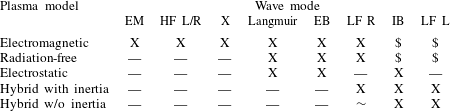
Table 7 at the end lists which wave modes are suitable for each plasma model, allowing for a quick selection of the relevant description following below.
3.1 Electromagnetic mode
The first wave we want to consider is the electromagnetic wave. It also exists as a solution to Maxwell’s equations in vacuum, where it has the trivial dispersion relation
 $$\begin{eqnarray}\unicode[STIX]{x1D714}=ck.\end{eqnarray}$$
To obtain the equivalent dispersion relation in a plasma, let us first consider the
case without a background magnetic field. In that case,
 $D$
vanishes and
 $P=R=L=S=1-\unicode[STIX]{x1D714}_{p}^{2}/\unicode[STIX]{x1D714}^{2}$
, with the joint plasma frequency
 $\unicode[STIX]{x1D714}_{p}$
of all species given by:
 $$\begin{eqnarray}\unicode[STIX]{x1D714}_{p}=\sqrt{\mathop{\sum }_{\unicode[STIX]{x1D6FC}}\unicode[STIX]{x1D714}_{p,\unicode[STIX]{x1D6FC}}^{2}}.\end{eqnarray}$$
This simplifies the Maxwell tensor significantly and the resulting characteristic polynomial can be solved, yielding the following dispersion relation for the electromagnetic wave:
 $$\begin{eqnarray}\unicode[STIX]{x1D714}^{2}=\unicode[STIX]{x1D714}_{p}^{2}+c^{2}k^{2}.\end{eqnarray}$$
Equation (3.18) indicates that this
wave has a low-frequency cutoff at the plasma frequency
 $\unicode[STIX]{x1D714}_{p}$
and extends to arbitrarily large frequencies. In numerical
practice, there is a high-frequency limit from the Nyquist frequency that the grid
imposes on the wavelength. The high-frequency nature makes the electromagnetic mode
very suitable for a quick check of a simulation code implementing the electromagnetic
plasma model, as relatively few time steps are needed.
3.2 Magnetic birefringence
The addition of a background magnetic field splits the electromagnetic mode into two
modes. For parallel propagation (
 $\unicode[STIX]{x1D717}=0$
) these are the
 $L$
and
 $R$
mode. Their respective dispersion relations are:
 $$\begin{eqnarray}n^{2}=L,\quad n^{2}=R.\end{eqnarray}$$
The
 $L$
mode is left-hand circularly polarized while the
 $R$
mode right handed. This motivates their name and the name of the
corresponding Stix parameter. Solving for
 $\unicode[STIX]{x1D714}(k)$
is possible, but leads to rather long expressions. Both modes
behave very much like the electromagnetic mode but with a shifted cutoff. Their
cutoff frequencies are given by
 $$\begin{eqnarray}\displaystyle & \displaystyle \unicode[STIX]{x1D714}_{cut,L}={\textstyle \frac{1}{2}}\left((\unicode[STIX]{x1D6FA}_{c,i}-\unicode[STIX]{x1D6FA}_{c,e})+\sqrt{(\unicode[STIX]{x1D6FA}_{c,e}+\unicode[STIX]{x1D6FA}_{c,i})^{2}+4\unicode[STIX]{x1D714}_{p}^{2}}\right), & \displaystyle\end{eqnarray}$$
 $$\begin{eqnarray}\displaystyle & \displaystyle \unicode[STIX]{x1D714}_{cut,R}={\textstyle \frac{1}{2}}\left((\unicode[STIX]{x1D6FA}_{c,e}-\unicode[STIX]{x1D6FA}_{c,i})+\sqrt{(\unicode[STIX]{x1D6FA}_{c,e}+\unicode[STIX]{x1D6FA}_{c,i})^{2}+4\unicode[STIX]{x1D714}_{p}^{2}}\right). & \displaystyle\end{eqnarray}$$
In the limit of
 $\unicode[STIX]{x1D714}_{cut}\gg \unicode[STIX]{x1D6FA}_{c,e}\gg \unicode[STIX]{x1D6FA}_{c,i}$
, the right-hand sides of (3.20) and (3.21) simplify
to
 $\unicode[STIX]{x1D714}_{p}\pm 1/2\unicode[STIX]{x1D6FA}_{c,e}$
. The
 $L$
and
 $R$
modes have a second branch at much lower frequencies, below the
gyro-frequencies of ions and electrons respectively. These exist even in
radiation-free plasma models and provide a suitable test problem for them.
In this range of frequencies, that is especially relevant for EMHD or hybrid simulations, the dispersion relation of the right-hand circular mode can be found in e.g. Bulanov, Pegoraro & Sakharov (Reference Bulanov, Pegoraro and Sakharov1992) or Shaikh (Reference Shaikh2009) and is given by:
 $$\begin{eqnarray}\unicode[STIX]{x1D714}=\unicode[STIX]{x1D6FA}_{c,e}\frac{d_{e}^{2}k^{2}}{1+d_{e}^{2}k^{2}}.\end{eqnarray}$$
The product of electron skin depth
 $d_{e}$
and the wavenumber
 $k$
can be expected to be not too large. In the limit
 $kd_{e}\gg 1$
the wave frequency has the limiting value
 $\unicode[STIX]{x1D714}\rightarrow \unicode[STIX]{x1D6FA}_{c,e}$
, however the wave is usually absorbed before that.
In a hybrid model without electron inertia the nature of the low-frequency
 $R$
mode changes. To derive the dispersion relation, it is necessary to
insert the definitions of gyro-frequency
 $\unicode[STIX]{x1D6FA}_{c,e}$
and electron skin depth
 $d_{e}$
into (3.22) and
take the limit
 $m_{e}\rightarrow 0$
. Doing so leads to
 $$\begin{eqnarray}\unicode[STIX]{x1D714}=\frac{cB}{4\unicode[STIX]{x03C0}n_{e}e}k^{2},\end{eqnarray}$$
which is well defined even in the absence of electron inertia.
However, at larger
 $k$
it lacks the cutoff at the electron gyro-frequency, which is not
well defined without electron mass.
3.3 Extraordinary mode
In the case of perpendicular propagation (i.e.
 $\unicode[STIX]{x1D717}=\unicode[STIX]{x03C0}/2$
), we also find that the electromagnetic mode is split into a pair
of modes. The mode where the electric field component is parallel to the background
magnetic field behaves just as in the unmagnetized case. This is called the ordinary
mode (or in short
 $O$
mode). The other mode, which only exists in the presence of a
static magnetic field, is called extraordinary mode (or
 $X$
mode). Its electric field component is perpendicular to both
 $k$
and
 $B_{0}$
. The dispersion relation of this second mode is given by
 $$\begin{eqnarray}\frac{c^{2}k^{2}}{\unicode[STIX]{x1D714}^{2}}=\frac{((\unicode[STIX]{x1D714}+\unicode[STIX]{x1D6FA}_{c,i})(\unicode[STIX]{x1D714}-\unicode[STIX]{x1D6FA}_{c,e})-\unicode[STIX]{x1D714}_{p}^{2})((\unicode[STIX]{x1D714}-\unicode[STIX]{x1D6FA}_{c,i})(\unicode[STIX]{x1D714}+\unicode[STIX]{x1D6FA}_{c,e})-\unicode[STIX]{x1D714}_{p}^{2})}{(\unicode[STIX]{x1D714}^{2}-\unicode[STIX]{x1D6FA}_{c,i}^{2})(\unicode[STIX]{x1D714}^{2}-\unicode[STIX]{x1D6FA}_{c,e}^{2})+\unicode[STIX]{x1D714}_{p}^{2}(\unicode[STIX]{x1D6FA}_{c,e}\unicode[STIX]{x1D6FA}_{c,i}-\unicode[STIX]{x1D714}^{2})}.\end{eqnarray}$$
This mode has a cutoff at
 $$\begin{eqnarray}\unicode[STIX]{x1D714}_{cut,X}=\unicode[STIX]{x1D714}_{cut,R}={\textstyle \frac{1}{2}}\left(\unicode[STIX]{x1D6FA}_{c,e}-\unicode[STIX]{x1D6FA}_{c,i}+\sqrt{(\unicode[STIX]{x1D6FA}_{c,e}+\unicode[STIX]{x1D6FA}_{c,i})^{2}+4\unicode[STIX]{x1D714}_{p}^{2}}\right).\end{eqnarray}$$
This frequency is close to the upper hybrid frequency which is given by
 $$\begin{eqnarray}\unicode[STIX]{x1D714}_{UH}\approx \sqrt{\unicode[STIX]{x1D6FA}_{c,e}^{2}+\unicode[STIX]{x1D714}_{p}^{2}}.\end{eqnarray}$$
Depending on the magnetization, a second branch of the extraordinary mode close the plasma frequency exists. If it exists it has a lower cutoff frequency
 $$\begin{eqnarray}\unicode[STIX]{x1D714}_{cut,X}^{\prime }=\unicode[STIX]{x1D714}_{cut,L}={\textstyle \frac{1}{2}}\left(\unicode[STIX]{x1D6FA}_{c,i}-\unicode[STIX]{x1D6FA}_{c,e}+\sqrt{(\unicode[STIX]{x1D6FA}_{c,e}+\unicode[STIX]{x1D6FA}_{c,i})^{2}+4\unicode[STIX]{x1D714}_{p}^{2}}\right).\end{eqnarray}$$
3.4 Langmuir mode
If we return to the case without a magnetic background field and re-examine the
dielectric tensor as given in (3.15), we notice that the characteristic polynomial has three solutions. Two
of them are identical and belong to the electromagnetic mode – discussed above – with
two independent degrees of freedom (either two linearly polarized modes or
equivalently two circularly polarized modes). However, there exists a third solution
to
 $|\unicode[STIX]{x1D63F}(\unicode[STIX]{x1D714},\boldsymbol{k})|=0$
which satisfies
 $\unicode[STIX]{x1D714}=\unicode[STIX]{x1D714}_{p}$
. This describes plasma oscillations which – for a cold plasma –
have constant frequency, vanishing group velocity and are purely electrostatic.
To obtain a wave mode with well-defined propagation behaviour and wavenumber
dependence, it is necessary to include the effects of a finite temperature in a warm
plasma. This can be done for any wave mode but is tedious as the permittivity tensor
needs to be redefined to include the distribution function. In the case of a
Maxwellian velocity distribution, this is generally expressed using the plasma
dispersion function
 $Z(\unicode[STIX]{x1D701})$
(see Fried & Conte Reference Fried and Conte1961). Solving the resulting equations to get the dispersion relations is
complicated by the extra terms or might even be impossible to do analytically in the
general case. For the test problems, it is sufficient to proceed in a less rigorous
manner with the Langmuir mode. Assuming an electron temperature
 $T_{e}$
, we can modify the dielectric permittivity tensor to include the
leading term, resulting in:
 $$\begin{eqnarray}\unicode[STIX]{x1D716}=1-\frac{\unicode[STIX]{x1D714}_{p}^{2}}{\unicode[STIX]{x1D714}^{2}}-3\frac{k^{2}\unicode[STIX]{x1D714}_{p}^{2}}{m_{e}\unicode[STIX]{x1D714}^{4}}T_{e}.\end{eqnarray}$$
Solving for
 $\unicode[STIX]{x1D714}^{2}$
to get the dispersion relation, we end up with
 $$\begin{eqnarray}\unicode[STIX]{x1D714}^{2}=\frac{1}{2}\left(\unicode[STIX]{x1D714}_{p}^{2}+\sqrt{\unicode[STIX]{x1D714}_{p}^{4}+12\frac{k^{2}T_{e}}{m_{e}\unicode[STIX]{x1D714}_{p}^{2}}}\right),\end{eqnarray}$$
which of course for infinitely small
 $k$
is just
 $\unicode[STIX]{x1D714}_{p}^{2}$
and can be approximated, for not too large
 $k$
, by
 $$\begin{eqnarray}\unicode[STIX]{x1D714}^{2}=\unicode[STIX]{x1D714}_{p}^{2}+3k^{2}T_{e}/m_{e}.\end{eqnarray}$$
At this point, it is useful to introduce the Debye length
 $\unicode[STIX]{x1D706}_{D}$
. This is the natural length scale below which the plasma might
contain charge imbalances and electrostatic fields. The (electron) Debye length is
given by
 $$\begin{eqnarray}\unicode[STIX]{x1D706}_{D}=\sqrt{\frac{T_{e}}{m_{e}\unicode[STIX]{x1D714}_{p}^{2}}}=\frac{v_{th,e}}{\unicode[STIX]{x1D714}_{p}}.\end{eqnarray}$$
We can rewrite the dispersion relation of the Langmuir mode as
 $$\begin{eqnarray}\unicode[STIX]{x1D714}^{2}=\unicode[STIX]{x1D714}_{p}^{2}\cdot (1+3k^{2}\unicode[STIX]{x1D706}_{D}^{2}).\end{eqnarray}$$
The second term in this formulation being the correction due to the finite
temperature and Debye length. This expression is reasonably accurate as long as the
second term is less than unity, which fortunately is the case as Langmuir waves of
higher
 $k$
are quickly damped by electron Landau damping (see Dawson Reference Dawson1961). This is a completely collisionless effect
resulting from the interaction of the Langmuir wave with kinetic electrons and as
such is not applicable when electrons are described as a fluid.
3.5 Bernstein modes
For the final wave mode considered in this set of test problems, we again add a
background magnetic field and look at the longitudinal modes that propagate
perpendicular to the background field. These waves also exist only in a plasma of
finite temperature, because only there is the gyro-radius finite. For a particle of
species
 $\unicode[STIX]{x1D6FC}$
the gyro-radius
 $r_{\unicode[STIX]{x1D6FC}}$
is given by:
 $$\begin{eqnarray}r_{\unicode[STIX]{x1D6FC}}=\sqrt{\frac{k_{B}T_{\unicode[STIX]{x1D6FC}}}{m_{\unicode[STIX]{x1D6FC}}\unicode[STIX]{x1D6FA}_{c,\unicode[STIX]{x1D6FC}}^{2}}}=\frac{v_{th,\unicode[STIX]{x1D6FC}}}{\unicode[STIX]{x1D6FA}_{c,\unicode[STIX]{x1D6FC}}}.\end{eqnarray}$$
The original derivation of the dispersion relation can be found in Bernstein (Reference Bernstein1958) and will not be repeated here. To write the dispersion relation it is useful to rescale the wavenumber using the gyro-radius as follows:
 $$\begin{eqnarray}\unicode[STIX]{x1D706}_{\unicode[STIX]{x1D6FC}}=k^{2}r_{\unicode[STIX]{x1D6FC}}^{2}.\end{eqnarray}$$
This quantity is non-zero in a warm plasma, corresponding to the presence of finite
Larmor radius effects. If
 $\unicode[STIX]{x1D706}_{\unicode[STIX]{x1D6FC}}$
is small this mostly leads to gyro-resonances at integer multiples
of the gyro-frequencies. The situation becomes complicated if we cannot make this
assumption. At least for the case of electrostatic waves propagating exactly
perpendicular to the background magnetic field, we can find the dispersion relation
e.g. in Swanson (Reference Swanson2003). Using the different
definition of thermal speed implicitly used in (3.33) and rewriting in terms of quantities defined in this
paper, we find:
 $$\begin{eqnarray}1-\mathop{\sum }_{\unicode[STIX]{x1D6FC}}\frac{2\unicode[STIX]{x1D714}_{p,\unicode[STIX]{x1D6FC}}^{2}}{\unicode[STIX]{x1D706}_{\unicode[STIX]{x1D6FC}}}\text{e}^{-\unicode[STIX]{x1D706}_{\unicode[STIX]{x1D6FC}}}\mathop{\sum }_{n=1}^{\infty }\frac{n^{2}\text{I}_{n}(\unicode[STIX]{x1D706}_{\unicode[STIX]{x1D6FC}})}{\unicode[STIX]{x1D714}^{2}-n^{2}\unicode[STIX]{x1D6FA}_{c,\unicode[STIX]{x1D6FC}}^{2}}=0.\end{eqnarray}$$
This expression uses modified Bessel functions
 $\text{I}_{n}$
of the first kind. For frequencies of the order of the electron
gyro-frequency and higher, the ions can be considered stationary and all terms
connected to them can be dropped. This removes the splitting of each mode into a
group of related modes separated by multiples of the ion gyro-frequency as this is
hard to resolve experimentally and numerically and is neglected here. The dispersion
relation then simplifies and reads:
 $$\begin{eqnarray}1-\frac{2\unicode[STIX]{x1D6FA}_{c,e}^{2}}{k^{2}\unicode[STIX]{x1D706}_{D}^{2}}\text{e}^{-\unicode[STIX]{x1D706}_{e}}\mathop{\sum }_{n=1}^{\infty }\frac{n^{2}\text{I}_{n}(\unicode[STIX]{x1D706}_{e})}{\unicode[STIX]{x1D714}^{2}-n^{2}\unicode[STIX]{x1D6FA}_{c,e}^{2}}=0.\end{eqnarray}$$
It is also possible to consider Bernstein waves at lower frequencies. At ion length
scales of
 $\unicode[STIX]{x1D706}_{i}\approx 1$
we find that
 $\unicode[STIX]{x1D706}_{e}\approx m_{e}/m_{i}\unicode[STIX]{x1D706}_{i}\ll 1$
. Given that the Bessel function of order
 $n>1$
vanishes for small arguments, this implies that we can drop the
electron terms when considering ion scales. In this limit (3.35) can be approximated by:
 $$\begin{eqnarray}1-\frac{\unicode[STIX]{x1D714}_{p,e}^{2}}{\unicode[STIX]{x1D6FA}_{c,e}^{2}}-\frac{2\unicode[STIX]{x1D6FA}_{c,i}^{2}}{k^{2}\unicode[STIX]{x1D706}_{D}^{2}}\text{e}^{-\unicode[STIX]{x1D706}_{i}}\mathop{\sum }_{n=1}^{\infty }\frac{n^{2}\text{I}_{n}(\unicode[STIX]{x1D706}_{i})}{\unicode[STIX]{x1D714}^{2}-n^{2}\unicode[STIX]{x1D6FA}_{c,i}^{2}}=0.\end{eqnarray}$$
The term containing electron quantities is not present in the same way for electron Bernstein waves and represents a shielding effect from the electrons.
For high orders of
 $n$
the simplification of representing the electrons by a constant term
becomes increasingly wrong, especially if the mass ratio
 $m_{i}/m_{e}$
is not sufficiently large. However, as can be seen from the
parameters in table 5, this is not a problem
for the test case presented here.
4 Numerical implementation
Most of the simulations that were performed to produce the illustrations in this paper used the PIC Code ACRONYM (Kilian, Burkart & Spanier Reference Kilian, Burkart, Spanier, Nagel, Krner and Resch2012) or extensions thereof. This simulation code is quite flexible and implements a wide range of plasma models. The simulation domain can be simulated with one, two or three spatially resolved dimensions (fields and velocities are always represented by three component vectors) and their boundaries can be periodic, reflecting or absorbing. For the test case, only one spatially resolved dimension and periodic boundary conditions are used to reduce numerical effort and implementation requirements.
Kinetic species are represented by macroparticles. Their charge and current density is
deposited onto the grid using second-order interpolation with the triangular-shaped
cloud (TSC) shape function. The current is deposited based on the same shape function
using
 $q\boldsymbol{v}$
for one-dimensional simulations or with the charge-conserving method
of Esirkepov (Reference Esirkepov2001) for two- and
three-dimensional simulations.
Electrons in the plasma can be represented either in this way for fully kinetic simulations, or implicitly as a fluid with or without electron inertia, following the EMHD solver of Jain et al. (Reference Jain, Das, Kaw and Sengupta2003).
4.1 Electromagnetic
In electromagnetic simulations, the electric and magnetic fields are evolved from the homogeneous initial state using the finite-difference time domain (FDTD) method:
 $$\begin{eqnarray}\left.\begin{array}{@{}c@{}}\boldsymbol{B}^{t+1/2}=\boldsymbol{B}^{t-1/2}-c\unicode[STIX]{x0394}t\unicode[STIX]{x1D735}\times \boldsymbol{E}^{t},\\ \boldsymbol{E}^{t+1}=\boldsymbol{E}^{t}+c\unicode[STIX]{x0394}t\unicode[STIX]{x1D735}\times \boldsymbol{B}^{t+1/2}-4\unicode[STIX]{x03C0}\unicode[STIX]{x0394}t\boldsymbol{j}^{t+1/2}.\end{array}\right\}\end{eqnarray}$$
The field quantities are stored in a staggered grid following the idea by Yee (Reference Yee1966), which allows for a very straightforward
calculation of the curl that is accurate to second order. This field solver leads to
a modification of the dispersion relation at large
 $\unicode[STIX]{x1D714}$
and
 $k$
. In the case of the electromagnetic mode propagating along one axis
of the spatial grid, the resulting dispersion relation is
 $$\begin{eqnarray}\left(\frac{2}{\unicode[STIX]{x0394}t}\right)^{2}\sin ^{2}\left(\frac{\unicode[STIX]{x1D714}\unicode[STIX]{x0394}t}{2}\right)=\unicode[STIX]{x1D714}_{p}^{2}+c^{2}\left(\frac{2}{\unicode[STIX]{x0394}x}\right)^{2}\sin ^{2}\left(\frac{k\unicode[STIX]{x0394}x}{2}\right).\end{eqnarray}$$
For frequencies that are not close to the respective Nyquist limit, the modification is negligible.
4.2 Radiation free
The numerical implementation of the radiation-free model is harder than (2.9)–(2.11) imply at first. The reason is the fact that
 $\boldsymbol{E}_{T}$
depends on the time derivative of the transverse component
 $\boldsymbol{j}_{T}$
of the current. The change in current, however, is of course
connected to the acceleration of the particles which in turn depends on the electric
field. An overly naive time discretization is therefore violently unstable. Our code
follows the method of Decyk (Reference Decyk2011), which
solves the problem in the following way.
In the first part of a time step, the charge density
 $\unicode[STIX]{x1D70C}$
is deposited onto the grid and (2.11) is solved with a Fourier-based solver to get
 $\boldsymbol{E}_{L}$
.
The new values of
 $\boldsymbol{E}_{T}$
and
 $\boldsymbol{B}$
are calculated using the following iterative scheme: first
 $\boldsymbol{j}$
and
 $\unicode[STIX]{x2202}\boldsymbol{j}/\unicode[STIX]{x2202}t$
are deposited onto the grid using the assumption that the particle
velocities remain unchanged.
Once the current contributions are known, it is possible to solve for the field components. And as soon as all fields are known, a better prediction of the particle velocities can be made. Using the better estimate for the particle velocities, a better estimate of the current can be deposited onto the grid. This, in turn, allows for a refinement of the field components.
The iteration scheme converges quickly, after two or three iterations. At this point, the particle velocity can be updated based on the best current prediction for the new velocity and the code can proceed to the next time step.
4.3 Electrostatic
The electrostatic model uses a spectral solver to calculate the longitudinal electric field. This solver makes use of the fact that the charge density can be replaced by its Fourier series
 $$\begin{eqnarray}\unicode[STIX]{x1D70C}(\boldsymbol{r})=\mathop{\sum }_{kx,ky,kz}\tilde{\unicode[STIX]{x1D70C}}(\boldsymbol{k})\exp (\text{i}k_{x}x+\text{i}k_{y}x+\text{i}k_{z}z)\end{eqnarray}$$
in (2.11). The components of the electric field can be rewritten in the same way and the derivative can act directly on the exponential functions. As the different Fourier modes are orthogonal, the resulting equation has to be satisfied for each mode separately, which leads to the following relation between the charge density and the electric field in the spectral domain:
 $$\begin{eqnarray}\tilde{\boldsymbol{E}}(\boldsymbol{k})=-4\unicode[STIX]{x03C0}\text{i}\frac{\tilde{\unicode[STIX]{x1D70C}}(\boldsymbol{k})\boldsymbol{k}}{|\boldsymbol{k}|^{2}}.\end{eqnarray}$$
This way, the electric field can be calculated by performing a Fourier transform on
 $\unicode[STIX]{x1D70C}$
, multiplying every component in
 $k$
-space with
 $-4\unicode[STIX]{x03C0}\text{i}\boldsymbol{k}|\boldsymbol{k}|^{-2}$
, which can be considered a convolution with the Green function of
free space and transforming the resulting field back to real space.
Both the radiation-free model and the electrostatic model have a gap at
 $k=0$
in the spectrum of the electric field. This is an artefact of
solving Poisson’s equation in the Fourier domain. The only possible source term that
would produce
 $\tilde{E}(k=0)$
is
 $\tilde{\unicode[STIX]{x1D70C}}(k=0)$
. This quantity, however, is the net charge density which vanishes
when averaging over the entire simulation domain that contains an equal number of
positive and negative charged particles.
4.4 Vlasov-hybrid simulation
We also used a second independent implementation of the electrostatic plasma models, which is not based on the PIC method, but instead follows the Vlasov-hybrid simulation (VHS) method by Nunn (Reference Nunn1993). This method is not a hybrid between a kinetic and a fluid part as described in the following subsection, but a hybrid between an Eulerian description of phase space density and a Lagrangian description using macroparticles. Whereas a PIC code represents chunks of phase space density as macroparticles of constant weight and deposits their charge or current onto a grid, a VHS code reconstructs the phase space density on a grid. It then integrates out the velocity direction(s) to obtain moments of the distribution function such as charge density. The reconstruction step requires extra effort but allows for the use of macroparticles with significantly different weights without losing the effect of markers that represent low phase space density. This makes VHS a technique with a very low level of numerical noise. An open source implementation and a description of the code have been submitted for publication elsewhere.
4.5 Implicit electron fluid
Details of the hybrid code are described in Muñoz et al. (Reference Muñoz, Jain, Kilian and Büchner2016). On a high level it computes the time
evolution of the ions, just as a PIC code would, and determines the ions charge
density
 $n_{i}$
and current density
 $\boldsymbol{j}_{i}$
. Using those the generalized vorticity can be updated as described
in (2.13). After that, the magnetic
field
 $\boldsymbol{B}$
can be computed from a version of (2.14), where the electron flow speed has been eliminated using
(2.15). Then the electric field
 $\boldsymbol{E}$
can be determined from the generalized Ohm’s law given in (2.12).
4.6 Linearized dielectric tensor
To verify the analytically known plasma modes and to check for thermal effects that are neglected in their cold plasma description, we also used the ‘Waves in homogeneous, anisotropic, multicomponent plasmas’ (WHAMP) code (see Roennmark Reference Roennmark1982). This code does not evolve the full plasma model but starts with the linearization of the time-independent equations. Assuming a parametrized velocity distribution function it uses analytic expressions to approximate the dielectric tensor of a warm multicomponent plasma. The plasma dispersion function that is needed in that description is numerically approximated by a Padé approximation and the resulting tensor is solved numerically using Newton iteration.
For a given wavenumber
 $k$
WHAMP not only provides the real part of the wave frequency, but
also the growth or damping rate given by the imaginary part of
 $\unicode[STIX]{x1D714}$
. This could be used to study waves that are driven by some source
of free energy. As long as the wave amplitude is sufficiently small, it is possible
to measure growth rate in a way similar to Schreiner, Kilian & Spanier (Reference Schreiner, Kilian and Spanier2016) and compare to analytic predictions, if
available, or the results from WHAMP. This is however beyond the scope of the test
problems in this paper.
5 Test problems
It is not easy to choose plasma parameters that are accessible to a large range of
simulation codes and that produce results that can be compared in a meaningful manner.
This can be seen, for example, in the case of the thermal speed of electrons. Very small
values – and consequently low temperatures – make the comparison with predictions for
cool or cold plasmas easier. Explicit PIC codes, on the other hand, have small time
steps that are set by the speed of light. If thermal particles move at a tiny fraction
of the speed of light, they only move a tiny distance per time step and the code has to
compute many time steps. As a compromise and to avoid relativistic effects, an electron
thermal speed of 5 % of the speed of light was chosen. All three initial velocity
components of the electrons are drawn independently from a normal distribution with zero
mean and standard deviation
 $v_{th,e}$
. Using the relation
 $m_{e}v_{th,e}^{2}=k_{B}T_{e}$
, we determine the equivalent temperature of 14.79 MK.
The plasma contains protons (single positive charge, natural mass ratio unless
specifically noted otherwise) as neutralizing (ion) species. The ion temperature
 $T_{i}$
is set equal to the electron temperature, therefore, their thermal
speed is lower by a factor of
 $\sqrt{m_{i}/m_{e}}$
.
The absolute value of the plasma frequency has no such direct physical implications.
However, it sets the Debye length and thereby the size of the grid cells. A value of
 $10^{9}~\text{rad}~\text{s}^{-1}$
was chosen for the electrons, which corresponds to a density of
 $3.14\times 10^{8}$
particles per cubic centimetre. The protons have the same density to
fulfil charge neutrality, which translates to a proton plasma frequency of
 $2.33\times 10^{7}~\text{rad}~\text{s}^{-1}$
. The contribution of the protons to the total plasma frequency is
negligible.
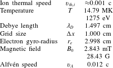
Using these temperature and frequency scales, the Debye length turns out to be 1.497 cm. To avoid grid heating and other numerical effects, the cell size of each grid cell should be slightly smaller (see e.g. Birdsall & Langdon Reference Birdsall and Langdon2005), which suggests the round value of 1 cm.
The only physical parameter that still needs to be specified is the magnetic field
strength. Here we select 2.843 mT which corresponds to a high density plasma with
 $2\unicode[STIX]{x1D6FA}_{c,e}=\unicode[STIX]{x1D714}_{p,e}$
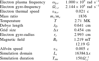
. Table 1 lists all the
defining parameters in compact form and table 2
has some other derived plasma parameters.
Common choice of simulation parameters to be used in all simulations unless noted otherwise.

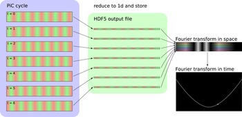
Sketch of the analysis pipeline.

Resulting plasma parameters based on the choices made in table 1.

Some of the simulations that depend on one spatial dimension were actually run with a three-dimensional PIC code with a width of 4 cells and periodic boundary conditions in the negligible directions. Each cell contains eight computational macroparticles per species.
After the numerical simulation has been performed, it is necessary to extract properties
of the wave modes and compare with the expected behaviour. To this end it is very useful
to plot the energy density of a field component as a function of
 $k$
and
 $\unicode[STIX]{x1D714}$
. The energy density is sharply localized along linear wave modes and
characteristic frequencies (e.g. the low-frequency cutoff of the electromagnetic mode)
can easily and reliably be extracted.
Figure 1 shows a sketch of the analysis that is
performed. For the following explanation, we assume that we are interested in one
component of the transverse electric field, other field components work analogously.
Depending on the simulation code,
 $E_{x}(z,t)$
or possibly
 $E_{x}(x,y,z,t)$
is computed at every time step. This quantity is stored along with the
necessary meta-data in a file using the 5th version of the Hierarchical Data Format
(HDF5) for later analysis.
As I/O can be a bottleneck for the simulation code, it is desirable to reduce overall
output requirements. For the study of low-frequency wave modes, it is usually sufficient
to perform output every
 $N_{io}$
time steps as long as
 $$\begin{eqnarray}\frac{\unicode[STIX]{x03C0}}{N_{io}\unicode[STIX]{x0394}t}=\frac{\unicode[STIX]{x03C0}}{\unicode[STIX]{x0394}t_{io}}<\unicode[STIX]{x1D714}\end{eqnarray}$$
holds for the highest frequency
 $\unicode[STIX]{x1D714}$
that is of interest. Similarly, it should be considered whether the
code can average over the negligible directions before performing output.
In post-processing,
 $E_{x}(z,t)$
is Fourier transformed in space and time to yield
 $\tilde{E}_{x}(k_{z},\unicode[STIX]{x1D714})$
. To scale the axis correctly, it is useful to know that the frequency
range one gets out of snapshots that are separated by
 $\unicode[STIX]{x0394}t_{io}$
is
 $0\ldots \unicode[STIX]{x03C0}/t_{io}$
in steps of
 $\unicode[STIX]{x03C0}/T_{sim}$
. The range in
 $k$
is
 $-\unicode[STIX]{x03C0}/\unicode[STIX]{x0394}x\ldots \unicode[STIX]{x03C0}\unicode[STIX]{x0394}x$
. In most cases it is advisable to rescale from the units used in the
code – Gaussian cgs with values in in 1/s and 1/cm for the codes used here – to plasma
scales such as
 $\unicode[STIX]{x1D714}_{p}$
or
 $\unicode[STIX]{x1D6FA}_{c,e}$
before plotting.
5.1 Test 1: electromagnetic mode
The cheapest test is designed to capture the electromagnetic mode. It does not use any background magnetic field and the size is given in table 3.
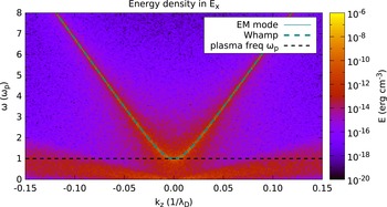
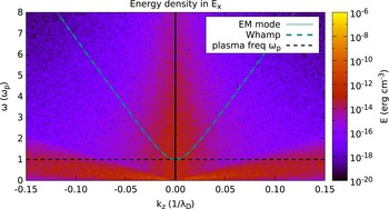
Energy density in one transverse component of the electric field as
simulated by the electromagnetic plasma model. The electromagnetic mode is
clearly visible, including the cutoff at the plasma frequency
 $\unicode[STIX]{x1D714}_{p}$
. The simulation parameters can be found in tables 3 and 1, but the simulation is performed without a magnetic
field.

Simulation size to study the electromagnetic mode.

Figure 2 shows that the energy is mostly
concentrated along the dispersion relation predicted by cold plasma theory (given by
(3.18), shown as a dashed line)
and has a cutoff at the plasma frequency
 $\unicode[STIX]{x1D714}_{p}$
, which is indicated by the horizontal dashed line. Predictions for
the absolute magnitude and the low-frequency noise are given in Sitenko (Reference Sitenko1967), but are not discussed here.
This mode is the cheapest way to determine the plasma frequency from the simulated data and to compare it to the desired value from the simulation input. Many numerical problems (wrong normalization, errors in the charge or current deposition, problems in the particle pusher) can alter this mode, so it is ideally suited as a quick regression check after code modifications.
At large
 $k$
– closer to the Nyquist limit imposed by the grid size
 $\unicode[STIX]{x0394}x$
– numerical dispersion effects occur that result from the discrete
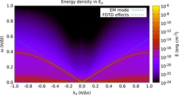
Maxwell solver in the simulation code. Figure 3
shows this effect of the FDTD algorithm that is used to solve Maxwell’s equations in
time. The modified dispersion relation is given by (4.2), in good agreement with our results.
Spectral energy density up to the resolution limits permitted by the finite
cell size and time step length. This plot uses data from the same simulation
as figure 2. At high frequencies and
large
 $k$
close to
 $\pm \unicode[STIX]{x03C0}/\unicode[STIX]{x0394}x$
, significant numerical dispersion is visible.


In the radiation-free plasma model, the electromagnetic mode is explicitly removed.
The remaining part of the transverse spectrum is shown in figure 4. No well-defined mode is left in the unmagnetized case. At small
 $\unicode[STIX]{x1D714}$
and low phase velocities, a diffuse mode is visible that can be
identified as ion acoustic waves. These, however, have a broadband spectrum without
sharp features that would provide a good test problem.
The increase in noise at low
 $k$
can be attributed to a well known numerical instability at scales
larger than the electron skin depth in the radiation-free plasma model. This
instability can be removed through the introduction of a shift constant in the
equation for the transverse electric field, but some noise remains (see Decyk Reference Decyk2011, for details).
5.2 Test 2: high-frequency
 $L$
and
$R$
modes


The addition of a background magnetic field (of 2.843 mT in this test problem) along
the
 $z$
direction splits the electromagnetic mode into two modes with
circular polarization.
To study polarization properties of the waves, one switches from a standard Cartesian
basis (with transverse components
 $\hat{x},{\hat{y}}$
) to a circular basis. In plasma physics phase convention, the new
basis vectors are given by
 $$\begin{eqnarray}\displaystyle & \displaystyle \hat{l}=\frac{1}{\sqrt{2}}(\hat{x}-\text{i}{\hat{y}}), & \displaystyle\end{eqnarray}$$
 $$\begin{eqnarray}\displaystyle & \displaystyle \hat{r}=\frac{1}{\sqrt{2}}(\hat{x}+\text{i}{\hat{y}}). & \displaystyle\end{eqnarray}$$
Instead of performing the analysis that is sketched in figure 1 on a field component in the Cartesian basis (e.g.
 $E_{x}(z,t)$
), it is possible to combine
 $E_{x}(z,t)$
and
 $E_{y}(z,t)$
in the following way:
 $$\begin{eqnarray}E_{l,r}=\frac{1}{\sqrt{2}}(E_{x}(z,t)\mp \text{i}E_{y}(z,t)).\end{eqnarray}$$
As usual, a Fourier transform in space and time is performed to yield
 $\tilde{E}_{l,r}(k_{z},\unicode[STIX]{x1D714})$
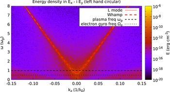
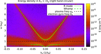
. Figures 5 and 6 show the spectral energy density
 $|\tilde{E}_{l,r}|^{2}$
respectively.
Energy density in the left-handed circularly polarized component of the
electric field produced by the electromagnetic plasma model. This plot is
based on parameters given in tables 3 and 1. The spectral
energy density is concentrated along the high-frequency branch of the
 $L$
mode, propagating along the background magnetic field.

Energy density in the right-handed circularly polarized component of the
electric field produced by the electromagnetic plasma model. This plot uses
the same parameters as figure 5, but
the simulation results are combined differently to display the other
circular polarization basis. Both high- and low-frequency branches of the
 $R$
mode are visible.

In the circular basis only the wave modes with the matching circular polarization
appear, thus confirming that the numerical implementation reproduces the expected
polarization properties. Both modes follow the analytically predicted dispersion
relation given in (3.19a,b
). The cutoff is shifted (away from the cutoff at
 $\unicode[STIX]{x1D714}_{p}$
in the unmagnetized case) by about
 $\pm 1/2\,\unicode[STIX]{x1D6FA}_{c,e}$
as expected.
In the right-hand polarization, shown in figure 6, two additional features are visible. One is a low-frequency component
with a resonance at
 $\unicode[STIX]{x1D6FA}_{c,e}$
, which will be studied in more detail in a following test. The
other feature is a triangular region of fluctuations that is caused by gyrating
electrons. Within that region that is centred on
 $\unicode[STIX]{x1D6FA}_{c,e}$
and bounded by approximately
 $\pm 3\,v_{th,e}\,k$
, the dispersion relation of the
 $R$
mode is modified. At larger
 $k$
the wave is absorbed. Both effects are captured by WHAMP and
studied in more detail in Test 6.
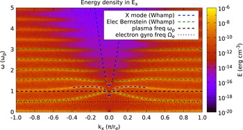
5.3 Test 3: extraordinary mode
Keeping the background magnetic field along
 $z$
and rotating the simulation box to point along
 $x$
, allows to study waves that propagate across the magnetic field.
(Alternatively, one can change the direction of the magnetic field, in which case
field components switch behaviour.)
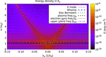
As expected, the field component perpendicular to
 $k$
and
 $B_{0}$
shows the extraordinary mode. Both the high-frequency branch above
the upper hybrid frequency and the branch close to the plasma frequency show the
expected dispersion relation given in (3.24). Thermal effects are not important for this mode, as can be seen by
the excellent agreement between the predictions of cold plasma theory and the
numerical solution by WHAMP that includes finite temperature effects.
Figure 7 also shows approximately horizontal features at harmonics of the electron gyro-frequency. These are due to electron Bernstein waves which can only be explained by the thermal effects and are studied in more detail in Test 7.
Energy density in the electric field component that is perpendicular to both the background magnetic field and the propagation direction. The plot shows simulation results from the electromagnetic plasma model with parameters given in tables 3 and 1. Both branches of the X mode are clearly visible. Due to the finite temperature, harmonics of the electron gyro-frequency and the first few electron Bernstein modes are also visible.

5.4 Test 4: Langmuir mode
This test problem focuses on longitudinal waves which, in the unmagnetized case, are
represented by the Langmuir mode. As mentioned previously, this mode is a result of
plasma oscillations in a plasma of finite temperature. Consequently, it can be used
to determine the thermal speed of the electrons
 $v_{th,e}$
and thereby the temperature
 $T_{e}$
. This is of interest in codes that start with all particles at rest
and rely on the initial fluctuations in the charge density to generate a thermal
velocity distribution.
Figure 8 compares the energy distribution in the
longitudinal electric field with the expected dispersion relation of a Langmuir mode
in a plasma of the same temperature that was used to generate the initial velocity
distribution. For small
 $k$
, the agreement with the analytic prediction is very good. At
intermediate
 $k$
, there are deviations from the analytic prediction due to the
rather large electron temperature. WHAMP, however, is able to accurately predict the
behaviour of the plasma. At large
 $k$
, the wave is strongly damped and not visible in the spectral energy
distribution. This effect is also predicted by WHAMP, but missing from the analytical
dispersion relation given in (3.32).


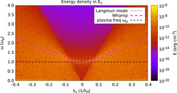
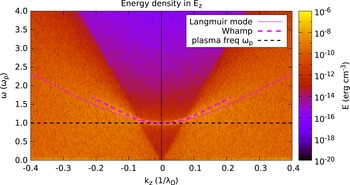
Figure 9 shows the longitudinal electric field,
as determined by the spectral solver that is used in the radiation-free plasma model
as well as the electrostatic plasma model in ACRONYM. The gap at
 $k=0$
is an artefact of the spectral solver that was mentioned before. At
all other
 $k$
the match to the electromagnetic plasma model and the prediction
from theory is very good.
Energy density in the longitudinal component of the electric field. The set-up and parameters are identical to figure 8 but the electric field is computed by the spectral solver that is used in both the radiation-free and the electrostatic plasma model.

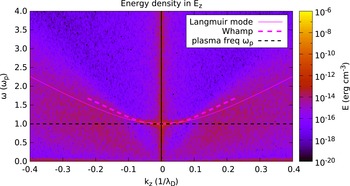
Figure 10 shows the longitudinal electric field
for the alternative implementation of the electrostatic plasma model using the VHS
technique. This method has a very low level of intrinsic noise. To make the Langmuir
mode visible, the initial density of each species was randomly perturbed on every
point of the phase space grid by
 $\pm$
5 %. This reproduces the Langmuir mode at about the same strength as
it appears in the PIC simulations. In the PIC simulations this perturbation is not
necessary, as the Poisson noise in the charge density due to the finite number of
computational particles per cell is sufficient to excite the normal modes of the
plasma on a level that is well visible in the dispersion plots.

Very visible, at least in figures 8 and 9 and still recognizable in figure 10, is the change in the broadband noise floor that is caused by thermal electrons and reaches up to
 $$\begin{eqnarray}\unicode[STIX]{x1D714}=3\sqrt{2}v_{th,e}k.\end{eqnarray}$$
The reduction of this noise floor by at least four orders of magnitude is the main reason to consider implementing the electrostatic plasma model using the VHS method.
The hybrid plasma models do not include kinetic effects of the electrons and assume instantaneous neutrality which, therefore, removes the Langmuir mode as well as the thermal broadband noise.
5.5 Test 5: Bernstein modes
Figure 11 shows the electron Bernstein modes
described in § 3.5. A comparison with
theoretical predictions is hampered by the complicated dispersion relations of these
modes. Using the leading terms of the infinite sums, it is possible to plot the first
few modes. The figure also contains some influence from the
 $X$
mode that has a longitudinal components at low
 $k$
.

Figure 12 shows the behaviour in the
electrostatic model with a static background magnetic field. Again we see a spectral
hole at
 $k=0$
. Compared to figure 11, no
remnants of the
 $X$
mode are visible here.
Energy density in the longitudinal component of the electric field. Unlike figure 11, the field is computed using the spectral solver used by the radiation-free and the electrostatic plasma models.

The absence of kinetic electrons in the hybrid models, carrying individual gyro-phases, removes electron Bernstein modes.
5.6 Test 6: low-frequency
$R$
mode

So far all simulations were as cheap as Test 1. To analyse the low-frequency regime, some more effort is required. Table 4 lists the changes to the simulation parameters.
Energy density in the right-handed circularly polarized part of the electric
field. Similar to figure 6, the
electric field is computed from the electromagnetic plasma model, but this
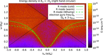
time with the parameters given in tables 1 and 4 to reach the
low-frequency regime. As expected, the low-frequency branch of the
 $R$
mode is visible, including the frequency range of whistler
waves.

Simulation size to study the low-frequency
 $R$
mode.

When we run the simulation using those parameters and plot the result, we again find
the
 $L$
and
 $R$
modes. Limiting ourselves to frequencies up to the electron
gyro-frequency and filtering for right-hand circular polarization, we get
figure 13.
Figure 13 is dominated by the low-frequency
branch of the
 $R$
mode which contains a region where
 $\unicode[STIX]{x1D714}$
depends quadratically on
 $k$
. These waves would usually be classified as whistler waves.
For larger
 $k$
, the group velocity drops again as the wave comes closer to the
resonance at
 $\unicode[STIX]{x1D6FA}_{c,e}$
. In this region, a deviation can be seen between the prediction for
a cold plasma and the mode in the simulated plasma of finite temperature. Using
either the prediction of Chen et al. (Reference Chen, Thorne, Shprits and Ni2013) for a warm plasma or the linearized equations of WHAMP, this effect
can be predicted correctly. Both approaches, however, require the use of a numerical
root finding method. This might seem less elegant than comparison against an analytic
prediction, but root finding codes are quite different to the tested simulation
codes. The risk of implementation problems affecting them in the same way as the
simulation codes is thus minimal and a meaningful comparison can be made.
For even larger
 $k$
, the mode is damped away by gyrating particles, which is also
predicted for warm plasmas. The gyrating electrons generate noise cones around the
electron gyro-frequency that are clearly visible. The opening angle of the cones
corresponds to roughly
 $3\sqrt{2}v_{th,e}k$
.
Figure 14 shows the low-frequency modes that
are right-handed circularly polarized from a radiation-free plasma model. Unlike the
high-frequency branches of
 $L$
and
 $R$
mode that are removed when the electromagnetic radiation is
removed, the low-frequency branches still exist and show the same features as in an
full electromagnetic plasma model.
Energy density in the right-handed circularly polarized part of the electric field. Unlike figure 13 the field is computed using the radiation-free plasma model, but otherwise using the same parameters.

In an electrostatic plasma model, these waves are missing because no transverse fields exist.
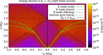
As figure 15 shows, the noise cones of gyrating
electrons – a purely kinetic effect – are missing in a model that uses an electron
fluid. The low-frequency branch of the
 $R$
mode, however, still exists and shows the correct dispersion
relation. This is not surprising as the wave is carried by electrons but exists also
in fluid-like plasma theory. The gyro-frequency of electrons can be estimated from
the spectral gap in the noise.
Energy density in the right-handed circularly polarized part of the electric field. In this figure the field is computed from the hybrid model with electron inertia. Compared to figure 13, the noise cones around the gyro-frequency of electrons are missing.

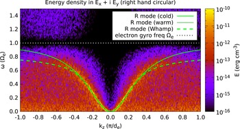
Figure 16 shows the right-hand circular mode in
the limit
 $m_{e}\rightarrow 0$
. For small
 $k$
, the mode is unchanged by the lack of electron inertia, but at
larger
 $k$
it lacks the resonance at the electron gyro-frequency, which is not
well defined without electron mass.
Energy density in the right-handed circularly polarized part of the electric
field. This time a hybrid model with massless electrons is used to compute
the electric field. The dispersion relation of the low-frequency
 $R$
mode is significantly modified by this model as a
comparison with figures 13–15 shows.

Normalizing in the same way as used for the plot
 $\unicode[STIX]{x1D714}=\tilde{\unicode[STIX]{x1D714}}\unicode[STIX]{x1D6FA}_{c,e}$
and
 $k=\tilde{k}\unicode[STIX]{x03C0}/d_{e}$
simplifies the dispersion relation given in (3.23) significantly:
 $$\begin{eqnarray}\tilde{\unicode[STIX]{x1D714}}=\unicode[STIX]{x03C0}^{2}\tilde{k}^{2}.\end{eqnarray}$$
The plot of the spectral energy density indeed shows that the wave
mode follows this dispersion relation even for frequencies
 $\unicode[STIX]{x1D714}$
larger than the electron gyro-frequency.
5.7 Test 7: ion Bernstein modes
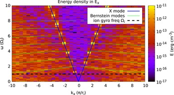
Energy density in the longitudinal component of the electric field. The field has been obtained from the electromagnetic plasma model using the parameter set given in table 5.

Simulation parameters used for the ion Bernstein modes.

Figure 17 shows the result of Test 7 using the
electromagnetic plasma model. The simulation is computationally expensive and quite
noisy. The
 $X$
mode is clearly visible. At smaller phase speeds, ion Bernstein
modes are visible. Better resolution and lower noise levels (e.g. through a larger
number of particles per cell) would be required to make this an efficient test, but
would increase the computational cost even further.
Energy density in the longitudinal component of the electric field. The field has been obtained from the spectral solver used for the radiation-free plasma model.

Figure 18 shows the result of the spectral
solver as used in the radiation-free plasma model. As usual with this solver, a hole
in the spectral energy density appears at
 $k=0$
. This plasma model allows larger time steps than the
electromagnetic model, but the simulation is still too expensive to make an efficient
test problem.
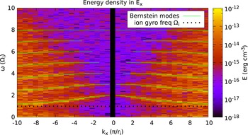
Energy density in the longitudinal component of the electric field. The field has been obtained from the spectral solver used for the electrostatic plasma model using the parameter set given in table 5. The only visible wave modes are ion Bernstein waves.

Figure 19 shows the result of the spectral
solver as used in the electrostatic plasma model. This model does not include the
 $X$
mode and allows much larger time steps, which reduces computational
expense. Additionally, a single time is cheaper than in the radiation-free model and
the test does not rely on the transverse field components that are missing in the
electrostatic model.
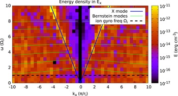
Figure 20 shows the output of the hybrid plasma
model including effects of electron inertia. In this model, ions are treated as
kinetic particles and, as expected, ion Bernstein modes are visible. Note the
reappearance of the
 $X$
mode as an enhanced band of noise at relatively large phase
velocities.
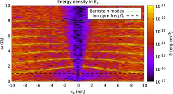
Figure 21 shows the hybrid plasma models without electron inertia. The ion Bernstein modes are dominated by ion kinetic effects and remain unchanged. Given that this plasma model admits a only limited number of modes, this is probably the most relevant test problem for it.
Energy density in the longitudinal component of the electric field. The plot is based on the hybrid model with electron inertia and the parameter set given in table 5.


5.8 Test 8: Low-frequency
$L$
mode

Resolving low-frequency
 $L$
modes, as done in § 5.6 for
their right-handed counterparts, would require another large increase in effort. (One
needs 1836 times as many time steps to resolve the lower gyro-frequency and
 $\sqrt{1836}$
more cells to capture the larger gyro-radius.) The only feasible
way is to reduce the mass ratio between protons and electrons. Low mass ratios result
in possibly unrealistic high Alfvén speeds if the magnetic field is not adjusted.
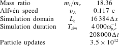
Table 6 shows parameters that are a
reasonable trade-off and allow a glimpse at this wave mode.
Energy density in the left-handed circularly polarized part of the electric
field. The plot is based on a simulation using the electromagnetic plasma
model and parameters given in table 6. As expected, the low-frequency
 $L$
mode is visible as well as noise cones produced by
gyrating ions.

Simulation size to study the low-frequency
 $L$
mode.

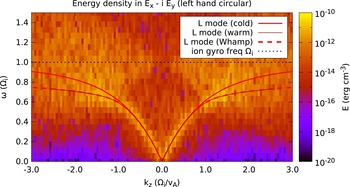
Running the simulation with those parameters and plotting the spectral energy density
of left-handed modes results in figure 22. The
low-frequency branch of the
 $L$
mode is clearly visible. For small
 $k$
, it matches well the prediction for a cold plasma. For intermediate
 $k$
, effects of the finite temperature have to be included to explain
the simulation results. At higher
 $k$
, the mode is damped away by gyrating protons that are visible as
noise cones. These cones are analogous to the cones generated by gyrating electrons,
but occur on ion scales, i.e. they are centred on the gyro-frequency of the ions and
the opening is determined by the thermal speed of ions.
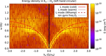
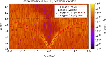
In figure 23 it can be seen that the left-handed low-frequency waves survive in the radiation-free plasma, the same as the right-handed counterparts.
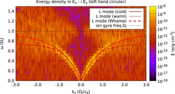
Figures 24 and 25 show that the low-frequency
 $L$
mode branches exist basically unaltered without kinetic electrons.
The noise cones of gyrating ions are unaffected unlike figure 15.
Energy density in the left-handed circularly polarized part of the electric field obtained from the radiation-free plasma model. The simulation parameters can be found in table 6.

Energy density in the left-handed circularly polarized part of the electric
field. Again parameters are from table 6, but this time for a hybrid model with electron inertia. The
ions are still treated kinetically and consequently the low-frequency
 $L$
mode and the noise cones are retained.

Energy density in the left-handed circularly polarized part of the electric field. Compared to figure 24 electron inertia has been removed.

6 Conclusions
In this work we proposed a set of test problems suitable for a wide range of kinetic plasma models and provided reference results based on our numerical codes. Those tests are based on a set of different plasma wave modes and are useful to check quickly and conveniently the correct implementation of different plasma models, including the correct interaction of the different parts of the simulation program handling particles and electromagnetic fields.
Suitability of modes for different plasma models. EB and IB stand for Bernstein
modes of electrons and ions, respectively. Cases indicated by ‘X’ allow for an
effective test. An entry of ‘—’ indicates that the wave mode is not suitable
for testing implementations of this plasma model. The four cases that are
marked $ are in principle suitable, but computationally expensive. The one
special case indicated with
 ${\sim}$
is explained in the text.

Table 7 shows which wave modes are suitable to test codes implementing different plasma models. Listed from left to right are the electromagnetic mode from § 5.1, left- and right-hand circular wave modes at or above the plasma frequency (§ 5.2), the extraordinary mode (§ 5.3), the Langmuir mode (§ 5.4), electron Bernstein modes (§ 5.5), low-frequency waves with right-hand circular polarization (§ 5.6), ion Bernstein modes (§ 5.7) and low-frequency left-hand circular polarization (§ 5.8). Listed on the left-hand side are the different plasma models — from top to bottom —, the electromagnetic model (§ 2.1), the radiation-free model (§ 2.2), the electrostatic model (§ 2.3) and the model using an implicit electron fluid — either with or without electron inertia — described in § 2.4.
Wave modes that provide suitable test problems for the chosen plasma model are indicated
with ‘X’. If a ‘—’ is listed, the wave mode is not present or usable in the plasma
model. For two plasma models, the low-frequency left-hand circularly polarized waves and
the ion Bernstein modes are marked with $. These waves do exist in the electromagnetic
and radiation-free plasma model and show the properties expected from cold plasma
theory. In principle, these waves could be used to test the simulation code, e.g. by
extracting the gyro-frequency of ions or the Alfvén velocity. Simulations with
sufficient resolution are, however, computationally very expensive. Given that these
plasma models admit a large number of alternative wave modes, it is better to choose an
alternative test problem unless low-frequency properties of the ions are explicitly
needed. A special case (indicated by ‘
 ${\sim}$
’), occurs for low-frequency right-hand circularly polarized waves in
the hybrid model without electron inertia. As shown in figure 16, such a wave mode does exist, however, the dispersion relation is
modified compared to all other plasma models used here. In particular the resonance at
the electron gyro-frequency is missing, as it has been ordered out of the model and
cannot be used for comparison purposes. Using the modified dispersion relation in (3.23), it is possible to recover the
combination of magnetic field and electron density. Given the limited number of suitable
wave modes in this hybrid plasma model, right-hand circularly polarized waves are still
an important test problem, but analysis requires extra attention, and direct comparison
with other plasma models is difficult.
Acknowledgements
We acknowledge the use of the ACRONYM code and would like to thank the developers (Verein zur Förderung kinetischer Plasmasimulationen e.V.) for their support. The implementation of the hybrid model is based on a combination with the EMHD code of N. Jain. The authors would like to thank him for all the work on the joint code and all the useful discussion on hybrid plasma models. P.A.M. acknowledges financial support by the Max-Planck–Princeton Center for Plasma Physics. This work is based upon research supported by the National Research Foundation and Department of Science and Technology. Any opinion, findings and conclusions or recommendations expressed in this material are those of the authors and therefore the NRF and DST do not accept any liability in regard thereto.