1. INTRODUCTION
The bump-on-tail instability is one of the most fundamental and basic instabilities in plasma physics. A discussion of this problem, the non-linear evolution of this instability, and the formation and dynamics of coherent structures involving phase-space vortices have been presented in several publications (see, for instance, the recent works of Schamel, Reference Schamel2000; Umeda et al., Reference Umeda, Omura, Yoon, Gaelzer and Matsumoto2003; Eliasson and Shukla, Reference Eliasson and Shukla2006, and references therein). Some early numerical simulations have demonstrated that the dominant stabilization mechanism for the bump-on-tail instability appeared to be the particle trapping in coherent phase-space vortices which develop out of the evolution of an initially unstable perturbation (see for instance Berk, & Roberts, Reference Berk and Roberts1967; Dawson & Shanny, Reference Dawson and Shanny1968; Denavit & Kruer, Reference Denavit and Kruer1971; Joyce et al., Reference Joyce, Knorr and Burns1971; Cheng & Knorr, Reference Cheng and Knorr1976). The use of accurate numerically non-diffusive Eulerian codes (Cheng & Knorr, Reference Cheng and Knorr1976), for the solution of the Vlasov–Poisson system [see Eqs. (1–3) below], has made it possible to present more accurate pictures of the non-linear evolution of the bump-on-tail instability due to an initially unstable wave perturbation (Shoucri, Reference Shoucri1979), where it was demonstrated that the initial bump in the tail of the distribution is distorted during the instability, leading to a state having another bump in the tail of the distribution function, with a minimum of zero slope at the phase velocity of the wave (in this way the large amplitude wave can oscillate at constant amplitude without growth or damping), and with the formation of vortex structures in the phase space which are Bernstein–Greene–Kruskal (BGK) structures (Bernstein et al., Reference Bernstein, Greene and Kruskal1957), traveling at the phase velocity of the wave. These BGK structures have been also observed and discussed in several simulations (see for instance Bertrand et al., Reference Bertrand, Ghizzo, Feix, Fijalkow, Mineau, Suh, Shoucri and Doveil1988; Ghizzo et al., Reference Ghizzo, Izrar, Bertrand, Fijalkow, Feix and Shoucri1988a ; Buchanan & Dorning, Reference Buchanan and Dorning1995; Nakamura & Yabe, Reference Nakamura and Yabe1999; Schamel, Reference Schamel2000; Eliasson & Shukla, Reference Eliasson and Shukla2006; Crouseilles et al., Reference Crouseilles, Respaud and Sonnendrücker2009).
Many of these simulations were executed with the target of providing information while making the codes as economic as possible, i.e. with a grid in space and velocity space as economic as possible, bearing in mind the limitations of the computers and the possibility of extending the methods to higher dimensions. During the evolution of the system, once the microstructure in the phase space reaches the mesh size, it is smoothed away by numerical diffusion, and is therefore lost. Larger scales appear to be unaffected by the small-scale diffusivity and appears to be treated with good accuracy. This had however important consequences on smoothing out micro-information on trapped particles, and modifying some of the oscillations associated with these trapped particles, and with those particles at the separatrix regions of the vortex structures which evolve periodically between trapping and untrapping states and which can only be accurately studied using a fine-resolution phase-space grid. Numerical grid size effects and small time steps can have important consequences on the accuracy of the number and distribution of the trapped particles, on the long-time behavior of the interaction of particles with waves, on kinetic microscopic processes such as the chaotic trajectories which appear in the resonance region at the separatrix of the vortex structures, and for their possible consequences on the large-scale dynamics, as has been pointed out in several publications (see for instance Califano et al., Reference Califano, Pegoraro and Bulanov2000; Doveil et al., Reference Doveil, Firpo, Elskens, Guyomarc'h, Poleni and Bertrand2001; Valentini et al., Reference Valentini, Carbone, Veltri and Mangeney2005; Shoucri, Reference Shoucri and Shoucri2010, Reference Shoucri and Angermann2011). The numerous non-linear effects which accompany the wave–plasma interaction, the wave–wave interaction, and the changing of the distribution functions makes the self-consistent solution of these problems a complicated challenge (Elskens & Escande, Reference Elskens and Escande2003, see also the recent work of Besse et al., Reference Besse, Elskens, Escande and Bertrand2011).
In addition, when the length of the system L is greater than the wavelength λ of the initially unstable wave, unstable sideband modes with longer wavelengths can be excited and grow from round-off errors (Kruer et al., Reference Kruer, Dawson and Sudan1969; Shoucri, Reference Shoucri1978, Reference Shoucri1980, Reference Shoucri2006, Reference Shoucri and Shoucri2010, Reference Shoucri and Angermann2011; Brunetti et al., Reference Brunetti, Califano and Pegoraro2000). Using a high beam density of 10% of the total density, n b = 0.1 in Shoucri (Reference Shoucri and Shoucri2010, Reference Shoucri and Angermann2011), the evolution of the system showed how the onset of the sidebands instability disrupts the BGK equilibrium formed, changes the asymptotic evolution, and bring the system through an inverse cascade of energy, to another state characterized by the formation of distribution functions with inflection points of zero slope appearing at the dominant phase velocities, with localized trapped electron deficit in the phase-space density and cavity-like structures in the density plots. In this case, the use of a fine grid is imperative to follow with accuracy the growth and saturation of the sidebands and to study their effect on the time history which follows the modification of the BGK structures and the formation of the electron phase-space holes. Results presented in Shoucri (Reference Shoucri and Shoucri2010, Reference Shoucri and Angermann2011) show that lower wavenumber modes are driven up by energy cascading to the longer wavelengths, which can have frequencies below the plasma frequency and higher phase velocities than the intermediate BGK wave. Electrons are accelerated to energies in excess of the initial beam energy.
Important results mentioned in the preceding paragraphs are connected: the formation of trapped electron deficit or holes in the phase-space density, associated with the formation of inflection points of zero slope in the spatially averaged distribution function, the existence of dominant waves in the longest wavelengths at frequencies below the plasma frequency. For the problem of electron holes in phase space, a tutorial review has been recently presented by Hutchinson (Reference Hutchinson2017) (and references therein). It offers an interesting review of the widespread occurrence of electron holes in numerical simulations, space-craft observations, and laboratory experiments. Figure 2 of Hutchinson (Reference Hutchinson2017) represents the results obtained for the formation of an electron hole from a simulation using the one-dimensional (1D) particle-in-cell (PIC) code XES1, distributed with the textbook of Birdsall and Langdon (Reference Birdsall and Langdon1991). In this simulation, two electron streams of opposite velocity and equal density give rise to instability. The wave grows until a non-linear BGK regime of four vortices is formed, but they merge rapidly (the PIC code is usually sufficiently noisy), until a single hole is left, associated with a positive potential at the position of the hole. The underlying theory for the electron hole is of a 1D localized potential maximum self-consistently sustained by a deficit of trapped electron phase-space density. This illustrates the fact that essentially any collisionless two-stream instability in 1D gives rise to electron holes. Indeed, electron holes have been also obtained in the long-time limit of the bump-on-tail instability, as mentioned in the previous paragraph, using the computational power of an Eulerian Vlasov code (Shoucri, Reference Shoucri and Shoucri2010, Reference Shoucri and Angermann2011). These results obtained for the electron holes are at a velocity about five times the thermal speed, in the low-density region of the plasma [while the results obtained using a PIC code by Birdsall and Langdon (Reference Birdsall and Langdon1991) are in the bulk of the distribution function, to overcome the problem of the numerical noise in the low-density region of the electron distribution function inherent in PIC simulations]. Note also in the results in Figure 7 of Shoucri (Reference Shoucri and Angermann2010), the study of two electron holes merging together, in the low-density region at a velocity about five times the thermal speed of the electron distribution function (which to our knowledge is reported for the first time). The results do confirm the elementary underlying theory reviewed in Hutchinson (Reference Hutchinson2017), of a 1D electron hole at a localized potential maximum, self-consistently sustained by a deficit of trapped electron phase-space density [see Fig. 23 of Shoucri (Reference Shoucri and Angermann2010)], where the negative of the electric field and the negative of the potential are plotted, and Figure 24 for the electron density shows clearly a deficit of the electron density at the location of the electron hole.
An important result we mentioned above is the formation of inflection points of zero slope in the electron distribution function, at the dominant waves phase velocities. These phase velocities in our case are about five times the thermal speed, in the low-density region of the distribution function, and at frequencies below the plasma frequency. We note that a study of distribution functions with inflection points of zero slope has been recently presented by Valentini et al. (Reference Valentini, Perrone, Califano, Pegorare, Veltri, Morrison and O'Neil2012), in a study of undamped waves in plasmas that are small amplitude limit of non-linear excitations, such as electron acoustic waves (EAWs), and where the distribution functions have a small deviation consisting of a very small plateau with zero velocity derivative. However, the phase velocities of these waves are of the order of the thermal speed. An EAW is a BGK mode with a velocity distribution function that is effectively flat at the wave phase velocity. Holloway and Dorning (Reference Holloway and Dorning1991), Demeio and Holloway (Reference Demeio and Holloway1991), Shadwick and Morrison (Reference Shadwick and Morrison1994) have shown that stationary inflection point modes are linear limits of the EAWs. A stationary inflection point mode is a mode with a phase velocity at a point where the first two derivatives of a stable homogeneous equilibrium velocity distribution function vanish. This is a necessary and sufficient condition for the stability of the mode according to the Penrose criterion. These EAWs can exist on the so-called thumb dispersion relation (Demeio & Holloway, Reference Demeio and Holloway1991; Sircombe et al., Reference Sircombe, Arber and Dendy2006; Valentini et al., Reference Valentini, O'Neill and Dubin2006). These waves can also be obtained off the dispersion curve (Yin et al., Reference Yin, Daughton, Albright, Bezerrides, DuBois, Kindel and Vu2006; Strozzi et al., Reference Strozzi, Williams, Langdon and Bers2007, Reference Strozzi, Williams, Langdon, Bers, Brunner and Shoucri2010; Valentini et al., Reference Valentini, Perrone, Califano, Pegorare, Veltri, Morrison and O'Neil2012). In the study presented by Valentini et al. (Reference Valentini, Perrone, Califano, Pegorare, Veltri, Morrison and O'Neil2012), the alteration of the distribution function is done by replacing the trapped particle region by a plateau and by using a simple linear dispersion analysis to analyze the stability of the system. The focus was on relatively low amplitude EAWs, either on-dispersion or off-dispersion curve, where non-linearity is limited to a narrow velocity range of trapped particles, and the phase velocity is of the order of the thermal speed. We see that the thumb curve of Holloway and Dorning (Reference Holloway and Dorning1991) is of limited predictive capability.
Another important result we mentioned in the preceding paragraphs is the appearance of dominant waves at frequencies below the plasma frequency at the longest wavelengths available. The present work makes a connection between the existence of a localized electron deficit in the phase-space density associated with a self-consistent positive potential at the position of the hole, an inverse cascade where energy is cascading to the lowest wavenumbers available and where wave frequencies below the plasma frequency are appearing; and finally inflection points of zero slope of the electron distribution function at the phase velocities of the dominant waves, at about five times the thermal speed. In the present work, we use an Eulerian Vlasov code to study the long-time non-linear evolution of a bump-on-tail instability with a beam density 10% of the plasma density. We use a fine grid in phase space and time step in this case of large amplitude initial perturbation and strong beam–plasma interaction, where the initial beam density is n b = 0.1. The instability evolves and leads to the formation of a BGK structure, which now is an intermediate regime. When the system length L is greater than the wavelength λ of the unstable mode, sidebands will next grow from round-off errors and will dominate and disrupt the BGK structure, and in the asymptotic state the distribution function coming out of the evolution of the energy cascading to the lowest wavenumbers available, has inflection points of zero slope at the phase velocities of the dominant modes, at frequencies below the plasma frequency. In Shoucri (Reference Shoucri and Shoucri2010, Reference Shoucri and Angermann2011), the length and parameters were such that the lowest wavenumber available was the fundamental mode, with a phase space and a density plot showing a single cavity structure, and two distinct holes formed merged subsequently in a single one. The noiseless Vlasov code allowed to follow in details this merging of holes, taking place at about five times the thermal speed, in the low-density region of the phase space. In the case, we present in this work, however, the dominant asymptotic state is the harmonic n = 2, which results in a phase space and a density plot showing two cavity structures, even symmetry is conserved and even harmonics dominate during the evolution of the system. The odd harmonics remained negligibly small. This diversity of results indicates a variety of solutions to this problem. We note that Siminos et al. (Reference Siminos, Bénisti and Grémillet2011) have studied the stability of BGK modes and showed that under certain conditions of length and parameters, the instability of the n = 2 harmonic would dominate.
2. THE RELEVANT EQUATIONS
The relevant equations are the 1D Vlasov equation for the electron distribution function f(x, υ, t), coupled to the Poisson equation. Ions form an immobile background. These equations are written in our normalized units:
 $$\displaystyle{{\partial f} \over {\partial t}} + {\rm \upsilon} \displaystyle{{\partial f} \over {\partial x}} - E_x\displaystyle{{\partial f} \over {\partial {\rm \upsilon}}} = 0$$
 $$\displaystyle{{\partial ^2{\rm \phi}} \over {\partial x^2}} = - (1 - n_{\rm e}(x));\quad n_{\rm e}(x) = \int\limits_{ - \infty} ^{ + \infty} {\,f\,(x,{\rm \upsilon} ){\rm d}{\rm \upsilon}} $$
 $$E_x = - \displaystyle{{\partial {\phi}} \over {\partial x}}$$
Time t is normalized to the inverse electron plasma frequency
 ${\rm \omega} _{{\rm pe}}^{-1} $
, velocity is normalized to the electron thermal velocity υth and length is normalized to the Debye length λD = υth/ωpe. Equation (3) relates the electric field and the potential. Periodic boundary conditions are used. These equations are discretized on a grid in phase space and are numerically solved with an Eulerian code, by applying a method of fractional step which has been previously presented and widely applied for the numerical solution of these set of equations for a widely varied set of problems rich in physics (we cite, for instance, Cheng & Knorr, Reference Cheng and Knorr1976; Shoucri, Reference Shoucri1978; Reference Shoucri1979, Reference Shoucri1980, Reference Shoucri2008, Reference Shoucri, Colombo and Rizzo2009; Shoucri & Storey, Reference Shoucri and Storey1986; Califano & Lantano, Reference Califano and Lantano1999; Brunetti et al., Reference Brunetti, Califano and Pegoraro2000; Pohn et al., Reference Pohn, Shoucri and Kamelander2005; Califano et al., Reference Califano, Galeotti and Mangeney2006; Umeda, Reference Umeda2008; Arber et al., Reference Arber, Sircombe, Vann and Shoucri2011). We write the main steps to advance Eq. (1) by a time-step Δt from a time t to a time t + Δt:
 $${\rm Step 1:\, Solve}\,\,\displaystyle{{\partial f} \over {\partial t}} + {\rm \upsilon} \displaystyle{{\partial f} \over {\partial x}} = 0\,\,{\rm for}\,{\rm a} \,{\rm step}\,\,\Delta t/2$$
Solve Poisson equation in Eq. (2) for the electric field which we denote by
 $E_x^\ast $$
.
 $${\rm Step 2:\, Solve}\,\,\displaystyle{{\partial f} \over {\partial t}} - E_x^\ast \displaystyle{{\partial f} \over {\partial {\rm \upsilon}}} = 0\,\; {\rm for \,a \,step}\,\Delta t$$
 $${\rm Step 3: Solve}\,\,\displaystyle{{\partial f} \over {\partial t}} + {\rm \upsilon} \displaystyle{{\partial f} \over {\partial x}} = 0\,\,{\rm for \,a \,step}\,\Delta t/2$$
Each of the x or υ updates is solved by a linear advection done by applying successively the following shifts:
 $$f^a(x,{\rm \upsilon}, t + \Delta t/2) = f\,(x - {\rm \upsilon} \Delta t/2,{\rm \upsilon}, t)$$
 $$f^b(x,{\rm \upsilon}, t + \Delta t) = f\,(x,{\rm \upsilon} - E_x^\ast \Delta t,t)$$
 $$f\,(x,{\rm \upsilon}, t + \Delta t/2) = f^b(x - {\rm \upsilon} \Delta t/2,{\rm \upsilon}, t)$$
The shifts in Eqs. (7–9) are calculated using a cubic spline interpolation. For further details, see for instance Cheng and Knorr (Reference Cheng and Knorr1976), Gagné and Shoucri (Reference Gagné and Shoucri1977), Pohn et al. (Reference Pohn, Shoucri and Kamelander2005), and Shoucri (Reference Shoucri2008).
3. THE BUMP-ON-TAIL INSTABILITY
The distribution function of a homogeneous beam-plasma system, with a small-density electron beam drifting with a velocity υd relative to a stationary homogeneous plasma is given by:
 $$f\,({\rm \upsilon} ) = \displaystyle{{n_{\rm p}} \over {\sqrt {2{\rm \pi}}}} {\rm e}^{ - 1/2{\rm \upsilon} ^2} + \displaystyle{{n_{\rm b}} \over {\sqrt {2{\rm \pi}} {\rm \upsilon} _{{\rm thb}}}}{\rm e}^{ - 1/2({\rm \upsilon} - {\rm \upsilon} _{\rm d})^2/{\rm \upsilon} {_{{\rm thb}}^2} }$$
We take for the plasma density n p = 0.9 and for the beam density n b = 0.1 for a total density of 1. The ions form an immobile background of density 1. The beam thermal spread is υthb = 0.5. We perturb the system initially with a perturbation such that:
 $$f\,(x,{\rm \upsilon} ) = f\,({\rm \upsilon} )(1 + {\rm \varepsilon} \cos (kx))$$
with ε = 0.04 and with k = n2π/L, and f(υ) is given in Eq. (10). We consider the case where a single mode with k = 0.3 is initially perturbed, and the approximate initial frequency response of the system will be ω2 ≈ 1 + 3k 2, or ω ≈ 1.127, with an initial phase velocity of the wave ω/k = 3.756. This phase velocity corresponds to a velocity where the initial distribution function in Eq. (10) has a positive slope. Hence the perturbation in Eq. (11) will lead to an instability. We study the case where the mode k = 0.3 corresponds to the harmonic n = 6. Since k = n2π/L = 0.3, then the length of the system in this case is L = 40π, in which case unstable sidebands can grow and modify the BGK vortex structures of the phase space (the length of the system is bigger with respect to the wavelength of the excited oscillation).
4. EXCITATION OF A HARMONIC MODE N = 6 WITH K = 0.3
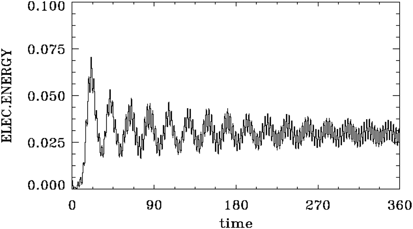
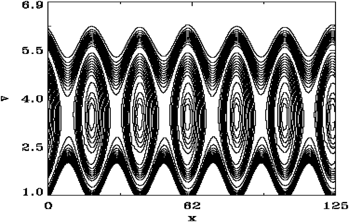
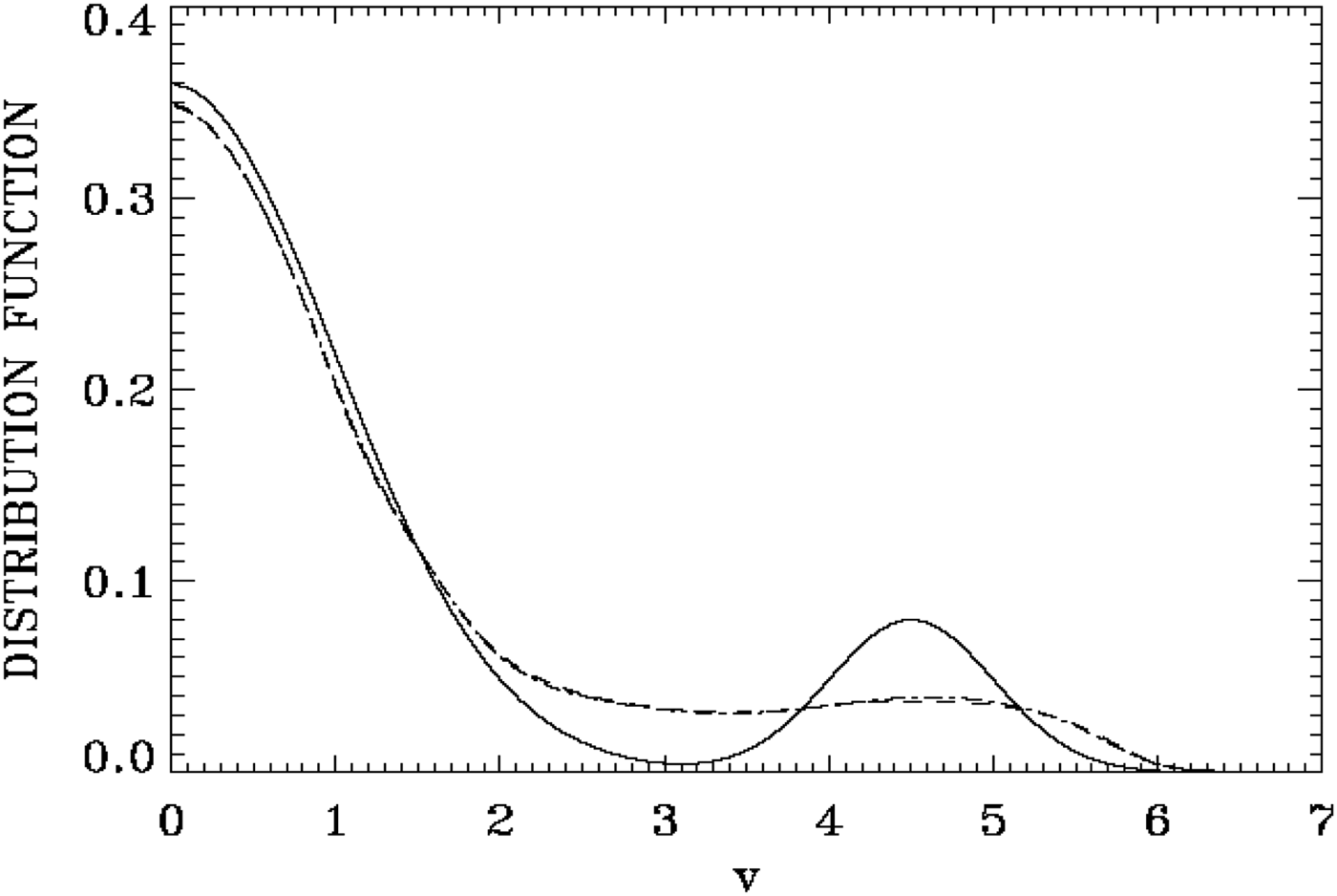
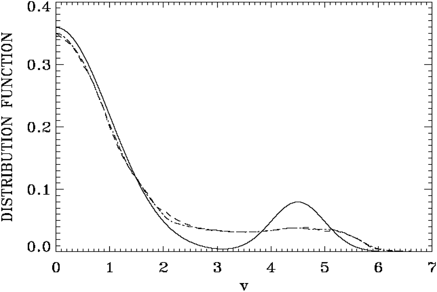
In a first simulation, we use the initial perturbation as in Eq. (11). We first present the results obtained using a space-velocity grid of 256 × 256, and a time step Δt = 0.05. With extrema of the velocity at ± 7, the recurrence time for the excited wave is τ = 2π/kΔυ = 381. Figure 1 shows the time evolution of the electric energy, essentially resulting from the initially unstable mode with n = 6, up to t = 360. It shows growth, saturation, and then the modulation due to the trapped particles. The electric energy seems to evolve to a constant value with the superimposed oscillation at the plasma frequency. Figure 2 shows the phase space at t = 340, where we concentrate the plot around the BGK structure of six vortices which are formed after the saturation of the initial bump-on-tail instability (note the smooth contours of the equilibrium). Figure 3 presents the spatially averaged distribution function:
 $$F({\rm \upsilon} ) = \displaystyle{1 \over L}\int\limits_0^{\rm L} {\,f\,(x,{\rm \upsilon} ){\rm d}x} $$
initially at t = 0 (full curve), at t = 320 (dashed curve), and at t = 360 (dashed-dotted curve).
Time evolution of the electric energy for the case of a 256 × 256 grid points.

Phase space of the distribution function in the region of the vortices at t = 340 for the case of a 256 × 256 grid points.

Spatially averaged distribution function f(υ) at t = 0 (full curve), t = 320 (dashed curve), and t = 360 (dashed-dotted curve) for the case of a 256 × 256 phase-space grid points (the dashed and dashed-dotted curves overlap).

The initial bump on tail has evolved at t = 360 to another smooth bump on tail with a minimum of zero slope around υ ≈ 3.5. With a non-linear measured frequency of ω ≈ 1.06, this corresponds to the phase velocity of the wave 1.06/0.3 = 3.53, essentially at the minimum we see in Figure 3 at t = 360, so the wave can oscillate at a constant amplitude. The BGK structure in Figure 2 has its center at a velocity about 3.5, so the BGK structure is traveling at the phase velocity of the wave. These results are similar to what is presented for a similar problem in the literature previously cited in section 1 in Introduction. When the simulation is stopped at t = 360, sidebands remained small and did not affect the BGK equilibrium in Figure 2.
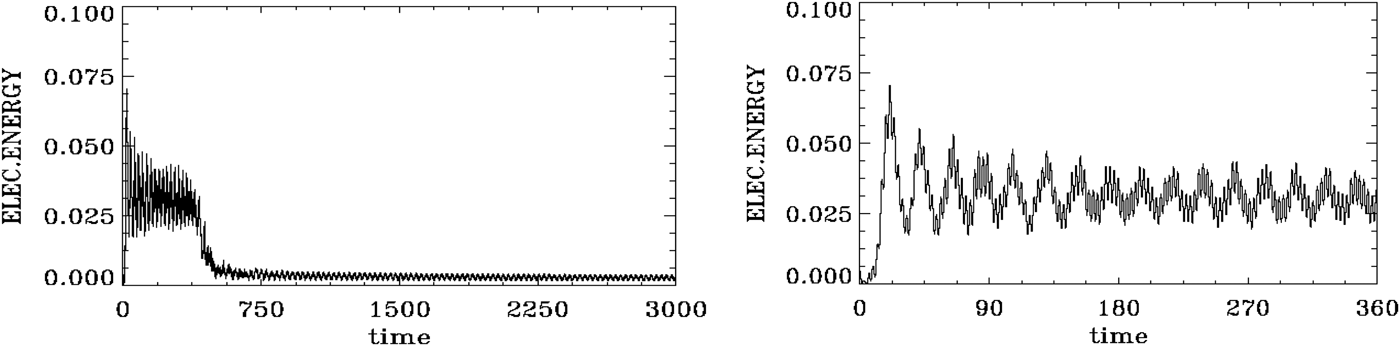
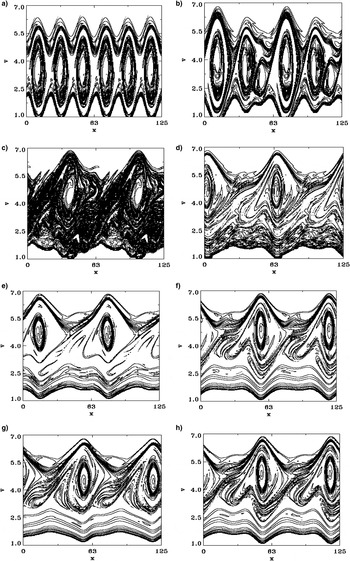
The results obtained in a second simulation with a phase-space grid of 1024 × 2400 points have another story. With the same extrema of the velocity at ± 7, the recurrence time for the unstable mode with k = 0.3 is τ = 2π/kΔυ = 3588. We use Δt = 0.002. We use the same initial perturbation as in Eq. (11). Figure 4a presents the time evolution of the electric energy, essentially resulting from the initially unstable mode with n = 6, showing growth, saturation, and trapped particle oscillations. We present the same results up to t = 360 in Figure 4b, to facilitate a comparison with Figure 1. Starting from the sixth or seventh peak in Figure 4b, it is clear that the modulation due to the trapped particles oscillation is more important in Figure 4b with respect to Figure 1. Unstable sidebands, with n = 1,2,3,4,5 or n = 7,8,9,10,11 for instance, growing from round-off errors, are now completely modifying the evolution of the system around and after t ≈ 370, when they reach a level where they disrupt the BGK equilibrium. Figure 5 shows the spatially averaged distribution function at t = 0 (full curve), at t = 320 (dashed curve) and at t = 360 (dashed-dotted curve), close to what is presented in Figure 3. It shows a minimum around υ ≈ 3.5, at the phase velocity of the wave. However, differences in the phase-space contour plots can be seen by comparing Figure 2 with Figure 6a obtained at t = 320. Note the important details of the trapped particles in Figure 6a, and on the top of the six vortices, we see a small layer of another population of trapped particles. The sharp decay in the electric energy in Figure 4a around t ≈ 370 shows the effect when the growing sidebands disrupt the BGK equilibrium. The electric energy in Figure 4a shows a rapid decay to another constant level, which is also modulated by the trapped particles. This drop in the electric energy level is accompanied by an acceleration of particles to higher velocities.
(a) Time evolution of the electric energy for the case of a 1024 × 2400 grid points (left frame); (b) same in as (a), plotted until t = 360 (right frame).

Spatially averaged distribution function f(υ) at t = 0 (full curve), t = 320 (dashed curve), and t = 360 (dashed-dotted curve) for the case of a grid of 1024 × 2400 points.

Phase-space plot of the distribution function in the region of the holes at: (a) t = 320, (b) t = 400, (c) t = 500, (d) t = 1000, (e) t = 2000, (f) t = 2920, (g) t = 2960, (h) t = 3000.

The subsequent evolution of the phase space is shown in Figure 6b–6h at t = 400, 500, 1000, 2000, 2920, 2960, and 3000, respectively. It shows the fusion of the vortices and the transition of the structure from six to two vortices, whose details are sensitive to the fine-grid resolution. Note in these figures how the rather strong disruption of the BGK equilibrium and the fusion of the vortices is taking place preserving during the evolution the even symmetry of the resulting dominant n = 2 mode. Statistical physics of 2D systems (Knorr, Reference Knorr1977) shows that energy should flow by inverse cascade to the longest wavelength available in the system. The inverse cascade in the present case takes place in such a way that the even symmetry of the system is conserved, that is, only even modes dominate in the asymptotic state. In the results presented in Shoucri (Reference Shoucri and Shoucri2010, Reference Shoucri and Angermann2011), we observe the merging of two holes into a single one. In the present simulation, the odd modes saturated at much lower levels than the even modes (as we shall see in more details below in Figures 11–22), and consequently the dominant mode at the end was the n = 2 mode, and not the fundamental n = 1 mode. Even when the n = 1 and n = 3 modes were given an initial perturbation in order to enhance their growth, they saturated at a low level leaving the even symmetry unchanged. Results presented by Siminos et al. (Reference Siminos, Bénisti and Grémillet2011), who studied the stability of the BGK modes, have also pointed to cases where under certain conditions of length and parameters, the instability of the n = 2 mode dominates. We also note that the centers of the holes in Figure 6d–6h have moved upward with respect to the result in Figure 6a, as a result of the acceleration of the particles to higher velocities. A small vertical oscillation of the center of the holes is present in Figure 6f–6h. The period of this oscillation is about 80, and is taking place around the velocity value of υ = 4.697, which is the phase velocity of the dominant n = 2 mode (see Discussion below). In addition to this vertical oscillation, we have the horizontal translation of the holes at a speed about υ = 4.697, and the gyration or rotation of the structure. More details are given at the end when discussing the different Fourier modes in Figures 11–22.
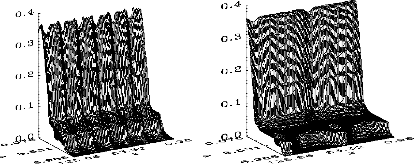
Figure 7a shows the 3D plot of the results in Figure 6a, and Figure 7b shows the 3D plot of the results in Figure 6h. Note the vertical modulation of the bulk of the distribution function in Figure 7a, corresponding to the initially unstable harmonic n = 6, and note in Figure 7b in the horizontal striation or modulation in the bulk of the plasma corresponding to phase velocities of different modes excited.

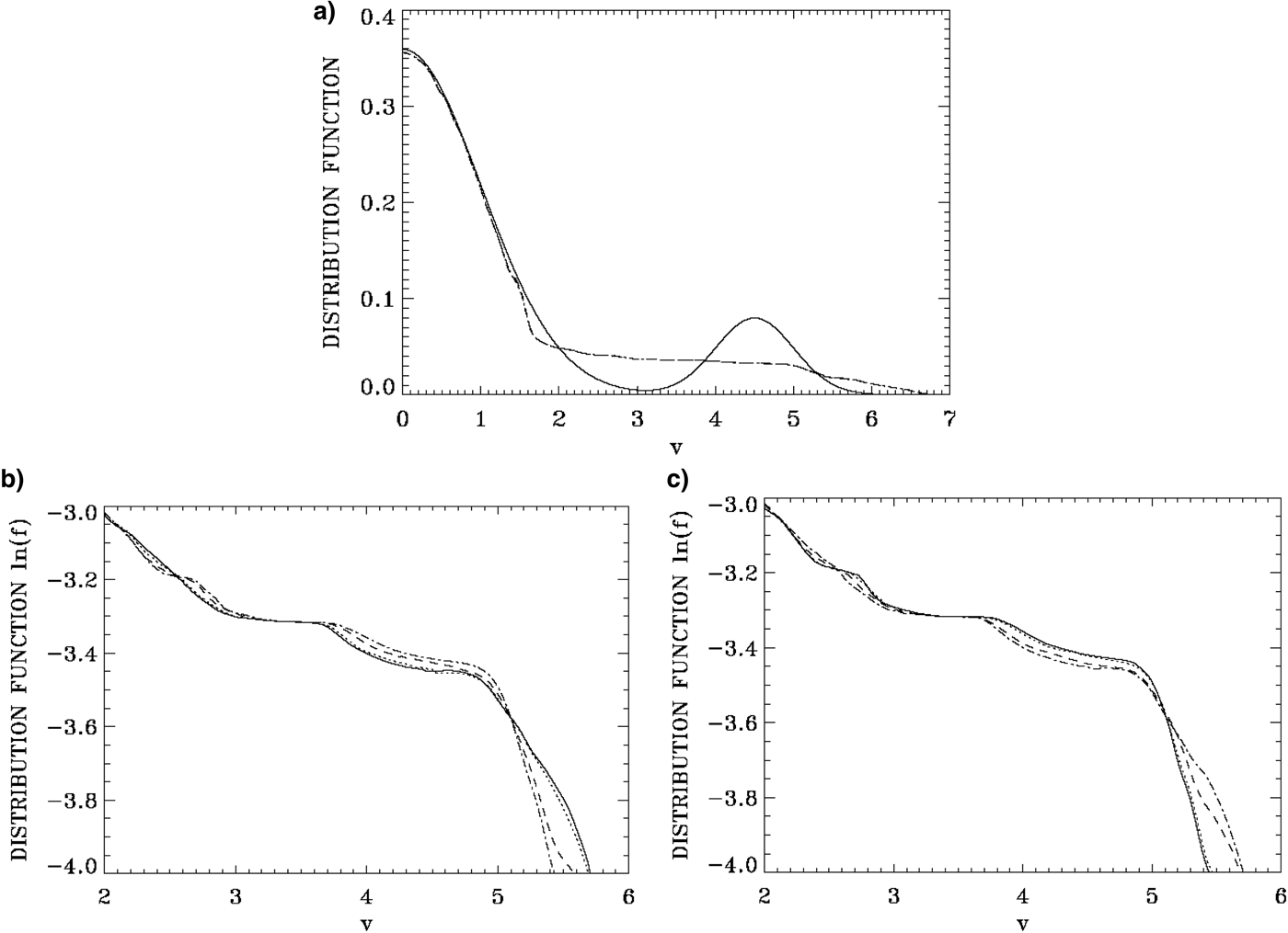
Figure 8a shows the spatially averaged distribution function at t = 0 (full curve), at t = 2920 (dashed curve), and at t = 3000 (dashed-dotted curve). It shows what appears to be a long smoothly decaying tail in the distribution function. More details can be obtained however if we plot the distribution function on a logarithmic scale concentrating on the region of the tail. Figure 8b show the spatially averaged distribution function at t = 2520 (full curve), t = 2540 (dashed curve), t = 2560 (dashed-dotted curve), and t = 2600 (dotted curve). The dotted curve at t = 2600 repeats the full curve at t = 2520. Figure 8c shows the spatially averaged distribution function at t = 2920 (full curve), t = 2940 (dashed curve), t = 2960 (dashed-dotted curve), and t = 3000 (dotted curve). Again the dotted curve at t = 3000 repeats the full curve at t = 2920 (they almost exactly overlap). It is clear that we have here a persistent oscillation in the tail of the distribution function of period about 80, which repeats itself exactly. This oscillation corresponds to the small vertical oscillation of the center of the vortical structure we mentioned before in Figure 6f–6h. The distribution functions in Figure 8b, c show an inflection point or a very small plateau of zero slope around υ = 3.7, and shows a very small oscillation between the inflection point of zero slope and a very small positive slope, taking place around υ = 4.697. These values correspond to phase velocities of the excited dominant modes, as we shall see in details when discussing the different Fourier modes in Figures 11 and 12. A comparison of Figure 8b, c with Figure 6f–6h shows that the vortices appearing in these last figures are located on the decaying part of the distribution functions tail in Figure 8b, c, and the center of the vortices is oscillating, with a period of 80, around the inflection point of zero slope around υ ≈ 4.697.
Spatially averaged distribution function f(υ) at: (a) t = 0 (full curve), t = 2920 (dashed curve), and t = 3000 (dashed-dotted curve); (b) t = 2520 (full curve), t = 2540 (dashed curve), t = 2560 (dashed-dotted curve), and t = 2600 (dotted curve), (c) t = 2920 (full curve); t = 2940 (dashed curve), t = 2960 (dashed-dotted curve), and t = 3000 (dotted curve).

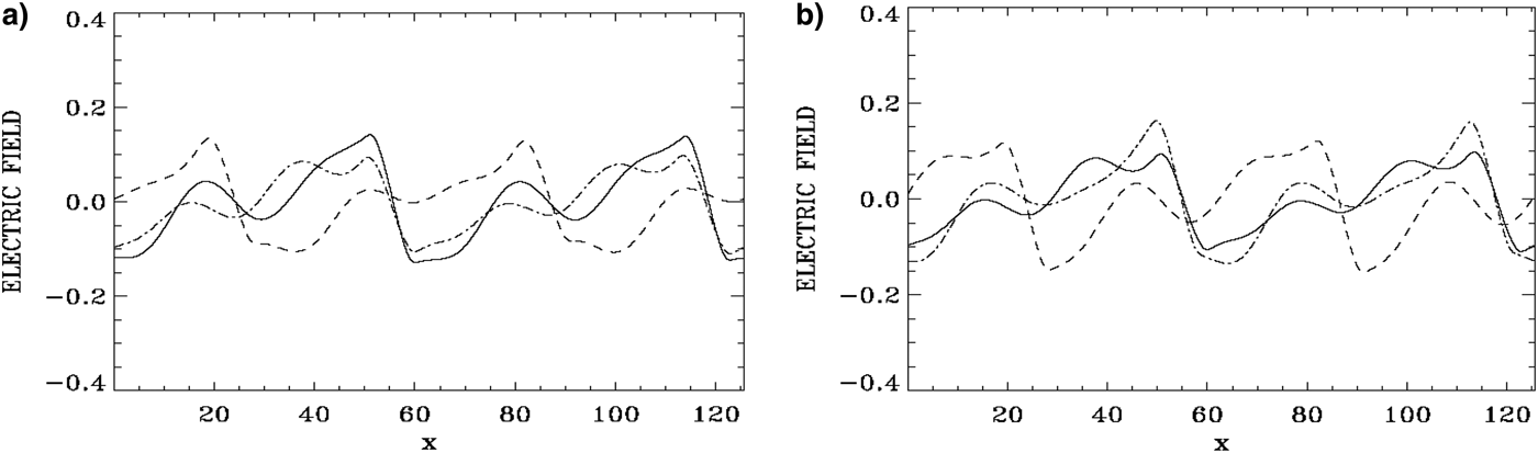
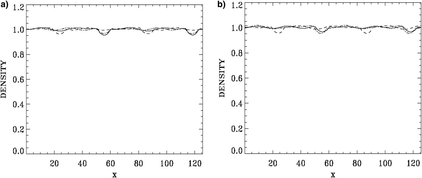
Figure 9a shows the negative E = −E x of the electric field profiles at t = 2920 (full curve), 2940 (dashed curve), and 2960 (dashed-dotted curve), and Figure 9b shows the negative E = −E x of the electric field profiles at t = 2960 (full curve), 2980 (dashed curve), and 3000 (dashed-dotted curve). Figure 10a, b present the corresponding electron density profiles at the same times. Note the localized electron density deficit appearing in the form of two bell-shaped cavities in the present electron density plots, at positions corresponding to the phase-space holes position in Figure 6, which is also the positions where in Figure 9a, b the negative E = −E x of the electric field shows a rapid variation from positive to negative values. This rapid variation of the electric field will translate in the associated potential profile to a solitary-like structure, see for instance Figure 23 in (Shoucri, Reference Shoucri and Angermann2010), where we also plotted E = −E x and the negative of the potential. (Note in Fig. 23 in Shoucri Reference Shoucri and Angermann2010, if we reverse the sign of the electric field and the potential, we get profiles similar to what we see in Fig. 5 of Hutchinson Reference Hutchinson2017.) (This reverse in the electric field sign is simply due to the fact that in the numerical code, Eqs. (1–3) have been solved by substituting E = −E x , a numeric substitution which has no physical significance.)
Electric field profile E = −E x at: (a) t = 2920 (full curve), t = 2940 (dashed curve), t = 2960 (dashed-dotted curve), (b) t = 2960 (full curve), t = 2980 (dashed curve), t = 3000 (dashed-dotted curve).

(a) Electron density profile at t = 2920 (full curve), t = 2940 (dashed curve), t = 2960 (dashed-dotted curve), (b) electron density profile at t = 2960 (full curve), t = 2980 (dashed curve), t = 3000 (dashed-dotted curve).

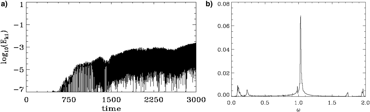
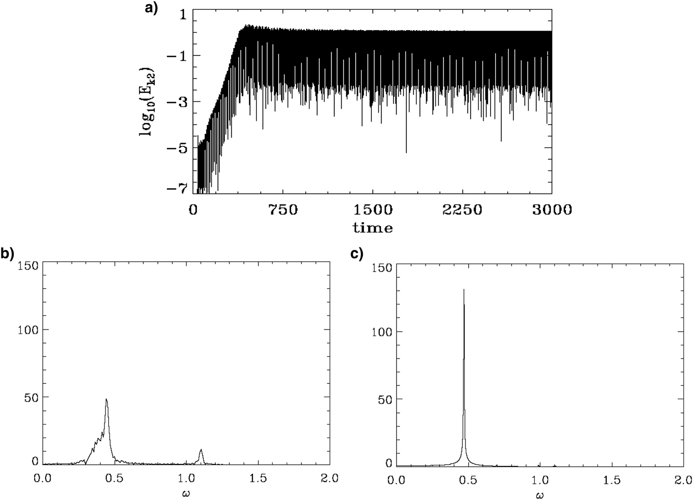
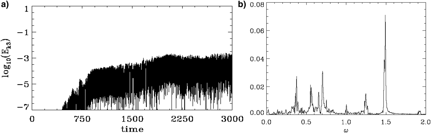
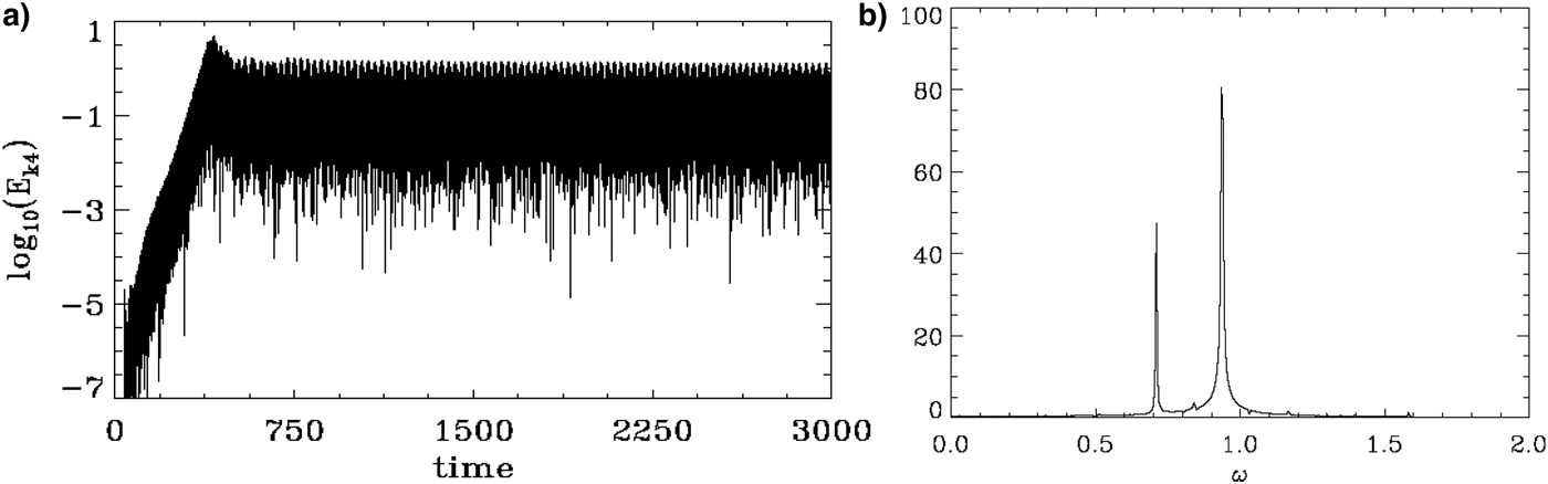
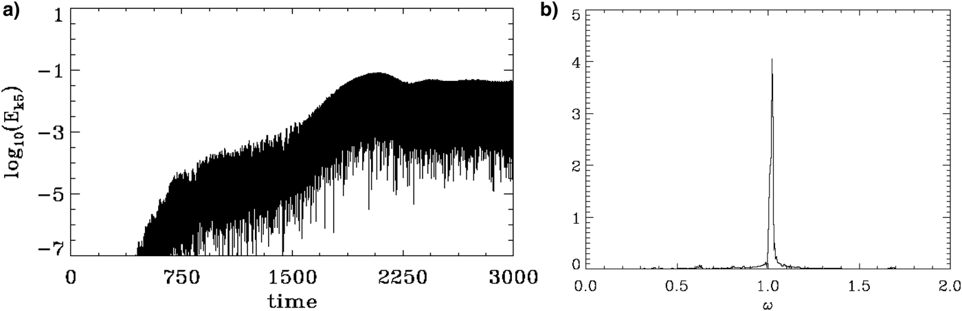
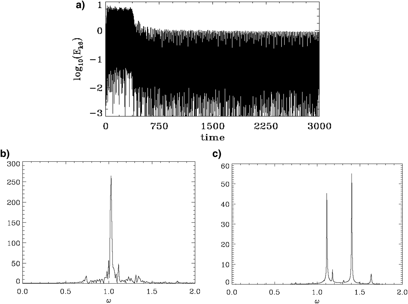
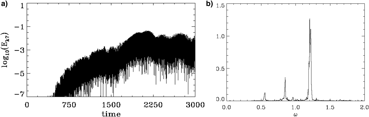
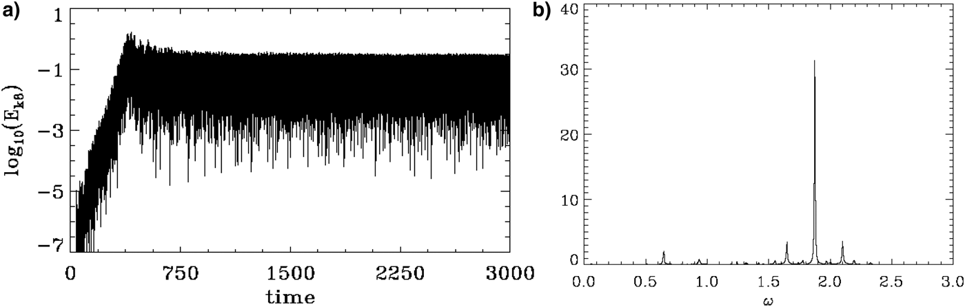
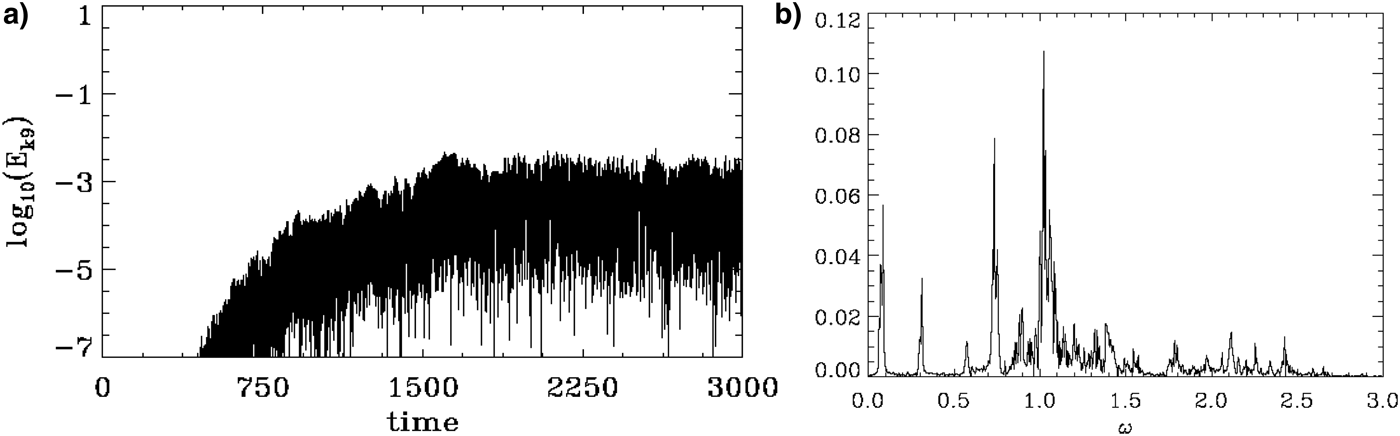
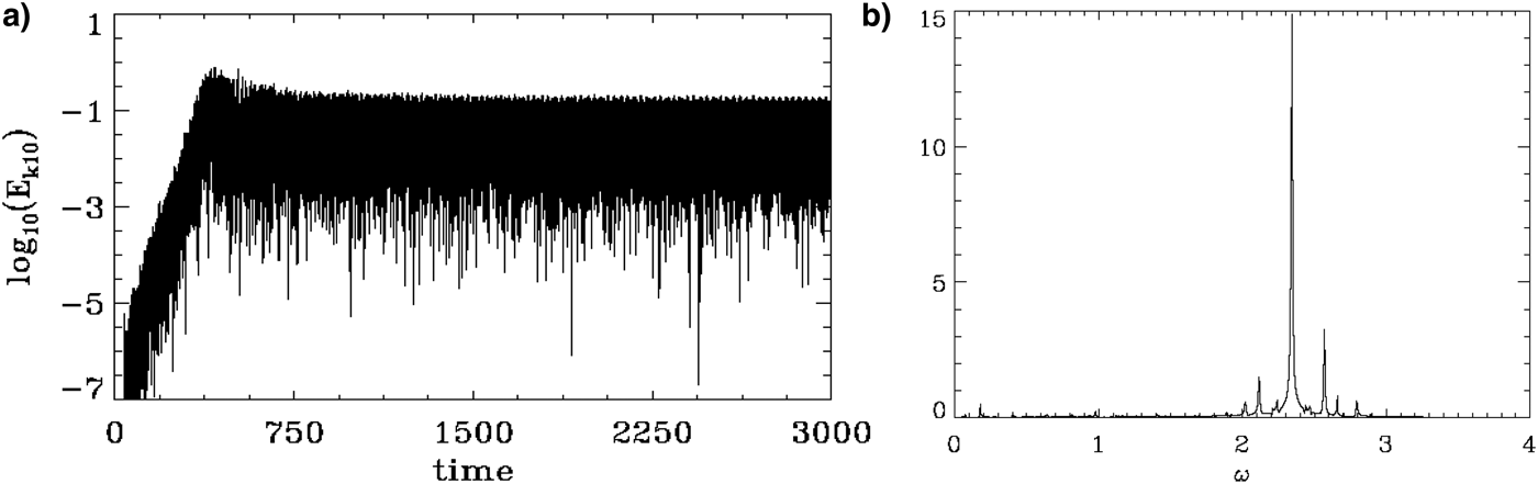
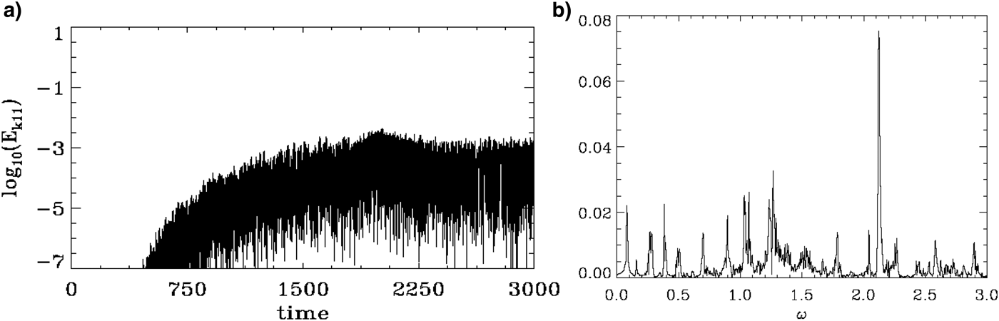
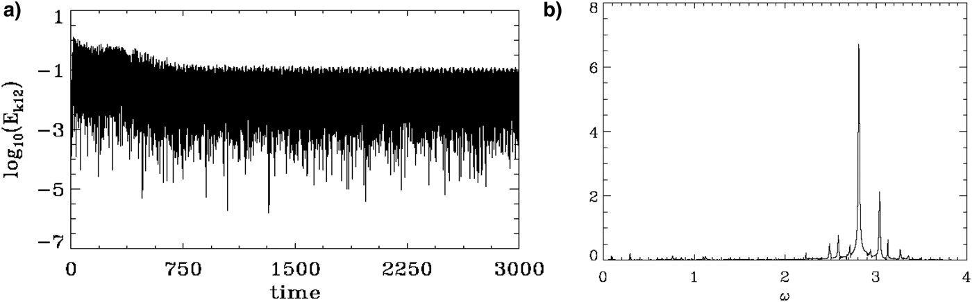
The time evolution of the Fourier modes n = 1–12 are presented in Figures 11–22, respectively, together with the corresponding frequency spectra (note the difference in the vertical scale in these figures). The odd modes n = 1, 3, 5, 7, 9, 11 in Figures 11, 13, 15, 17, 19, 21 remained small, giving small values for their frequency spectra. The time evolution of the mode n = 2 or k = 0.1 is given in Figure 12a and is the dominant mode during the steady-state oscillation as we previously mentioned. The inverse cascade is taking place in such a way that the even symmetry of the system is conserved. The frequency spectrum of the mode n = 2, k = 0.1 is given in Figure 12b during the initial period of growth and early fusion of the vortices, from t 1 = 40 to t 2 = 695. It shows during this period the presence of the growing mode frequency with ω = 0.441, and the decaying initial mode at ω = 1.102. In Figure 12c, the frequency spectrum is calculated during the steady-state oscillation from t = 1689 to t = 3000 at the end of the simulation, and shows a dominant frequency ω = 0.4697, below the plasma frequency. The corresponding phase velocity is υph = 0.4697/0.1 = 4.697, which corresponds to the point where the distribution function in Figure 8b, c is oscillating between a shape with an inflection point of zero slope or very small negative slope appearing around the velocity υ ≈ 4.69.
(a) Time evolution of the Fourier mode n = 1 (k = 0.05), (b) frequency spectrum of the mode k = 0.05, during the steady-state oscillation from t 1 = 1689 until t 2 = 3000 (note the small vertical scale).

(a) Time evolution of the Fourier mode n = 2 (k = 0.1), (b) frequency spectrum of the mode k = 0.1, during the initial phase from t 1 = 40 until t 2 = 695, (c) frequency spectrum of the mode k = 0.1, during the steady-state oscillation from t 1 = 1689 until t 2 = 3000.

(a) Time evolution of the Fourier mode n = 3 (k = 0.15), (b) frequency spectrum of the mode k = 0.15, during the steady-state oscillation from t 1 = 1689 until t 2 = 3000.

(a) Time evolution of the Fourier mode n = 4 (k = 0.2), (b) frequency spectrum of the mode k = 0.2, during the steady-state oscillation from t 1 = 1689 until t 2 = 3000.

(a) Time evolution of the Fourier mode n = 5 (k = 0.25), (b) frequency spectrum of the mode k = 0.25, during the steady-state oscillation from t 1 = 1689 until t 2 = 3000.

(a) Time evolution of the Fourier mode n = 6 (k = 0.3), (b) frequency spectrum of the mode k = 0.3, during the initial phase from t 1 = 40 until t 2 = 695, (c) frequency spectrum of the mode k = 0.3, during the steady-state oscillation from t 1 = 1689 until t 2 = 3000.

(a) Time evolution of the Fourier mode n = 7 (k = 0.35), (b) frequency spectrum of the mode k = 0.35, during the steady-state oscillation from t 1 = 1689 until t 2 = 3000.

(a) Time evolution of the Fourier mode n = 8 (k = 0.4), (b) frequency spectrum of the mode k = 0.4, during the steady-state oscillation from t 1 = 1689 until t 2 = 3000.

(a) Time evolution of the Fourier mode n = 9 (k = 0.45), (b) frequency spectrum of the mode k = 0.45, during the steady-state oscillation from t 1 = 1689 until t 2 = 3000.

(a) Time evolution of the Fourier mode n = 10 (k = 0.5), (b) frequency spectrum of the mode k = 0.5, during the steady-state oscillation from t 1 = 1689 until t 2 = 3000.

(a) Time evolution of the Fourier mode n = 11 (k = 0.55), (b) frequency spectrum of the mode k = 0.55, during the steady-state oscillation from t 1 = 1689 until t 2 = 3000.

(a) Time evolution of the Fourier mode n = 12 (k = 0.6), (b) frequency spectrum of the mode k = 0.6, during the steady-state oscillation from t 1 = 1689 until t 2 = 3000.

Figure 13 shows a very small and negligible mode at the harmonic n = 3. The time evolution of the mode n = 4 or k = 0.2 is given in Figure 14a, and the frequency spectrum for this mode calculated during the steady-state oscillation from t = 1689 to t = 3000 is given in Figure 14b. It shows two dominant frequencies at ω = 0.7094 and ω = 0.9347, and other very minor peaks at ω = 0.8389, 1.03, 1.174. At ω = 0.7094, the phase velocity is υph = 3.547, corresponding to the inflection point or very small plateau appearing in Figure 8b, c around υ ≈ 3.6. At ω = 0.9347 (essentially the harmonic of the frequency of the mode n = 2) the phase velocity is υph = 4.67, where in Figure 8b, c we see a very small oscillation of the distribution function between a shape corresponding to the presence of an inflection point and a very small negative slope appearing around υ ≈ 4.69.
Figure 15 shows a small and negligible mode at the harmonic n = 5. The time evolution of the mode n = 6 or k = 0.3 is given in Figure 16a. This was the initially excited unstable mode. The frequency spectrum of the mode k = 0.3 is given in Figure 16b during the initial period of growth and early fusion of the vortices, from t 1 = 40 to t 2 = 695. It shows during this period the presence of the dominant frequency at ω = 1.02 and the frequency at ω = 1.112. In Figure 16c, the frequency spectrum is calculated during the steady-state oscillation from t = 1689 to t = 3000, and shows dominant frequencies at ω = 1.112 and ω = 1.404 (the third even harmonic of the mode with ω = 0.4697 at n = 2), and other minor peaks resulting from mode coupling and which contribute to the modulation of this mode we see in Figure 16. At ω = 1.112, the phase velocity isυph = 1.112/0.3 = 3.7, which corresponds to a velocity essentially at the inflection point we see in Figure 8b, c at this velocity. At ω = 1.404, the corresponding phase velocity is υph = 1.404/0.3 = 4.68, which corresponds in Figure 8b, c to the velocity at the point showing a small oscillation between an inflection point of zero slope and a very small negative slope, which allows for these modes to oscillate at a constant amplitude, modulated by the oscillations of the trapped particles. We have also in Figure 16c small peaks at ω = 0.949, 1.179, 1.313, 1.495, 1.6346 which are the result of non-linear coupling of modes and contribute to the modulation we see. For instance, the mode with ω = 0.4697 and k = 0.1 can couple with the mode at ω = 0.7094 and k = 0.2 and the mode with ω = 1.179 and k = 0.3 (0.4697 + 0.7094 = 1.1791 with wavenumbers 0.1 + 0.2 = 0.3). The mode with ω = 0.4697 and k = 0.1 can couple with the mode at ω = 0.8389 at k = 0.2 and the mode with ω = 1.313 at k = 0.3 (0.4697 + 0.8389 = 1.3086 with wavenumbers 0.1 + 0.2 = 0.3).
Figure 17 shows a very small and negligible mode at the harmonic n = 7. The time evolution of the mode n = 8 or k = 0.4 is given in Figure 18a, and the frequency spectrum of this mode is given in Figure 18b calculated during the steady-state oscillation from t = 1689 to t = 3000. It shows a dominant frequency at ω = 1.874 (the fourth even harmonic of the mode with ω = 0.4697 at n = 2) whose phase velocity is υph = 1.874/0.4 = 4.685, corresponding to the velocity where we see the oscillation between the inflection point with zero slope and a very small positive slope appearing in Figure 8b, c around υ ≈ 4.69. Other small peaks due to non-linear mode coupling appear at ω = 0.656, 0.9347, 1.553, 1.649, 1.778, 2.099 contribute to the modulation of the mode. For instance, the mode with ω = 0.4697 and k = 0.1 can couple with the mode at ω = 1.179 and k = 0.3 and the mode with ω = 1.649 at k = 0.4 (0.4697 + 1.179 = 1.6487 with wavenumbers 0.1 + 0.3 = 0.4). The mode with ω = 0.4697 and k = 0.1 can couple with the mode at ω = 1.6346 and k = 0.3 and the mode with ω = 2.099 at k = 0.4 (0.4697 + 1.6346 = 2.104 with wavenumbers 0.1 + 0.3 = 0.4). The phase velocity of the mode with ω = 0.5129 is 0.5129/0.4 = 1.28, which corresponds to the small knee we see in the bulk of the distribution function in Figure 8a around υ ≈ 1.3. At ω = 0.9347, the phase velocity is 0.9347/0.4 = 2.34, which corresponds to the small knee we see in the distribution function in Figure 8b, c.
Figure 19 shows a very small and negligible mode at the harmonic n = 9. Figure 20a presents the time evolution of the Fourier mode n = 10 with k = 0.5, and the frequency spectrum of this mode calculated from t 1 = 1689 to t 2 = 3000 is presented in Figure 20b. It shows an important peak at ω = 2.344 (the fifth even harmonic of the mode with k = 0.1), with a phase velocity υph = 2.344/0.5 = 4.688 which corresponds to the inflection point we mentioned in Figure 8b, c. The other small peaks due to non-linear coupling of modes contribute to the modulation we see in the mode k = 0.5 (at ω = 2.018, 2.114, 2.243, 2.569, 2.66, 2.7947 for instance). The mode with ω = 0.4697 and k = 0.1 in Figure 12 can couple with the mode at ω = 2.1 at k = 0.4 and the mode with ω = 2.569 at k = 0.5 (0.4697 + 2.1 = 2.5697 with wavenumbers 0.1 + 0.4 = 0.5). The mode with ω = 0.4697 and k = 0.1 can couple with the mode at ω = 1.649 at k = 0.4 and the mode with ω = 2.114 at k = 0.5 (0.4697 + 1.649 = 2.118 with wavenumbers 0.1 + 0.4 = 0.5). The mode with ω = 0.709 and k = 0.2 can couple with the mode at ω = 1.404 at k = 0.3 and the mode with ω = 2.114 at k = 0.5 (0.709 + 1.404 = 2.114 with wavenumbers 0.2 + 0.3 = 0.5).
Figure 21 shows a very small and negligible mode at the harmonic n = 11. Figure 22a presents the time evolution of the Fourier mode with n = 12 and k = 0.6. During the steady-state oscillation from t 1 = 1689 to t 2 = 3000, the frequency spectrum of the mode k = 0.6 is presented in Figure 22b. It shows an important peak at ω = 2.809 (the sixth harmonic of the fundamental mode with ω = 0.4697 and k = 0.1) with a phase velocity υph = 2.81/0.6 = 4.683 corresponding to the inflection point we mentioned in Figure 8b, c. Other small peaks, like the one at ω = 2.4879, 2.5838, 2.713, 2.938, 3.039, 3.13, and 3.264 are due to non-linear coupling of modes and contribute to the small modulation we see in the oscillation of the mode with k = 0.6. The mode with ω = 0.7094 and k = 0.2 can couple with the mode at ω = 2.099 at k = 0.4 and the mode with ω = 2.809 at k = 0.6 (0.7094 + 2.099 = 2.808 with wavenumbers 0.2 + 0.4 = 0.6). The mode with ω = 0.9347 and k = 0.2 can couple with the mode at ω = 2.099 at k = 0.4 and the mode with ω = 3.039 at k = 0.6 (0.9347 + 2.099 = 3.0337 with wavenumbers 0.2 + 0.4 = 0.6). These are few examples of mode coupling causing the different modulations we see in the different Fourier modes.
5. CONCLUSION
Langmuir waves and their familiar Landau damping and growth of a wave are fundamental examples of wave–particle interaction. In a spatially uniform collisionless plasma, and for a system where the length L is equal to the wavelength of the waveλ, the non-linear evolution leads to the formation of a BGK mode traveling at the phase velocity of the wave (see for instance Shoucri, Reference Shoucri1978, Reference Shoucri and Shoucri2010; Manfredi, Reference Manfredi1997; Brunetti et al., Reference Brunetti, Califano and Pegoraro2000). For a system such that the length L is greater than the wavelength λof the unstable mode, the onset of sidebands instability modify the plasma evolution. The growth of the sidebands disrupt the BGK mode and can lead to the formation of a flat plateau of the distribution function (see for instance Shoucri, Reference Shoucri1978, Reference Shoucri1980; Brunetti et al., Reference Brunetti, Califano and Pegoraro2000). So the BGK mode appears in this case as an intermediate regime which takes place before the growth of the sidebands.
In the results, we have discussed in the present work, we have studied the bump-on-tail instability in the case of a relatively high initial beam density n b = 0.1, when the length of the system L is greater than the wavelength λ of the initially unstable wave. The initial growth of the excited unstable wave is followed by the saturation of the instability, and the formation of BGK vortices where the electric field is indeed oscillating around a constant amplitude modulated by the trapped particles oscillation. This is only an intermediate regime, until the growing sidebands reach the level of the BGK wave, disrupting the BGK equilibrium formed in the first phase of the non-linear evolution. The subsequent evolution is dominated by an inverse cascade where energy is flowing to the longest wavelengths available in the system, a process characteristic of 2D systems (Knorr, Reference Knorr1977). For the present set of parameters we have used, the even symmetry of the initial perturbation is preserved in this inverse cascade, with the harmonic n = 2 dominating at the end, and two new phase-space holes (appearing as cavities in the electron density plots) are formed. (If a longer system is considered, more modes will be excited which would allow mode coupling to excite the odd wavenumber modes, and the n = 1 mode will dominate at the end, as presented in Shoucri, Reference Shoucri and Shoucri2010, Reference Shoucri and Angermann2011.) These electron density cavities will correspond to discontinuities in the electric field (see Fig. 9) and to a peak of the potential. This results in modulation in the different Fourier modes and in the appearance of frequencies below the plasma frequency in the longest wavelengths, with higher phase velocities than the intermediate state BGK waves, and with electrons accelerated to energies in excess of the initial beam energy. We have seen in the simulations presented how a fine-resolution grid in the phase space and in time is necessary to follow accurately the non-linear dynamic of the trapped particles (Shoucri, Reference Shoucri and Angermann2011), with results showing important new physics associated with oscillations persisting indefinitely in the non-linear asymptotic state of the bump-on-tail system. These persistent oscillations are observed in the phase space, in the electric field and density plots (see Figs 9 and 10), and in the spatially averaged distribution functions, which in Figure 8b, c show with persistent small oscillations and with smoothly decaying slopes. These slopes take the value of zero and form inflection points at the phase velocities of the dominant waves. The present results connect the formation of localized electron holes in the phase-space density, the formation of spatially averaged distribution functions with inflection points of zero slope, and the dominant modes resulting from the energy cascading to the lower wavenumbers having frequencies below the plasma frequency. The dominant waves resulting from the inverse cascade are trapping the electron holes at the phase velocities of the dominant modes, and are distorting and providing back the distribution function with the inflection points of zero slope, which allows the steady-state oscillations of these waves. In the present work, and in Shoucri (Reference Shoucri and Shoucri2010, Reference Shoucri and Angermann2011), the dominant waves have phase velocities that are in the tail of the electron distribution function, at about five times the thermal speed. Under these conditions, the study of these holes would require an extremely high number of particles in a PIC code, because of the numerical noise inherent in PIC codes at low densities. Even the present study with a Vlasov code has demanded a high number of grid points to get the proper phase-space resolution to follow the dynamics of the phase-space electron deficit inside the hole. An interesting review of the widespread occurrence of electron holes in numerical simulations, space-craft observations, and laboratory experiments has been given in the recent work of Hutchinson (Reference Hutchinson2017). Note also the recent work of Briand (Reference Briand2015), which presents a nice review of observations of plasma waves across the heliosphere.
The problem when several initially unstable modes are excited, instead of a single unstable mode, the presence of a high-density beam has received some attention in the context of current drive via the injection of an electron beam into a torus. Some results presented in Okuda et al. (Reference Okuda, Horton, Ono and Wong1985) and Ghizzo et al. (Reference Ghizzo, Shoucri, Bertrand, Feix and Fijalkow1988b ), for this problem, have shown a strong acceleration of particles in the case n b = 0.1, in which case particles are accelerated considerably to velocities higher than twice the initial beam velocity. The distribution function in this case takes the shape of a two-temperature Maxwellian distribution function with a high-energy tail having a smooth negative slope, the energy being delivered to the accelerated particles. When the beam density n b is decreased, the acceleration of the particles is reduced, and when n b is reduced to a lower value, around 0.01 for instance, a small quasi-linear plateau is formed and the wave amplitudes saturate at a constant level (see, for instance, Besse et al., Reference Besse, Elskens, Escande and Bertrand2011; Escande et al., Reference Escande, Besse, Doveil and Elskens2012). This line of investigation is beyond the scope of the present work. We mention also the work of Manfredi et al. (Reference Manfredi, Shoucri, Shkarofsky, Ghizzo, Bertrand, Fijalkow, Feix, Karttunen, Pattikangas and Salomaa1996), where a bump-on-tail problem was studied in a two-dimensional problem in space, and with a density gradient in space.
ACKNOWLEDGMENTS
The author would like to acknowledge the fruitful collaboration and several discussions with B. Afeyan. The present work was done while the author was at the Institut de recherche d'Hyro-Qhébec (IREQ). The constant support and encouragement of Dr. Réjean Girard is gratefully acknowledged. The author is also grateful to the computer center CASIR of the Institut de recherche d'Hydro-Québec (IREQ) for computer time which made this work possible.