The link between the 1920s and 1930s is of particular interest. It is because the U.S. economy enjoyed rapid growth with technological advancement in the 1920s, but it experienced its most severe recession in the early 1930s. It seems obvious that the labor market was tight throughout the “Roaring Twenties” as the unemployment rate was relatively low, but it became chaotic during the Great Depression. Although most scholars are in agreement on the state of the labor market in the 1930s, points of views differ on the 1920s. It is sometimes argued that the labor market was slack or that labor demand was deficient during the 1920s (Jacoby Reference Jacoby1985). One contemporary also insisted that the “relative abundance of men and scarcity of jobs … have existed … almost continuously since 1920” (Slichter Reference Slichter1929, p. 430).
This article presents an analysis of the state of the U.S. labor market in the 1920s and early 1930s by estimating the labor-market tightness and matching functions with data collected from public employment offices. It is the first original work to utilize the flow approach to explore the U.S. labor market in the early twentieth century.Footnote 1 Transaction costs between job seekers and employers in the labor market are captured by the matching function that identifies the number of new matches on the basis of the quantity of job seekers and vacancies. The matching function is a tool commonly used in macroeconomic literature to investigate equilibrium unemployment and the efficiency of labor markets (Petrongolo and Pissarides Reference Petrongolo and Pissarides2001). For the 1920s and 1930s, using city- and month-level disaggregated data, I estimated matching functions to assess how the labor market functioned across regions over time. I used various estimation methods and specifications to check the robustness of the estimates.
The data were drawn from public employment offices, a labor market intermediary, to link job seekers and businesses. Although all types of workers utilized public employment offices, unskilled workers were the major clients. Hence, the data from public employment offices describes a sub-sample of the population, the public labor exchange. However, the role of public employment offices was important in the early twentieth century. Approximately 5 percent, or more, of the U.S. labor force searched for jobs through public employment offices during the 1920s and 1930s (Lee Reference Lee and Autor2009). Moreover, the data obtained from public employment offices well describes the state of the labor market of the early twentieth century. A close movement of this data and other major indicators, such as the unemployment rate, the quit rate, and the Conference Board's Help Wanted Advertising Index, supports the validity of the data. The data also shows that the deterioration of the public labor exchange, during the early stage of the Great Contraction, 1930–1931, was primarily caused by a substantial drop in the number of job vacancies rather than an increase in the number of job seekers.
Estimates of the matching functions reveal that the elasticities with respect to job seekers and vacant jobs were approximately 0.1 and 0.9 during the 1920s and early 1930s.Footnote 2 These figures in this period indicate the matching process was heavily reliant on job vacancies. The matching process in this period was different from those of more recent periods. In the 1970s, for example, the elasticities for job seekers and vacancies were approximately 0.4 and 0.6, respectively (Blanchard and Diamond Reference Blanchard, Diamond and Diamond1990), and between 1979 and 1993 they were 0.6 and 0.4 (Bleakley and Fuhrer Reference Bleakley and Fuhrer1997). However, the vacancy-driven matching process during the 1920s and early 1930s looks similar to that of the twentieth-first century. The estimate for job vacancies in the 2000s is approximately 0.7 (Borowczyk-Martins, Jolivet, and Postel-Vinay Reference Borowczyk-Martins, Jolivet and Postel-Vinay2013). The findings for 1930 and 1931 also show a decrease in the elasticity for job seekers and an increase in the elasticity for job vacancies. This supports the worsened slackness of the public labor exchange at the onset of the Great Depression. However, no significant loss of efficiency is detected in the matching process in the early stage of the Great Contraction. An empirical Beveridge curve with more representative data supports no distinct outward shift in the Beveridge curve in the early stage of the Great Contraction.
A BRIEF HISTORY OF PUBLIC EMPLOYMENT OFFICES IN THE UNITED STATES IN THE EARLY TWENTIETH CENTURY
Public employment offices (PEOs) are non-profit governmental organizations whose task is to match job seekers and businesses.Footnote 3 As a labor market intermediary, one of their main objectives is to reduce the transaction costs of both job seekers and employers in the labor market. The introduction of PEOs was a governmental intervention aimed at preventing market failure when other intermediaries, such as informal networks or private employment agencies, are not properly operating. Although the privatization of the public employment service has been a general trend since the 1990s, the type of government intervention that established PEOs was a widespread phenomenon in Western countries in the late nineteenth and early twentieth centuries (De Koning, Denys, and Walwei Reference De Koning, Denys and Walwei1999; U.S. Employment Service 1935). The main purpose of PEOs, during this period, was to protect job seekers from the abusive practices that could occur in private employment agencies, to link job seekers and employers, to reduce unemployment in times of recession, and to obtain people's votes (Bogart Reference Bogart1900, pp. 341–42; Sargent Reference Sargent1912, p. 85).Footnote 4 PEOs were a means of labor market search as were private employment agencies, informal networks, newspaper advertisements, or direct recruitment and visits to factory gates (Rosenbloom Reference Rosenbloom2002).
In the United States, the first five PEOs were introduced, in 1890, in Ohio. But except the period of WWI, their role was minimal before the 1920s (Lee Reference Lee and Autor2009, pp. 161–63). Since the 1920s, PEOs became influential as a labor market intermediary. The number of job seekers was approximately 5 percent of the total labor force in the 1920s (Lee Reference Lee and Autor2009, pp. 163–64). During the 1930s, the impact of PEOs was substantial when the U.S. government implemented relief programs that included public works by the Civil Works Administration, in 1933, and unemployment insurance, in 1939. In 1933 and 1939, more than 20 percent of the labor force used PEOs (Lee Reference Lee and Autor2009, p. 163).
THE PROCESS OF JOB MATCHING THROUGH PUBLIC EMPLOYMENT OFFICES IN THE EARLY TWENTIETH CENTURY
The job matching process through PEOs in the early twentieth century shares similarity to that in today in that there were three main parties involved: job seekers, employers, and PEOs.Footnote 5 A job seeker registered at the nearest PEO or in a locality where a PEO was specialized in a certain type of position.Footnote 6 Similarly, a prospective employer sent a request with no less than one opening to a PEO. Applicant's registrations and employer's orders were kept on file and were required to provide the basics of job matching: industry, occupation, gender, age, degree of skill, location, desired wage or salary, duration of employment (regular or casual), race, nationality, and other particulars. Both job seekers and employers were ordinarily expected to keep in close touch with PEO officials until placed or to update the status of job openings. But a period of validity was given to ensure both agents' active searching. For most states, the periods of validity for job seekers and employers were between 15 and 30 days, and one month, respectively (Stewart and Stewart Reference Stewart and Stewart1933, pp. 58–59). Job openings remained valid until either filled or cancelled. Employers filed a notice of cancellation after the desired workers were found or the requirements changed. Also, PEOs automatically cancelled job openings when the openings were not filled by a certain date. As openings were filled or cancelled, they were transferred from active to inactive files. Employers had an option to request a reopening of a previously ordered position that had been cancelled or filled. In this case, these orders were counted as new job openings.
Officials at a PEO collected information from both the job seekers and the employers and made an effort to match a job seeker with a vacant job. In some cases, officials selected the person best suited for an opening, in others, the employer interviewed several candidates. The general referral procedure was for the PEOs to provide employers with an introduction card that listed an interviewee's information and the opening being considered. A placement was made when both the employer and the job candidate were satisfied and either the employer or the candidate notified a designated official at the PEO.Footnote 7 In most cases, the introduction card was signed by the employer and returned to the PEO. When the placement procedure was delayed, the official either called or sent a letter to the employer to check on the placement status.
THE DATA FROM PUBLIC EMPLOYMENT OFFICES
This study utilizes newly collected disaggregated data on the number of job seekers, vacant jobs, and new hires at the city-and-month or occupation-and-month level. The data from PEOs are useful due to the significant volume of job seekers that utilized PEOs in the 1920s and 1930s—about 5 percent of the total labor force (Lee Reference Lee and Autor2009, p. 163). In addition, the dataset is the only source, for this period, for constructing the numbers of job seekers, job vacancies, and new hires for the United States. The usefulness of the data was confirmed by a contemporary scholar, William A. Berridge (Reference Berridge1926, p. 138), who used the data from the PEOs of six states: Pennsylvania, New York, Massachusetts, Ohio, Illinois, and Wisconsin. He constructed “office ratio,” defined as “the ratio of jobs offered by employers to jobs applied by work-people at the public employment offices” to examine the relationship between voluntary quits and movement of the labor market in the 1920s. He noted that these states were selected because of their industrial importance, their well-organized methods of public job matching, and long records of collecting statistical data in a reliable and consistent manner.
I used nationwide data in the main analysis. I also employed data from Illinois and New York State to check the robustness of the main findings. Data at the national level was broken down into a city cross section, while the data on Illinois and New York states was city or industry-occupation group.Footnote 8 The original data obtained from PEOs constituted the numbers that were gathered and collated a particular PEO. To analyze the data across regions, I aggregated the data in this article from the office level to the city level.Footnote 9 This assumes that the labor market was spatially disaggregated across the regions where PEOs existed.Footnote 10
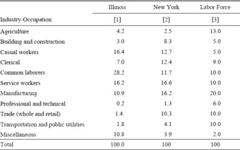
The time frequency of both the national and regional datasets is a month. “City” represents a city in which the PEOs were located. “Industry-occupation group” is a classification used by state PEOs and is similar to the one-digit standard industrial classification code, shown in Table 1. National data was collected from “A Monthly Report of Activities of State and Municipal Employment Services Cooperating with United States Employment Services” published by the U.S. Employment Service (January 1924–January 1932); Illinois state data was obtained from “The Labor Bulletin,” published by the State of Illinois Department of Labor (1922–1933); and New York state data was obtained from “The Industrial Bulletin,” published by the State of New York Industrial Commission (1924–1933).
INDUSTRY-OCCUPATION DISTRIBUTION OF JOB SEEKERS IN PUBLIC EMPLOYMENT OFFICES (PEOS) AND WORKERS IN THE LABOR FORCE

Note:
The unit is percentage. For Illinois the distribution was constructed using the data from 1922 to 1932. For New York it was constructed using the data from 1924 to 1933. For the labor force it is the average of Census data between 1920 and 1930.
For the national and Illinois state data, “Registrations” was used for the number of job seekers; “Help Wanted” was used for the number of job vacancies; and “Placed” was used for the number of new matches. For New York state, “Workers Seeking Employment” was used for a proxy for the number of job seekers; “Workers Called for by Employers” was used for the number of job vacancies; and “Places Reported Filed” was used for the number of new matches. Registrations and Workers Seeking Employment represented the sum of the number of new applicants who were looking for a job and also for renewals at a PEO in a month. When the same job seeker renewed his or her registration in a year, it was not regarded as a new registration (Stewart and Stewart Reference Stewart and Stewart1933, pp. 61–62). Help Wanted and Workers Seeking Employers represented the total number of workers requested by prospective employers to PEOs in a month. Placed and Places Reported Filed were the number of applicants who were hired when referred to employers, with PEOs requiring evidence of engagement before recording a placement (Stewart and Stewart Reference Stewart and Stewart1933, p. 69–70).
Registrations, Help Wanted, and Placed in the historical records fit the main variables of the matching-function framework. In current literature, a number of researchers have used the data from PEOs to estimate matching functions (e.g., Boeri and Burda Reference Boeri and Burda1996, for Czech Republic; Coles and Smith Reference Coles and Smith1996, for Britain; Berman Reference Berman1997; Yashiv Reference Yashiv2000, for Israel; Kano and Ohta Reference Kano and Ohta2005, for Japan).
Although the PEOs played an important role in the employment service in the early twentieth century, it is not certain whether the PEO's national data was fully representative of the entire labor market, because no general evidence has been found.Footnote 11 Alternatively, there are other sources shown in Table 1, which lists the industry-occupation groups classified by the Illinois and New York state PEOs. Columns [1] and [2] display the two states' industry-occupation distribution of PEO users for the 1920s and early 1930s. Column [3] presents the distribution of workers in the labor force. It was constructed by the author, using the information found in the Census (U.S. Census Bureau 1975). Estimates for the labor force might not be perfect because the Census provided the data either by industry or by occupation, but the classification of PEOs in the early twentieth century was a mix of these two items. Since the U.S. Census Bureau provided decennial information for this period, the distribution was measured as an average in the 1920 and 1930 Censuses. The distribution was constructed by using the information found in “Labor Force and Employment, by Industry” and “Detailed Occupation of the Economically Active Population” in the Census. For example, in terms of industry categorization, the data shows that more than 20 percent of the total labor force was employed in agriculture during this period, but the estimated share for agriculture in Table 1 is only 13 percent. This number was calculated by subtracting the number of farm laborers from the number of workers in the agricultural sector. Thus, after the subtraction, the number of agricultural workers represents the sum of farmers (owners and tenants), farm managers, and farm foremen. Farm laborers become a part of “common laborers” in Table 1.
Table 1 shows that all types of workers used PEOs in Illinois and New York states, but most clients were relatively low-skilled workers, such as casual workers, common laborers, and service workers. Thus, the data from the PEOs is not fully representative of the labor force but explains only a sub-sample of the labor market, i.e., the public labor exchange. In general, the majority of workers who sought jobs, through PEOs in the early twentieth century, were unskilled workers, immigrants, or interstate migrants (Rosenbloom Reference Rosenbloom2002, p. 75; Lee Reference Lee and Autor2009, pp. 166–68). However, some proportion of workers in this period, who were classified as semi-skilled or skilled, were actually unskilled. This implies that the actual proportion of unskilled workers was likely to have been higher than that enumerated in the Census (Goldin Reference Goldin, Engerman and Gallman2000). Moreover, the dataset is better suited for the 1930s because the majority of unemployed workers, during the Great Depression, were low skilled (Margo Reference Margo1993). Therefore, the data from the PEOs, in this period, is more representative of the population of interest and may have more information on the unemployed than the Census.
STATE OF LABOR THE MARKET IN THE 1920S AND EARLY 1930S
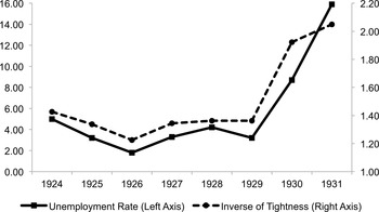
This section presents the state of the labor market during the 1920s and the early stage of the Great Depression with the use of key indices related to the job-matching process. Figure 1 compares the unemployment rate and the inverse of the labor-market tightness (tightness, hereafter) between 1924 and 1931. Tightness is a measure of excess or relative labor demand and is defined as the ratio of the number of job vacancies to the number of job seekers. As tightness becomes higher, a job seeker is likely to have higher probability of finding a job, and thus unemployment tends to be lower, whereas an employer needs to make more effort or must wait longer to fill a vacant job.
UNEMPLOYMENT RATE AND THE INVERSE OF LABOR-MARKET TIGHTNESS

Figure 1 shows that the unemployment rate and the inverse of tightness were both stable in the 1920s. It also shows that both measures soared in 1930 and 1931, which indicates that there was a deterioration of the labor market in the initial stage of the Great Depression. As the number of job seekers increased, the unemployment rate increased, as did the inverse of tightness (the correlation is approximately 0.94). Thus, tightness captures the cyclical behavior of the labor market. Furthermore, tightness is more advantageous because the numbers of job seekers and vacancies were collected monthly, while the unemployment rate was only available on an annual basis. Hence, a closer examination of the state of the labor market in the 1920s and the early 1930s is possible by utilizing the monthly data.
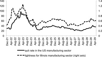
Another advantage of using tightness is a strong positive relationship with the quit rate. The existence of a tighter labor market indicates more job openings, and thus higher voluntary quits of workers for a better job. Figure 2 shows that there was a close movement of the U.S. manufacturing sector's quit rate and the Illinois manufacturing sector's tightness in the 1920s. The correlation between these two indicators was calculated as 0.86, and a one-month lag of tightness was used, it became stronger, and increased to 0.90. Here, using a one-month lag incorporates the lapse of time between a worker's decision to quit and the resulting changes in labor demand.Footnote 12 A strong association between tightness and the quit rate also supports the argument that a substantial decline in the quit rate, in the 1920s, was the result of slack labor markets (Jacoby Reference Jacoby1985).
LABOR-MARKET TIGHTNESS AND QUIT RATE IN THE MANUFACTURING SECTOR

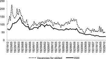
Figure 3 displays the trends in job vacancies for skilled workers in the Illinois PEOs and the Help Wanted Advertising Index (HWI). The skilled workers included “professional-technical,” “clerical,” and, “manufacturing” workers because the HWI was biased toward professionals, white-collar, and skilled workers (Boschan Reference Boschan1966, p. 501). The HWI was an indicator of labor demand, which closely followed the pattern of the U.S. business cycle during the early twentieth century (Boschan Reference Boschan1966, p. 502).Footnote 13 It is shown that skilled workers' vacancies and the HWI shared a similar pattern: the correlation was 0.86. Hence, although it was not fully representative, the data from the PEOs is still useful in examining the labor market for the early twentieth century.
HELP WANTED ADVERTISING INDEX (HWI) AND VACANCIES FOR SKILLED WORKERS

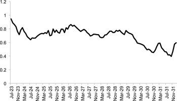
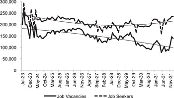
Figure 4 presents tightness, using the nationwide data of the PEOs from July 1923 to January 1932. In the 1920s, tightness was less than one, indicating that there were more job seekers than vacant jobs in the public labor exchange. In Figure 4, the key point is that a considerable drop in tightness during the early 1930s indicates more unfavorable labor market conditions during the early stage of the Great Depression. Figure 5 shows that the number of job seekers was higher than that of job vacancies in the 1920s and this gap became substantial with the onset of the Great Depression, mainly due to a decline in job vacancies. Hence, it is shown that a sharp reduction in tightness in Figure 4, during the Depression, was mainly driven by a substantial drop in the number of job vacancies.
LABOR-MARKET TIGHTNESS AT THE NATIONAL LEVEL

TRENDS OF JOB SEEKERS AND JOB VACANCIES FOR THE NATION

The tightness is a well-established measure in examining the state of the labor market, yet it has a drawback. Since the values of tightness are relative, there is no single reference point to identify the balance of the labor market. For example, William Beveridge (Reference Beveridge1945), who first utilized the concepts of unemployment and job vacancies, defined the state of full employment in which the number of vacancies slightly exceeds the number of unemployed workers (as cited in Bleakey and Fuhrer 1997, p. 3). Moreover, it is still not obvious how slack labor demand affected the job-matching process to create new hires. In the following sections, matching functions will be used to explore this issue.
OVERVIEW OF THE MATCHING FUNCTION
Friction in the job-matching process can explain why unemployment and vacant jobs coexist. The matching function is a simple way to model the kinds of friction that causes transaction costs in the labor market and it has been widely used in macroeconomic literature (Petrongolo and Pissarides Reference Petrongolo and Pissarides2001, p. 390; Pissarides Reference Pissarides2000, p. 6; Cahuc and Zylberberg Reference Cahuc and Zylberberg2004, p. 504). The matching function identifies the number of new matches (M) in a given interval on the basis of the quantity of job seekers (S) and job vacancies (V). In the matching-function framework, the joint movement of job seekers and vacancies, together with the following properties, describes the matching process:


Equation (1) is a general form of the matching function. Equation (2) implies that the matches increase when the number of job seekers and/or job vacancies increases. Equation (3) shows that no hire can be made without at least one job seeker and one vacant job. The matching function is assumed to be concave by Equations (2) and (4).
Two more assumptions are generally introduced to formulate the matching function. The first assumption is that S equals the number of unemployed (Cahuc and Zylberberg Reference Cahuc and Zylberberg2004, p. 521). Second, constant returns to scale are assumed for theoretical convenience (Pissarides Reference Pissarides2000).
The number of job seekers collected from the PEOs in the estimation includes all job seekers, on-the-job searches and unemployed workers, which is advantageous because the actual friction in the labor market is caused by the interactions among all job seekers. Most job seekers who used PEOs in the early twentieth century were unemployed, and hence the assumption that only the unemployed were counted as job seekers can be preserved (Stewart and Stewart Reference Stewart and Stewart1933, p. 229).
This study mainly uses a Cobb-Douglas representation of the matching function in Equation (5) as it is the most widely used functional form in the literature (Pissarides Reference Pissarides2000, p. 2).Footnote 14

where

Here, i represents a cross-sectional unit (city, state, or industry-occupation group) and t is time (month). All the variables are indexed by i and t because a panel data structure is used in this article. By taking the natural logarithm of both sides, a Cobb-Douglas specification of the matching function is

γ i is the occupation or the region-specific fixed effects and T represents the time trend or time dummies.Footnote 15 γ and δ can often be interpreted as additional effects in the efficiency of the matching process across occupations, regions or over time. α is interpreted as the elasticity of the matching function with respect to job seekers and β is the elasticity with respect to job vacancies. The degree of returns to scale for the matching technology is easily obtained by the sum of α and β and can be tested under the null hypothesis of constant returns to scale: α + β = 1 in (5) or (6).
Estimates of the matching function deliver the relevant information in terms of a policy perspective. The elasticities of matches with respect to job seekers and vacancies, α and β, respectively, are interpreted as the absolute and relative importance of supply and demand in creating new hires or in the contributions of job seekers and vacancies in the job-matching process. In a labor market characterized by a small α, but large β, or exhibits a relative deficiency in labor demand, an additional vacancy leads to a new match with a high probability, while an additional job seeker creates virtually no new hires (Fahr and Sunde Reference Fahr and Sunde2004, p. 411). In this situation, policies to stimulate demand rather than supply would be suitable for new job creation.Footnote 16
Dynamic panel regressions are performed because the time frequency, t, is measured in terms of length of time. In the matching function for the nation, the data span from January 1924 to January 1932, or over a total period of 97 months. In this case, the lagged effects of both the dependent and control variables can cause the estimates to be biased (e.g., Phillips and Moon Reference Phillips and Moon2000). In the Cobb-Douglas case, a specification of the dynamic panel regressions is:

where c(L) = φ 1 L + φ 2 L 2 + … + φp L p ;d(L)= α 1 L + α 2 L 2+ … + α q L q ; f(L)= β 1 L + β 2 L 2+ … + β r L r . L is the lag operator. The potential lagged effects can be controlled by adding the lagged values of the dependent variable and the covariates.
Research in empirical matching functions follows two approaches: an economy-wide aggregate matching function (e.g., Pissarides Reference Pissarides1986, for the United Kingdom; van Ours 1991, for the Netherlands; Fêve and Langot 1996, for France; Mumford and Smith Reference Mumford and Smith1999, for Australia; and Yashiv Reference Yashiv2000, for Israel) and a disaggregated matching function across regions or industries (e.g., Anderson and Burgess 2000, for the four U.S. states of Georgia, Louisiana, Missouri, and South Carolina; Burgess and Profit 2001, for the United Kingdom; Burda and Profit Reference Burda and Profit1996, for the Czech Republic; and Kano and Ohta Reference Kano and Ohta2005, for Japan).
Oliver J. Blanchard and Peter A. Diamond (Reference Blanchard, Diamond and Diamond1990), Hoyt Bleakley and Jeffrey C. Fuhrer (Reference Bleakley and Fuhrer1997), and Daniel Borowczyk-Martins, Gregory Jolivet, and Fabine Postel-Vinay (Reference Borowczyk-Martins, Jolivet and Postel-Vinay2013) estimated the economy-wide matching functions for the U.S. labor market. Blanchard and Diamond estimated the economy-wide aggregate matching functions for the 1970s, with elasticities of 0.42 for unemployment and 0.62 for job vacancies, thereby exhibiting constant returns to scale. Bleakley and Fuhrer also estimated the aggregate matching functions for the period 1979 to 1993, with estimates for unemployment and vacancies of 0.64 and 0.36, respectively, and no rejection of constant returns to scale. Under the assumption of constant returns to scale, Borowczyk-Martins, Jolivet, and Postel-Vinay showed that the elasticities of the matching function with respect to job seekers and vacancies between December 2000 and January 2012 were 0.3 and 0.7, respectively.
The degree of returns to scale is one of the main issues in literature on matching function. The constant returns to scale, for the matching function, are assumed to generate a stable and unique unemployment rate in the search-matching models of equilibrium unemployment (e.g., Pissarides Reference Pissarides2000). In addition, constant returns mean that the matching rate for job seekers (M/S) depends only on tightness (V/S), meaning that the actual size of the market for (i.e., the number of) job seekers or vacancies does not affect the creation of new hires, but the relative size does. The decreasing returns to scale of the matching function imply a congestion effect in the matching process, with more friction existing in larger labor markets. Put differently, the matching efficiency decreases as the volumes of job seekers and vacancies increase. The presence of increasing returns to scale implies either high or low activity in terms of unemployment equilibrium due to the existence of strong positive externalities (Petrongolo and Pissarides Reference Petrongolo and Pissarides2001, p. 393). In one situation, employers and job seekers put more effort into their searches. In the other situation, both agents put less effort into their searches and experience lower returns, this latter scenario causes a lower matching rate and, thus higher unemployment.Footnote 17 Overall, although there are some exceptions, most empirical studies have accepted the hypothesis of constant returns to scale, especially with aggregate or macroeconomic data (Petrongolo and Pissarides Reference Petrongolo and Pissarides2001, p. 397).
EMPIRICAL MATCHING FUNCTIONS: 1924–1932
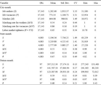
Table 2 provides the descriptive statistics for the variables used in the matching-function estimation for the period from January 1924 to January 1932. It also presents matching rate for workers, matching rate for vacancies, and V-S ratio for examining the process of matching. The average number of job seekers in a city, in a month, was more than 1,200, while the average number of job vacancies and matches were 771 and 664, respectively. The averages of these three variables signify a lack of labor demand in the job matching process before controlling for heterogeneities across cities. A higher average matching rate for vacancies than for job seekers and a low average of tightness support the vacancy-reliant matching process. The high standard deviations of job seekers, vacancies, and matches reveal considerable variations across regions and time. But the coefficient of variation shows that there was almost no difference in the degree of variations between these variables for this period. Variations in the matching rate for job seekers, the matching rate for vacancies, and tightness were much smaller than the numbers of job seekers, vacancies, and matches. These patterns did not change at the state-month level. The degrees of variation for all six variables become much smaller at the nation-month level.
DESCRIPTIVE STATISTICS (1924:1–1932:1)

Note:
CV stands for the coefficient of the variation, which is the ratio of the standard deviation to the mean and is used as a measure of dispersion.
Sources:
See the text.
In estimation, the Cobb-Douglas, tanslog, and constant elasticity of substitution (CES) specifications were employed. Panel regressions were performed for the Cobb-Douglas and translog, and a nonlinear least squares estimation was utilized for the CES model. The results reported are the outcomes only for the Cobb-Douglas specification by the panel regression with fixed effects: the parameter estimates in the Cobb-Douglas and translog models did not produce different interpretations; the functional form test in the CES regression suggests the Cobb-Douglas; there was no difference in the estimates between the fixed-effects and first-differencing methods; no difference was detected between the fixed-effects and random-effects models; and fixed-effects were preferred to random-effects in the Hausman test.Footnote 18 , Footnote 19 For each variable, panel-based unit root tests were performed and the hypothesis of non-stationarity was rejected in all cases.Footnote 20 I added month dummies to all specifications of the matching function to deal with seasonal effects. Also I used time-fixed effects, instead of time trends, to capture business-cycle effects. But only the results obtained using time trends were reported because there was no difference in the estimated coefficients.Footnote 21 The standard errors reported in all tables were heteroscedastic robust standard errors.Footnote 22
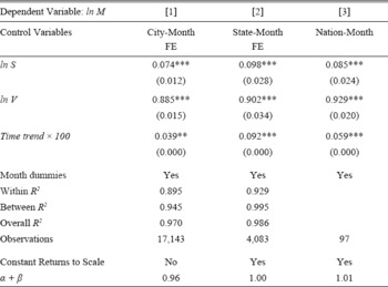
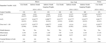
Column [1] in Table 3 presents the main results from estimating the matching function. The positive and significant estimates for job seekers and vacant jobs were consistent with the theories of the search and matching. The main implication is that there was a substantial deficiency of labor demand in the national labor market during the 1920s and the early 1930s. The elasticity with respect to job seekers was very low, 0.07, while the elasticity with respect to job vacancies was 0.89. This indicates that job vacancies had the most weight in the creation of job matches and the contribution of job seekers was minimal during this period. The addition of city fixed effects, time trend, and a strong co-movement between job seekers and vacancies may result in a high R-squared value.Footnote 23
EMPIRICAL MATCHING FUNCTIONS FOR THE NATION: MAIN RESULTS (1924:1–1932:1)

* = Significant at the 10 percent level.
** = Significant at the 5 percent level.
*** = Significant at the 1 percent level.
Notes:
[1] and [2] are the results from the panel regressions with fixed effects (the case unit is a city for [1] and a state for [2]). [3] is the result from Newey-West standard errors. Prais-Winsten and Cochrane-Orcutt regressions (feasible GLS methods) were also performed to deal with autocorrelation and the difference is trivial between the Newey-West and the feasible GLS methods. Column [1] shows the main results of estimating the disaggregated matching function at the city-month level and columns [2] and [3] are the results used to examine the spatial aggregation problem. For the test of constant returns to scale, H0: α + β = 1 and the 5-percent level of significance is used for the F test.
Sources:
See the text.
The spatial aggregation problem, a frequently raised problem in the estimation of matching functions (e.g., Coles and Smith Reference Coles and Smith1996) was investigated, and Table 3 displays the results. As the data is aggregated from city to state and then to the national level (columns [1], [2], and [3]), the degree of returns to scale changes from decreasing to constant returns to scale, meaning that the spatial aggregation bias could affect the empirical results, especially the degree of returns to scale. In practice, the results show that the spatial aggregation bias was not important for the matching function in the 1920s and early 1930s. It is because the estimates for the matching parameters were not qualitatively different in all cases and the matching function tended to exhibit constant returns to scale, at least qualitatively (α + β is approximately one through columns [1], [2], and [3]).
Another way of defining the labor market is to assume that it is a collection of industries or occupations. Similar to Patricia M. Anderson and Simon M. Burgess (Reference Anderson and Burgess2000), industry-occupation groups were used as cross-sectional variations in the matching functions for Illinois and New York states.Footnote 24 The classification of these groups is listed in Table 1. The regional labor markets are defined as a collection of industry-occupation groups, which capture differences in skill requirements and job characteristics, and other heterogeneities in the job-matching process. Table 4 indicates that there was no significant difference between the estimates of the city-level data and those of the industry-occupation level, which are shown by the estimates for ln(S) and ln(V). In all cases, the estimates for job seekers were very small and those for job vacancies were considerably large. This indicates that defining the labor market as a collection of regions or industries revealed the same implications for this period. The degree of returns to scale was also close to unity in all cases, which implies constant returns to scale of the matching function although the labor market was defined in different ways. The estimates of the matching function and the degree of returns to scale are broadly similar whether one investigates the aggregate economy or cities and states.
EMPIRICAL MATCHING FUNCTIONS FOR THE NATION, ILLINOIS, AND NEW YORK: INDUSTRY-OCCUPATION AGGREGATION BIAS AND WITH LABOR FORCE DISTRIBUTION

* = Significant at the 10 percent level.
** = Significant at the 5 percent level.
*** = Significant at the 1 percent level.
Notes:
For the test of constant returns to scale (CRS), H0: α + β = 1 and the 5-percent level of significance is used for the F-test. Column [7] is the same as column [1] in Table 3. Columns [3] and [6] are the re-estimated results that were obtained by using the labor force distribution in Table 1. The panel regression was performed with industry-occupation fixed effects and a time trend. The sampling weight = 1 divided by labor force distribution.
Sources:
See the text.
To address the non-representativeness of the data obtained from the PEOs, I re-estimated Illinois and New York states' matching functions across the industry-occupation groups, using the labor force distribution as sampling weights, and the results are shown in columns [3] and [6] in Table 4. Sampling weights were incorporated to correct the data's disproportionality with respect to the population of interest (see, for example, Pfeffermann Reference Pfeffermann1993). In Table 4, column [3] is comparable to column [2], and column [6] to column [5]. The estimates with and without sampling weights were not very distinguishable.Footnote 25 Various sampling weights were incorporated, but the main results were not affected. Since the estimations with and without sampling weights did not produce different implications, using the one without weights was more appropriate because it generated more efficient estimates and the estimated standard errors were correct (Winship and Radbill Reference Winship and Radbill1994).
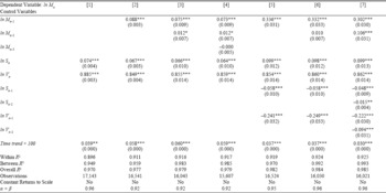
Table 5 reports the results from the dynamic panel regression analysis, specified in Equation (7). All possible dynamics were incorporated, but the elasticities for job seekers and vacancies were not qualitatively different, with and without lags of the independent and control variables.Footnote 26 The estimates for the lagged variables were significant to some degree, implying that past labor market conditions had some impact on the current period's matching process.Footnote 27 Again, however, the key finding is that the matching process was entirely vacancy-dependent.
EMPIRICAL MATCHING FUNCTIONS FOR THE NATION: THE RESULTS FROM DYNAMIC PANEL REGRESSIONS

* = Significant at the 10 percent level.
** = Significant at the 5 percent level.
*** = Significant at the 1 percent level.
Notes:
For the test of constant returns to scale, H0: α + β = 1 and the 5 percent level of significance were used for the F-test.
Sources:
See the text.
Another point of concern is the time-aggregation bias in estimating the matching functions (Petrongolo and Pissarides Reference Petrongolo and Pissarides2001).Footnote 28 However, it is not applicable in this study because all the variables are flow variables, and hence were contemporaneously timed in the matching-function analysis. As the period of validity for job seekers and vacancies was only 15 to 30 days, the quantities that interacted in the matching process through the PEOs were close to the stock values.Footnote 29
THE 1920S VS. THE GREAT DEPRESSION
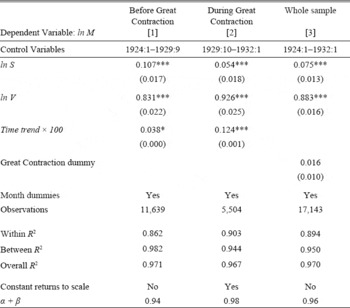
Assuming that the matching technologies were different before and during the Great Depression, I estimated the matching functions, separately for the periods from 1924 to 1929 and the early stage of the Depression, as shown in columns [1] and [2] of Table 6.Footnote 30 The estimate for job seekers was 0.11 and for job vacancies was 0.83 before the Depression, whereas during the Depression, the estimate for job seekers dropped to 0.05, but the estimate for job vacancies rose to 0.93, confirming that the deficiency of job vacancies that prevailed in the public labor exchange in the 1920s worsened in the early stage of the Depression. In other words, the public labor exchange was slack in the 1920s and became slacker as the Great Contraction exerted its full force on the U.S. economy. Also, I estimated a shift in the matching efficiency before and after the Great Contraction and the results are presented in Table 6, column [3]. The estimate for the Great Contraction dummy (October 1929 to January 1932) is even positive, small, and statistically insignificant. This result shows that there was no significant deterioration of the matching efficiency at the early stage of the Great Contraction.
EMPIRICAL MATCHING FUNCTIONS FOR THE NATION (“1920S” VS. “GREAT CONTRACTION”)

* = Significant at the 10 percent level.
** = Significant at the 5 percent level.
*** = Significant at the 1 percent level.
Notes:
For the test of constant returns to scale (CRS), H0: α + β = 1 and the 5-percent level of significance were used for the F-test.
Sources:
See the text.
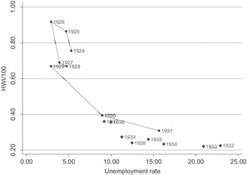
With the use of the other data sources, one of the main findings that there was a slacker labor market and a trivial loss in the matching efficiency at the onset of the Great Depression is observed. Figure 6 displays an empirical Beveridge curve: a plot of the unemployment rate versus the HWI, yearly from 1924 to 1939.Footnote 31 In general, movement along the Beveridge curve toward the bottom-right indicates high unemployment and low vacancies during a recession. An outward shift of the Beveridge curve, from the origin, implies a deterioration of the matching process: more job seekers and vacancies are required to create the same number of new matches. The marked gap between the periods 1924–1929 and 1930–1931, shown in Figure 6, confirms the existence of a slacker labor market during the Great Contraction. The sharp movement from 1929 to 1930 toward the bottom-right along the Beveridge curve displays the magnitude of downturn at the beginning of the Great Contraction. On the graph, the U.S. economy further slides down the Beveridge curve during the Great Contraction from 1932 to 1933, implying further deterioration of the labor market. In comparison with the 1920s, the economy stays in the bottom-right on the Beveridge curve during the 1930s, confirming severe and long-lasting recession in those days. The plots for 1930–1931 do not look far from the origin, compared to the plots for 1924–1929, supporting my finding that there was a trivial change in matching efficiency during the Great Contraction.
BEVERIDGE CURVE IN THE 1920S AND 1930S

SLACK LABOR DEMAND VS. LOW UNEMPLOYMENT RATE IN THE 1920S
The evidence in the previous sections shows that the public labor exchange was slack during the 1920s and became slacker as the Depression hit the economy. A slacker labor market in the 1930s looks reasonable, but the deficiency of job vacancies in the 1920s is not immediately understandable because the unemployment rate was relatively low, approximately 5 percent or less. Therefore, possible explanations for this conflict are discussed.
The most plausible explanation is that major users of the PEOs were casual workers, common laborers, service workers, immigrants, or interstate migrants (Lee Reference Lee and Autor2009). And although the U.S. economy was still booming in the 1920s, these labor groups experienced unfavorable labor market conditions in this period. This can be described by the situation of dual labor markets, “the picture from the 1920s is mixed, depending on who you were and where happened to land a job” (Wright Reference Wright1986, p. 337).
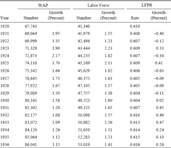
The other possibility is that there were discouraged workers who existed out of the labor force (LF) due to the lack of available jobs. In this case, by excluding discouraged workers, the unemployment rate could have been low despite the slack labor market in the 1920s. The hypothesis of the discouraged worker would be supported by the decline in the labor force participation rate (LFPR) over the decade, as shown in Table 7. Both the working age population (WAP) and the LF steadily grew, but the growth rate of the WAP was greater than that of the LF, which could have generated a larger size non-labor force that included discouraged workers.Footnote 32 Consequently, the size of the LF, the sum of the employed and unemployed, could have been smaller than the actual size due to the absence of discouraged workers in the data. In fact, this phenomenon translates into the lower unemployment rate recorded for the period.
TRENDS OF POPULATION, WAP, LF, AND LFPR, 1920–1936

Notes:
The numerical unit is one thousand. The working age population (WAP) = persons in the total population who are 16 years of age and over. The labor force = the number of employed + the number of unemployed. The labor force participation rate (LFPR) = total labor force / working-age population.
Source:
U.S. Census Bureau (1975).
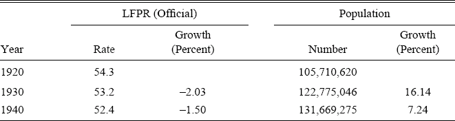
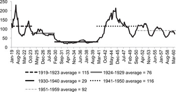
The census data also show a noticeable change in the LFPR. The growth rate of the LFPR between 1920 and 1930 was minus 2.03 percent along with a population growth rate of 16.14 percent (see Table 8). Although the LFPR dropped by 1.5 percent in the 1930s, the reduction was higher in the 1920s. Hence, despite a fairly low unemployment rate and substantial economic growth in the 1920s, it could be inferred that the U.S. labor market would have suffered from slack labor demand. Again, estimates of low unemployment might be explained by the exit of discouraged workers out of the LF due to the scarcity of available jobs. The longer trend of the HWI in Figure 7 also shows that the period 1924 to 1929 experienced a greater deficiency of labor demand than any other period except for the time of the Great Depression. This indicates that it was harder for a job seeker to find a job, i.e., a slack labor market.
LFPR AND POPULATION IN THE CENSUS YEARS, 1920, 1930, AND 1940

Note:
Labor force participation rate (LFPR) and population were taken from the decennial census data.
Source:
U.S. Census Bureau (1975).
TREND OF THE HELP WANTED ADVERTISING INDEX (HWI): JANUARY 1919–AUGUST 1960

ECONOMIC IMPLICATION OF VACANCY-DRIVEN MATCHING FUNCTION
The estimates of the matching function in this article show that the job-creation process was almost entirely vacancy dependent, indicating a lack of labor demand in the public labor exchange during the 1920s and early 1930s. Since the unemployment rate was unusually high and the majority of unemployed workers were low skilled during the Great Depression (Margo Reference Margo1993), it can be inferred that the job-matching process, in general, was vacancy driven, similar to the public labor exchange. In such a case, government policies aimed at stimulating labor demand are suitable for new hires.
Compared to those of the matching parameters for the 1970s and the 1980s, the estimate of the elasticity for job seekers was lower and that of job vacancies was much higher. An interesting point is that, to some degree, the matching process during the period from 1924 to 1931 was similar to that in the 2000s in that both periods' matching functions showed job-vacancy dependence. The estimate for job vacancies in the 2000s was 0.70 (Borowczyk-Martins, Jolivet, and Postel-Vinay Reference Borowczyk-Martins, Jolivet and Postel-Vinay2013). Therefore, valid policy implications for the current situation in the U.S. labor market can be drawn from history.
During the 1930s, the U.S. government introduced a set of policies that offered relief to the unemployed, collectively known as the New Deal. Among these policies, an injection of new jobs, such as those created by the Civil Works Administrations (CWA), seemed to be a relevant response to a lack of labor demand. The CWA hired more than 4 million people in the winter of 1933–1934, and most of the placements were made by the PEOs (Atkinson, Odencrantz, and Deming 1938, pp. 28–30). However, some active labor market policies that were aimed at stimulating labor supply might not have been suitable for the slack labor market that existed during this period. For example, the National Relations Act (the Wagner Act) in 1935 was designed to assist labor unions in raising workers' wages, which boosted labor supply. This type of policy might not have been effective in the face of the deficiency of labor demand during the Great Depression.
CONCLUDING REMARKS
This article presents a detailed empirical analysis of the matching between job seekers and vacancies, during the 1920s and the early stage of the Great Depression. The investigation was based on estimations of the matching functions at the city-month level, using data extracted from public employment offices. This study is the first in-depth work to estimate the matching functions for the U.S. labor market during this period. Although the data from public employment offices are closely related to other indicators that represent the state of the labor market that existed in the early twentieth century, the results should be interpreted with caution because the data are not fully representative of the labor market as a whole.
On the basis of the results of the matching functions and the historical data, this article proposes a hypothesis for a conflict between the low unemployment rate and the deficiency of labor demand that existed in the 1920s. Although the most plausible story is that the slack labor demand only pertained to the public labor exchange, there is a possibility of the “discouraged-worker effect” having an impact during this period. Regardless of the outcome of this study, the shrinkage of the labor force participation rate in the 1920s, caused by the higher growth rate of that working age population compared to that of the labor force, may had led to a larger size non-labor force that included discouraged workers.
Using the results that showed a lack of labor demand, especially for the 1930s, I evaluated the relevance of some active labor market policies, such as the Civil Works Administration and the Wagner Act, which may also be a valuable contribution to the literature. However, for a more rigorous policy assessment, the estimates of the matching-function parameters should be incorporated and analyzed in the search-matching model. Lastly, a detailed research is proposed that compares the states of the labor market between the periods of the Great Depression of the 1930s and the Great Recession of the 2000s. It is interesting to note that, in contrast to the situation of an outward shift in the Beveridge curve, since the second half of 2009 (Diamond and Şahin Reference Diamond and Şahin2014), it is shown that the Beveridge curve shifted inward as the U.S. economy recovered during the 1930s.