1 Introduction
Among the large variety of materials fashioned for industrial needs, super-hydrophobic (SH) surfaces have attracted an increasing attention since the 1990s (Quéré Reference Quéré2008). Resulting from the combination of surface texturing and chemical repellency (Shirtcliffe et al. Reference Shirtcliffe, McHale, Atherton and Newton2010), SH surfaces in the so-called Cassie–Baxter state (Cassie & Baxter Reference Cassie and Baxter1944) can entrap a gas layer, referred to as the plastron, in their roughness, thereby restricting the solid/liquid contact area. This feature yields slippage, which may have a strong impact in a wide range of engineering applications where wettability control is essential (Zhang et al. Reference Zhang, Xia, Kim and Sun2012). In the framework of drag control, a number of studies have evidenced the beneficial effects of SH surfaces in reducing skin friction at laboratory scale (Rothstein Reference Rothstein2010). However, the extrapolation of these results under broader operating conditions is still to be demonstrated (Samaha, Tafreshi & Gad-el-Hak Reference Samaha, Tafreshi and Gad-el-Hak2012). One of the main arising issues is the stability of the gas/liquid interface leading eventually to plastron failure (the so-called transition from the Cassie–Baxter state to the Wenzel state), which is a cornerstone to warrant the effectiveness and the sustainability of SH surfaces (Piao & Park Reference Piao and Park2015). In particular, the effects of flow-induced perturbations on the interface stability and the possible feedback of plastron compliance on the flow still represent a tough challenge for current theoretical studies and numerical simulations.
The range of scales featuring the problem is so huge that a full resolution is unrealistic. Furthermore, solving a two-phase flow involving stiff jumps of density at the gas/liquid interface is a challenging issue. To bypass these constraints, the interface between the gas and the liquid can be modelled by a non-deformable surface, thereby neglecting the effect of surface tension. For instance, the slip-length model is a popular boundary condition used in a large number of numerical simulations or theoretical studies to mimic SH surfaces from partial slip (see e.g. Min & Kim Reference Min and Kim2004; Ybert et al.
Reference Ybert, Barentin, Cottin-Bizonne, Joseph and Bocquet2007) to perfect slip (see e.g. Lauga & Stone Reference Lauga and Stone2003; Martell, Blair Perot & Rothstein Reference Martell, Blair Perot and Rothstein2009). In this approach, the liquid phase flows over patches of slip/no-slip areas arranged either regularly or randomly. Recently, more realistic approaches have been deployed by simulating the flows within the two phases (Gruncell, Sandham & McHale Reference Gruncell, Sandham and McHale2013; Jung, Choi & Kim Reference Jung, Choi and Kim2016) but still avoiding any deformation of the gas/liquid interface. Neglecting the plastron compliance relates to two major assumptions: (i) there is no possible feedback on the flow due to the shape modification of the boundary condition and (ii) the plastron is presumed resilient even for high-speed flows. The relevance of these assumptions is disputed by experimental observations at both low and high Reynolds numbers. Byun et al. (Reference Byun, Kim, Ko and Park2008) investigated the flow within microchannels with transverse grooves. They observed curved gas/liquid interfaces, which induced wavy flow on the grooves for large pitch-to-width ratios. In some cases, plastron depletion was reported. Kim & Rothstein (Reference Kim and Rothstein2017) studied the influence of the gas/liquid interface on the laminar flow over an array of SH pillars spanning the entire height of a microchannel. Both pressure and viscous drag were found to be sensitive to the curvature of the air bubbles entrapped within the pillar cavity. Studying respectively turbulent flows over a flat plate and circular cylinders treated with SH coatings, Aljallis et al. (Reference Aljallis, Sarshar, Datla, Sikka, Jones and Choi2013) and Kim, Kim & Park (Reference Kim, Kim and Park2015) reported performance losses once the air plastron was washed out. This issue has been addressed recently in studies aiming at identifying the limits at which plastron failure is likely to occur. Piao & Park (Reference Piao and Park2015) investigated theoretically the longevity of the plastron in a single two-dimensional (2-D) groove subjected to harmonic pressure fluctuations and gas diffusivity. They found that for underwater applications where the immersion depth is typically
 $O(\text{m})$
, the pressure-induced perturbation is the leading-order effect. Their findings revealed that the interface stays stable only for small enough widths of the groove, i.e.
 $O(\unicode[STIX]{x03BC}\text{m})$
. Based on the direct numerical simulations (DNS) of a turbulent channel flow, Seo, García-Mayoral & Mani (Reference Seo, García-Mayoral and Mani2015) investigated the pressure induced by the footprint of the surface texture modelled as a local shear-free condition. The resulting averaged pressure distribution was then used to predict the typical interface deformation over a groove. Although their approach was restricted to an one-way coupling, these authors delineated critical texture size beyond which plastron failure may occur, which was found to depend on both the pattern width and the Weber number expressed in wall units.
This has motivated us to investigate the possible interplay between the flow and the gas/liquid interface, which is at the core of this study. To this end, we designed an experimental set-up to study the hydrodynamic performance of free falling SH spheres, which have been chosen as a prototype geometry. A large number of experimental, numerical and theoretical works have been devoted to the investigation of the wake of free falling/rising bluff bodies (see Ern et al. Reference Ern, Risso, Fabre and Magnaudet2012, and references therein). All in all, these studies emphasised the key role of the vorticity generated at the surface of the bodies in the development of the wake (see e.g. Leal Reference Leal1989; Magnaudet & Mougin Reference Magnaudet and Mougin2007; Auguste & Magnaudet Reference Auguste and Magnaudet2018). Indeed, the amount of vorticity produced within the boundary layer developing on the surface of the body is at the root of the onset of wake instabilities and has a direct impact on the hydrodynamic forces (Wu, Lu & Zhuang Reference Wu, Lu and Zhuang2007). In addition to parameters such as Reynolds number or buoyancy effect, several works pointed out the sizeable influence of both body shape and slip condition at the body surface on the production of vorticity. For freely rising elongated bodies, Fernandes et al. (Reference Fernandes, Risso, Ern and Magnaudet2007) investigated the critical Reynolds number at which the onset of wake instabilities appears, with respect to the aspect ratio. They reported lower critical Reynolds numbers than those of spheres. Earlier transition was also observed by Jenny, Dušek & Bouchet (Reference Jenny, Dušek and Bouchet2004) for imperfect spheres produced either by damaging the surface or by displacing the centre of gravity. Using 2-D DNS at low Reynolds number, Legendre, Lauga & Magnaudet (Reference Legendre, Lauga and Magnaudet2009) investigated the effect of slip boundary condition on the production of vorticity at the surface of a circular cylinder. They showed that the slip condition delays the appearance of wake instabilities and yields drag and lift mitigation. Based on a two-phase approach, Gruncell et al. (Reference Gruncell, Sandham and McHale2013) simulated the steady laminar flow around a sphere encapsulated within an air layer. A significant drag reduction was obtained with respect to the dimensionless plastron thickness. The influence of the shape of bodies with perfect slip was studied by Mougin & Magnaudet (Reference Mougin and Magnaudet2002a ) and Magnaudet & Mougin (Reference Magnaudet and Mougin2007) who carried out DNS of flows around non-deformable oblate spheroidal bubbles. They evidenced that the maximum surface vorticity increases with the aspect ratio of the bubble. Exploring a wide range of control parameters, they observed that wake instabilities appear for high enough aspect ratio and coincide with the increase of flow-induced loads.
Very few experimental works have been dedicated to the study of the drag of spheres covered by an SH coating. McHale et al. (Reference McHale, Shirtcliffe, Evans and Newton2009) performed falling experiments of SH acrylic spheres over a wide range of terminal Reynolds number
 $Re_{\infty }$
(based on the diameter of the sphere and its falling terminal velocity) using several surface treatments. An intermediate sand layer was deposited to vary the surface roughness. The authors investigated the change in terminal velocity and accordingly in drag with and without the presence of the air plastron. More recently, another falling sphere experiment was carried out by Ahmmed, Patience & Kietzig (Reference Ahmmed, Patience and Kietzig2016) using laser-textured polytetrafluoroethylene (PTFE) spheres at both low and high
 $Re_{\infty }$
using glycerine/water mixtures. Although the ranges of
 $Re_{\infty }$
investigated by McHale et al. (Reference McHale, Shirtcliffe, Evans and Newton2009) and Ahmmed et al. (Reference Ahmmed, Patience and Kietzig2016) do not overlap, some data were collected at comparable
 $Re_{\infty }$
. Within the Cassie–Baxter state, significant drag reduction (
 ${\approx}$
10 %) was achieved by McHale et al. (Reference McHale, Shirtcliffe, Evans and Newton2009) for
 $Re_{\infty }\approx 10^{4}$
. On the contrary, at
 $Re_{\infty }\approx 5\times 10^{3}$
, Ahmmed et al. (Reference Ahmmed, Patience and Kietzig2016) evidenced a decrease of the terminal velocity by up to 10 % yielding an increase by 20 % of the drag in comparison to standard spheres. These somehow discordant results illustrate that a comprehensive understanding of the flows over SH bluff bodies is still missing.
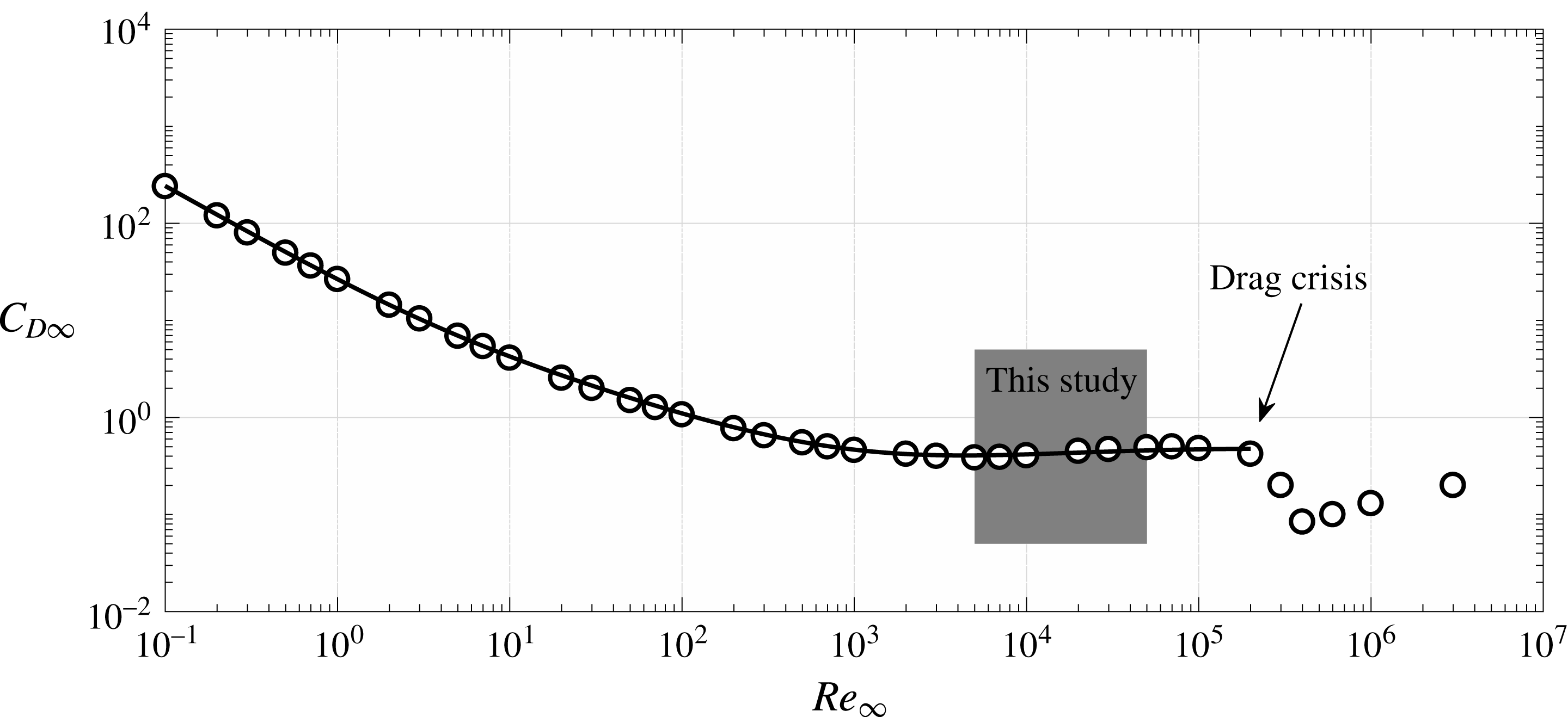
Drag coefficient as a function of the Reynolds number for smooth spheres. ○, Experimental data (Lapple & Sheperd Reference Lapple and Sheperd1940). Solid line: semi-empirical law (Cheng Reference Cheng2009) valid up to
 $Re_{\infty }=2\times 10^{5}$
. The present study focuses on the sub-critical regime, before the appearance of the drag crisis phenomenon.

This study aims at providing new insights about the physical mechanisms governing the development of the wake of SH spheres. To the best of our knowledge, no attempt has yet been undertaken to study the influence of the plastron compliance. This is the main goal of this work. The motivation of this study is twofold: (i) evidencing and characterising the interface distortion and (ii) investigating the feedback of the plastron deformation onto the wake of the sphere. To this end, particular attention is given to the onset of the wake instabilities and the hydrodynamic loads experienced by the SH spheres. In order to highlight the role of the plastron deformation, the dependency of the flow on other parameters must be as small as possible. In particular, the flow regime must be chosen to be Reynolds independent. The well-known evolution of the terminal drag coefficient
 $C_{D\infty }$
of a sphere is plotted in figure 1 with respect to
 $Re_{\infty }$
(Lapple & Sheperd Reference Lapple and Sheperd1940). Large variations of Reynolds number imply modification of the involved phenomena and of the flow-induced stresses on the plastron. The low
 $Re_{\infty }$
region was partially investigated (
 $Re_{\infty }=2\times 10^{-1}$
and
 $Re_{\infty }=2\times 10^{3}$
) by Ahmmed et al. (Reference Ahmmed, Patience and Kietzig2016), who found no drag reduction with respect to standard spheres, in agreement with their results at
 $Re_{\infty }\approx 5\times 10^{3}$
. In the larger
 $Re_{\infty }$
region dominated by the drag crisis phenomenon, falling sphere experiments were also performed by considering an air plastron sustained by the Leidenfrost effect (Vakarelski et al.
Reference Vakarelski, Marston, Chan and Thoroddsen2011), a super-hydrophobic coating (Jetly, Vakarelski & Thoroddsen Reference Jetly, Vakarelski and Thoroddsen2018) or a combination of both (Vakarelski et al.
Reference Vakarelski, Patankar, Marston, Chan and Thoroddsen2012; Vakarelski, Chan & Thoroddsen Reference Vakarelski, Chan and Thoroddsen2014). These studies evidenced drag reduction up to approximately
 $80\,\%$
due to an early drag crisis transition with respect to reference spheres. The air layer appeared to be able to promote the movement of the separation point of the turbulent boundary layer towards the rear side of the falling sphere, causing a narrowing of the wake. Within this study, the focus is put on the so-called sub-critical regime, which is featured by the massive separation of the laminar boundary layer (Achenbach Reference Achenbach1972). As illustrated in figure 1, the drag coefficient characterising this regime is approximately constant, which means that the flow is weakly dependent on Reynolds number.
The paper is organised as follows: the experimental set-up and the manufacturing procedure of the SH coatings are described in § 2. The deformation of the plastron is investigated in § 3, while its influence on the hydrodynamic performance of the falling spheres is discussed in § 4.
2 Experimental set-up and manufacturing procedure
2.1 The falling sphere experiment
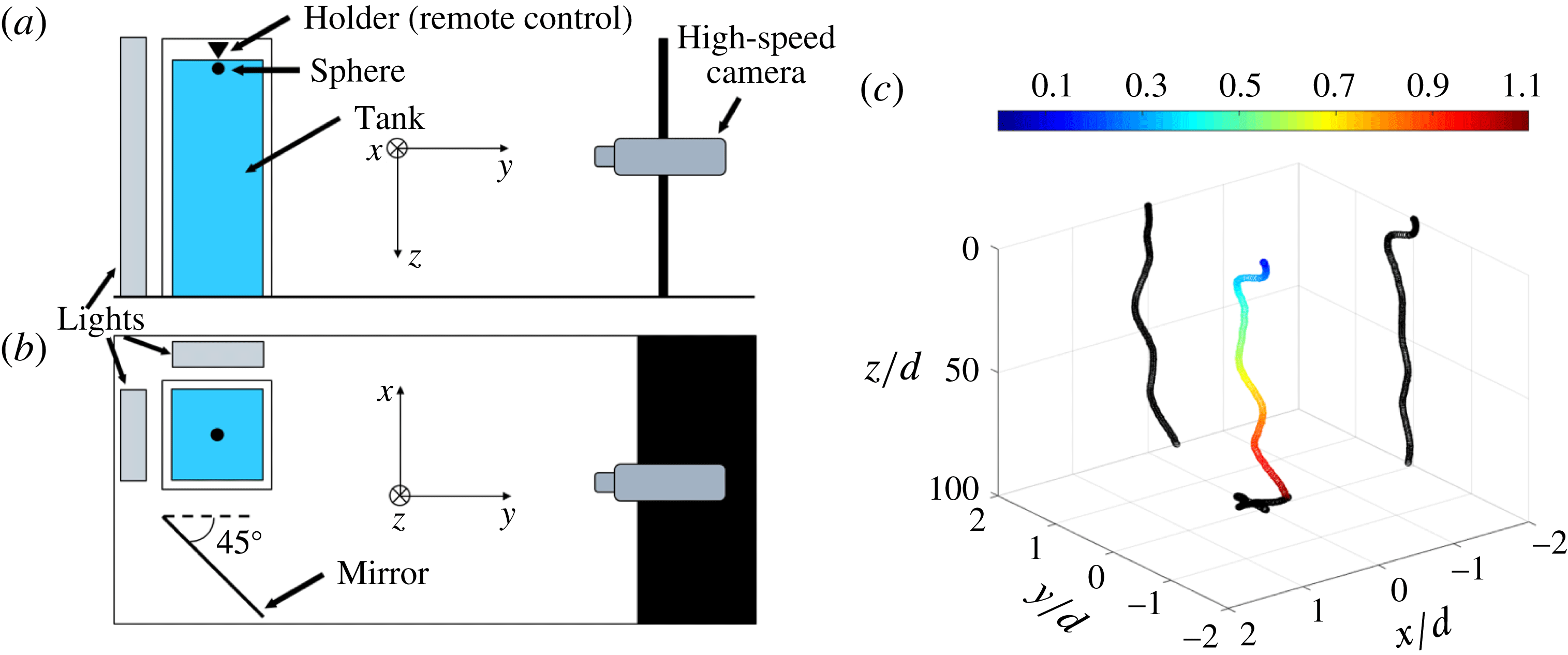
The experiments were performed in a transparent tank (
 $100\times 100~\text{mm}^{2}$
cross-section and 650 mm height) filled with double-distilled water (see figure 2
a,b). In this study, stainless steel bearing spheres with nominal diameter
 $d$
ranging from 5 to 25 mm were used as reference. Before each try, the spheres were gently dipped beneath the water surface by means of an electromagnetic holder, which was used to accurately control their release. Blank tests were performed in order to exclude significant effects of the electromagnetic field on the sphere drops. During the tests the temperature of the water was monitored by a thermocouple and was kept around
 $19\,^{\circ }\text{C}$
.
The falling sphere experimental set-up: (a) side view and (b) top view. (c) Typical example of a three-dimensional trajectory of a free falling sphere. The colour scale indicates the sphere velocity in
 $\text{m}~\text{s}^{-1}$
. The black curves represent the projections of the trajectory on the three planes.
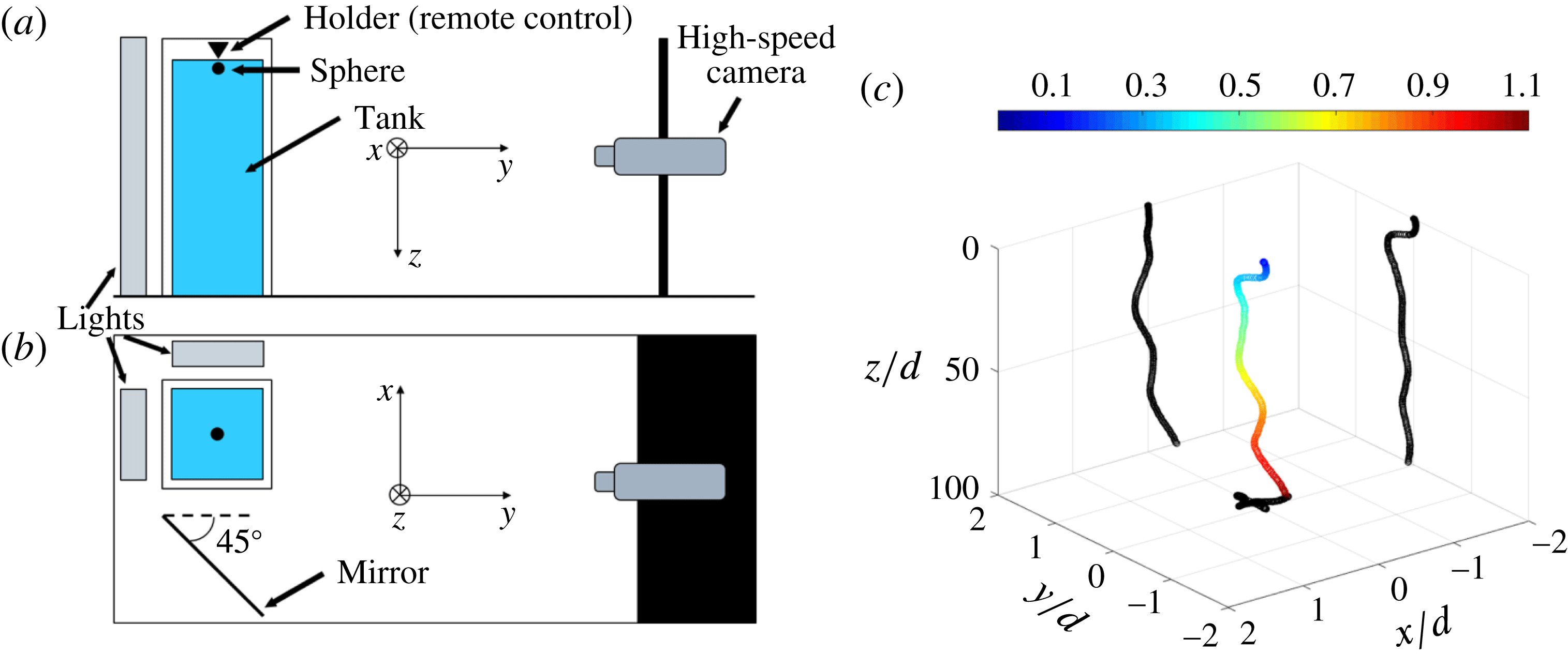
Once released, the sphere motion was recorded by a Phantom V341 high-speed camera (Zeiss Makro-Planar T*
 $2/50~\text{mm}$
ZF lens), at a
 $2560\times 1100~\text{px}^{2}$
resolution with a frame rate of 1000 fps. A mirror placed at
 $45^{\circ }$
with respect to the tank enabled the simultaneous recording of front and side views with a single camera. The selected recording window resulted into a conversion factor of
 $0.3~\text{mm}~\text{px}^{-1}$
. The results reported in this paper are obtained by averaging ten independent trials. A 15 min settling time was imposed between each test to ensure the water was completely at rest before the spheres’ release. This value was chosen as a compromise between the large number of executed tests and the fluid quiescence necessity. Horowitz & Williamson (Reference Horowitz and Williamson2010a
) imposed a 2 h settling time, showing how disturbances in the fluid may lead to large random transverse motion. No justification for such large time was given. Conversely, Truscott, Epps & Munns (Reference Truscott, Epps and Munns2016) justified their 30 min settling time performing particle image velocimetry measurements of the flow field following an experimental run. However, buoyant spheres (Horowitz & Williamson Reference Horowitz and Williamson2010a
; Truscott et al.
Reference Truscott, Epps and Munns2016) may be more impacted by residual disturbances rather than the large density stainless steel spheres used in this work. Moreover, blank tests were executed varying the imposed settling time, showing no appreciable differences. A post-processing analysis of the recorded videos, carried out with the commercial software MATLAB®, allowed the reconstruction of the time-resolved three-dimensional (3-D) trajectory of the falling spheres, with the
 $z$
-axis aligned with the gravity
 $g$
and the
 $x$
and
 $y$
coordinates referring to the horizontal plane. The evolution of the sphere velocity was deduced from the time derivative of these trajectories (see figure 2
c). Details of the used algorithm and measurements uncertainties are presented in appendix A. Velocity uncertainties (95 % confidence level) lower than 5 % of the corresponding terminal velocity were evaluated for all the analysed spheres. Notice that the exploited tank was not tall enough to let the large diameter spheres reach their terminal velocity. Measurements presented in § 4 should therefore be regarded as qualitative results for
 $Re_{\infty }\geqslant 2\times 10^{4}$
. A new experimental set-up is currently under construction to overcome this issue.
In addition to the sphere motion measurement, high magnification videos were performed to investigate the behaviour of the air plastron during the fall. In that case, a
 $2048\times 1152~\text{px}^{2}$
recording window (Sigma 180 mm F2.8 APO Macro EX DG OS lens) and a 1300 fps recording speed were used. Only the front plane was recorded, and the corresponding spatial resolution was
 $0.06~\text{mm}~\text{px}^{-1}$
.
2.2 The super-hydrophobic coatings
A wide range of manufacturing procedures have been developed to produce SH surfaces (see e.g. Zhang et al. Reference Zhang, Shi, Niu, Jiang and Wang2008; Bhushan & Jung Reference Bhushan and Jung2011, for a review), from chemical vapour deposition (Lau et al. Reference Lau, Bico, Teo, Chhowalla, Amaratunga, Milne, McKinley and Gleason2003) to costless mechanical sanding of naturally water-repellent materials (Nilsson, Daniello & Rothstein Reference Nilsson, Daniello and Rothstein2010) to cite but a few. Depending on the selected technique, either regular or random patterns of micron-sized and/or nano-sized structures can be produced at the surface. In most cases, the samples studied are flat surfaces. However, a large number of the techniques mentioned above are not suitable as far as curved surfaces are concerned. This is the reason why a spray coating method (McHale et al. Reference McHale, Shirtcliffe, Evans and Newton2009; Aljallis et al. Reference Aljallis, Sarshar, Datla, Sikka, Jones and Choi2013; Kim et al. Reference Kim, Kim and Park2015) was used to produce the SH spheres. The SH properties were obtained by depositing a commercially available product, Ultra-Ever Dry® (UltraTech International 2017). To this end, a specific manufacturing procedure was designed as follows:
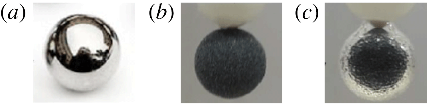
(i) the surface of the reference sphere was first cleaned with acetone then rinsed with double-distilled water and finally dried (see figure 3 a),
(ii) an etch primer (Ultra-Ever Dry® bottom coating) was uniformly sprayed over the surface,
(iii) an intermediate layer made of a carbon-based powder was deposited onto the surface in order to control the surface texture (see figure 3 b),
(iv) the etch primer was sprayed again over the intermediate layer and then air dried for at least 1 h with a double purpose: firmly stick the powder to the surface and provide a consistent material for the SH coating to bond,
(v) the SH properties were obtained by spraying the Ultra-Ever Dry® top coating over the surface and letting it dry for at least 2 h.
Two different carbon-based powders with grade P220 and P80 were employed as intermediate layers in this study. The resulting coatings are labelled SH-220 and SH-80, respectively. In addition, SH spheres without intermediate layer were produced by skipping steps 3 and 4 of the described procedure. This coating will be referred to as SH-NAR (no additional roughness) in the following. Compared to the smooth spheres, the deposit of the SH coating increases both mass and diameter, which have been measured with an accuracy of 0.1 mg and
 $10~\unicode[STIX]{x03BC}\text{m}$
, respectively. Accordingly, the resulting density ratio between sphere and water (
 $\unicode[STIX]{x1D701}=\unicode[STIX]{x1D70C}_{s}/\unicode[STIX]{x1D70C}_{f}$
), which is one of the main driving parameters of the falling motion (Ern et al.
Reference Ern, Risso, Fabre and Magnaudet2012) lies within [6.2–7.8]. The high values of
 $\unicode[STIX]{x1D701}$
achieved in this study imply that the sphere motion is predominantly vertical (see figure 6 in Ern et al. (Reference Ern, Risso, Fabre and Magnaudet2012) where this behaviour is referred to as mode A) as illustrated by the scales of movement in figure 2(c). Note also that the size of the roughness deposited on the sphere surface is not high enough to promote the laminar-to-turbulent transition of the boundary layer (Achenbach Reference Achenbach1974) which would lead to the so-called drag crisis (see figure 1). Details of the properties of the produced spheres and measurement uncertainties are provided in appendix A.
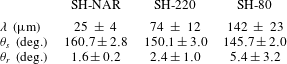
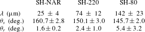
In addition, SH flat plates were produced following the same manufacturing procedure in order to analyse the properties of the SH coatings. Results obtained from the combination of confocal microscopy (see figure 4) and contact angle measurements are outlined in table 1, which emphasises the change in surface roughness
 $\unicode[STIX]{x1D706}$
as a function of the grade of the intermediate layer. Due to the completely random spatial distribution of the powder particles,
 $\unicode[STIX]{x1D706}$
was chosen as the representative dimension of the roughness elements (see e.g. Alamé & Mahesh Reference Alamé and Mahesh2018). All produced surfaces are characterised by high static contact angle
 $\unicode[STIX]{x1D703}_{s}$
and low roll-off angle
 $\unicode[STIX]{x1D703}_{r}$
(indicative of small contact angle hysteresis), which are symptomatic of the so-called Cassie–Baxter state. This is well supported by the presence of the air plastron around SH spheres once immersed in water as demonstrated in figure 3(c).
Images taken during the manufacturing procedure of a
 $d=10~\text{mm}$
SH sphere illustrating: (a) reference stainless steel sphere, (b) intermediate layer made of a carbon-based powder, (c) air plastron around the surface of the SH sphere once immersed in water.

Major properties of the produced SH coatings.
 $\unicode[STIX]{x1D706}$
, root-mean-square surface roughness.
 $\unicode[STIX]{x1D703}_{s}$
, static contact angle.
 $\unicode[STIX]{x1D703}_{r}$
, roll-off angle. The reported uncertainties represent the 95 % confidence level.
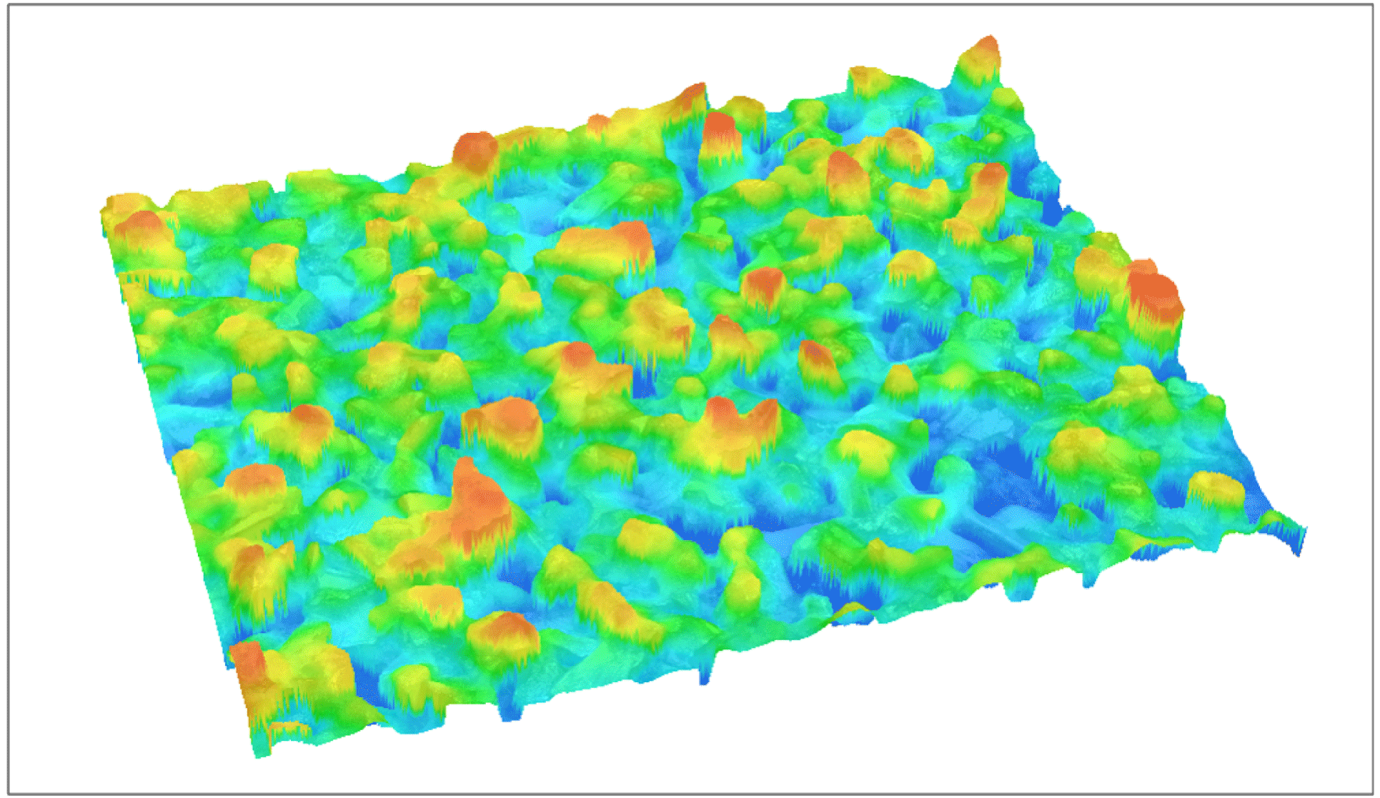
Confocal microscopy analysis of a portion (
 $1.5\times 1.0~\text{mm}$
) of a flat plate covered with the SH-220 coating. The colour scale (blue-to-red) indicates the surface roughness
 $(0{-}170~\unicode[STIX]{x03BC}\text{m})$
. Notice the completely random spatial distribution of the powder particles.

3 Plastron deformation
For the remainder of the paper, the symbol
 $^{\star }$
denotes dimensionless variables where the time
 $t_{0}=\sqrt{d/((\unicode[STIX]{x1D701}-1)g)}$
and the velocity
 $V_{0}=\sqrt{(\unicode[STIX]{x1D701}-1)gd}$
are used as scaling parameters to account for gravity/buoyancy effects (Jenny et al.
Reference Jenny, Dušek and Bouchet2004). Accordingly, the typical Reynolds number is defined as
 $Re=\unicode[STIX]{x1D70C}_{f}V_{0}d/\unicode[STIX]{x1D707}$
, with
 $\unicode[STIX]{x1D707}$
the dynamic viscosity of water. Note that in this study
 $\unicode[STIX]{x1D701}$
is kept roughly constant, which means that the sphere diameter,
 $d$
, is the main control parameter.
As mentioned previously, the amount of vorticity generated at the surface of the body is a key ingredient for what concerns the development of the wake. The production of vorticity at the sphere surface is expected to be concentrated within the laminar boundary layer, which is characterised by its thickness
 $\unicode[STIX]{x1D6FF}\sim dRe^{-1/2}$
. The vorticity generated in the boundary layer can be approximated by
 $\unicode[STIX]{x1D714}\sim \unicode[STIX]{x0394}U/\unicode[STIX]{x1D6FF}$
with
 $\unicode[STIX]{x0394}U$
the typical velocity jump across the boundary layer (Batchelor Reference Batchelor1967). In the case of a slippery wall,
 $\unicode[STIX]{x0394}U\sim V_{0}-V_{g}$
where
 $V_{g}$
is the slip velocity. Introducing the slip-length model and approximating the slip length by the characteristic dimension of the surface roughness
 $\unicode[STIX]{x1D706}$
(Ybert et al.
Reference Ybert, Barentin, Cottin-Bizonne, Joseph and Bocquet2007) yields
 $V_{g}\sim \unicode[STIX]{x1D706}u_{\unicode[STIX]{x1D70F}}^{2}/\unicode[STIX]{x1D708}$
, with
 $u_{\unicode[STIX]{x1D70F}}$
the friction velocity and
 $\unicode[STIX]{x1D708}=\unicode[STIX]{x1D707}/\unicode[STIX]{x1D70C}_{f}$
the fluid kinematic viscosity. Assuming the viscous drag to account for 10 % of the total drag (sub-critical regime) we obtain
 $u_{\unicode[STIX]{x1D70F}}=kV_{0}$
, with
 $k=O(10^{-1})$
. Plugging these expressions together yields:
 $$\begin{eqnarray}\unicode[STIX]{x1D714}^{\star }=A\left(1-k\frac{\unicode[STIX]{x1D706}}{\unicode[STIX]{x1D6FF}_{\unicode[STIX]{x1D708}}}\right)\frac{d}{\unicode[STIX]{x1D6FF}},\end{eqnarray}$$
with
 $\unicode[STIX]{x1D6FF}_{\unicode[STIX]{x1D708}}=\unicode[STIX]{x1D708}/u_{\unicode[STIX]{x1D70F}}$
the viscous length scale and
 $A=O(1)$
. For a given sphere diameter, this relationship predicts that the production of vorticity decreases linearly with the slip length, which is assimilated to the surface roughness here. However, it is important to recall that this prediction is based on the assumption that the air layer encapsulating the sphere is non-deformable. Details on the derivation of (3.1) and its implications are given in appendix B.
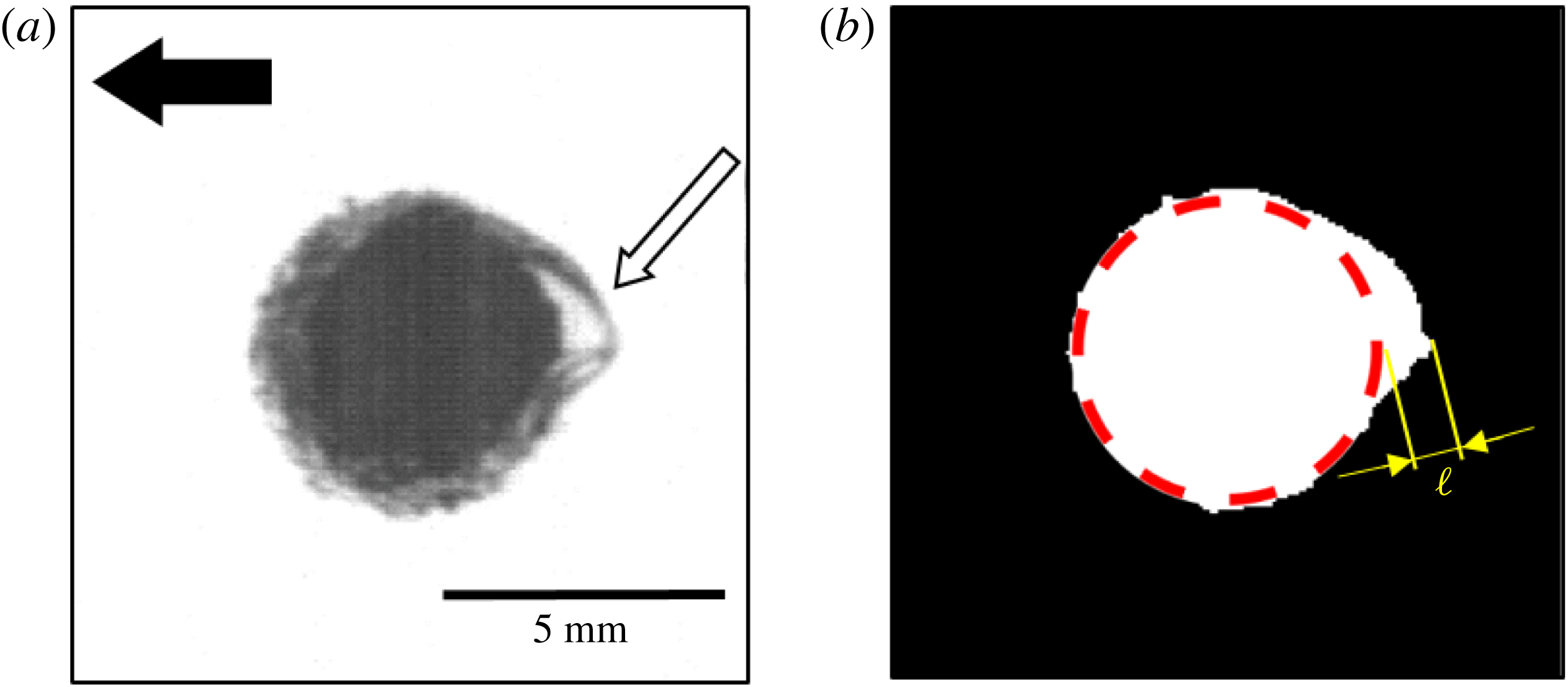
(a) Typical image recorded during the fall of an SH-80 sphere (
 $d=5~\text{mm}$
) using the high magnification configuration. The black arrow denotes the gravity direction. The white arrow indicates the region where the plastron deformation is visible. (b) Binarised image resulting from the contour finding algorithm used to compute the aspect ratio
 $\unicode[STIX]{x1D712}$
. The red dashed line symbolises the sphere. The variable
 $\ell$
denotes the typical length scale of the observed protrusion.

Figure 5 shows a typical snapshot of an SH-80 sphere (
 $d=5~\text{mm}$
) during its falling motion using the high magnification configuration. This image clearly illustrates the deformation of the air plastron as testified by the presence of a huge protrusion located at the backside of the sphere. The plastron deformation can be quantified by introducing the aspect ratio
 $\unicode[STIX]{x1D712}$
such that:
 $$\begin{eqnarray}\unicode[STIX]{x1D712}=\frac{d_{eq}}{d},\end{eqnarray}$$
where
 $d_{eq}$
denotes an equivalent diameter defined as follows:
 $$\begin{eqnarray}d_{eq}=2\sqrt{\frac{{\mathcal{S}}}{\unicode[STIX]{x03C0}}},\end{eqnarray}$$
with
 ${\mathcal{S}}$
the surface area delineated by the deformed interface. Based on the MATLAB® image processing toolbox, a contour finding algorithm has been developed to estimate
 ${\mathcal{S}}$
. The output of this algorithm applied to the image shown in figure 5(a) is illustrated in figure 5(b). In practice,
 ${\mathcal{S}}$
is estimated via the computation of the white area. As shown in figure 6, the plastron shape is extremely sensitive to the sphere diameter or equivalently
 $Re$
. Indeed, while the sequence in figure 6(a) (
 $d=5~\text{mm}$
) is characterised by the presence of a single protrusion, the sequence in figure 6(b) (
 $d=20~\text{mm}$
) reveals the presence of multiple air pockets. Note however that the typical length scale,
 $\ell$
, of the protrusions observed in this study (see figure 5
b) remains roughly constant (
 ${\approx}1.5\pm 0.5~\text{mm}$
) independently of
 $d$
and
 $\unicode[STIX]{x1D706}$
. From the image post-processing of the high magnification configuration, it is found that
 $\unicode[STIX]{x1D712}$
decreases from around 1.2 for the smallest SH spheres (i.e.
 $d=5~\text{mm}$
) to approximately 1 for the largest SH spheres (i.e.
 $d=25~\text{mm}$
). In other words, although the local normalised curvature
 $d/\ell$
increases with the sphere diameter, at the same time the global shape of the plastron tends to be spherical. This means that the idealised shape assumed to derive the expression (3.1) is more likely to be achieved for the largest sphere diameter in this study.
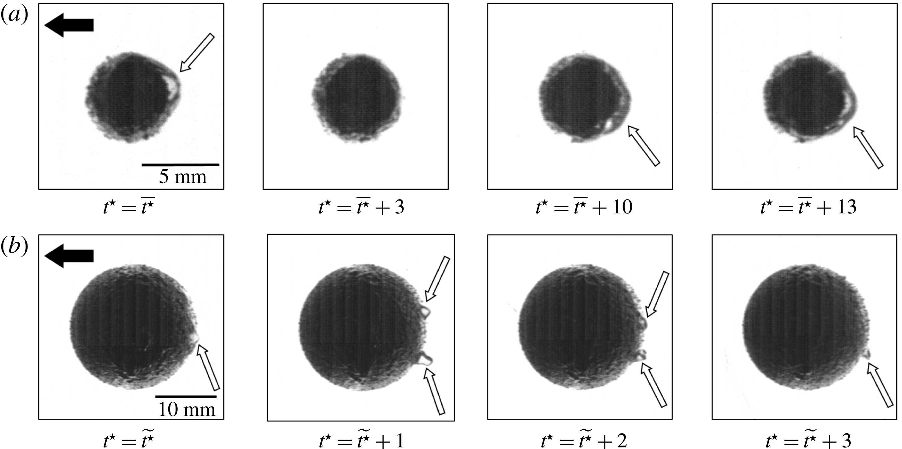
Typical snapshots recorded in high magnification configuration illustrating the movement and deformation of the air plastron (indicated by white arrows) around SH-80 coated spheres. (a)
 $d=5~\text{mm}$
, (b)
 $d=20~\text{mm}$
. The black arrows represent the gravity direction. The variables
 $\overline{t^{\star }}$
and
 $\widetilde{t^{\star }}$
designate two time origins chosen randomly.

As emphasised in figures 5 and 6, the interface distortion occurs at the backside of the spheres, which undergoes the massive separation of the laminar boundary layer typical of the sub-critical regime. This suggests that the pressure deficit induced by the flow separation promotes the (partial) suction of the air entrapped in the surface roughness. The change in
 $\unicode[STIX]{x1D712}$
is therefore the result of the local competition between the separation-induced suction (
 ${\sim}\unicode[STIX]{x1D70C}V_{0}^{2}$
) and the capillary pressure (
 ${\sim}\unicode[STIX]{x1D6FE}/d$
, with
 $\unicode[STIX]{x1D6FE}$
the water/air surface tension), which can be qualitatively represented by introducing the Weber number such as:
 $$\begin{eqnarray}{\mathcal{W}}e=\frac{\unicode[STIX]{x1D70C}_{f}V_{0}^{2}d}{\unicode[STIX]{x1D6FE}}.\end{eqnarray}$$
It is worth noticing that this definition differs from that proposed by Seo et al. (Reference Seo, García-Mayoral and Mani2015) who quantified the flow/interface interaction in a turbulent channel flow with viscosity-based variables. Indeed, the wake of the sphere studied here is predominated by the form drag. However, one can show that
 ${\mathcal{W}}e^{+}={\mathcal{W}}ek^{2}\unicode[STIX]{x1D6FF}_{\unicode[STIX]{x1D708}}/d$
, where
 ${\mathcal{W}}e^{+}$
is the Weber number in wall units as introduced by Seo et al. (Reference Seo, García-Mayoral and Mani2015). In this study,
 ${\mathcal{W}}e^{+}\approx 10^{-3}$
. Furthermore, it is found that
 $\unicode[STIX]{x1D706}^{+}=\unicode[STIX]{x1D706}u_{\unicode[STIX]{x1D70F}}/\unicode[STIX]{x1D708}\leqslant 15$
which is lower than the critical slip length where plastron failure is expected to occur as predicted by Seo et al. (Reference Seo, García-Mayoral and Mani2015). This is consistent with the fact that we did not observe the release of air bubbles in the wake except when the sphere hits the bottom of the tank.
According to the definition of
 $V_{0}$
:
 $$\begin{eqnarray}{\mathcal{W}}e=\frac{\unicode[STIX]{x1D70C}_{f}g}{\unicode[STIX]{x1D6FE}}(\unicode[STIX]{x1D701}-1)d^{2}.\end{eqnarray}$$
Recalling that here
 $\unicode[STIX]{x1D701}$
is roughly constant, this expression implies that the sphere diameter is also the main control parameter of the flow/interface interaction.
An important remark has to be made here about the relationship between
 $\unicode[STIX]{x1D712}$
and
 ${\mathcal{W}}e$
. Although both of them characterise the interaction between the plastron and the local stresses induced by the wake,
 $\unicode[STIX]{x1D712}$
is perfectly suited to deliver an a posteriori quantitative description of the interface deformation. However, a reliable estimation of
 $\unicode[STIX]{x1D712}$
suffers from a severe limitation. Indeed, the computation of
 $\unicode[STIX]{x1D712}$
is based on a two-dimensional projection of a phenomenon which is likely three-dimensional. Unfortunately, the out-of-plane deformations, although perceptible (see the supplementary movie available at https://doi.org/10.1017/jfm.2018.480), are hidden due to the sphere opacity. This is the reason why in this study it is more convenient to use
 ${\mathcal{W}}e$
rather than
 $\unicode[STIX]{x1D712}$
. In fact, since
 ${\mathcal{W}}e$
is set a priori, it should be regarded as a qualitative indicator of plastron deformation. Let us now derive a relation linking
 $\unicode[STIX]{x1D712}$
and
 ${\mathcal{W}}e$
. Assuming that
 $d_{eq}\approx d+\ell$
, equation (3.2) can be reformulated as follows:
 $$\begin{eqnarray}\unicode[STIX]{x1D712}=1+\frac{\ell }{d}.\end{eqnarray}$$
The approximated relation
 $d_{eq}\approx d+\ell$
provides
 $\unicode[STIX]{x1D712}$
variations from around 1.2 for the small diameter spheres toward the unitary value for the largest diameter spheres, in good agreement with the definition given in (3.3). Since
 $\ell$
is found almost constant:
 $$\begin{eqnarray}{\mathcal{W}}e\sim (\unicode[STIX]{x1D712}-1)^{-2}.\end{eqnarray}$$
In other words, low values of
 ${\mathcal{W}}e$
are associated with large
 $\unicode[STIX]{x1D712}$
and vice versa. The implications of this relationship will be discussed further in § 4.3.
The visualisations provided in figures 5 and 6 suggest that the air plastron compliance and its dynamics are intimately connected to the wake. This raises the issue of a possible feedback of the plastron motion and deformation onto the flow. Somehow, the plastron deformation evidenced in this study shares some properties of freely rising bubbles (Ellingsen & Risso Reference Ellingsen and Risso2001). Basically, the main difference is that bubbles adapt their entire shape whereas here only a thin layer is compliant. It is the reason why the maximum values of
 $\unicode[STIX]{x1D712}$
observed here (
 ${\approx}1.2$
) are much lower compared to those of fully deformable bodies (Mougin & Magnaudet Reference Mougin and Magnaudet2002b
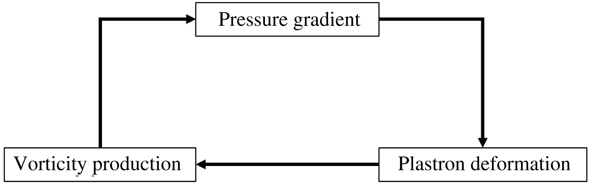
). Nevertheless, it is reasonable to assume that the physical mechanisms driving the body/flow interaction are comparable, at least qualitatively. In figure 7, a schematic description of this interaction is proposed: the unsteady pressure gradient induced by the massive separation around the falling sphere promotes the deformation and the movement of the air plastron. This modification of the boundary conditions may alter significantly the production of vorticity at the body surface and accordingly the intensity of vorticity within the wake (see e.g. Mougin & Magnaudet Reference Mougin and Magnaudet2002b
; Legendre et al.
Reference Legendre, Lauga and Magnaudet2009), which in turn may impact the pressure gradient. The feedback loop described in figure 7 suggests that the plastron deformation could have a sizeable effect on the sphere wake since the hydrodynamic forces experienced by the body are intimately linked to both pressure and vorticity distributions.
A possible driving mechanism of the mutual interaction between the flow and the air plastron.

4 Hydrodynamic performance
So far, our observations reveal that the plastron shape is extremely sensitive to the stresses induced by the wake. To proceed further, we now investigate the influence of physical parameters on the hydrodynamic forces, i.e. lift and drag, experienced by the falling spheres, with the goal of emphasising the feedback of plastron deformation onto the flow. The effects of three possible parameters could be assessed: (i)
 $Re$
which characterises the wake, (ii)
 $\unicode[STIX]{x1D706}/d$
which is representative of the slip and (iii)
 ${\mathcal{W}}e$
(or equivalently
 $\unicode[STIX]{x1D712}$
) which describes the interface deformation. Note that due to their definitions,
 $Re$
and
 ${\mathcal{W}}e$
cannot be set independently. However, as mentioned previously, we expect the physical influence of
 $Re$
to be negligible (at least over the range studied here) in comparison of that of
 ${\mathcal{W}}e$
. This point will be discussed further in § 4.3. Based on this assumption, we focus mostly on the role of
 $\unicode[STIX]{x1D706}/d$
and
 ${\mathcal{W}}e$
in the following.
4.1 Vertical motion
Let us start by investigating the fall of a sphere for which large deformations happen, i.e. at low
 ${\mathcal{W}}e$
. The time histories of the normalised vertical falling velocity
 $v_{z}^{\star }$
and acceleration
 $\dot{v}_{z}^{\star }=\text{d}v_{z}^{\star }/\text{d}t^{\star }$
for the smallest spheres (
 $d=5~\text{mm}$
) are displayed in figures 8 and 9, comparing the reference and the SH-80 coated surfaces. Starting from rest the sphere first accelerates yielding an increase of
 $v_{z}^{\star }$
and then reaches its terminal velocity
 $v_{z\infty }^{\star }$
once transient effects vanish. Note that, in this study, since
 $\unicode[STIX]{x1D701}\approx 7$
, the vertical motion could be well approximated by solving the following equation (Mordant & Pinton Reference Mordant and Pinton2000):
 $$\begin{eqnarray}\left(\unicode[STIX]{x1D701}+\frac{1}{2}\right)\dot{v}_{z}^{\star }=1-\frac{3C_{D}}{4}v_{z}^{\star 2},\end{eqnarray}$$
where the empirical law
 $C_{D}(Re)$
given by Cheng (Reference Cheng2009) was considered (see figure 1). In (4.1), the left-hand side term is the acceleration weighted by the added mass, while the right-hand side terms represent the gravity/buoyancy and the drag force respectively. For the sake of simplicity, the term accounting for the Stokes memory effects was not considered (see Mordant & Pinton (Reference Mordant and Pinton2000) for full details). Note that at release time, i.e.
 $t^{\star }=0$
, the vertical velocity is zero, and subsequently the drag term is null. This, combined with the exclusion of memory effects, implies that the predicted velocity is expected to be slightly overestimated shortly after the sphere release and in the initial part of the sphere drop.
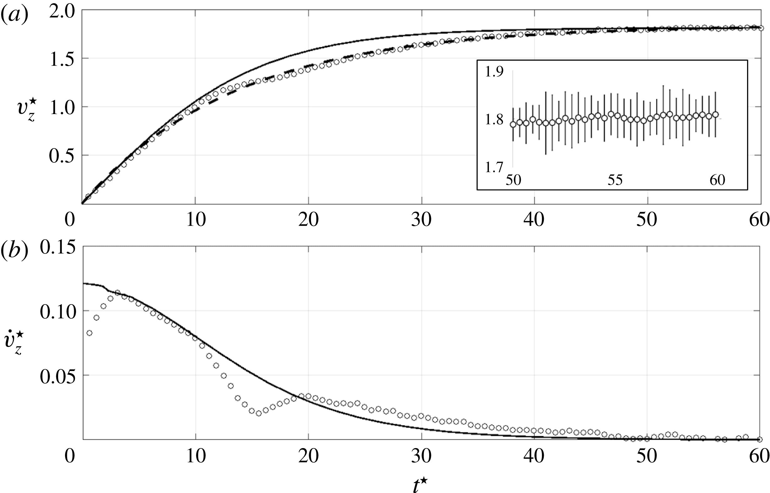
Time evolution of the vertical velocity (a) and acceleration (b) of the
 $d=5~\text{mm}$
reference (smooth) spheres. ○, Experimental data (for the sake of readability, 1 point out of 2 is reported). Solid line: prediction according to (4.1). Dashed line: fitted model according to (4.4) (Mordant & Pinton Reference Mordant and Pinton2000). The inset shows the error bars (95 % confidence level) in the terminal velocity region.

For the reference sphere, a good agreement between the predicted and the measured falling velocity is observed at the early stage of the motion and in the steady state as well (see figure 8
a). However, a significant departure arises within the range
 $t^{\star }\in [10;40]$
. The experimental velocity drop is induced by an acceleration decrease occurring between
 $t^{\star }\approx 10$
and
 $t^{\star }\approx 20$
(see figure 8
b). Such a phenomenon has been reported by other authors and is induced by the onset of instabilities in the wake of the sphere, which promotes a sudden drag increase (Jenny et al.
Reference Jenny, Dušek and Bouchet2004). This point will be discussed further in § 4.2. More surprisingly, from
 $t^{\star }\approx 20$
to
 $t^{\star }\approx 40$
the measured sphere acceleration exceeds its predicted value, which balances the previous acceleration reduction and enables the reference sphere to reach its predicted terminal velocity, provided that
 $v_{z\infty }^{\star }=\int _{0}^{\infty }\dot{v}_{z}^{\star }\,\text{d}t^{\star }$
.
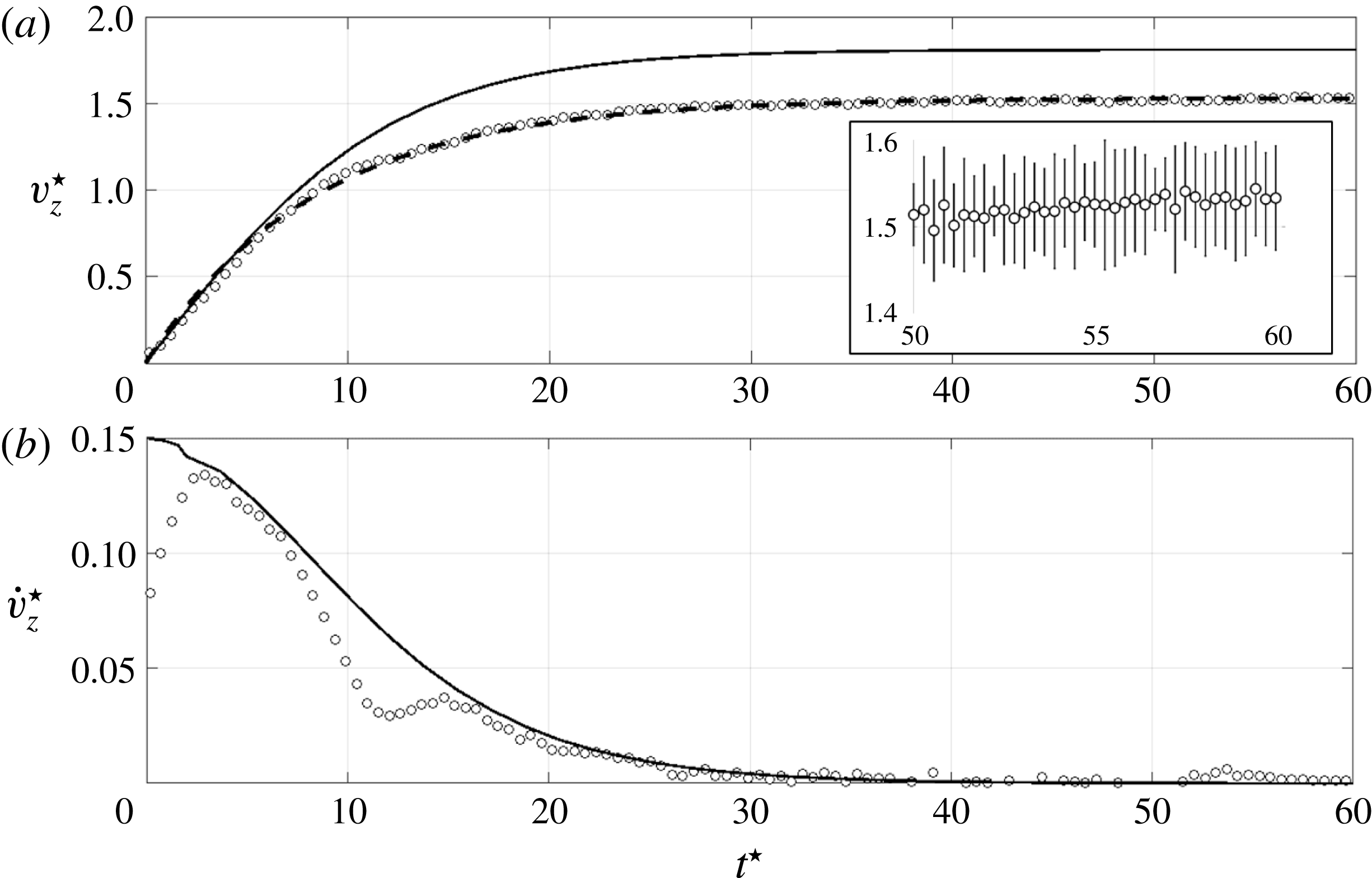
For the SH sphere, figure 9(b) similarly evidences an acceleration decrease. However, the departure from the predicted acceleration occurs at
 $t^{\star }\approx 7$
, which means that the SH coating promotes the onset of instabilities earlier than the reference sphere. Moreover, unlike the reference sphere, the measured acceleration then collapses onto the predicted trend beyond
 $t^{\star }\approx 15$
. Accordingly, the terminal velocity achieved by the SH sphere is much lower than its predicted value as emphasised in figure 9(a). In the specific case displayed in figures 8 and 9, i.e.
 $d=5~\text{mm}$
, this yields an increase of terminal drag coefficient due to the SH coating, since (4.1) reduces to
 $C_{D\infty }=4/3v_{z\infty }^{\star 2}$
once transient effects vanish. This result agrees with the findings of Ahmmed et al. (Reference Ahmmed, Patience and Kietzig2016) who reported drag increase of laser-textured SH spheres at comparable Reynolds numbers.
Time evolution of the vertical velocity (a) and acceleration (b) of the
 $d=5~\text{mm}$
SH-80 coated spheres. ○, Experimental data (for the sake of readability, 1 point out of 2 is reported). Solid line: prediction according to (4.1). Dashed line: fitted model according to (4.4) (Mordant & Pinton Reference Mordant and Pinton2000). The inset shows the error bars (95 % confidence level) in the terminal velocity region.

4.2 Lift force
In what follows we focus on the flow-induced loads experienced by the spheres, starting with lift. Since lift force results from the asymmetric distribution of vorticity released in the wake, it is a very well suited indicator of instability onset. The time history of the lift coefficient
 $C_{L}=8|L|/(\unicode[STIX]{x1D70C}_{f}v_{z}^{2}\unicode[STIX]{x03C0}d^{2})$
, where
 $|L|$
is the lift force magnitude, was estimated by solving the generalised Kirchhoff equations (Mougin & Magnaudet Reference Mougin and Magnaudet2002a
) following the methodology described in detail by Shew, Poncet & Pinton (Reference Shew, Poncet and Pinton2006). The interested reader can find some details about the strategy followed for the
 $C_{L}$
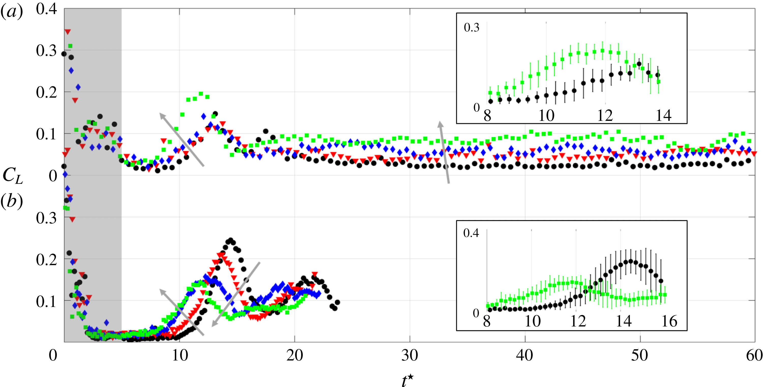
evaluation and its connection with the transversal motion in appendix C. Figure 10 shows the evolution of
 $C_{L}$
calculated from our experimental data for
 $d=5~\text{mm}$
(
 ${\mathcal{W}}e\approx 20$
) and
 $d=20~\text{mm}$
(
 ${\mathcal{W}}e\approx 360$
) spheres. Note that the signal-to-noise ratio is too low at the early stage of motion (shaded zone) for the lift force estimation to be reliable. At the starting of motion,
 $C_{L}$
is almost null, meaning that the wake is axisymmetric and accordingly the trajectory is vertical. Then,
 $C_{L}$
suddenly increases as a result of the loss of axisymmetry of the wake, which originates from instabilities arising in the wake (Magnaudet & Eames Reference Magnaudet and Eames2000; Horowitz & Williamson Reference Horowitz and Williamson2010b
). These instabilities promote path unsteadiness (see figure 2
c) together with a vertical velocity decrease with respect to the prediction, as discussed in § 4.1. However, the amplitude of path excursion is moderate due to lift fluctuation damping caused by the high
 $\unicode[STIX]{x1D701}$
values considered in this study. Once lift fluctuations vanish,
 $C_{L}$
remains almost constant, which implies the sphere to follow an oblique trajectory. Note that for the
 $d=20~\text{mm}$
spheres, the tank is not tall enough for the lift force to reach its steady state. Nevertheless, the wake transition as well as the damping of the lift fluctuation are clearly visible.
Time history of the lift coefficient of the (a)
 $d=5~\text{mm}$
and (b)
 $d=20~\text{mm}$
spheres (for the sake of readability, 1 point out of 2 is reported). ●, Reference (smooth) sphere. ▾, SH-NAR coating. ♦, SH-220 coating. ▪, SH-80 coating. The grey arrows indicate increasing roughness thickness. The shaded region identifies the portion of time where lift estimation is corrupted by the signal-to-noise ratio. The two insets show the error bars (95 % confidence level) in the wake instability occurrence region.

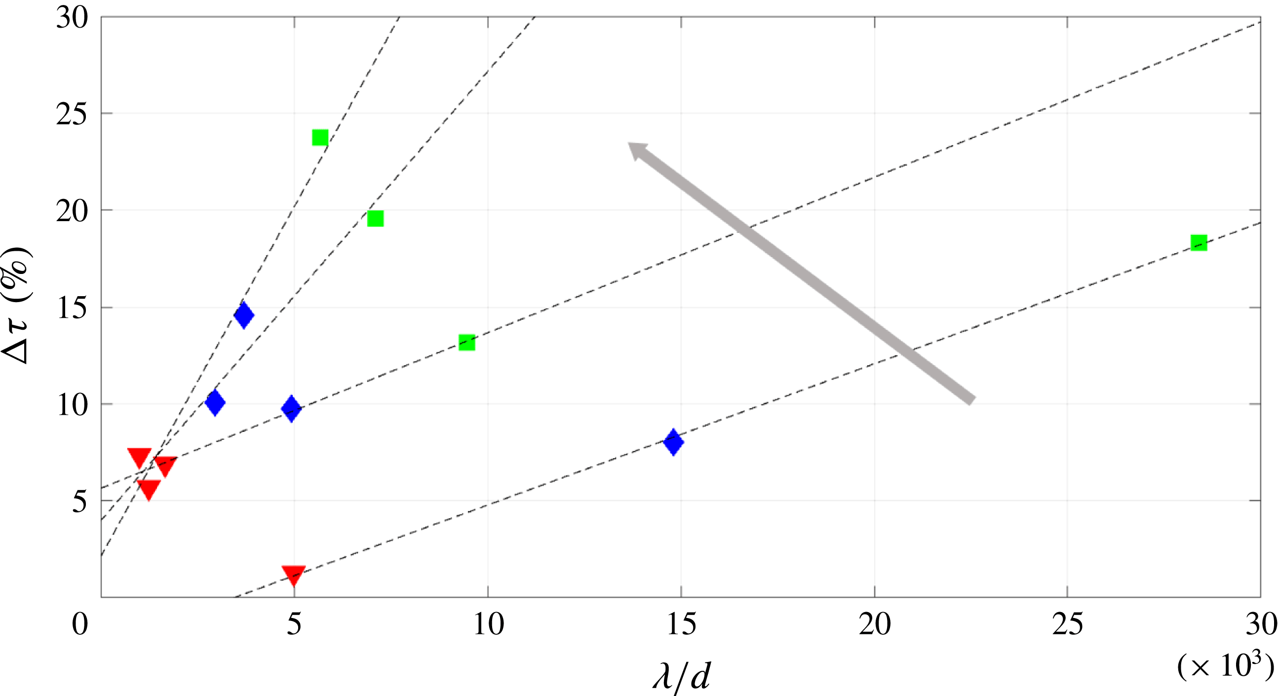
Effect of surface properties on the characteristic time at which wake instabilities appear. ▾, SH-NAR coating. ♦, SH-220 coating. ▪, SH-80 coating. Dashed lines: best fit of (4.2) in the least-mean square sense. The grey arrow indicates increasing
 ${\mathcal{W}}e$
. For the sake of readability, only results for
 $d=5$
, 15, 20 and 25 mm are reported.

We now introduce
 $\unicode[STIX]{x1D70F}$
as the characteristic time at which the wake instability occurs. In practice,
 $\unicode[STIX]{x1D70F}$
is estimated as the time where the condition
 $C_{L}=0.05$
is first met. This threshold value was chosen in order to ensure the detection of the instability to be above the experimental uncertainties of the lift coefficient. The evolution of
 $\unicode[STIX]{x0394}\unicode[STIX]{x1D70F}=1-\unicode[STIX]{x1D70F}^{SH}/\unicode[STIX]{x1D70F}^{ref}$
(with superscripts
 $SH$
and
 $ref$
referring to SH coating and smooth surface, respectively) is displayed in figure 11 with respect to the dimensionless roughness
 $\unicode[STIX]{x1D706}/d$
for different sphere diameters. It appears that the data are well fitted by a linear relationship:
 $$\begin{eqnarray}\unicode[STIX]{x0394}\unicode[STIX]{x1D70F}\approx \unicode[STIX]{x1D6FC}_{\unicode[STIX]{x1D70F}}\frac{\unicode[STIX]{x1D706}}{d},\end{eqnarray}$$
with
 $\unicode[STIX]{x1D6FC}_{\unicode[STIX]{x1D70F}}$
the slope of the law. In any case, the SH coatings trigger wake instability earlier than the reference spheres. Our findings agree with the results of Jenny et al. (Reference Jenny, Dušek and Bouchet2004) and Fernandes et al. (Reference Fernandes, Risso, Ern and Magnaudet2007) who reported earlier transition of asymmetric bodies. In a similar fashion, the imperfect sphericity induced by the interface distortion may trigger the wake instabilities more rapidly.


Figure 12 shows the variation of
 $\unicode[STIX]{x1D6FC}_{\unicode[STIX]{x1D70F}}$
as a function of
 ${\mathcal{W}}e$
. It is found that
 $\unicode[STIX]{x1D6FC}_{\unicode[STIX]{x1D70F}}\sim {\mathcal{W}}e^{m}$
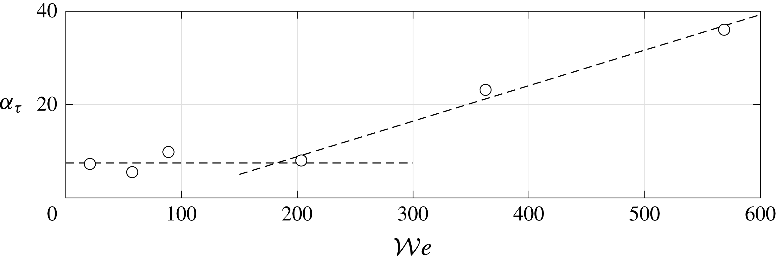
over the available range of operating conditions tested in this study. Surprisingly, this plot reveals an abrupt change of the power law exponent
 $m$
, which varies from 0 to 1, around a critical value
 ${\mathcal{W}}e_{c}=180$
such that
 $$\begin{eqnarray}\left.\begin{array}{@{}ll@{}}\displaystyle \unicode[STIX]{x1D6FC}_{\unicode[STIX]{x1D70F}}=\unicode[STIX]{x1D6FC}_{\unicode[STIX]{x1D70F}0} & \text{if }{\mathcal{W}}e<{\mathcal{W}}e_{c},\\ \displaystyle \unicode[STIX]{x1D6FC}_{\unicode[STIX]{x1D70F}}=\unicode[STIX]{x1D6FC}_{\unicode[STIX]{x1D70F}0}\left(2\frac{{\mathcal{W}}e}{{\mathcal{W}}e_{c}}-1\right) & \text{if }{\mathcal{W}}e\geqslant {\mathcal{W}}e_{c},\end{array}\right\}\end{eqnarray}$$
with
 $\unicode[STIX]{x1D6FC}_{\unicode[STIX]{x1D70F}0}\approx 7.5$
. As evidenced in figure 10, the change in
 $\unicode[STIX]{x1D6FC}_{\unicode[STIX]{x1D70F}}$
observed at
 ${\mathcal{W}}e_{c}$
coincides with a significant modification of the magnitude of both the lift fluctuations during the transient phase and the lift force in the steady regime. For
 ${\mathcal{W}}e<{\mathcal{W}}e_{c}$
(figure 10
a), SH coatings tend to increase lift, especially in the steady state regime. On the contrary, for
 ${\mathcal{W}}e\geqslant {\mathcal{W}}e_{c}$
(figure 10
b), the lift amplitude is reduced. Remember that the lift force is intimately related to the intensity of vorticity around the body. Accordingly, our findings suggest that the high interface distortion which is achieved on average when
 ${\mathcal{W}}e<{\mathcal{W}}e_{c}$
leads to an increase of the amount of vorticity released in the wake. On the contrary, the production of vorticity seems to be mitigated when the condition
 ${\mathcal{W}}e\geqslant {\mathcal{W}}e_{c}$
is met, which would imply that the expression (3.1) is assessed.
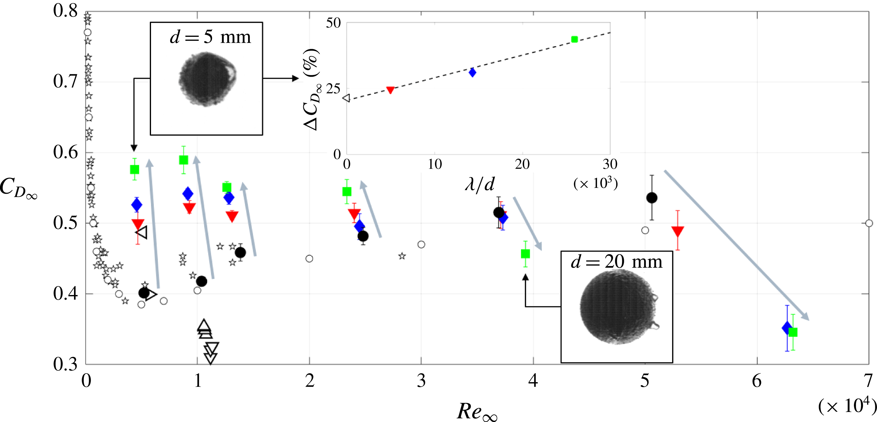
Terminal drag coefficient
 $C_{D\infty }$
as a function of terminal Reynolds number
 $Re_{\infty }$
for all the investigated spheres. ●, Reference (smooth) sphere. ▾, SH-NAR coating. ♦, SH-220 coating. ▪, SH-80 coating. ✩, spheres falling rectilinearly (Horowitz & Williamson Reference Horowitz and Williamson2010a
). ▹, Reference sphere (Ahmmed et al.
Reference Ahmmed, Patience and Kietzig2016). ◃, SH sphere (Ahmmed et al.
Reference Ahmmed, Patience and Kietzig2016). ▵,
 $d=25~\text{mm}$
reference spheres (McHale et al.
Reference McHale, Shirtcliffe, Evans and Newton2009). ▿,
 $d=25~\text{mm}$
SH spheres with air plastron (McHale et al.
Reference McHale, Shirtcliffe, Evans and Newton2009). ○, Experimental data from Lapple & Sheperd (Reference Lapple and Sheperd1940). The error bars represent the 95 % confidence level. The grey arrows indicate increasing surface roughness thickness. The inset shows the terminal drag coefficient variation with respect to the reference sphere as a function of the non-dimensional roughness
 $\unicode[STIX]{x1D706}/d$
for the spheres in the
 $Re_{\infty }\approx 0.5\times 10^{4}$
region.

4.3 Drag force
Let us now illustrate the consequences on the terminal drag coefficient
 $C_{D\infty }$
, which is displayed in figure 13 as a function of the terminal Reynolds number
 $Re_{\infty }=v_{z\infty }^{\star }Re$
. As mentioned previously, for the largest spheres (
 $Re_{\infty }\geqslant 2\times 10^{4}$
) the tank is not tall enough for the steady state to be achieved. In the worst case (
 $d=25~\text{mm}$
), the maximum measurable vertical velocity is 15 % lower than the terminal velocity predicted by (4.1). To overcome this issue, the terminal velocity
 $v_{z\infty }^{\star }$
was inferred by best fitting, in the least-mean square sense, the data with the following model proposed by Mordant & Pinton (Reference Mordant and Pinton2000):
 $$\begin{eqnarray}v_{z}^{\star }=v_{z\infty }^{\star }(1-\text{e}^{-\unicode[STIX]{x1D6FD}t^{\star }}),\end{eqnarray}$$
where
 $v_{z\infty }^{\star }$
and
 $\unicode[STIX]{x1D6FD}$
are the fit parameters. Figures 8 and 9 demonstrate the relevance of the model expressed in (4.4). It is worth noting that due to the limitations of our experimental set-up, the measurements presented in figure 13 for
 $Re_{\infty }\geqslant 2\times 10^{4}$
should be regarded as qualitative results emphasising the relative influence of plastron properties on drag. A new experimental set-up is currently under design to properly address this issue. For assessment purposes, data obtained by Lapple & Sheperd (Reference Lapple and Sheperd1940), Horowitz & Williamson (Reference Horowitz and Williamson2010a
) (for spheres falling rectilinearly) as well as those estimated from the results given by McHale et al. (Reference McHale, Shirtcliffe, Evans and Newton2009) and Ahmmed et al. (Reference Ahmmed, Patience and Kietzig2016) for smooth and SH spheres have also been reported. As far as reference (smooth) spheres are concerned, a fairly good agreement between our measurements and the data reported in previous studies is observed over the overlapping
 $Re_{\infty }$
range, with the exception of the work of McHale et al. (Reference McHale, Shirtcliffe, Evans and Newton2009). Beyond
 $Re_{\infty }\approx 3\times 10^{4}$
, our data deviate slightly from that of Lapple & Sheperd (Reference Lapple and Sheperd1940) which may be due to the fitting procedure.
For what concerns SH coatings, both interface deformation (i.e.
 ${\mathcal{W}}e$
) and slip (i.e.
 $\unicode[STIX]{x1D706}/d$
) have a sizeable influence on
 $C_{D\infty }$
. We introduce
 $\unicode[STIX]{x0394}C_{D}=1-C_{D\infty }^{SH}/C_{D\infty }^{ref}$
to characterise the drag change induced by the surface properties. The inset in figure 13 shows the evolution of
 $\unicode[STIX]{x0394}C_{D}$
for the smallest sphere (i.e.
 $d=5~\text{mm}$
). For comparison, the drag change reported by Ahmmed et al. (Reference Ahmmed, Patience and Kietzig2016) at a comparable
 $Re_{\infty }$
is also displayed. It is worth noting the excellent agreement between our data and those of Ahmmed et al. (Reference Ahmmed, Patience and Kietzig2016), whose SH spheres are characterised by a nano-sized surface roughness. This plot suggests that the drag change is well approximated by the following law:
 $$\begin{eqnarray}\unicode[STIX]{x0394}C_{D}=\unicode[STIX]{x1D6FC}_{D}\frac{\unicode[STIX]{x1D706}}{d}+\unicode[STIX]{x0394}C_{D0},\end{eqnarray}$$
where
 $\unicode[STIX]{x0394}C_{D0}$
represents the drag change extrapolated at virtually zero surface roughness and
 $\unicode[STIX]{x1D6FC}_{D}$
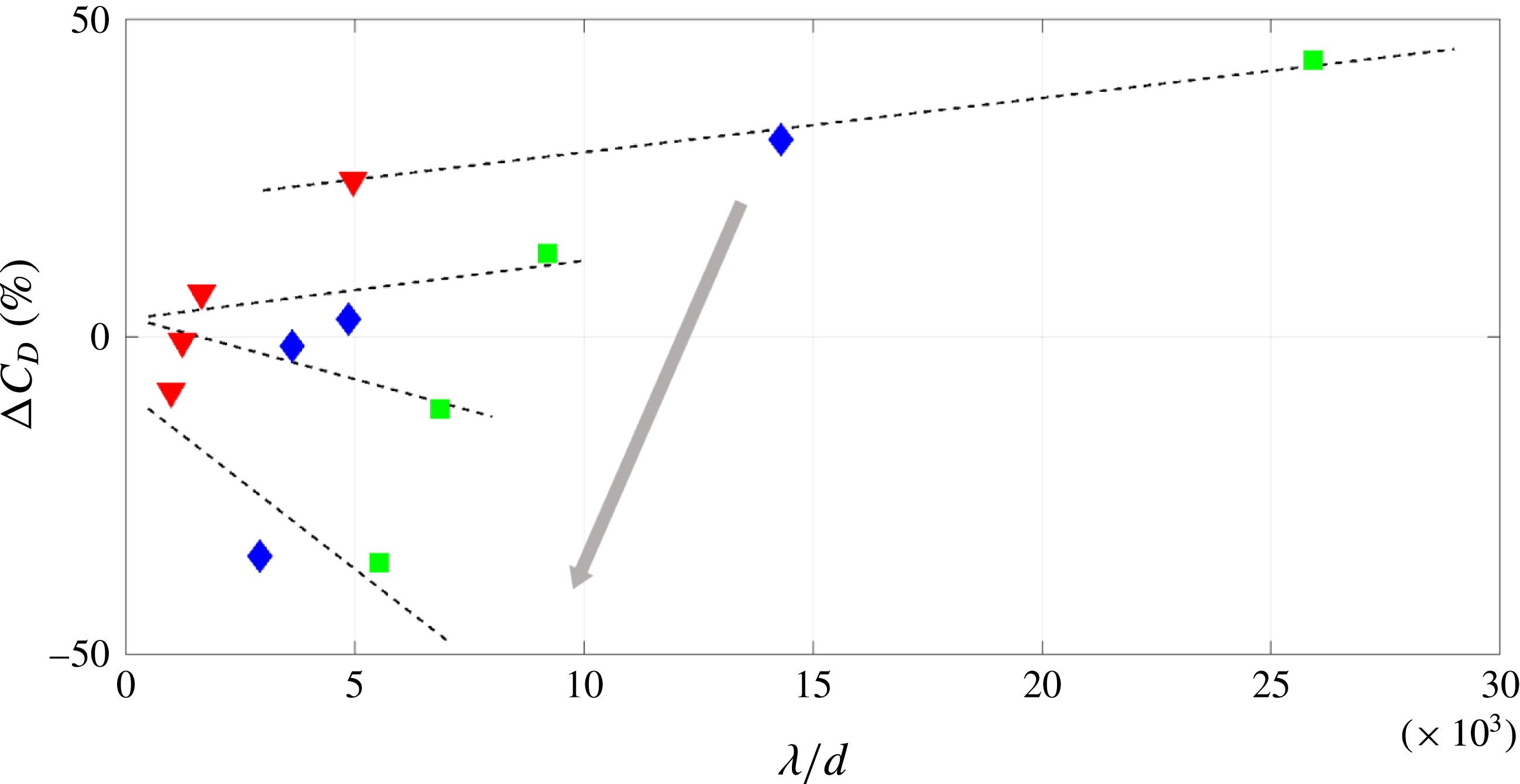
stands for the drag rate of change. As evidenced in figure 14, this trend applies also for the other spheres tested in this study. Drag increase with respect to the reference by up to
 $+45\,\%$
is found for the smallest spheres (low
 ${\mathcal{W}}e$
), whereas a significant drag reduction down to
 $-35\,\%$
is noticed for the largest spheres (high
 ${\mathcal{W}}e$
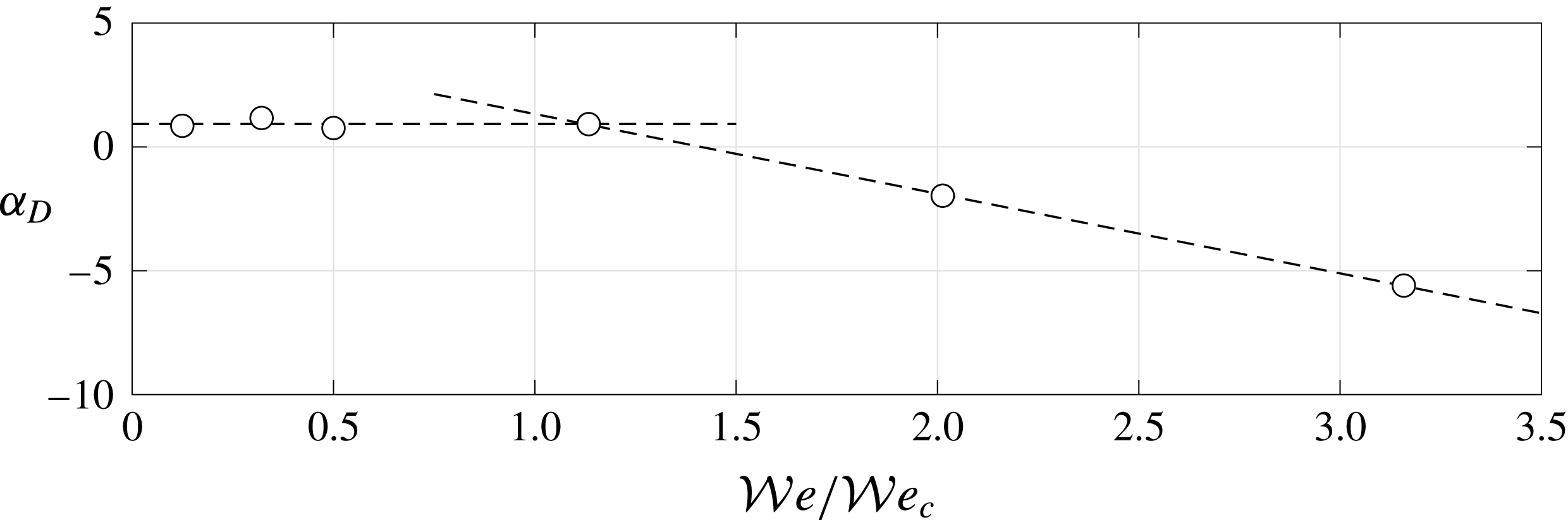
). This opposite trend is even more evident in figure 15, which displays the evolution of
 $\unicode[STIX]{x1D6FC}_{D}$
as a function of
 ${\mathcal{W}}e$
normalised by the critical value
 ${\mathcal{W}}e_{c}$
.
Terminal drag coefficient variation with respect to the reference sphere as a function of the non-dimensional roughness. ▾, SH-NAR coating. ♦, SH-220 coating. ▪, SH-80 coating. The dashed lines highlight the linear behaviour (see (4.5)). The grey arrow indicates increasing
 ${\mathcal{W}}e$
. For the sake of readability, only results for
 $d=5$
, 15, 20 and 25 mm are reported.


Much as was observed for
 $\unicode[STIX]{x1D6FC}_{\unicode[STIX]{x1D70F}}$
, it is found that
 $\unicode[STIX]{x1D6FC}_{D}\sim {\mathcal{W}}e^{m}$
. Once again, an abrupt change of trend is clearly visible at
 ${\mathcal{W}}e_{c}$
such that:
 $$\begin{eqnarray}\left.\begin{array}{@{}ll@{}}\displaystyle \unicode[STIX]{x1D6FC}_{D}=\unicode[STIX]{x1D6FC}_{D0} & \text{if }{\mathcal{W}}e<{\mathcal{W}}e_{c},\\ \displaystyle \unicode[STIX]{x1D6FC}_{D}=4.5-3.2\frac{{\mathcal{W}}e}{{\mathcal{W}}e_{c}} & \text{if }{\mathcal{W}}e\geqslant {\mathcal{W}}e_{c},\end{array}\right\}\end{eqnarray}$$
with
 $\unicode[STIX]{x1D6FC}_{D0}\approx 0.93$
. For
 ${\mathcal{W}}e<{\mathcal{W}}e_{c}$
,
 $\unicode[STIX]{x1D6FC}_{D}$
is roughly constant and positive meaning that drag increases with increasing plastron thickness. On the contrary, for
 ${\mathcal{W}}e<{\mathcal{W}}e_{c}$
,
 $\unicode[STIX]{x1D6FC}_{D}$
becomes negative which yields the drag reduction observed in figure 13.
It is worth noting that the drag changes observed in this study encompass the different trends reported in previous works (McHale et al.
Reference McHale, Shirtcliffe, Evans and Newton2009; Ahmmed et al.
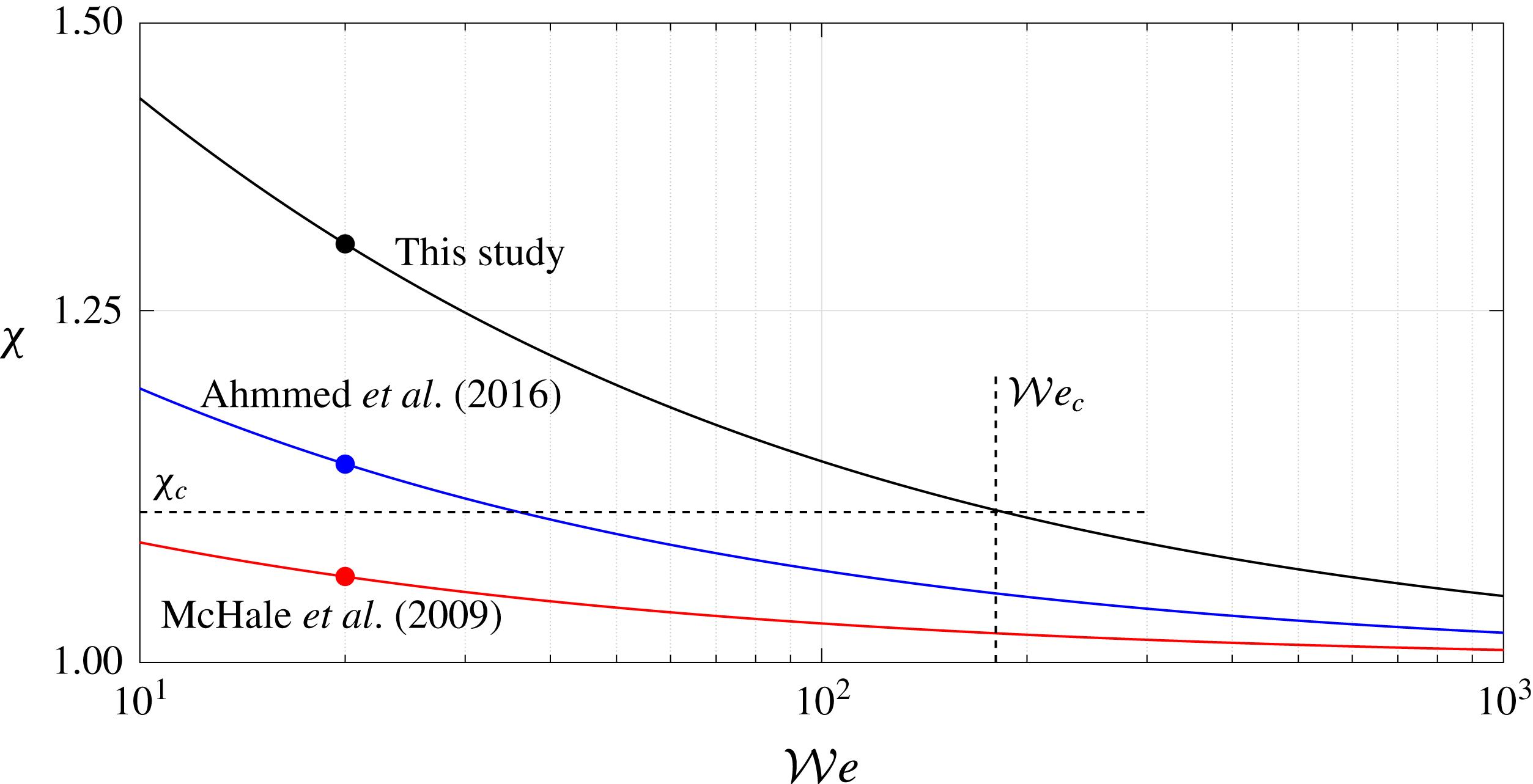
Reference Ahmmed, Patience and Kietzig2016). Taking into account the plastron deformation might provide an attractive way to explain these results within a unified framework. Indeed, according to (3.5), the Weber number characterising the studies of McHale et al. (Reference McHale, Shirtcliffe, Evans and Newton2009) and Ahmmed et al. (Reference Ahmmed, Patience and Kietzig2016) is approximately 20, which is comparable to the smallest value reached in this work. Based on our results, one would expect drag increase, which is not reported by McHale et al. (Reference McHale, Shirtcliffe, Evans and Newton2009). This illustrates that a comprehensive relationship between
 ${\mathcal{W}}e$
and
 $\unicode[STIX]{x1D712}$
needs to be properly established. In fact, a possible explanation of these apparently discordant results arises by developing (3.7) one step further. To this end, equation (3.5) injected into (3.6) yields:
 $$\begin{eqnarray}\unicode[STIX]{x1D712}=1+\sqrt{\frac{\unicode[STIX]{x1D70C}_{f}(\unicode[STIX]{x1D701}-1)g\ell ^{2}}{\unicode[STIX]{x1D6FE}}}{\mathcal{W}}e^{-1/2}.\end{eqnarray}$$
This expression takes into account the influence of
 $\unicode[STIX]{x1D701}$
, whose values are approximately 2.2 in the work of Ahmmed et al. (Reference Ahmmed, Patience and Kietzig2016) (PTFE spheres) and 1.2 in the study of McHale et al. (Reference McHale, Shirtcliffe, Evans and Newton2009) (acrylic spheres). Based on the assumption that the magnitude of the air layer protrusions,
 $\ell$
, is comparable to that observed here, figure 16 shows the evolution of
 $\unicode[STIX]{x1D712}$
according to (4.7). In correspondence to
 ${\mathcal{W}}e_{c}$
(see figure 12), we introduce a critical aspect ratio
 $\unicode[STIX]{x1D712}_{c}\approx 1.1$
. Based on our findings, a highly deformed plastron, i.e.
 $\unicode[STIX]{x1D712}>\unicode[STIX]{x1D712}_{c}$
, yields a drag increase, whilst a plastron that is almost spherical on average, i.e.
 $\unicode[STIX]{x1D712}<\unicode[STIX]{x1D712}_{c}$
, results in drag mitigation. Focusing our attention on the
 ${\mathcal{W}}e\approx 20$
region, it appears clearly that the aspect ratio featuring the study of McHale et al. (Reference McHale, Shirtcliffe, Evans and Newton2009) lies below
 $\unicode[STIX]{x1D712}_{c}$
. This perfectly agrees with the drag reduction these authors reported. Conversely, drag increase observed in this study and in the work of Ahmmed et al. (Reference Ahmmed, Patience and Kietzig2016) falls within the region of highly deformed plastron, i.e.
 $\unicode[STIX]{x1D712}>\unicode[STIX]{x1D712}_{c}$
. Altogether, our results clearly emphasise that, under the investigated operating conditions, the plastron compliance plays a key role in the performance of SH surfaces. Obviously, further efforts are required to confirm our findings and extrapolate them over a broader range of operating conditions.
Variation of the aspect ratio
 $\unicode[STIX]{x1D712}$
as a function of
 ${\mathcal{W}}e$
according to (4.7). Solid black: this study. Solid blue: Ahmmed et al. (Reference Ahmmed, Patience and Kietzig2016). Solid red: McHale et al. (Reference McHale, Shirtcliffe, Evans and Newton2009). The vertical dashed line indicates the critical Weber number
 ${\mathcal{W}}e_{c}$
, whilst the horizontal dashed line represents its corresponding critical aspect ratio
 $\unicode[STIX]{x1D712}_{c}$
. The dots symbolise the Weber number region where the studies can be compared (
 ${\mathcal{W}}e\approx 20$
).

5 Concluding remarks
In this work, free falling experiments of super-hydrophobic spheres were carried out. To do so, super-hydrophobic coatings were deposited over stainless steel spheres via a spray method suitable for large scale applications. The surface roughness was controlled by embedding micron-sized powders with different particle size during the manufacturing process. A particular attention has been placed on the influence of the deformation of the air layer encapsulating the sphere in the Cassie–Baxter state. To this end, the sphere motion was analysed to investigate the hydrodynamic performance in the so-called sub-critical regime.
A first outcome of this study is the evidence of plastron deformation in response to the separation-induced stresses experienced in the wake of the spheres. The competition between the pressure deficit and the surface tension was estimated quantitatively using the aspect ratio
 $\unicode[STIX]{x1D712}$
of the observed body and qualitatively by introducing the Weber number
 ${\mathcal{W}}e$
. The analysis of highly resolved visualisations indicates that the plastron adopts an oblate shape at low
 ${\mathcal{W}}e$
, whilst it tends to be spherical on average at high
 ${\mathcal{W}}e$
.
The second outcome of this work relates to the feedback of the plastron deformation on the flow. Indeed, it has been found that the plastron compliance has a sizeable influence on the wake development. In a first stage, the transient fall was studied through the time history of the lift coefficient, which is used as a footprint of the amount of vorticity generated during the sphere motion. Compared to smooth spheres used as reference, it has been observed that the onset of the wake instabilities is triggered earlier by the super-hydrophobic coatings. The time at which the instabilities are detected decreases linearly with the slippage effect, which is controlled by changing the surface roughness. Our results highlight an abrupt change of scaling law around a critical Weber number,
 ${\mathcal{W}}e_{c}\approx 200$
. A simple model was used to derive the critical aspect ratio
 $\unicode[STIX]{x1D712}_{c}$
where the condition
 ${\mathcal{W}}e={\mathcal{W}}e_{c}$
is met. The steady state is then investigated via the terminal drag coefficient which is compared to values reported in others studies. In comparison to drag measured for the reference spheres, significant drag increase is obtained for highly deformed interface achieved for
 $\unicode[STIX]{x1D712}>\unicode[STIX]{x1D712}_{c}$
, whereas low deformation obtained for
 $\unicode[STIX]{x1D712}<\unicode[STIX]{x1D712}_{c}$
results in drag mitigation.
Even though the proposed scenario provides an attractive way to explain and unify apparently dissonant results reported in previous works, it requires additional studies with the aim of delivering more reliable SH surface models. Moreover, our study should be extended to a broader range of operating conditions. The motivations of doing so are threefold: (i) delineate regimes where the plastron compliance cannot be neglected, (ii) discriminate the effect of
 $Re_{\infty }$
and
 ${\mathcal{W}}e$
and (iii) assess the relationship between
 ${\mathcal{W}}e$
and the aspect ratio
 $\unicode[STIX]{x1D712}$
outside the sub-critical regime. Altogether, our findings suggest that the plastron compliance may be a fundamental phenomenon involved in the production of vorticity at the body surface, which in turns deeply impacts the wake. A full understanding of the physical mechanisms at play during the wake transition and the terminal state would require further investigations. Finally, it should be determined whether or not our findings can be extrapolated to other flows (e.g. pressure-driven flows) over SH surfaces.
Acknowledgements
This work was supported by the Direction Générale de l’Armement (DGA), Ministère de la Défense, République Française and the Agence Nationale de la Recherche (ANR) through the Investissements d’Avenir program under the Labex CAPRYSSES Project (ANR-11-LABX-0006-01). The financial support of the Région Centre/Val de Loire through the regional project Modif’Surf is also gratefully acknowledged. N.M. wishes to thank Professor A. Bottaro and Dr R. García-Mayoral for fruitful discussions.
Supplementary movie
Supplementary movie is available at https://doi.org/10.1017/jfm.2018.480.
Appendix A. Measurement uncertainties and algorithm validation
In this appendix, we provide details about the experimental measurement uncertainties and the post-processing technique used to evaluate both the velocity and the acceleration.
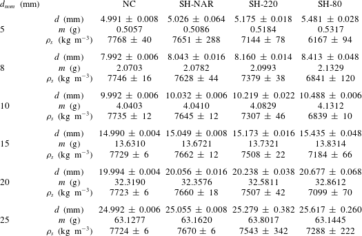
Measured properties of the analysed spheres.
 $d_{nom}$
, nominal diameter.
 $d$
, actual diameter.
 $m$
, mass (measurement accuracy 0.1 mg).
 $\unicode[STIX]{x1D70C}_{s}$
, density. Reported uncertainties represent the
 $95\,\%$
confidence level.
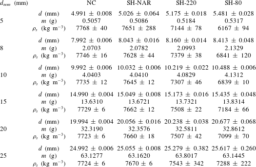
Table 2 shows the measured properties of all the analysed spheres. The nominal diameter of the stainless steel bearing spheres ranges from 5 to 25 mm. The actual sphere diameter was measured along at least five different directions, with a resolution of
 $10~\unicode[STIX]{x03BC}\text{m}$
. The reported uncertainties on
 $d$
, which represent the
 $95\,\%$
confidence level, remain lower than
 $2\,\%$
of the respective average value in all cases, testifying to the satisfactory sphericity of the coated spheres. All the SH coatings determine a
 $d$
increase with respect to the corresponding reference sphere, with a maximum
 $+10\,\%$
in the SH-80 coating case. Masses were evaluated by a single measurement with a Mettler Toledo AB104-S analytical balance, with an accuracy of 0.1 mg. The largest mass augmentation (
 $+5\,\%$
) with respect to the corresponding reference sphere was reached with the SH-80 coating. The deposition of the SH coatings results in a decrease of the sphere density with respect to the reference stainless steel sphere (down to
 $-20\,\%$
). The largest uncertainties of the sphere densities (
 $95\,\%$
confidence level) were approximately
 $4\,\%$
of the respective average value.
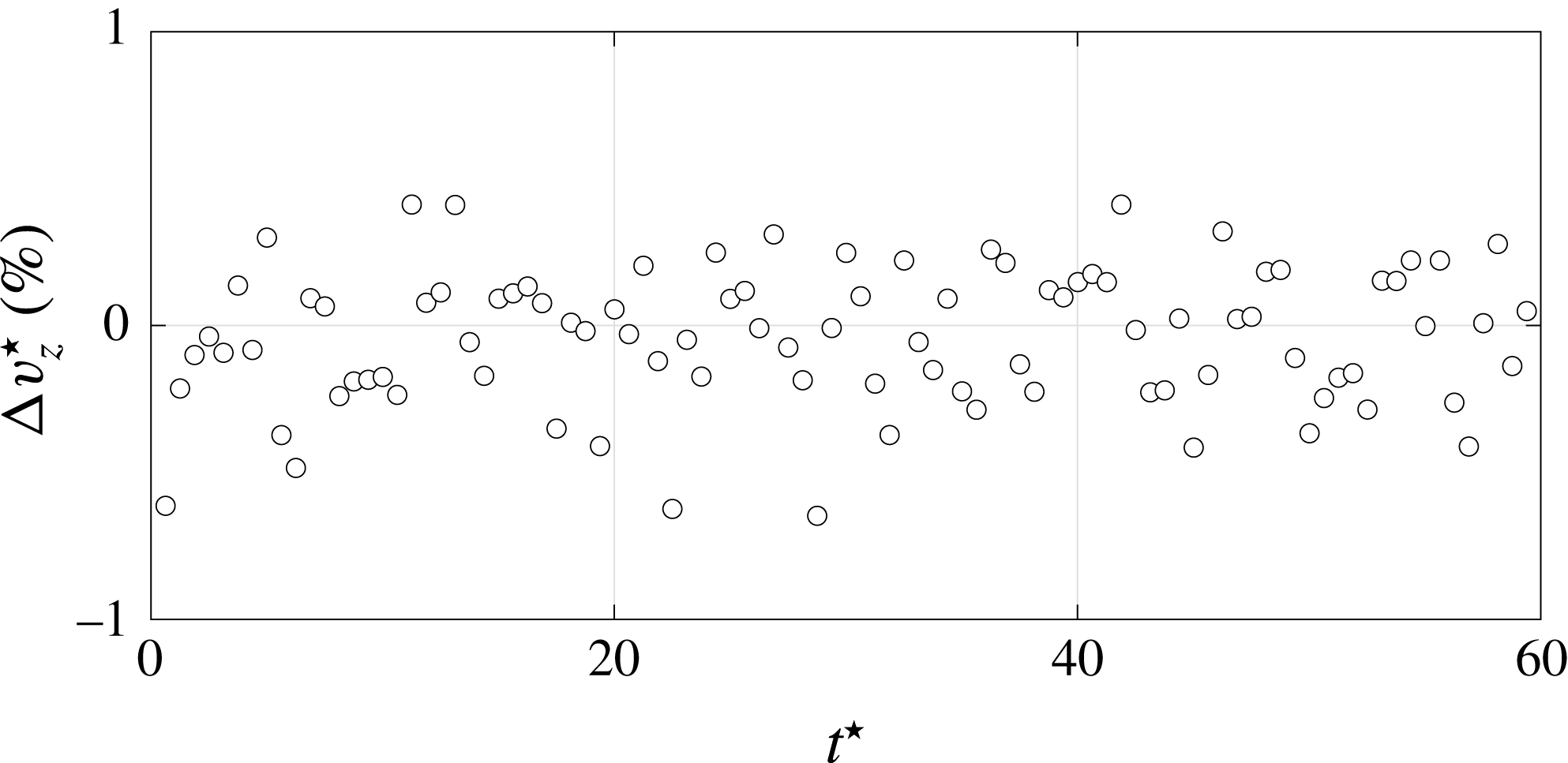
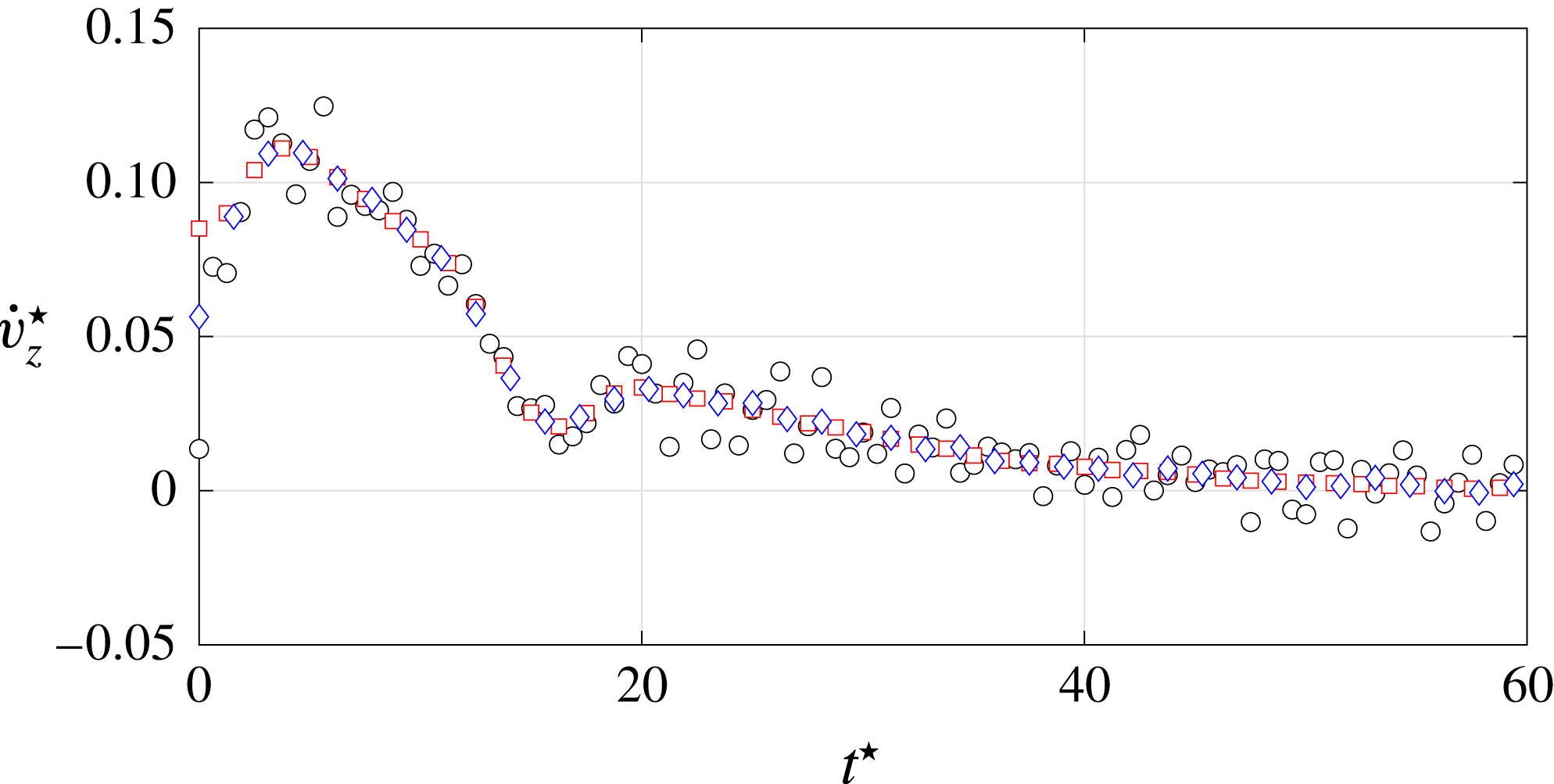
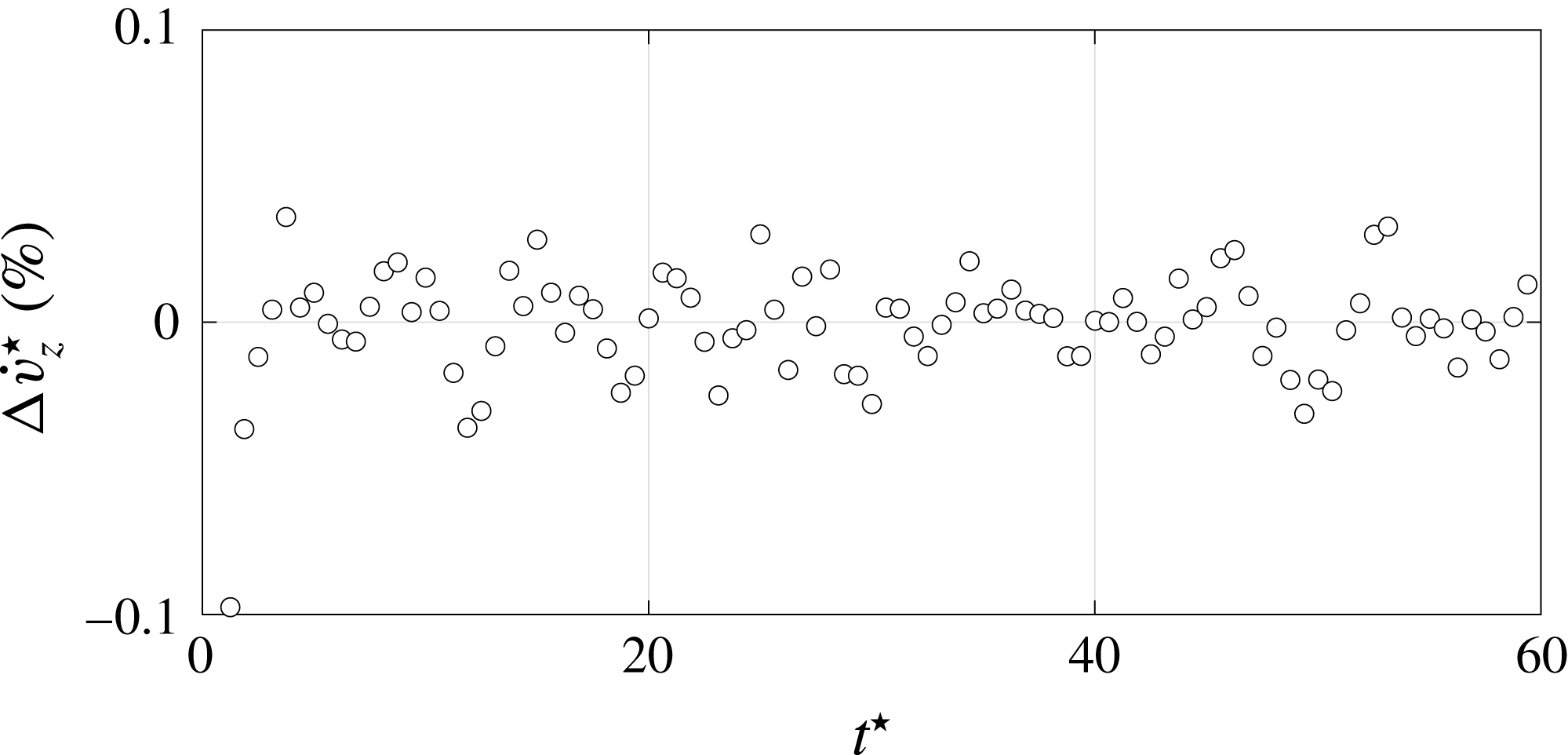
Once the 3-D sphere trajectories were available, velocities and accelerations were calculated by a time derivative. For time-resolved experimental data, noticeable error propagation may be obtained. Two techniques were therefore compared in order to achieve reliable velocity and acceleration information. Firstly, we performed an estimation of velocity and acceleration via a central finite difference scheme (subscript FD): an a posteriori filtering of the obtained derivative is performed in the cases where it is deemed necessary, as explained in the following. Secondly, we followed the approach originally proposed by Reinsch (Reference Reinsch1967) and recently developed by Epps, Truscott & Techet (Reference Epps, Truscott and Techet2010) where position data are fitted with a smoothing spline (subscript SPL), then the time derivation is performed directly on the spline. The method consist on finding the spline with the least roughness possible, given an error tolerance. The more the fitted spline captures the experimental data noise, the more its roughness increases. A roughness–error tolerance graph can thus be generated, making possible the detection of a critical error tolerance that corresponds to the optimal spline fit. Figure 17 shows the percentage difference of the vertical velocity
 $\unicode[STIX]{x0394}v_{z}^{\star }=(v_{zFD}^{\star }-v_{zSPL}^{\star })/v_{z\infty SPL}^{\star }$
evaluated by the two techniques in the case of the reference sphere analysed in figure 8. Since no filtering was performed in the finite difference case, figure 17 clearly shows that, under the investigated operating conditions of our study, the two techniques give approximately the same estimation of the velocity profile. Velocity variations lower than
 $1\,\%$
of the respective terminal velocity were evaluated in all cases. Conversely, a second derivative step amplified the measurement error to a non-satisfactory level in the finite difference case. Figure 18 shows the marked amplification of the experimental noise with respect to the acceleration evaluated by the spline fitting technique. A large gap between the two techniques is especially noticed at the very beginning of the drop. The acceleration estimated by the finite difference scheme thus needs to be filtered to adequately reduce the experimental noise to a satisfactory level. In detail, a Savitzky–Golay filter with a third-order polynomial and a window length equal to 25 experimental points was used. Figures 18 and 19 testify the good agreement between the two techniques in the case of the reference sphere analysed in figure 8. Deviations
 $\unicode[STIX]{x0394}\dot{v}_{z}^{\star }=(\dot{v}_{zFD}^{\star }-\dot{v}_{zSPL}^{\star })/\dot{v}_{zSPL,max}^{\star }$
lower than
 $0.1\,\%$
of the acceleration largest value are obtained during the whole drop. A more marked gap between the filtered finite difference scheme and the spline method is still visible at the very beginning of the drop, but it does not influence the wake instability region at larger
 $t^{\star }$
, which is the focus of the discussion in § 4.2. Since the uncertainties discussed above were evaluated in the most severe case (i.e. for
 $d=5~\text{mm}$
), their order of magnitude is representative of the uncertainties of all the analysed spheres, characterised by larger diameter and velocity values.
Vertical velocity difference between the central finite difference scheme and the spline fitting method, for the NC sphere analysed in figure 8. The two codes results differ of less than
 $1\,\%$
of the terminal vertical velocity during the whole sphere drop. For the sake of clarity, 1 point out of 2 is reported.

Vertical acceleration for the NC sphere analysed in figure 8. ○, Central finite difference scheme without filtering. ♢, Filtered central finite difference scheme. ▫, Spline method fitting. For the sake of clarity, 1 point out of 4 is reported. The central finite difference scheme determines a non-satisfactory amplification of the experimental noise. The filtered central finite difference data collapse over the spline method data, except for a more marked difference at the very beginning of the sphere drop, which is not relevant for the wake instability discussion in § 4.2.

Vertical acceleration difference between the filtered central finite difference scheme and the spline fitting method, for the NC sphere analysed in figure 8. For the sake of clarity, 1 point out of 2 is reported. The two codes results differ by less than 0.1 % of the vertical acceleration largest value during the whole sphere drop. Notice the more marked difference between the two schemes limited to the very beginning of the sphere drop.

Appendix B. Vorticity model
In this appendix, we provide details about (3.1) describing the amount of vorticity at the body surface. This relationship is derived under the assumption of a non-deformable air layer encapsulating the sphere, by applying the classical slip-length model, which considers the slip velocity
 $V_{g}$
proportional to the wall shear stress and where the slip length is approximated by
 $\unicode[STIX]{x1D706}$
. The (3.1) predicts that in the no-slip limit the magnitude of the surface vorticity
 $\unicode[STIX]{x1D714}^{\star }$
increases as
 $Re^{1/2}$
. Conversely, the slip mitigates the
 $\unicode[STIX]{x1D714}^{\star }$
amount. The evolution of the dimensionless vorticity computed according to (3.1) is shown in figure 20 as a function of
 $Re=V_{0}d/\unicode[STIX]{x1D708}$
, for the slip lengths
 $\unicode[STIX]{x1D706}$
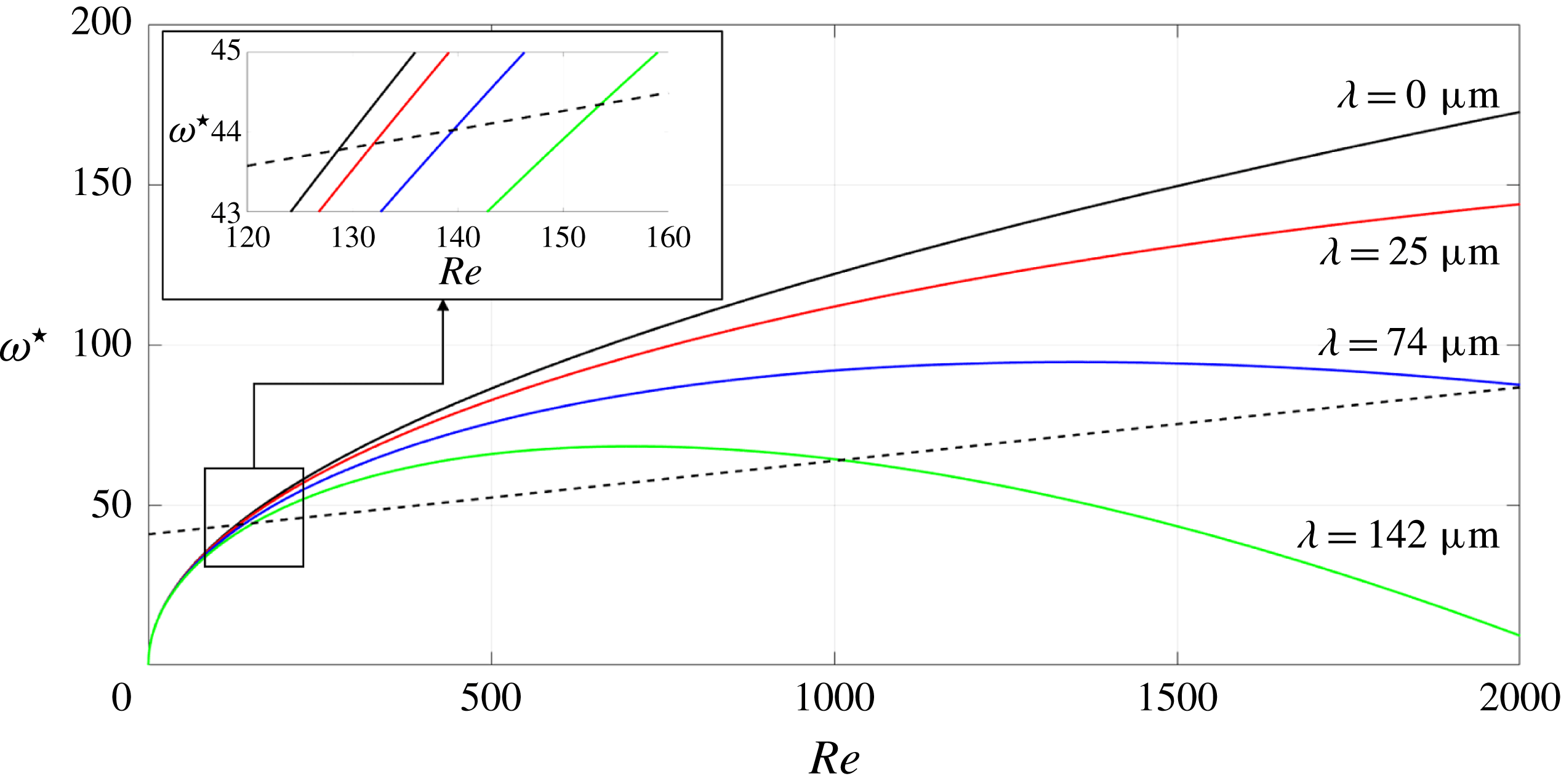
analysed in this work. The dashed line represents the limit between an axisymmetric and a non-axisymmetric wake behind the sphere that was proposed by Magnaudet & Mougin (Reference Magnaudet and Mougin2007) in their numerical study of wake instabilities of fixed three-dimensional bubbles. The main result of their criterion is the crucial importance of the amount of vorticity produced at the body surface and injected in the flow. Different boundary conditions at the body surface determine different amounts of vorticity. The law proposed by Magnaudet & Mougin (Reference Magnaudet and Mougin2007) is properly normalised in order to be comparable with our study. The Reynolds number field analysed in figure 20 approximately corresponds to the
 $Re_{\infty }$
range investigated by Magnaudet & Mougin (Reference Magnaudet and Mougin2007). The value
 $A=3.86$
in (3.1) was evaluated by forcing the no-slip curve to intersect the instability criterion curve at the Reynolds number where the first bifurcation of the sphere wake occurs (
 $Re_{\infty }=210$
or equivalently
 $Re=129$
). Interestingly, for large enough slip values the model predicts the amount of surface vorticity to go back below the line describing the first regular bifurcation. In this case, at large enough Reynolds number the vorticity flux advected downstream prevails over the vorticity generation at the surface: not enough vorticity is accumulated for the transition to occur (see e.g. Leal Reference Leal1989; Legendre et al.
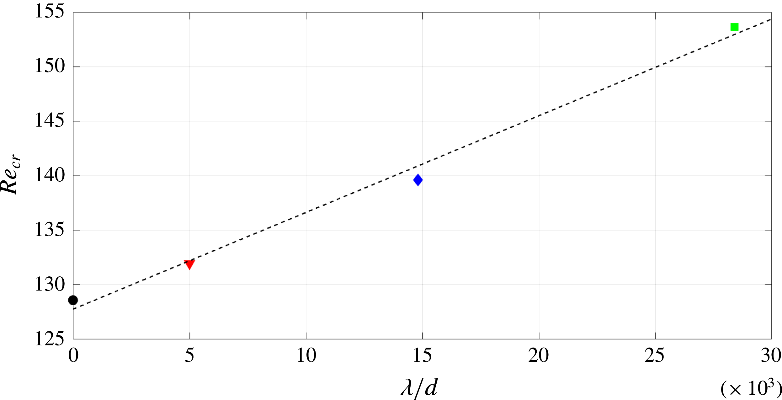
Reference Legendre, Lauga and Magnaudet2009). The inset in figure 20 shows a detail of the critical region: larger slip induces an increase of the critical Reynolds number
 $Re_{cr}$
at which the transition occurs. The linear relationship between
 $Re_{cr}$
and
 $\unicode[STIX]{x1D706}/d$
is reported in figure 21, where the slope of the fitting line is approximately equal to 0.9. The model thus predicts, under the hypothesis of an ideal non-deformable slip wall, a delay effect of slip on the transition occurrence. The conflict between the model assumptions and results and the experimental evidence are discussed in § 4.
Predicted vorticity at the surface of a sphere (see (3.1)) as a function of the Reynolds number. Solid black:
 $\unicode[STIX]{x1D706}=0~\unicode[STIX]{x03BC}\text{m}$
. Solid red:
 $\unicode[STIX]{x1D706}=25~\unicode[STIX]{x03BC}\text{m}$
. Solid blue:
 $\unicode[STIX]{x1D706}=74~\unicode[STIX]{x03BC}\text{m}$
. Solid green:
 $\unicode[STIX]{x1D706}=142~\unicode[STIX]{x03BC}\text{m}$
. The dashed line represents the critical curve between an axisymmetric standing eddy and a three-dimensional wake (see (4.1) in Magnaudet & Mougin (Reference Magnaudet and Mougin2007)). The inset shows the detail of the critical region.

Predicted critical Reynolds number (see (3.1)) as a function of the non-dimensional roughness. ●, Reference (smooth) sphere. ▾, SH-NAR coating. ♦, SH-220 coating. ▪, SH-80 coating. Dashed line: best fit of the data in the least-mean square sense.

Appendix C. Instantaneous forces evaluation
In this appendix, we provide some details about the strategy used to derive the instantaneous lift coefficient
 $C_{L}$
acting on the falling sphere. For full details, please refer to Mougin & Magnaudet (Reference Mougin and Magnaudet2002a
), Shew et al. (Reference Shew, Poncet and Pinton2006).
Mougin & Magnaudet (Reference Mougin and Magnaudet2002a
) showed how, starting from the Kirchhoff equations describing the motion of a rigid body in an inviscid, incompressible and unbounded fluid, it is possible (Howe Reference Howe1995) to extend them in order to consider a viscous, rotational flow at rest at infinity. The same authors then showed how the joint exploitation of the Kirchhoff and the Navier–Stokes equations can solve the coupled problem where the body movement modifies the surrounding flow and the latter determines the body trajectory. This formulation was later considered by Shew et al. (Reference Shew, Poncet and Pinton2006) to evaluate the forces acting on rising bubbles. The starting point was the measurement of their three-dimensional trajectories. The generalised Kirchhoff equations that govern the motion of a rigid body of mass
 $m$
, volume
 ${\mathcal{V}}$
, velocity
 $\boldsymbol{V}$
and rotation rate
 $\unicode[STIX]{x1D734}$
are:
 $$\begin{eqnarray}\displaystyle & \displaystyle (m\unicode[STIX]{x1D644}+\unicode[STIX]{x1D726})\frac{\text{d}\boldsymbol{V}}{\text{d}t}+\unicode[STIX]{x1D734}\times ((m\unicode[STIX]{x1D644}+\unicode[STIX]{x1D726})\boldsymbol{V})=\boldsymbol{F}+\boldsymbol{F}_{b}, & \displaystyle\end{eqnarray}$$
 $$\begin{eqnarray}\displaystyle & \displaystyle (\unicode[STIX]{x1D645}+\unicode[STIX]{x1D63F})\frac{\text{d}\unicode[STIX]{x1D734}}{\text{d}t}+\unicode[STIX]{x1D734}\times ((\unicode[STIX]{x1D645}+\unicode[STIX]{x1D63F})\unicode[STIX]{x1D734})+\boldsymbol{V}\times (\unicode[STIX]{x1D726}\boldsymbol{V})=\unicode[STIX]{x1D71E}, & \displaystyle\end{eqnarray}$$
where
 $\unicode[STIX]{x1D644}$
is the unity tensor,
 $\unicode[STIX]{x1D645}$
is the inertia tensor of the body,
 $\unicode[STIX]{x1D726}$
is the added mass tensor and
 $\unicode[STIX]{x1D63F}$
is the added rotational inertia tensor. On the right-hand side of the above equations
 $\boldsymbol{F}$
and
 $\unicode[STIX]{x1D71E}$
are the hydrodynamic forces (lift and drag) and torques respectively, and
 $\boldsymbol{F}_{b}$
is the gravity/buoyancy force. The chosen frame of reference rotates with the sphere (see figure 3(b) in Shew et al. (Reference Shew, Poncet and Pinton2006)): the 1-direction is parallel to the instantaneous sphere velocity vector, the 2-direction is perpendicular to the 1-direction so that the plane 1–2 is always vertical. The third direction is orthogonal to the 1–2 plane, and hence is always horizontal. The forces acting along the 1-direction are therefore the drag
 $D$
and the component of the gravity/buoyancy force
 $F_{b1}$
. Along the 2-direction act the components
 $L_{2}$
and
 $F_{b2}$
of the lift and gravity/buoyancy forces, respectively. Finally, only the component
 $L_{3}$
of the lift force acts along the 3-direction. In the considered reference system
 $\boldsymbol{V}=(V,0,0)$
and
 $\unicode[STIX]{x1D726}$
is time independent with a 1/2 coefficient on the diagonal due to the considered spherical geometry (see e.g. Magnaudet & Eames Reference Magnaudet and Eames2000). The point symmetry of the analysed geometry also simplifies the handling of the rotational degrees of freedom, which reduce to (Shew et al.
Reference Shew, Poncet and Pinton2006):
 $$\begin{eqnarray}\displaystyle & \displaystyle \unicode[STIX]{x1D6FA}_{1}=\frac{\text{d}\unicode[STIX]{x1D719}}{\text{d}t}\cos \unicode[STIX]{x1D703}, & \displaystyle\end{eqnarray}$$
 $$\begin{eqnarray}\displaystyle & \displaystyle \unicode[STIX]{x1D6FA}_{2}=\frac{\text{d}\unicode[STIX]{x1D719}}{\text{d}t}\sin \unicode[STIX]{x1D703}, & \displaystyle\end{eqnarray}$$
 $$\begin{eqnarray}\displaystyle & \displaystyle \unicode[STIX]{x1D6FA}_{3}=-\frac{\text{d}\unicode[STIX]{x1D703}}{\text{d}t}, & \displaystyle\end{eqnarray}$$
 $\unicode[STIX]{x1D703}$
is the pitch angle between
 $\boldsymbol{V}$
and the vertical direction, and
 $\unicode[STIX]{x1D719}$
is the azimuthal angle between the horizontal projection of the 1-direction and a fixed horizontal line. All the above assumptions reduce the problem to the following set of equations:
 $$\begin{eqnarray}\displaystyle & \displaystyle (m+\unicode[STIX]{x1D6EC}_{11})\frac{\text{d}V}{\text{d}t}=D+F_{b1}, & \displaystyle\end{eqnarray}$$
 $$\begin{eqnarray}\displaystyle & \displaystyle \unicode[STIX]{x1D6FA}_{3}(m+\unicode[STIX]{x1D6EC}_{11})V=L_{2}+F_{b2}, & \displaystyle\end{eqnarray}$$
 $$\begin{eqnarray}\displaystyle & \displaystyle -\unicode[STIX]{x1D6FA}_{2}(m+\unicode[STIX]{x1D6EC}_{11})V=L_{3}, & \displaystyle\end{eqnarray}$$
 $F_{b1}=(\unicode[STIX]{x1D70C}_{s}-\unicode[STIX]{x1D70C}_{f}){\mathcal{V}}g\cos \unicode[STIX]{x1D703}$
and
 $F_{b2}=(\unicode[STIX]{x1D70C}_{s}-\unicode[STIX]{x1D70C}_{f}){\mathcal{V}}g\sin \unicode[STIX]{x1D703}$
. The only unknowns in (C 4) are the instantaneous drag and lift magnitudes, since from the available three-dimensional sphere movement it is possible to evaluate
 $\unicode[STIX]{x1D703}=\arccos (V_{z}/V)$
and
 $\text{d}\unicode[STIX]{x1D719}/\text{d}t=(V_{x}\,\text{d}V_{y}/\text{d}t-V_{y}\,\text{d}V_{x}/\text{d}t)/V_{tr}^{2}$
, with the transversal velocity defined as
 $V_{tr}=\sqrt{V_{x}^{2}+V_{y}^{2}}$
, where the coordinate system (
 $x$
,
 $y$
,
 $z$
) was illustrated in figure 2. The knowledge of the instantaneous evolution of the velocity vector therefore allows for the calculation of the time evolution of the forces acting on the falling sphere. Notice that (C 4) predict a purely vertical falling when a zero lift force acts on the sphere, in agreement with the findings that link the transversal motion with the wake instabilities (see e.g. Mougin & Magnaudet Reference Mougin and Magnaudet2002a
). In that case, equations (C 4) reduce to (4.1) introduced in § 4.1.