1 Introduction
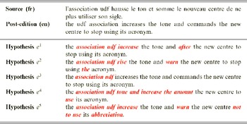
The core idea of Statistical Machine Translation (SMT) is to generate all possible hypotheses for a given input sentence, then search for the hypothesis of highest score to become the output. The score used to judge the candidates consists of various factors, e.g. language model (LM), translation model, reordering model, etc. Since the state-of-the-art MT models are imperfect, their outputs might not meet the user’s expectations. More specifically, the MT output perhaps beats the others under the decoder’s assessment, yet in many cases remains sub-optimal according to readers’ viewpoint. For instance, by looking at the N-best list presented in Table 1, it is not hard to realize that the third ranked hypothesis is more valuable than the current 1-best, with only one ‘Shift’ operation (‘association udf’ → ‘udf association’) is required to become the reference (post-edition), although its model score is lower.
With state-of-the-art SMT systems, the 1-best is not always optimal

Therefore, improving MT performance by adding more objective and decoder-independent features is a roadmap that many researchers are attempting. Joining these endeavors, this paper contributes two novel ideas for generating a better candidate from the quality labels predicted for words of the current MT output. More specifically, we automatically identify the good and bad words (word confidence estimation (WCE)), then exploit them as additional indicators to ‘decode’ one more time for acquiring more valuable translation. There are two spaces over which the search can be conducted:
-
• The MT N -best list: After decoding, besides the official translation e 1, the decoder generates also N − 1 other alternative hypotheses {e 2, e 3, . . ., eN } with lower scores. The totality of these N hypotheses is known as the N-best list. Working on this list, we integrate into the current objective scoring function with our proposed parameters based on WCE scores, then re-rank it by this enriched function.
-
• The MT search graph (SG) can be considered as a ‘vast warehouse’ storing all possible hypotheses generated by the SMT decoder. Our idea when exploring this huge space is that the overall scores of all paths containing tagged (error/no error) words will be modified due to their quality predicted beforehand by WCE. More precisely, the score is strengthened (increased) in case of the path contains good words and weakened (decreased) otherwise.
WCE is not a novel topic, although it is still under-studied compared to research on Sentence-level Quality Estimation. Nevertheless, the idea of using it to enhance MT quality has not been widely investigated in literature. To the best of our knowledge, if we ignore our previously published conference papers, the confidence score (called Goodness) is applied only once in the work of Nguyen, Huang and Al-Onaizan (Reference Nguyen, Huang and Al-Onaizan2011) to re-rank the N-best list, in a different way from our approach.
The rest of this paper is organized as follows. After reviewing some related work in Section 2, we investigate the correlation between our proposed scores (built using WCE) and other MT quality metrics (BLEU, TER, TERp-A) in Section 3. Section 4 presents the WCE system building. Sections 5 details the idea of using WCE to re-rank the N-best list. Another way of exploiting it to re-decode the SMT SG is discussed in Section 6. Section 7 compares the two methods, concludes the paper and points some perspectives.
2 Related work
2.1 Word confidence estimation
Confidence estimation is the task of identifying the correct parts and detecting the translation errors in MT output. If the quality is predicted for each word, this becomes WCE. The interesting uses of WCE include pointing out the words that need to be corrected by the post-editor, telling readers about the reliability of a specific portion, and selecting the best segments among options from multiple translation systems for combination.
To deal with this problem, various approaches have been proposed. They mainly focus on two principal issues: the features to represent each word and the Machine Learning methods to train the classifier. In this domain’s pioneer work, Blatz et al. (Reference Blatz, Fitzgerald, Foster, Gandrabur, Goutte, Kulesza, Sanchis and Ueffing2003) combine several features using neural network and Naïve Bayes learning algorithms. One of the most effective feature combinations is the Word Posterior Probability (WPP) as suggested by Ueffing, Macherey and Ney (Reference Ueffing, Macherey and Ney2003) associated with IBM-model-based features (Blatz et al. Reference Blatz, Fitzgerald, Foster, Gandrabur, Goutte, Kulesza, Sanchis and Ueffing2004). Basically, WPP is the likelihood of the word occurring in the target sentence, given the source sentence. Numerous knowledge sources have been proposed to calculate it, such as word graphs, N-best lists, etc. To quantify it, the key point is to determine sentences in N-best lists that contain the word e under consideration in a fixed position i.
Ueffing and Ney (Reference Ueffing and Ney2005) propose an approach for phrase-based translation models: A phrase is a sequence of contiguous words and is extracted from the word-aligned bilingual training corpus. The confidence value of each word is then computed by summing over all phrase pairs in which the target part contains this word. Xiong, Zhang and Li (Reference Xiong, Zhang and Li2010) incorporate linguistic features (the word itself, part-of-speech (POS) and null-link feature) with WPP and train their Maximum Entropy classifier, allowing considerable gains in comparison to the one using only WPP features. The novel features from source side, alignment context, and dependency structure (Nguyen et al. Reference Nguyen, Huang and Al-Onaizan2011) advance the error prediction accuracy of the baseline system using WPP and POS features in both F-score and Pearson correlation with human judgment. Other approaches are based on external features, which are independent from MT system’s resources (Soricut and Echihabi Reference Soricut and Echihabi2010; Felice and Specia Reference Felice and Specia2012), allowing to cope with various MT systems, such as statistical, rule-based, etc.
Recent workshops on MT (WMT 2013, 2014, and 2015) launched WCE as an evaluation shared task. In WMT 2013, while Han et al. (Reference Han, Lu, Wong, Chao, He and Xing2013), Luong, Lecouteux and Besacier (Reference Luong, Lecouteux and Besacier2013) employ the Conditional Random Fields model (Lafferty et al. Reference Lafferty, McCallum and Pereira2001) to build classifiers, Bicici (Reference Bicici2013) presents the global learning model by dynamic training with adaptive weight updates in the perceptron training algorithm. Concerning features: Bicici (Reference Bicici2013) presents the ‘common cover links’ (the links that point from the leaf node containing this word to other leaf nodes in the same subtree of the syntactic tree). Han et al. (Reference Han, Lu, Wong, Chao, He and Xing2013) focus on various n-gram combinations of target words. Luong et al. (Reference Luong, Lecouteux and Besacier2013) integrated a number of new indicators relying on graph topology, pseudo reference, syntactic behavior (constituent label, distance to the semantic tree root), and polysemy characteristic.
In WMT 2014, Wisniewski et al. (Reference Wisniewski, Pécheux, Allauzen and Yvon2014) exploit random forest classifier and build only 16 dense and continuous features of two categories: association features between source sentence and each target word, and fluency features describing the quality of the translation hypotheses. Meanwhile, confusion network, word lexicon, and POS tags are the main resources to form the feature set of the systems of Camargo-de-Souza et al. (Reference Camargo-de-Souza, González-Rubio, Buck, Turchi and Negri2014).
In WMT 2015, deep neural network is employed by Kreutzer, Schamoni and Riezler (Reference Kreutzer, Schamoni and Riezler2015) to learn continuous feature representations from bilingual contexts. Their network is firstly trained by initializing the word lookup-table with distributed word representation, and then adapted to the WCE task via a back-propagation process, which aims to minimize the word prediction errors using stochastic gradient descent. Meanwhile, the conventional sequence labeling technique, Conditional Random Fields, is applied by many other participants (Shah et al. Reference Shah, Logacheva, Paetzold, Blain, Beck, Bougares and Specia2015; Logacheva et al. Reference Logacheva, Hokamp and Specia2015; Shang et al. Reference Shang, Cai and Ji2015) to train their classifiers. Beside using baseline features, Tezcan et al. (Reference Tezcan, Hoste, Desmet and Macken2015) propose new ones to capture the accuracy (meaning transfer from source to target sentence) using word and phrase alignments, and the fluency (target sentence well-formedness level) via training LM on word surface forms and on POS tags.
As stated above, the main goal of this paper is to apply WCE outputs in the second pass of decoding (i.e. for re-ranking the SMT N-best list, as well as re-decoding the SG). Therefore, it is interesting to investigate how SMT multiple-pass decoding was examined in the literature in the next section.
2.2 SMT multiple-pass decoding
Among related work concerning this issue, we observe some prominent ideas. The first direction focuses on proposing additional LM. Kirchhoff and Yang (Reference Kirchhoff and Yang2005) train one word-based 4-gram model (with modified Kneser–Ney smoothing) and one factored trigram model, then combine them with seven decoder scores for re-ranking N-best lists of several SMT systems. Their proposed LMs increase the translation quality of the baselines (measured by BLEU score) from 21.6 to 22.0 (Finnish–English), or from 30.5 to 31.0 (Spanish–English). Meanwhile, Zhang, Almut and Stephan (Reference Zhang, Almut and Stephan2006) experiment with a distributed LM where each server, among the total of 150, hosts a portion of the data and responses its client, allowing them to exploit an extremely large corpus (2.7 billion word English Gigaword) for estimating N-gram probability. The quality of their Chinese–English hypotheses after the re-scoring process by using this LM is improved by 4.8 per cent (from BLEU 31.44 to 32.64, oracle BLEU score = 37.48).
In another direction, several authors propose to replace the current decoder’s linear scoring function by more efficient functions. Ueffing and Ney (Reference Ueffing and Ney2007) linearly combine sentence-level WPP with scores assigned by the underlying SMT system and additional LM scores. Sokolov, Wisniewski and Yvon (Reference Sokolov, Wisniewski and Yvon2012b) learn their non-linear scoring function in a learning-to-rank paradigm, applying Boosting algorithm. Their gains on the WMT’{10, 11, 12} are modest yet consistent and higher than those based on linear scoring functions. Duh and Kirchhoff (Reference Duh and Kirchhoff2008) use Minimum Error Rate Training (MERT) (Och Reference Och2003) as a weak learner and build their own solution, BoostedMERT, a highly expressive re-ranker created by voting among multiple MERT ones. Their proposed model considerably beats the decoder’s log-linear model (43.7 versus 42.0 BLEU) in IWSLT 2007 Arabic–English task. Aiming at lattice re-scoring methods for large-scale SMT, Blackwood (Reference Blackwood2010) proposes a linearized lattice minimum Bayes-risk decoding method based on efficient path counting transducers. He also suggests to combine multiple SMT lattices, allowing the decoder to operate on a much richer and more diverse searching space, thus improves the translation quality over several language pairs. Applying solely goodness (the sentence confidence) scores, Nguyen et al. (Reference Nguyen, Huang and Al-Onaizan2011) obtain slight yet consistent TER reductions (0.007 and 0.006 on the dev and test set) after a five-list re-ranking for their SMT hypotheses. This latter work is the most related to our paper, yet discrepant in some points: (1) our proposed sentence scores are computed based on word confidence labels; (2) we perform a study of the use of WCE for N-best reranking and assess its usefulness in a simulated interactive scenario (using oracle WCE labels); and (3) we also use, in the second part of this paper, the WCE score to re-decode the full SMT SG.
3 Word quality scores and MT quality metrics
Before exploiting WCE scores to improve MT quality, we first investigate the correlation between sentence-level scores (obtained from WCE labels) and conventional evaluation scores, including BLEU (Papineni et al. Reference Papineni, Roukos, Ard and Zhu2002), TER and TERp-A (Snover Reference Snover, Madnani, Dorr and Schwartz2008). For each output sentence, a word quality score is defined by the ratio of the number of words predicted as ‘Good’ by WCE system over its total number of words:
 $$\begin{equation}
WQS=\frac{\#^{\prime \prime }G^{\prime \prime } (good) \ words}{\#words}
\end{equation}$$
In other words, we are trying to examine whether the high percentage of ‘G’ (good) words (predicted by WCE system) in an MT output ensure its possibility of having a better BLEU and low TER (TERp-A) value. This investigation is a strong prerequisite for further experiments in order to verify that WCE scores do not bring additional ‘noise’ to the candidates’ re-judgement process. In this investigation, we compute word quality score over a French–English dataset (encompassing total of 10,881 1-best translations), taken from news corpora of the WMT evaluation campaign (from 2006 to 2010). The post-editions of these translations are generated by using a crowdsourcing platform: Amazon Mechanical Turk. Matching MT hypotheses against post-editions using TERp-A,Footnote 1 a tuned version of TERp,Footnote 2 enables us not only to compute TER and TERp-A scores, but also to determine the word quality labels (‘G’, ‘B’), and then word quality score. More details of the corpus can be found in Potet et al. (Reference Potet, Rodier, Besacier and Blanchon2012) and those of the quality label determination with TERp-A are depicted in Luong (Reference Luong2012). Once TERp-A labels are obtained, we convert them into binary labels ‘G’, ‘B’ (see Section 4.2 for conversion details). Once we have three conventional scores (BLEU, TER, TERp-A) for each sentence, we plot each against word quality score. Here, we use the ‘oracle’ labels in order to verify the correlation with conventional evaluation metrics, but obviously, the predicted labels will be used for the two-pass SMT described in the next section. BLEU, TER, and TERp-A scores are calculated after matching with post-editions. The results are plotted in Figure 1, where the y axis shows the ‘G’ (good) word percentage, and the x axis shows BLEU (1a), TER (1b), or TERp-A (1c) scores.
The correlation between WQS in a sentence and its overall quality measured by: (a) BLEU, (b) TER and (c) TERp-A metrics.

It can be seen from Figure 1 that the majority of points (the densest areas) in all three cases conform the common tendency. In Figure 1(a), the higher ‘G’ percentage, the higher BLEU score is. Conversely, in Figure 1(b) (Figure 1(c)), the higher ‘G’ percentage, the lower TER (TERp-A) is. Furthermore, these high correlations are quantified by the high positive (0.7814 for BLEU) and negative ( − 0.8687 for TER, and − 0.7968 for TERp-A) correlation scores. We notice some outliers, i.e. sentences with most or almost all words labeled ‘good’, yet still have low BLEU or high TER (TERp-A) scores. This phenomenon is to be expected when many unknown source words are not translated or when the unique reference is simply too far from the hypothesis. Nevertheless, the information extracted from oracle WCE labels seems useful to assess the MT hypotheses in the second pass.
4 Experimental setting
4.1 Dataset, N-best list, and search graph preparation
From a dataset of 10,881 French sentences, we applied a Moses-based SMT system to generate their English hypotheses. In our SMT system, the translation model is trained on the Europarl and News parallel corpora of WMT10Footnote 3 (1,638,440 sentences), and the target LM is trained by the SRILM toolkit (Stolcke Reference Stolcke2002) on a news monolingual corpus of WMT10 (48,653,884 sentences). Next, human translators were invited to correct MT outputs, giving us the post editions. More details on this post-edited corpus can be found in Potet et al. (Reference Potet, Rodier, Besacier and Blanchon2012). The set of triples (source, hypothesis, post edition) was then divided into the training set (10,000 first triples) and test set (881 remaining ones). The WCE classifier was trained over all one-best hypotheses of the training set.
The N-best list (N = 1, 000) with associated alignment information is also obtained on the test set (1,000 × 881 = 881,000 sentences) by using options ‘-n-best-list’ and ‘-print-alignment-info-in-n-best’ of Moses (version 2009-04-13) (Koehn et al. Reference Koehn, Hoang, Birch, Callison-Burch, Federico, Bertoldi, Cowan, Shen, Moran, Zens, Dyer, Bojar, Constantin and Herbst2007). Besides, the SGs are extracted by some parameter settings: ‘-output-search-graph’, ‘-search-algorithm 1’ (using cube pruning), and ‘-cube-pruning-pop-limit 5,000’ (adds 5,000 hypotheses to each stack). We then store the SG for each source sentence in a separated file, and the average size is 43.8 MB.
4.2 WCE system building
We employ the Conditional Random Fields (Lafferty et al. Reference Lafferty, McCallum and Pereira2001) as our machine learning method, with WAPITI toolkitFootnote 4 (Lavergne, Cappé and Yvon Reference Lavergne, Cappé and Yvon2010), to train the WCE model. A number of knowledge resources are employed for extracting the system-based, lexical, syntactic, and semantic characteristics of a word. This results in the total of 25 major feature types as follows:
-
• Target Side: target word; bigram (trigram) backward sequences; number of occurrences.
-
• Source Side: source word(s) aligned to the target word.
-
• Alignment Context (Nguyen et al. Reference Nguyen, Huang and Al-Onaizan2011): the combinations of the target (source) word and all aligned source (target) words in the window ± 2.
-
• WPP (Ueffing et al. Reference Ueffing, Macherey and Ney2003).
-
• Pseudo-reference (Google Translate): does the word appear in the pseudo reference?
-
• Graph topology (Luong, Besacier and Lecouteux Reference Luong, Besacier and Lecouteux2013): number of alternative paths in the confusion set, maximum and minimum values of posterior probability distribution.
-
• LM based: length of the longest sequence of the current word and its previous ones in the target (resp. source) LM. For example, with the target word wi : if the sequence w i − 2 w i − 1 wi appears in the target LM but the sequence w i − 3 w i − 2 w i − 1 wi does not, the n-gram value for wi will be 3.
-
• Lexical Features: word’s POS obtained by TreeTagger toolkitFootnote 5 on both source and target sides; sequence of POS of all its aligned source words; POS bigram (trigram) backward sequences; binary lexical features: is the character sequence a punctuation? a proper name? a numerical value?
-
• Syntactic Features: null link (Xiong et al. Reference Xiong, Zhang and Li2010); constituent label; depth in the constituent tree.
-
• Semantic Features: number of word senses in WordNet.
In the next step, the word’s reference labels (or so-called oracle labels) are initially set by using TERp-A toolkit (Snover Reference Snover, Madnani, Dorr and Schwartz2008) in one of the following classes: ‘I’ (insertions), ‘S’ (substitutions), ‘T’ (stem matches), ‘Y’ (synonym matches), ‘P’ (phrasal substitutions), ‘E’ (exact matches). ‘E’, ‘T’, and ‘Y’ are then regrouped into ‘good’ class ‘G’, meanwhile the rest (‘I’, ‘P’, and ‘S’) belongs to ‘bad’ class ‘B’. We observe that eighty-five per cent of the words in our dataset are labeled as “G” and fifteen per cent are labeled as “B”. Once having the prediction model, we apply it on the test set (881 × 1,000 best = 881,000 sentences) and get needed WCE labels along with confidence probabilities. In terms of F-score, our WCE system gets performance in predicting ‘G’ label of 87.65 per cent, and‘B’ label of 42.29 per cent. The above-mentioned feature types were also used in our English–Spanish WCE System submitted for WMT Quality Estimation shared task and achieved a high rank (first rank in 2013 (Luong et al. Reference Luong, Lecouteux and Besacier2013) and third rank in 2014 (Luong, Besacier and Lecouteux (Reference Luong, Besacier and Lecouteux2014)). Both WCE and oracle labels will be used in the experiments.
5 WCE in N-best list re-ranking
As stated above, the main goal of this idea is to add WCE-based scores along with existing decoder ones (LM, Translation model, Reordering model, etc.) in order to re-select the best hypothesis among N candidates. We start by describing our proposed features, followed by experiments and further analysis.
5.1 Proposed features
Since the scores resulting from the WCE system are for words, we have to synthesize them in sentence level scores for integrating with the 14 (already existing) Moses decoder scores. Six new scores are proposed; they include the following:
-
• The ratio of number of good words to total number of words (1 score).
-
• The ratio of number of good nouns (verbs) to total number of nouns (verbs) (2 scores).
-
• The ratio of number of n consecutive good word sequences to the total number of consecutive word sequences; n = 2, n = 3, and n = 4 (3 scores).
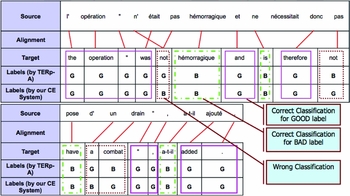
Let us give an example in Figure 2: Among the total of eighteen words of a given SMT hypothesis, we have twelve labeled as ‘G’; seven out of seventeen word pairs (bigram) are labeled as ‘GG’ and three out of sixteen triples are labeled as ‘GGG’. In this case, some of the above scores can be computed as
 $$\begin{eqnarray}
\frac{\#good \ words}{\#words} \ = \ \frac{12}{18} \ = 0.667 \nonumber \\
\frac{\#good \ bigrams}{\#bigrams} \ = \ \frac{7}{17} \ = 0.4118\\
\nonumber \frac{\#good \ trigrams}{\#trigrams} \ = \ \frac{3}{16} \ = 0.1875.
\end{eqnarray}$$
Example of our WCE classification results for one MT hypothesis.

With the features built on oracle labels, we are able to analyze the upper bound performance. In other words, we can establish an ‘oracle’ setting which is comparable to an interactive case where users would validate a word as ‘G’ or ‘B’ without providing any confidence score.
5.2 Experiments
To better examine the impact of the proposed scores, we calculate them not only using our predicted WCE system, but also using an oracle WCE (further called ‘WCE scores’ and ‘oracle scores’, respectively). We experiment with the three following systems:
-
• BL: Baseline SMT system with fourteen above decoder scores.
-
• BL+WCE: Baseline + 6 predicted WCE scores.
-
• BL+OR: Baseline + 6 oracle WCE scores (simulating an interactive scenario).
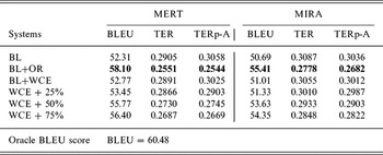
The weights assigned to these scores are tuned by a two-fold cross validation on the test set, using MERT (Och Reference Och2003) and MIRA (Watanabe et al. Reference Watanabe, Tsukada and Isozaki2007) methods. More specifically, we split the test set into two equivalent parts: S1 and S2, then take S1 as a development set to optimize the parameters which are then used to decode and re-rank the translations of S2, and vice versa. The translation quality of BL, BL+WCE, and BL+OR systems are reported in Table 2.
Translation quality of the baseline system (only decoder scores) and that with additional scores from real ‘WCE’ or ‘oracle’ WCE system

The results obtained show that the integration of oracle scores significantly boosts the MT output quality, measured by all three metrics and optimized by both tuning methods employed. We gained 5.79 and 4.72 points in BLEU score, by MERT and MIRA (respectively). With TER, BL+OR helps to gain 0.03 point in both methods. Meanwhile, in case of TERp-A, the improvement is 0.05 point for MERT and 0.03 point for MIRA. It is worthy to mention that the possibility of obtaining such oracle labels is doable through a human-interaction scenario (which could be built from a tool like Post-Editing Tool (Aziz, De Sousa and Specia Reference Aziz, De Sousa and Specia2012) for instance). In such an environment, once having the hypothesis produced by the first pass (translation task) , the human editor could simply click on words considered as bad (B), the other words being implicitly considered as correct (G).
For more insightful understanding about WCE scores’ role, we calculate the possible optimal BLEU score obtained from the N-best list. Applying the sentence-level BLEU+1 metric (Nakov, Guzman and Vogel Reference Nakov, Guzman and Vogel2012) over candidates in the list, we select the one with highest score and aggregate all of them in an oracle-best translation; the resulting performance obtained is 60.48. This score shows that the simulated interactive scenario (BL+OR) is less than optimal only 2.38 points (in case of MERT) and clearly overpasses the baseline (8.17 points below the best score).
The contribution of a real (predicted) WCE system seems more modest: BL+WCE marginally increases BLEU scores of BL (0.46 gain in case of optimizing by MERT and 0.32 by MIRA). For both TER and TERp-A metric, the improvements are also negligible. To verify the significance of this result, we estimate the p-value between BLEU of BL+WCE system and BLEU of baseline BL relying on Approximate Randomization method (Clark et al. Reference Clark, Dyer, Lavie and Smith2011) which indicates if the improvement yielded by the optimized system is likely to be generated again by some random processes (randomized optimizers). After various optimizer runs, we randomly selected five optimizer outputs to perform the Approximate Randomization test and obtain a p-value of 0.01. This result reveals that the improvement yielded by BL+WCE is significant although small, originated from the contribution of WCE score, not by any optimizer variance. This modest but positive change in BLEU score using WCE features encourages us to investigate and analyze further about WCE scores’ impact by illustrating the gradual improvement of WCE performance, which we now explain. First, we filter out all wrongly classified words in the test set (by matching against the oracle labels) and push them into a temporary set, called T. Then, we correct randomly a percentage (twenty-five per cent, fifty per cent, or seventy-five per cent) of labels in T. Finally, the altered T will be integrated back with the correctly predicted part (by the WCE system) in order to form a new ‘simulated’ result set. This strategy results in three ‘virtual’ WCE systems called ‘WCE+N%’ (N = 25, 50, or 75), which use fourteen decoder scores (including seven reordering, one LM, five translation model, and one word penalty scores), and six ‘simulated’ WCE scores. From each of the above systems, the whole experimental setting is identical to what we did with the original WCE and oracle systems: six scores are built and combined with existing fourteen system scores for each hypothesis in the N-best list. After that, MERT and MIRA methods are invoked to optimize their weights, and finally the reordering is performed thanks to these scores and appropriate optimal weights. The translation quality measured by BLEU, TER, and TERp-A after re-ranking using ‘WCE+N%’ (N = 25,50,75) can be seen also in Table 2.
We note that all obtained scores behave as expected: the better performance WCE system reaches, the clearer its role in improving MT output quality. Diminishing twenty-five per cent of the wrongly predicted words leads to a gain of 0.68 point (by MERT) and 0.32 (by MIRA) in BLEU score. More significant increases of BLEU 3.00 and BLEU 3.63 (MERT) can be achieved when prediction errors decrease up to fifty per cent and seventy-five per cent. These scores suggest that WCE has a promising role in improving MT quality if its quality is adequate.
6 WCE for SMT search graph re-decoding
The major drawback of the approach previously presented is that the search is limited to a set of N best sentences. What would happen if this space was widened? Will it be efficient for mining better hypothesis? These questions motivate us to investigate SMT SG re-decoding.
6.1 Search graph structure
The SMT decoder’s SG can be roughly considered as a ‘vast warehouse’ storing most promising hypotheses generated by the SMT system during decoding for a given source sentence. In this large directed acyclic graph, each hypothesis is represented by a path, carrying all nodes between its start and end ones, along with the edges connecting adjacent nodes. One hypothesis is called complete when all the source words are covered and incomplete otherwise. Starting from the empty initial node, the SG is gradually enlarged by expanding hypotheses during decoding. In order to facilitate the access and the cost calculation, each hypothesis H is further characterized by the following fields:
-
• hyp: hypothesis ID.
-
• back: the backpointer pointing to its previous cheapest path.
-
• transition: the cost to expand from the previous hypothesis (denoted by pre(H)) to this one.
-
• score: the cost of this hypothesis: score(H) = score(pre(H)) + transition.
-
• out: the last output (target) phrase, can contain multiple words.
-
• covered: the source coverage of out, represented by the start and the end position of the source words translated into out.
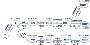
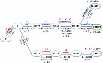
Figure 3 illustrates a simple SG generated for the source sentence: ‘identifier et mesurer les facteurs de mobilization’ . The attributes ‘t’ and ‘c’ refer to the transition cost and the source coverage, respectively. Hypothesis 175541 is extended from 57552, when the three words from third to fifth position of the source sentence (les facteurs de) are translated into ‘the factors of’ with the transition cost of − 8.5746. Hence, its cost is score(175541) = score(57552) + transition(175541) = −16.1014 + ( − 8.5746) = −24.6760. Three rightmost hypotheses: 204119, 204109, and 198721 are complete since they cover all source words. Among them, the cheapest-cost one is 198721, from which the model-best translation is read off by tracing back to the initial node 0: ‘identify the causes of action’ .
An example of search graph representation.

6.2 Overview of the approach
We assume that the decoder generates N best hypotheses T = {T 1, T 2, …, TN } at the end of the first pass. Using the WCE system (which can only be applied to sequences of words – and not directly to the SG – that is why N best hypotheses are used), we are able to assign the jth word in the hypothesis Ti , denoted by tij , with one appropriate quality label, cij (i.e. ‘G’ (Good: no translation error), ‘B’ (Bad: need to be edited)), along with the confidence probabilities (Pij (G), Pij (B) or P(G), P(B) for short, where P(B) = 1 − P(G)). Then, the second pass is carried out by considering every word tij as well as its labels and scores cij , P(G), P(B). Our principal idea is that, if tij is a positive (good) translation, i.e. cij = `G’ or P(G) ≈ 1, all hypotheses Hk ∈ SG containing it in the SG should be ‘rewarded’ by reducing their cost. On the contrary, those containing negative (bad) translation will be ‘penalized’. Let reward(tij ) and penalty(tij ) denote the reward or penalty score of tij . The new transition cost of Hk after being updated is formally defined by
 $$\begin{eqnarray}
transition^{\prime }(H_{k}) = transition(H_{k}) + \left\lbrace \begin{array}{@{}l@{\quad }l@{}}reward(t_{ij}) &\mbox{if}\quad t_{ij} = good\\
penalty(t_{ij}) &\mbox{if} \quad otherwise \end{array}\right.
\end{eqnarray}$$
The update finishes when all words in the N-best list have been considered. We then re-compute the new score of complete hypotheses by tracing backward via back-pointers and aggregating the transition cost of all their edges. Essentially, the re-decoding pass reorders SG hypotheses: the more ‘G’ words (predicted by WCE system) they contain, the more cost reduction will be made and consequently, the more opportunity they get to be the best hypothesis. It is vital to note that, during the update process, we might face a phenomena that the word tij (corresponds to the same source words) occurs in different sentences of the N-best list. In this case, for the sake of simplicity, we process it only at its first occurrence (in the highest rank sentence) instead of updating the hypotheses containing it multiple times. In other words, if we meet the word tij which aligns to the same source word once again in the next N-best sentence(s), no further score update will be done in the SG.
6.3 Update score definitions
Defining the update scores is a non-trivial issue as there is no quantitative estimate on the importance of WCE scores over the SG scores or vice versa. Our approach is to measure their importance empirically via weight optimization. In this paper, we propose several types of update scores, deriving from the global or local cost.
6.3.1 Definition #1: global update score
In this type, an unique score derived from the cost of the current best hypothesis H* (by the first pass) is used for all updates. We propose to compute this score by two ways: (a) exploiting WCE labels {cij }; or (b) only WCE confidence probabilities {P(G), P(B)} will matter and WCE labels will be left aside.
Definition #1a:
 $$\begin{eqnarray}
penalty(t_{ij}) = \alpha *\frac{score(H^{*})}{\#words(H^{*})}\\
reward(t_{ij}) = -penalty(t_{ij}) \nonumber
\end{eqnarray}$$
Where #words(H*) is the number of target words in H*, the positive coefficient α accounts for the impact level of this score on the final cost of the hypothesis and can be optimized during experiments. Here, penalty(tij ) gets negative sign (since score(H*) < 0) and will be added to the transition cost of all hypotheses containing tij in case where this word is labeled as ‘B’; whereas reward(tij ) (same value, opposite sign) is used in the other case.
Definition #1b:
 $$\begin{eqnarray}
update(t_{ij}) = \alpha *P(B)*\frac{score(H^{*})}{\#words(H^{*})} - \beta *P(G)*\frac{score(H^{*})}{\#words(H^{*})} \\
\nonumber = (\alpha *P(B) - \beta *P(G))*\frac{score(H^{*})}{\#words(H^{*})}
\end{eqnarray}$$
Where P(G), P(B) (P(G) + P(B) = 1) are the probabilities of ‘Good’ and ‘Bad’ class of tij
. The positive coefficients α and β can be tuned in the optimization phase. In this definition, the fact that update(tij
) is a reward (reward(tij
)) or a penalty (penalty(tij
)) will depend on tij
’s goodness. Indeed, we have update(tij
) = reward(tij
) if update(tij
) > 0, which means: α*[1 − P(G)] − β*P(G) < 0 (since score(H*) < 0), therefore
 $ P(G) > \frac{\alpha }{\alpha +\beta }$
.
On the contrary, if P(G) is under this threshold, update(tij ) takes a negative value and therefore becomes a penalty.
6.3.2 Definition #2: local update score
The update score of each (local) hypothesis Hk depends on its current transition cost, even when they cover the same word tij . Similarly to Definition 1, two sub-types are defined as follows:
Definition #2a:
 $$\begin{equation}
penalty(t_{ij}) = -reward(t_{ij}) = \alpha *transition(H_{k})
\end{equation}$$
Definition #2b:
 $$\begin{eqnarray}
update(t_{ij}) = \alpha *P(B)*transition(H_{k}) - \beta *P(G)*transition(H_{k})\nonumber \\
= (\alpha *P(B) - \beta *P(G))*transition(H_{k})
\end{eqnarray}$$
Where transition(Hk ) denotes the current transition cost of hypothesis Hk , and the meanings of coefficient α (Definition 2a) or α, β (Definition 2b) are analogous to those of Definition 1a (Definition 1b), respectively.
6.4 Re-decoding algorithm
Using WCE labels in SG decoding

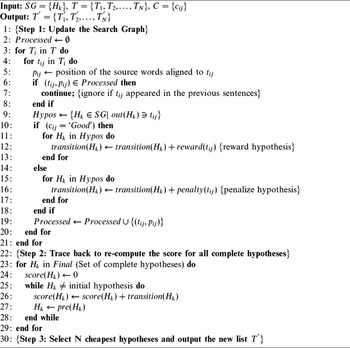
The above pseudo-code depicts our re-decoding algorithm using WCE labels. (Definition 1a and Definition 2a). The algorithm in case of using WCE confidence probabilities (Definition 1b and Definition 2b) is essentially similar, except the update step (from line 10 to line 18) is replaced by the following part:

During the update process, the pairs including the visited word tij and the position of its aligned source words pij are consequently admitted to be Processed, so that all the analogous pairs (t ′ ij , pij ′) occurring in the latter sentences can be discarded. For each tij , we search for all hypotheses in the SG whose the output phrase (stored in the field out) contains tij to form the set Hypo. To avoid the ambiguity where tij occurs multiple times in the sentence, the position coverage (stored in the field covered) must be ensured to bound the position of the aligned source word of the current tij . Then, the confidence score of tij , denoted by cij (or P(G)), determines whether all members Hk in Hypo will be rewarded or penalized. Once having all words in the N-best list visited, we obtain a new SG with updated transition costs for all edges containing them. On this updated SG, we re-compute the score of all complete hypotheses stored in Final. Finally, we backtrack the cheapest cost hypothesis to obtain the new translation.
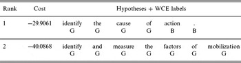
These above depictions can be clarified by taking another look at the example in Figure 3: From this SG, the N-best list (for the sake of simplicity, we choose N = 2) is generated as the single-pass decoder’s result. According to our approach, the second pass starts by tagging all words in the list with their confidence labels, as seen in Table 3. Then, the graph update process is performed for each word in the list, sentence by sentence, which details are tracked in Figure 4. In this example, we apply Definition 1a to calculate the reward or penalty score, with
 $\alpha = \frac{1}{2}$
, resulting in
 $penalty(t_{ij}) = -reward(t_{ij}) = \frac{1}{2}*\frac{-29.9061}{6} = -2.4922$
. First, all hypotheses containing words in the first ranked sentence are considered. Since the word ‘identify’ is labeled as ‘G’, its corresponding edge (connecting two nodes 0 and 1) is rewarded tnew
= told
+ reward = −1.8411 + 2.4922 = +0.6511. On the contrary, the edge between two nodes 121252 and 182453 is penalized and takes new cost: tnew
= told
+ penalty = −5.8272 + ( − 2.4922) = −8.3194, due to the bad quality of the word ‘action’. The edges having multiple considered words (e.g. between nodes 19322 and 121252) will be updated multiple times, and the transition costs after each update can be also observed in Figure 4 ( e.g. t1, t2, etc). Next, when the second best is taken into consideration, all repeated words (e.g. ‘identify’, ‘the’, and ‘of’) are ignored since they have been visited before, whereas the remaining ones are identically processed. The only untouched edge in this SG corresponds to the word ‘mobilizing’, as this word does not belong to the list. Once having the update process finished, we recalculate the final cost for every complete path and return the new best translation:
‘identify and measure the factors of mobilization’
(new cost = − 22.6414).
Details of update process for the SG in Figure 3. The first loop is represented in red color, while the second one is in blue. For edges with multiple updates, all transition costs after each update are logged. The winning cost is emphasized by green color.

The N-best (N = 2) list generated by the SG in Figure 3 and WCE labels

6.5 Experimented decoders
As in the re-ranking approach, we investigate the WCE’s contributions in two scenarios: predicted WCE and ideal WCE (oracles). We experiment with the seven following decoders:
-
• BL: Baseline (one-pass decoder).
-
• BL+WCE(1a, 1b, 2a, 2b): four two-pass decoders, using our estimated WCE labels and confidence probabilities to update the SGs, and the update scores are calculated by Definition (1a, 1b, 2a, 2b).
-
• BL+OR(1a, 2a): two two-pass decoders, computing the reward or penalty scores by Definition (1a, 2a) on the oracle labels.
It is important to note that, when using oracle labels, Definition 1b becomes Definition 1a and Definition 2b becomes Definition 2a, since if a word tij is labeled as ‘G’, then P(G) = 1 and P(B) = 0, and vice versa. In order to tune the coefficients α and β, we carry out a two-fold cross validation on the test set. First, the set is split into two equivalent parts: S1 and S2. Playing the role of a development set, S1 will train the parameters which are then used to compute the update scores on S2 re-decoding process, and vice versa. The optimization steps are handled by CONDOR toolkit (Frank Reference Frank2004), in which we vary α and β within the interval [0.00; 5.00]. Test set is further divided to launch experiments in parallel on our cluster using an open-source batch scheduler: OAR (Capit and Joseph Reference Capit and Joseph2013). This mitigates the overall processing times on such huge SGs. The re-decoding results for them are properly concatenated for evaluation. Tuned values for these parameters are: α = 0.9 (Definition 1a); α = 1.7, β = 0.8 (Definition 1b); α = 0.9 (Definition 2a); and α = 1.8, β = 0.8 (Definition 2b).
7 Results
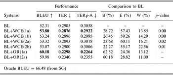
Table 4 shows the translation performances of all experimental decoders and their percentages of sentences which outperform, remain equivalent or degrade the baseline hypotheses (when match against the references, measured by TER). Results suggest that using oracle labels to re-direct the graph searching considerably boosts the baseline quality. BL+OR(1a) augments 7.87 points in BLEU, and diminishes 0.0607 (0.0794) point in TER (TERp-A), compared to BL. Meanwhile, with BL+OR(2a), these gains are 7.67, 0.0565, and 0.0514 (in that order). Besides, the contribution of our WCE system scores seems less prominent, yet positive: the best performing BL+WCE(1a) increases 1.49 BLEU points of BL (0.0029 and 0.0136 gained for TER and TERp-A). The small p -values (in the range [0.00; 0.02], seen on Table 2) estimated between BLEU of each BL+WCE system and that of BL using Approximate Method (Clark et al. Reference Clark, Dyer, Lavie and Smith2011) indicate that these performance improvements are significant. Results also reveal that the use of WCE labels is slightly more beneficial than that of confidence probabilities: BL+WCE(1a) and BL+WCE(2a) outperform BL+WCE(1b) and BL+WCE(2b). In both scenarios, we observe that the global update score (Definition 1) performs better compared to the local one (Definition 2). For more insightful understanding about WCE scores’ usefulness, we make a comparison with the best achievable hypotheses in the SG (oracles), based on the ‘LM Oracle’ approximation approach presented in Sokolov, Wisniewski and Yvon (Reference Sokolov, Wisniewski and Yvon2012a). This method simplifies the oracle decoding to the problem of searching for the cheapest path on a SG where all transition costs are replaced by the n-gram LM scores of the corresponding words. The LM is built for each source sentence uniquely using its target post-edition. We update the SG by assigning all edges with the LM back-off score of the word it contains. Finally, we combine the oracles of all sentences yielding BLEU oracle of 66.48: 6.30 points higher than BL+OR(1a). This result reveals that the use of oracle WCE scores, although helps to outperform significantly over the Baseline (52.31 BLEU → 60.18 BLEU), yet still remains a big gap to the best-achievable performance by SG re-decoding. It opens a room for future work on how to exploit WCE scores more efficiently toward this goal.
Translation quality of the conventional decoder and the two-pass decoders using scores from predicted or oracle WCE, followed by the percentage of better (B), equivalent (E) or worse (W) sentences compared to BL system, as well as p-values

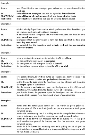
We close this section with some examples of outputs before and after the re-decoding process (shown in Table 5). In the first example, re-decoding yields a slightly better translation compared to the baseline MT system. Using labels predicted by WCE: ‘Bad’ for ‘a’ (at the beginning of the MT hypothesis) and ‘penalty’, and ‘Good’ for the rest, BL+WCE(1a) led to a new candidate whose last words (demoralization death) are closer to the post-edition (deadly demoralization) than the corresponding part of BL (penalty demoralisation). Similarly, in the second example, thanks to word error detection in the second example (tagged for ‘it has’, ‘speech that was’, and ‘post route’), BL+OR(1a) helped to translate correctly the pronoun (‘he’ instead of ‘it’), as well as to translate better the final part of the source sentence (into ‘after operating were normal’). The positive contributions of WCE-predicted labels and scores can also be observed in the remaining (from the third to the fifth) examples in the same table.
Examples of MT outputs before and after re-decoding

8 Discussion, conclusion, and perspectives
If we compare the performances between the use of WCE for N-best list re-ranking (Table 2) and SG Re-decoding (Table 4), the results suggest that the contribution of WCE in SG re-decoding outperforms that in N-best re-ranking in both ‘oracle’ or real scenarios. BL+OR(1a) outperforms its corresponding oracle re-ranker BL+OR( N -best_Reranking) in 2.08 points of BLEU, diminishes 0.0253 (0.0280) in TER (TERp-A). Meanwhile, BL+WCE(1a) beats BL+WCE( N -best_Reranking) (the re-ranker which uses predicted WCE scores) in 1.03 (BLEU), 0.0015 (TER), 0.0103 (TERp-A). In addition, there are 178 out of 881 sentences (20.20 per cent) outputted by BL+WCE(1a) that do not belong to the N-best list, suggesting that the re-decoding method can help to generate candidates which have not been nominated by SMT decoder. More notably, among these newly produced translations, 113 (63.5 per cent) translations are better than the corresponding one-best of the N-best list, measured by sentence-level BLEU+1 metric (Nakov et al. Reference Nakov, Guzman and Vogel2012). These positive results can be explained by the following facts: (1) in re-ranking, WCE scores are integrated at sentence level, so word translation errors are not fully penalized; and (2) in re-ranking, best translation selection is limited to the N-best list, whereas in re-decoding, we allow the search over the entire updated SG (on which not only N-best list paths but also those containing at least one word in this list are altered).
To conclude, we have presented two novel two-pass decoding methods for enhancing SMT quality. From the output of the first pass (N-best list), we predict words’ labels and confidence probabilities, then employ them to seek a more valuable candidate; first among the other in the N-best list, and then over the entire SGs. In both methods, while ‘oracle’ WCE labels substantially improve the MT quality (to reach the oracle score), real WCE achieves also the positive and promising gains. These methods show that error prediction using WCE helps to guide the decoding to less erroneous parts of the graph.
As future work, we plan to focus on enhancing our WCE system using more linguistic features as well as advanced techniques (feature selection, Boosting method. . .). We also focus on breaking down the translation errors (i.e.‘Bad’ label) into more concrete categories, so that they will be more informative. Besides, the update scores used in this paper will be further considered toward the consistency with SMT graph scores to obtain a better updated SG. Also, currently in the graph-re-decoding process, our WCE scores can only be applied to sequences of words – and not directly to the SG. Applying WCE to tag directly the SG will be part of future work. Finally, we will investigate the use of WCE labels to re-decode speech translation graphs and improve spoken language translation performance.