1 Introduction
Particles in fluid flows are ubiquitous (Toschi & Bodenschatz Reference Toschi and Bodenschatz2009), examples including plankton in the ocean (Ardekani et al. Reference Ardekani, Sardina, Brandt, Karp-Boss, Bearon and Variano2016; Guseva et al. Reference Guseva, Daitche, Feudel and Tél2016), colloidal spheres in Stokes flow, droplets in clouds (Falkovich, Fouxon & Stepanov Reference Falkovich, Fouxon and Stepanov2002; Govindarajan & Ravichandran Reference Govindarajan and Ravichandran2017; Ravichandran & Govindarajan Reference Ravichandran and Govindarajan2017), suspended particulate matter in the atmosphere and various industrial flows. The simplest way to study these flows is to assume a one-way interaction, where the particle dynamics is dictated by the flow, but does not disturb the flow, nor is it influenced by other particles. This is a good assumption when particles are far smaller than all relevant flow length scales, and when the suspension of particles is dilute, as is the case in several of the examples given above. In this setting, the particle obeys the Maxey–Riley (MR) equation (Maxey & Riley Reference Maxey and Riley1983), which is a force balance in Lagrangian coordinates, given by
 $$\begin{eqnarray}\displaystyle & \displaystyle \dot{\boldsymbol{y}}=\boldsymbol{v}(t), & \displaystyle\end{eqnarray}$$
 $$\begin{eqnarray}\displaystyle & \displaystyle R\dot{\boldsymbol{v}}=\frac{\text{D}\boldsymbol{u}}{\text{D}t}-\frac{1}{S}(\boldsymbol{v}-\boldsymbol{u})-\sqrt{\frac{3}{\unicode[STIX]{x03C0}S}}\left\{\frac{1}{\sqrt{t}}(\boldsymbol{v}(0)-\boldsymbol{u}(0))+\int _{0}^{t}\frac{\dot{\boldsymbol{v}}(s)-\dot{\boldsymbol{u}}(s)}{\sqrt{t-s}}\,\text{d}s\right\}, & \displaystyle\end{eqnarray}$$
 $$\begin{eqnarray}\displaystyle \unicode[STIX]{x1D6FD}\equiv \frac{\unicode[STIX]{x1D71A}_{p}}{\unicode[STIX]{x1D71A}_{f}},\quad S\equiv \frac{1}{3}\frac{a^{2}/\unicode[STIX]{x1D708}}{T},\quad R\equiv \frac{1+2\unicode[STIX]{x1D6FD}}{3}, & & \displaystyle\end{eqnarray}$$
where
 $\boldsymbol{y}$
and
 $\boldsymbol{v}$
are the vector position and velocity, respectively, of the particle, and
 $\boldsymbol{u}$
represents the (possibly spatially and temporally dependent) fluid velocity. We note here that, when spatial variation in the fluid is not accounted for in (1.2), the equation is known as the Basset–Boussinesq–Oseen equation (Clift, Grace & Weber Reference Clift, Grace and Weber2005; Parmar et al.
Reference Parmar, Annamalai, Balachandar and Prosperetti2018). As our focus is towards general fluid flows, we stick to the nomenclature of Maxey–Riley equation. Dots represent Lagrangian derivatives in time
 $t$
and
 $\text{D}/\text{D}t$
represents the material derivative with respect to the fluid velocity. Furthermore
 $\unicode[STIX]{x1D71A}_{p}$
and
 $\unicode[STIX]{x1D71A}_{f}$
are the particle and fluid density, respectively,
 $R$
is the effective density ratio including added-mass effects, and
 $S$
is the Stokes number, defined here as the ratio of particle relaxation time scale to flow time scale. The last term on the right-hand side of (1.2) is known as the Basset history force or Basset history integral (Basset Reference Basset1888). It is an integral force along the trajectory of the particle, from the initial time until time
 $t$
, resulting from the differences in acceleration of particle and surrounding fluid, and will be of primary interest in this paper. An important contribution to the force balance was brought out by Farazmand & Haller (Reference Farazmand and Haller2015), who showed the existence of a singular contribution from a non-zero relative velocity at the initial time instant. Thus far in the literature, the implications of this singular term are largely unexplored. We will discuss its significance in later sections.
Situations for which analytical solutions including the Basset force are provided by the present approach: (a) relaxing particle, (b) particle settling under gravity, (c) particle in an oscillating field, (d) particle in a shear flow, and (e) particle in a single point vortex.

Most studies concerning particle dynamics in the low-Stokes-number limit include contributions from the Stokes drag, the second term on the right-hand side in (1.2), but the Basset history integral is often neglected. The coefficient of this term is
 $O(S^{1/2})$
relative to the Stokes drag, so it is nominally negligible at small Stokes number, but the factor it multiplies could cause the effect to become important in physical flows. A major hurdle in evaluating the Basset history integral is the continually increasing memory cost associated in computing this term. The inclusion of the Basset history integral renders the MR equations to not represent a dynamical system, i.e. the future evolution of the particle motion depends not only on the current position and velocity, but also on the entire solution up to that time. Standard analytical techniques such as performing a Laplace transform are in general not useful in solving this fully nonlinear equation. Moreover, even for the linear case, inverting the Laplace transform of a general function
 $G(t)$
with a kernel of the form
 ${\sim}1/\sqrt{t}$
multiplying it does not lead to an explicit function of
 $t$
. Thus researchers have resorted to quadrature schemes (Van Hinsberg, ten Thije Boonkkamp & Clercx Reference Van Hinsberg, ten Thije Boonkkamp and Clercx2011; Daitche Reference Daitche2013) or approximations to the history kernel (Klinkenberg, de Lange & Brandt Reference Klinkenberg, de Lange and Brandt2014; Elghannay & Tafti Reference Elghannay and Tafti2016; Parmar et al.
Reference Parmar, Annamalai, Balachandar and Prosperetti2018). Since these techniques approximate the history kernel and are not aimed at obtaining the true asymptotic behaviour, they neglect the aforementioned (most bothersome) singular contributions at
 $t=0$
, which is a valid assumption when particles and fluid have the same initial velocity, which, we emphasise, may not hold in many physical situations. By construction, the approximate schemes mentioned are polynomial-order-accurate.
In this paper: (i) We present analytical solutions, for the first time to our knowledge, of the complete MR equation, including the Basset history term, for particle dynamics in several canonical situations. The only solution we are aware of from earlier work is limited to a relaxing particle (Farazmand & Haller Reference Farazmand and Haller2015; Langlois, Farazmand & Haller Reference Langlois, Farazmand and Haller2015) where they use a Laplace transform approach. We show that our approach provides a simpler and a more general solution. (ii) We demonstrate a numerical approach, by means of an example, of particle dynamics near a point vortex, to solve the complete equations for any general flow to spectral accuracy, again for the first time to our knowledge. Our preference for spectral accuracy in the current work stems from our primary goal of investigating the relevance and impact of the Basset history integral on the dynamics of particles. Hence we seek to eliminate any possible source of error from lower-order schemes.
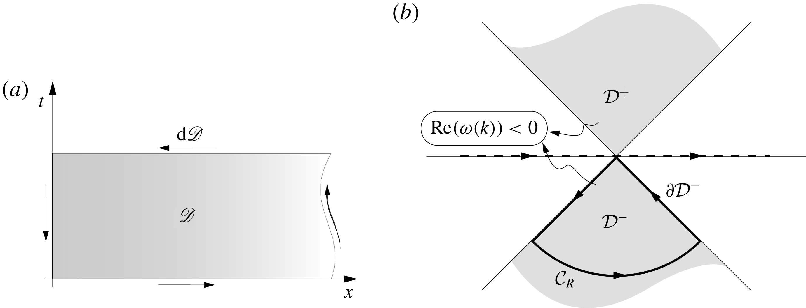
We do this by reformulating the equations of motion of the particle with the non-local history dependence into a local problem for an extended dynamical system. The main principle employed in deriving the extended dynamical system is a domain extension (authors’ work in preparation). In other words, we represent the entirety of the MR equation as a boundary condition to the one-dimensional (1-D) diffusion equation. The extended dynamical system couples three quantities that march in time: the position of the particle, the velocity of the particle, and the field satisfying the diffusion equation (which effectively encodes the history term). The reformulation enables us to write solutions explicitly for spatially uniform fluid flows. We derive explicit expressions for scenarios shown in figure 1(a-d): (i) a particle relaxing in a stationary fluid (in this case, the equations simplify to a constant-coefficient linear problem that can be solved explicitly using a Laplace transform as well; however, even in this case, the solution by that approach is not an explicit function of time, but is given as a convolution integral (Farazmand & Haller Reference Farazmand and Haller2015)); (ii) a particle settling under gravity; (iii) a particle in an oscillating background; and (iv) a particle in planar Couette flow. For short times, we find the particle velocity relaxes faster when the Basset history integral is accounted for than when it is not. Moreover, on accounting for the effect of the history integral, a cross-over time exists beyond which the particle relaxes with a power-law decay, whereas the decay would be exponential without. In the flows we study, we find that, though the transient behaviour of particles in flows is different, the infinite-time behaviour remains unchanged, consistent with the analysis of Langlois et al. (Reference Langlois, Farazmand and Haller2015).
The solution formula that we obtain is of a form where Watson’s lemma (Miller Reference Miller2006) may be applied and hence the large-time behaviour is readily computable. Our reformulation of the MR equation has the additional benefit of being local. This allows us to construct a novel numerical scheme that obviates the issue of rising memory storage. Since the effect of the Basset history integral is accounted for in terms of a dynamical variable, our method may also be employed in large simulations with restarts. In large numerical computations of turbulence, for example in cloud flows, the number of particles considered could be of the order of billions. Our method offers a way of including the Basset history integral into such simulations without an unmanageable increase in storage requirements.
Close to a point vortex (see figure 1
e), upon neglecting the Basset history, the dynamics of particles has been shown to obey a boundary-layer structure (Ravichandran & Govindarajan Reference Ravichandran and Govindarajan2015; Deepu, Ravichandran & Govindarajan Reference Deepu, Ravichandran and Govindarajan2017), where particles initially located within a critical radius
 $r_{c}$
are able to form caustics and evacuate the vicinity of the vortex rapidly, whereas particles initially outside this radius do not form caustics, and so their dynamics may be represented by a velocity field. We define caustics as space–time points where two particles can exist simultaneously with different velocities. We demonstrate our numerical method by studying how the Basset history integral affects caustic formation. We show that the history integral shrinks the critical caustic radius
 $r_{c}$
for all Stokes numbers, but the scaling
 $r_{c}\sim \sqrt{S}$
is unchanged. Lastly, though all the boundary–bulk extension ideas are applied here to MR equations that describe the dynamics of a spherical particle, we show that an exact map can be applied to particles with other geometries such as spheroids and disks in a flow where an analogous Basset history integral exists. We discuss the implications of our findings for turbulent scenarios, where the effect of the Basset history integral on particle clustering is still not clearly understood.
While our present study is devoted to the MR equation, we note that convective inertia effects become important beyond the diffusive time scale (Mei & Adrian Reference Mei and Adrian1992; Lovalenti & Brady Reference Lovalenti and Brady1993a
,Reference Lovalenti and Brady
b
), however small the Reynolds number. So the asymptotic behaviour we calculate below using the MR equation will only be valid up to this time scale, beyond which we must use the entire Navier–Stokes equation to get the correct behaviour. For example, in a particle relaxing to rest in quiescent flow, as calculated in the pioneering work of Lovalenti & Brady (Reference Lovalenti and Brady1993b
), the relaxation behaviour changes from a
 $1/\sqrt{t}$
decay, as predicted by the MR equation with Basset history, to a faster decay of
 $1/t^{2}$
at long times. In the present work, we assume a time scale separation between the history effects arising out of unsteady inertial effects and the time scale due to convective inertial corrections. As a consequence, our long-time asymptotic results are valid at time scales shorter than the convective scale
 $\unicode[STIX]{x1D708}/u_{c}^{2}$
, where
 $u_{c}$
is a characteristic convective velocity. Two situations where there is at least two orders of magnitude of separation between the Stokes and convective time scales and Basset history could be vital to understanding the relevant dynamics; these are droplet growth in cloud flows, and sedimentation of marine snow. It is significant to note that the technique developed here can be extended to account for the convective inertia as well, using a history kernel introduced by Lovalenti & Brady (Reference Lovalenti and Brady1993b
), which will be addressed in future work.
Before we dive into the details of the calculation, we describe our procedure to handle the Basset history term. It is known that the history integral is nothing but a half-derivative in time of the particle velocity relative to fluid motion and it is no surprise that the origin of this half-derivative has to do with the unsteady Stokes equation with particle momentum being diffused by viscosity. On the other hand, it is also known that the half-derivative is the Dirichlet-to-Neumann map for the diffusion equation on the half-line. Let us unpack the previous statement. Suppose
 $\boldsymbol{g}_{0}(t)$
is the Dirichlet condition for a function
 $\boldsymbol{q}(x,t)$
that satisfies the diffusion equation for
 $x>0$
(with zero initial conditions). Then the half-derivative of
 $\boldsymbol{g}_{0}(t)$
is equal to the Neumann condition
 $\boldsymbol{q}_{x}(0,t)$
. This fact allows us to relate the MR equation, which is an ordinary integro-differential equation, to a boundary condition to a diffusion equation. The boundary condition, which is the MR equation itself, is a time-evolving Robin-type boundary condition, and using the unified transform method, as described below, we are immediately able to solve for the particle evolution for arbitrary time-dependent flows.
2 Diffusion equation on half-line
Before we discuss the MR equation itself, we first describe a few results pertaining to the 1-D diffusion equation that are essential to our reformulation of the problem. The unified transform method, alternatively known as the Fokas transform method, is employed in deriving the results in this section. These results are not new. Our intent is to introduce notation as well as the techniques that will be relevant in the following sections. Further details regarding the unified transform method can be found in Fokas (Reference Fokas2008). For a brief introduction to the method, see Deconinck, Trogdon & Vasan (Reference Deconinck, Trogdon and Vasan2014).
Consider the 1-D diffusion equation on a half-line of ‘pseudo’-space
 $x$
with a Dirichlet boundary condition given by
 $\boldsymbol{g}_{0}(t)$
at
 $x=0$
and let
 $\boldsymbol{q}(x,t)$
be the variable that gets diffused. Note that
 $x$
is a fictitious space, not to be confused with the physical space represented by
 $y$
, so we call
 $x$
a pseudo-space. It is used only to establish the relationship between the Basset history integral and the Neumann boundary condition for the diffusion equation. This problem can be formulated in a time interval
 $(0,T]$
as
 $$\begin{eqnarray}\displaystyle \left.\begin{array}{@{}c@{}}\boldsymbol{q}_{t}=\boldsymbol{q}_{xx},\quad x>0,~t\in (0,T],\\ \boldsymbol{q}(x,0)=0,\quad x>0,\\ \boldsymbol{q}(0,t)=\boldsymbol{g}_{0}(t),\quad t\in [0,T].\end{array}\right\} & & \displaystyle\end{eqnarray}$$
Subscripts here denote partial derivatives and the evolution of the variable
 $\boldsymbol{q}(x,t)$
takes place in the
 $x$
–
 $t$
plane in the domain
 $\mathscr{D}$
shown schematically in figure 2(a). As is typical for problems posed on a semi-infinite domain, we assume the field
 $\boldsymbol{q}(x,t)$
vanishes as
 $x\rightarrow \infty$
uniformly for all
 $t$
. Though this problem may be solved using classical techniques, we employ the unified transform method for reasons that will become evident in subsequent sections.
(a) Region
 $\mathscr{D}$
defined by
 $x\in [0,\infty ),~t\in [0,T]$
in which the diffusion equation evolves and
 $\text{d}\mathscr{D}$
is its boundary. (b) Domain
 ${\mathcal{D}}^{\pm }$
where the integrating factor
 $\text{e}^{\unicode[STIX]{x1D714}(k)t}$
decays. The boundary of this region in
 $\mathbb{C}^{-}$
is defined by contour
 $\unicode[STIX]{x2202}{\mathcal{D}}^{-}$
and
 ${\mathcal{C}}_{R}$
whose various contributions help establish the relation between the Dirichlet and Neumann boundary conditions for the diffusion equation.

We begin by rewriting the diffusion equation in its divergence form using the ‘local relation’ (Fokas Reference Fokas2008; Deconinck et al. Reference Deconinck, Trogdon and Vasan2014, Reference Deconinck, Guo, Shlizerman and Vasan2017)
 $$\begin{eqnarray}\displaystyle (\text{e}^{-\text{i}kx+\unicode[STIX]{x1D714}(k)t}\boldsymbol{q})_{t}-(\text{e}^{-\text{i}kx+\unicode[STIX]{x1D714}(k)t}(\boldsymbol{q}_{x}+\text{i}k\boldsymbol{q}))_{x}=0,\quad k\in \mathbb{C}, & & \displaystyle\end{eqnarray}$$
which is valid in any small portion of
 $\mathscr{D}$
where
 $\unicode[STIX]{x1D714}(k)=k^{2}$
. The local relation is simply the diffusion equation multiplied by
 $\text{e}^{-\text{i}kx+\unicode[STIX]{x1D714}(k)t}$
, as one can see by applying the product rule of differentiation to (2.2).
2.1 The global relation and some notation
Next we integrate equation (2.2) over the entirety of
 $\mathscr{D}$
and employ the divergence theorem to obtain a ‘global relation’,
 $$\begin{eqnarray}\displaystyle & & \displaystyle \iint _{\mathscr{D}}[(\text{e}^{-\text{i}kx+\unicode[STIX]{x1D714}(k)t}\boldsymbol{q})_{t}-(\text{e}^{-\text{i}kx+\unicode[STIX]{x1D714}(k)t}(\boldsymbol{q}_{x}+\text{i}k\boldsymbol{q}))_{x}]\,\text{d}x\,\text{d}t=0,\end{eqnarray}$$
 $$\begin{eqnarray}\displaystyle \Rightarrow & & \displaystyle \int _{\text{d}\mathscr{D}}[\text{e}^{-\text{i}kx+\unicode[STIX]{x1D714}(k)t}\boldsymbol{q}\,\text{d}x+\text{e}^{-\text{i}kx+\unicode[STIX]{x1D714}(k)t}(\boldsymbol{q}_{x}+\text{i}k\boldsymbol{q})\,\text{d}t]=0,\end{eqnarray}$$
 $$\begin{eqnarray}\displaystyle \Rightarrow & & \displaystyle \int _{0}^{\infty }\text{e}^{-\text{i}kx}\boldsymbol{q}_{0}(x)\,\text{d}x-\int _{0}^{\infty }\text{e}^{-\text{i}kx+\unicode[STIX]{x1D714}(k)T}\boldsymbol{q}(x,T)\,\text{d}x-\int _{0}^{T}\text{e}^{\unicode[STIX]{x1D714}(k)t}(\boldsymbol{q}_{x}(0,t)+\text{i}k\boldsymbol{g}_{0}(t))\,\text{d}t=0.\nonumber\\ \displaystyle & & \displaystyle\end{eqnarray}$$
The terms at the boundary of
 $\mathscr{D}$
at infinity vanish since
 $\boldsymbol{q}(x,t)\rightarrow 0$
as
 $x\rightarrow \infty$
. Let us define the Fourier transform in pseudo-space as
 $$\begin{eqnarray}\displaystyle \hat{\boldsymbol{q}}_{0}(k) & = & \displaystyle \int _{0}^{\infty }\text{e}^{-\text{i}kx}\boldsymbol{q}_{0}(x)\,\text{d}x,\end{eqnarray}$$
 $$\begin{eqnarray}\displaystyle \hat{\boldsymbol{q}}(k,T) & = & \displaystyle \int _{0}^{\infty }\text{e}^{-\text{i}kx}\boldsymbol{q}(x,T)\,\text{d}x,\end{eqnarray}$$
and the time transform of the boundary terms as
 $$\begin{eqnarray}\displaystyle \tilde{\boldsymbol{g}}_{0}(\unicode[STIX]{x1D714},T) & = & \displaystyle \int _{0}^{T}\text{e}^{\unicode[STIX]{x1D714}(k)t}\boldsymbol{g}_{0}(t)\,\text{d}t,\end{eqnarray}$$
 $$\begin{eqnarray}\displaystyle \tilde{\boldsymbol{g}}_{1}(\unicode[STIX]{x1D714},T) & = & \displaystyle \int _{0}^{T}\text{e}^{\unicode[STIX]{x1D714}(k)t}\boldsymbol{q}_{x}(0,t)\,\text{d}t.\end{eqnarray}$$
Further we define
 ${\mathcal{D}}^{+}$
as
 $$\begin{eqnarray}\displaystyle {\mathcal{D}}^{+}=\{k\in \mathbb{C}:\text{Re}(\unicode[STIX]{x1D714}(k))<0,~\text{Im}(k)>0\}, & & \displaystyle\end{eqnarray}$$
and
 ${\mathcal{D}}^{-}$
as
 $$\begin{eqnarray}\displaystyle {\mathcal{D}}^{+}=\{k\in \mathbb{C}:\text{Re}(\unicode[STIX]{x1D714}(k))<0,~\text{Im}(k)<0\}, & & \displaystyle\end{eqnarray}$$
as shown in figure 2
 $(b)$
. Note that
 $\text{e}^{\unicode[STIX]{x1D714}(k)t}$
is analytic, bounded and decaying for large
 $k$
in these domains, a property we shall use repeatedly. Finally we arrive at the global relation given by
 $$\begin{eqnarray}\displaystyle \hat{\boldsymbol{q}}_{0}(k)-\text{e}^{\unicode[STIX]{x1D714}(k)T}\hat{\boldsymbol{q}}(k,T)-\tilde{\boldsymbol{g}}_{1}-\text{i}k\tilde{\boldsymbol{g}}_{0}=0,\quad k\in \mathbb{C}^{-}. & & \displaystyle\end{eqnarray}$$
Since the initial condition is zero everywhere on the real line, we have
 $$\begin{eqnarray}\displaystyle \text{e}^{\unicode[STIX]{x1D714}(k)T}\hat{\boldsymbol{q}}(k,T)+\tilde{\boldsymbol{g}}_{1}+\text{i}k\tilde{\boldsymbol{g}}_{0}=0,\quad k\in \mathbb{C}^{-}. & & \displaystyle\end{eqnarray}$$
2.2 Dirichlet-to-Neumann map
Equation (2.1) describes the Dirichlet boundary-value problem for the diffusion equation. We now compute the associated Neumann condition, i.e. we ask what Neumann boundary condition would give the same solution as this Dirichlet condition in the entire domain. To do so, we multiply equation (2.13) by
 $\text{i}k\text{e}^{-\unicode[STIX]{x1D714}(k)t}$
for
 $0<t<T$
and integrate over the contour
 $\unicode[STIX]{x2202}{\mathcal{D}}^{-}$
, the boundary of
 ${\mathcal{D}}^{-}$
shown in figure 2(b):
 $$\begin{eqnarray}\displaystyle \int _{\unicode[STIX]{x2202}{\mathcal{D}}^{-}}\left[\text{i}k\int _{0}^{T}\text{e}^{\unicode[STIX]{x1D714}(s-t)}\boldsymbol{q}_{x}(0,s)\,\text{d}s-k^{2}\int _{0}^{T}\text{e}^{\unicode[STIX]{x1D714}(s-t)}\boldsymbol{q}(0,s)\,\text{d}s+\text{i}k\text{e}^{\unicode[STIX]{x1D714}(k)(T-t)}\boldsymbol{q}(k,T)\right]\text{d}k=0. & & \displaystyle \nonumber\\ \displaystyle & & \displaystyle\end{eqnarray}$$
After the manipulations detailed in appendix A, we obtain
 $$\begin{eqnarray}\displaystyle -\unicode[STIX]{x03C0}\boldsymbol{q}_{x}(0,t)-\sqrt{\frac{\unicode[STIX]{x03C0}}{t}}\,\boldsymbol{q}(0,0)-\int _{-\infty }^{\infty }\int _{0}^{t}\text{e}^{-k^{2}(t-s)}\dot{\boldsymbol{q}}(0,s)\,\text{d}s\,\text{d}k=0. & & \displaystyle\end{eqnarray}$$
Setting
 $k^{2}(t-s)=m^{2}$
, where
 $m$
is real, and evaluating the resulting Gaussian integral, we obtain the Dirichlet–Neumann map as
 $$\begin{eqnarray}\displaystyle \boldsymbol{q}_{x}(0,t)=-\sqrt{\frac{1}{\unicode[STIX]{x03C0}t}}\,\boldsymbol{q}(0,0)-\frac{1}{\sqrt{\unicode[STIX]{x03C0}}}\int _{0}^{t}\frac{\dot{\boldsymbol{q}}(0,s)}{\sqrt{t-s}}\,\text{d}s. & & \displaystyle\end{eqnarray}$$
The integral term above is the definition of the Riemann–Liouville half-derivative. This expression relating the Neumann condition for the diffusion equation and the Riemann–Liouville half-derivative forms the basis of our reformulation of the MR equations. More general connections of boundary-value problems to partial differential equations and fractional derivatives are being explored in the authors’ work currently underway.
3 Recasting the Maxey–Riley equation
We may now use (2.16) to rewrite the MR equation (1.2) in its entirety in a reference frame moving with the particle as
 $$\begin{eqnarray}\displaystyle & \displaystyle \dot{\boldsymbol{y}}=\boldsymbol{q}(0,t)+\boldsymbol{u}, & \displaystyle\end{eqnarray}$$
 $$\begin{eqnarray}\displaystyle & \displaystyle \boldsymbol{q}_{t}(0,t)+\unicode[STIX]{x1D6FC}\boldsymbol{q}(0,t)-\unicode[STIX]{x1D6FE}\boldsymbol{q}_{x}(0,t)=\boldsymbol{f}(\boldsymbol{q}(0,t),\boldsymbol{y},t), & \displaystyle\end{eqnarray}$$
 $$\begin{eqnarray}\displaystyle \unicode[STIX]{x1D6FC}=\frac{1}{RS},\quad \unicode[STIX]{x1D6FE}=\frac{1}{R}\sqrt{\frac{3}{S}},\quad \boldsymbol{f}(\boldsymbol{q}(0,t),\boldsymbol{y}(t),t)=\left(\frac{1}{R}-1\right)\frac{\text{D}\boldsymbol{u}}{\text{D}t}-\boldsymbol{q}(0,t)\boldsymbol{\cdot }\unicode[STIX]{x1D735}\boldsymbol{u}, & & \displaystyle\end{eqnarray}$$
where
 $\boldsymbol{q}(0,t)=\boldsymbol{v}(t)-\boldsymbol{u}(\boldsymbol{y}(t),t)$
is the relative velocity of the particle. In this choice of reference frame, with the history term on the left-hand side in (3.2), we are left with a forcing function
 $\boldsymbol{f}$
that is local in time, whereas in the original form (1.2) forcing appeared in a non-local manner. As
 $\boldsymbol{q}(0,t)$
and
 $\boldsymbol{q}_{x}(0,t)$
represent the Dirichlet and Neumann conditions of a field satisfying the diffusion equation, we are naturally led to consider the following boundary-value problem:
 $$\begin{eqnarray}\displaystyle & \displaystyle \boldsymbol{q}_{t}=\boldsymbol{q}_{xx},\quad x>0,~t\in (0,T], & \displaystyle\end{eqnarray}$$
 $$\begin{eqnarray}\displaystyle & \displaystyle \boldsymbol{q}(x,0)=0,\quad x>0, & \displaystyle\end{eqnarray}$$
 $$\begin{eqnarray}\displaystyle & \displaystyle \boldsymbol{q}_{t}(0,t)+\unicode[STIX]{x1D6FC}\boldsymbol{q}(0,t)-\unicode[STIX]{x1D6FE}\boldsymbol{q}_{x}(0,t)=\boldsymbol{f}(\boldsymbol{q}(0,t),\boldsymbol{y},t),\quad t\in [0,T], & \displaystyle\end{eqnarray}$$
 $$\begin{eqnarray}\displaystyle & \displaystyle \dot{\boldsymbol{y}}(t)=\boldsymbol{q}(0,t)+\boldsymbol{u}(\boldsymbol{y}(t)),\quad t\in [0,T], & \displaystyle\end{eqnarray}$$
 $$\begin{eqnarray}\displaystyle & \displaystyle \lim _{t\rightarrow 0}\boldsymbol{q}(0,t)=\boldsymbol{v}_{0}, & \displaystyle\end{eqnarray}$$
 $$\begin{eqnarray}\displaystyle & \displaystyle \boldsymbol{y}(0)=\boldsymbol{y}_{0}. & \displaystyle\end{eqnarray}$$
The MR equation (1.2) thus manifests itself as a nonlinear modified Robin boundary condition, on the time axis of figure 2(a), to the diffusion equation. We do not yet know
 $\boldsymbol{q}(0,t)$
on this axis, i.e. the particle velocity in the relative frame of reference, for which we derive an expression in the next subsection. From here on we work with this form of the MR equation and the global relation (2.13) for the diffusion equation. Higher-order corrections in particle size, the Faxén correction, etc. can also be accommodated in the forcing expression,
 $\boldsymbol{f}(\boldsymbol{q}(0,t),\boldsymbol{y},t)$
. Here
 $\boldsymbol{u}$
is a known velocity field. In the general case, one would couple the MR equation with a fluid model (such as the Navier–Stokes equation) to simultaneously resolve particle locations and fluid velocities. An example of this kind, in the form of particles around a point vortex, is studied in a later section.
3.1 Solution for time-dependent forcing
The form of the MR equation (3.2)–(3.3) suggests that the forcing function is both space- and time-dependent. However, it is instructive and useful to first study a case when the forcing is a function of time alone, i.e.
 $\boldsymbol{f}(t)$
. The ideas presented here will be extended to more complicated scenarios in later sections.
Using the definitions (2.8)–(2.9), we take the time transform of the boundary condition (3.6) and after integrating by parts we get
 $$\begin{eqnarray}\displaystyle (\text{e}^{\unicode[STIX]{x1D714}(k)T}\boldsymbol{q}(0,T)-\boldsymbol{v}_{0})+(\unicode[STIX]{x1D6FC}-k^{2})\tilde{\boldsymbol{g}}_{0}-\unicode[STIX]{x1D6FE}\tilde{\boldsymbol{g}}_{1}=\,\tilde{\boldsymbol{f}}. & & \displaystyle\end{eqnarray}$$
Here
 $\tilde{\boldsymbol{f}}$
is the time transform of the function
 $\boldsymbol{f}$
. Using the global relation (2.13), we eliminate
 $\tilde{\boldsymbol{g}}_{1}$
from the above expression and multiply the resulting equality by
 $\text{i}k\text{e}^{-\unicode[STIX]{x1D714}(k)t}$
for
 $0<t<T$
and finally integrate over
 $\unicode[STIX]{x2202}{\mathcal{D}}^{-}$
. This leads to
 $$\begin{eqnarray}\displaystyle \int _{\unicode[STIX]{x2202}{\mathcal{D}}^{-}}\text{i}k\tilde{\boldsymbol{g}}_{0}(\unicode[STIX]{x1D714},T)\text{e}^{-\unicode[STIX]{x1D714}(k)t}\,\text{d}k=\int _{\unicode[STIX]{x2202}{\mathcal{D}}^{-}}\text{i}k\text{e}^{-\unicode[STIX]{x1D714}(k)t}\left[\frac{\,\tilde{\boldsymbol{f}}-\text{e}^{\unicode[STIX]{x1D714}T}\boldsymbol{q}(0,T)+\boldsymbol{v}_{0}-\unicode[STIX]{x1D6FE}\text{e}^{\unicode[STIX]{x1D714}T}\hat{\boldsymbol{q}}(k,T)}{\unicode[STIX]{x1D6FC}-k^{2}+\text{i}k\unicode[STIX]{x1D6FE}}\right]\text{d}k, & & \displaystyle \nonumber\\ \displaystyle & & \displaystyle\end{eqnarray}$$
 $$\begin{eqnarray}\displaystyle & & \displaystyle \int _{\unicode[STIX]{x2202}{\mathcal{D}}^{-}}\text{i}k\text{e}^{-k^{2}t}\int _{0}^{T}\text{e}^{k^{2}s}\boldsymbol{q}(0,s)\,\text{d}s\,\text{d}k\nonumber\\ \displaystyle & & \displaystyle \quad =\int _{\unicode[STIX]{x2202}{\mathcal{D}}^{-}}\frac{\text{i}k\text{e}^{-k^{2}t}(\,\tilde{\boldsymbol{f}}(k,T)+\boldsymbol{v}_{0})}{\unicode[STIX]{x1D6FC}-k^{2}+\text{i}k\unicode[STIX]{x1D6FE}}\,\text{d}k-\int _{\unicode[STIX]{x2202}{\mathcal{D}}^{-}}\text{i}k\frac{\text{e}^{k^{2}(T-t)}(\boldsymbol{q}(0,T)+\unicode[STIX]{x1D6FE}\hat{\boldsymbol{q}}(k,T))}{\unicode[STIX]{x1D6FC}-k^{2}+\text{i}k\unicode[STIX]{x1D6FE}}\,\text{d}k,\end{eqnarray}$$
where (in the second line) we have used the definition of
 $\tilde{\boldsymbol{g}}_{0}$
and the fact that
 $\unicode[STIX]{x1D714}(k)=k^{2}$
. We substitute
 $k^{2}=\text{i}l$
in the left-hand-side term above, which describes the boundary
 $\unicode[STIX]{x2202}{\mathcal{D}}^{-}$
, see figure 2(b), to arrive at
 $$\begin{eqnarray}\displaystyle & & \displaystyle -\frac{1}{2}\int _{-\infty }^{\infty }\text{e}^{-\text{i}l(t-s)}\int _{0}^{T}\boldsymbol{q}(0,s)\,\text{d}l\,\text{d}s\nonumber\\ \displaystyle & & \displaystyle \quad =\int _{\unicode[STIX]{x2202}{\mathcal{D}}^{-}}\frac{\text{i}k\text{e}^{-k^{2}t}(\,\tilde{\boldsymbol{f}}(k,T)+\boldsymbol{v}_{0})}{\unicode[STIX]{x1D6FC}-k^{2}+\text{i}k\unicode[STIX]{x1D6FE}}\,\text{d}k-\int _{\unicode[STIX]{x2202}{\mathcal{D}}^{-}}\text{i}k\frac{\text{e}^{k^{2}(T-t)}(\boldsymbol{q}(0,T)+\unicode[STIX]{x1D6FE}\hat{\boldsymbol{q}}(k,T))}{\unicode[STIX]{x1D6FC}-k^{2}+\text{i}k\unicode[STIX]{x1D6FE}}\,\text{d}k,\end{eqnarray}$$
 $$\begin{eqnarray}\displaystyle -\unicode[STIX]{x03C0}\boldsymbol{q}(0,t) & = & \displaystyle \int _{\unicode[STIX]{x2202}{\mathcal{D}}^{-}}\int _{0}^{t}\frac{\text{i}k\text{e}^{-k^{2}(t-s)}\boldsymbol{f}(s)}{\unicode[STIX]{x1D6FC}-k^{2}+\text{i}k\unicode[STIX]{x1D6FE}}\,\text{d}k\,\text{d}s+\int _{\unicode[STIX]{x2202}{\mathcal{D}}^{-}}\frac{\boldsymbol{v}_{0}\text{i}k\text{e}^{-k^{2}t}}{\unicode[STIX]{x1D6FC}-k^{2}+\text{i}k\unicode[STIX]{x1D6FE}}\,\text{d}k\nonumber\\ \displaystyle & & \displaystyle +\int _{\unicode[STIX]{x2202}{\mathcal{D}}^{-}}\int _{t}^{T}\frac{\text{i}k\text{e}^{k^{2}(s-t)}\boldsymbol{f}(s)}{\unicode[STIX]{x1D6FC}-k^{2}+\text{i}k\unicode[STIX]{x1D6FE}}\,\text{d}k\,\text{d}s\nonumber\\ \displaystyle & & \displaystyle -\int _{\unicode[STIX]{x2202}{\mathcal{D}}^{-}}\text{i}k\frac{\text{e}^{k^{2}(T-t)}(\boldsymbol{q}(0,T)+\unicode[STIX]{x1D6FE}\hat{\boldsymbol{q}}(k,T))}{\unicode[STIX]{x1D6FC}-k^{2}+\text{i}k\unicode[STIX]{x1D6FE}}\,\text{d}k,\end{eqnarray}$$
where we have used the standard Fourier inversion formula on the left-hand side. There are two poles due to the quadratic in the denominator of the above equation which are located at
 $$\begin{eqnarray}\displaystyle k_{\pm }={\textstyle \frac{1}{2}}(\text{i}\unicode[STIX]{x1D6FE}\pm \sqrt{4\unicode[STIX]{x1D6FC}-\unicode[STIX]{x1D6FE}^{2}}\,). & & \displaystyle\end{eqnarray}$$
Since both
 $\unicode[STIX]{x1D6FE}$
and
 $\unicode[STIX]{x1D6FC}$
are positive parameters, the poles
 $k_{\pm }$
always lie in
 $\mathbb{C}^{+}$
and reach the real line for
 $\unicode[STIX]{x1D6FE}=0$
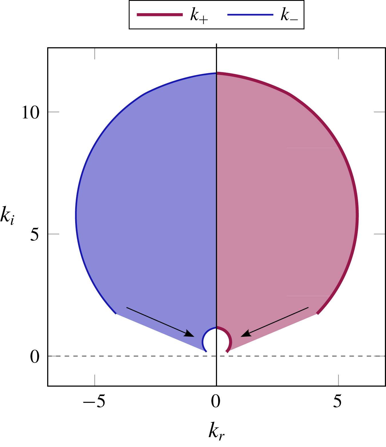
, i.e. when Basset history is absent (see figure 3). An appeal to Jordan’s lemma (Ablowitz & Fokas Reference Ablowitz and Fokas2003, p. 222) shows that the third and fourth terms (those involving function evaluations at
 $T$
) in equation (3.14) do not contribute, since
 $k^{2}$
is negative in
 ${\mathcal{D}}^{-}$
and
 $(t-s)>0$
. It is not surprising that these two terms do not contribute, as this only ensures causality: the dynamics of the particle for all times
 $t<T$
cannot depend on a quantity from future time
 $T$
. Using the fact that
 $\text{e}^{-k^{2}t}$
is decaying in the region outside
 ${\mathcal{D}}^{-}$
, we can write the final solution expression as
 $$\begin{eqnarray}\displaystyle -\unicode[STIX]{x03C0}\boldsymbol{q}(0,t)=\int _{\unicode[STIX]{x2202}{\mathcal{D}}^{-}}\int _{0}^{t}\frac{\text{i}k\text{e}^{-k^{2}(t-s)}\boldsymbol{f}(s)}{\unicode[STIX]{x1D6FC}-k^{2}+\text{i}k\unicode[STIX]{x1D6FE}}\,\text{d}s\,\text{d}k-\int _{-\infty }^{\infty }\frac{\boldsymbol{v}_{0}\text{i}k\text{e}^{-k^{2}t}}{\unicode[STIX]{x1D6FC}-k^{2}+\text{i}k\unicode[STIX]{x1D6FE}}\,\text{d}k. & & \displaystyle\end{eqnarray}$$
Note that the particle velocity is now given by the above expression directly (and explicitly) in terms of the initial condition
 $\boldsymbol{v}_{0}~(=\boldsymbol{v}(0)-\boldsymbol{u}(0))$
and the forcing
 $\boldsymbol{f}(t)$
in the relative frame of reference. The quantity
 $\boldsymbol{q}(0,t)$
represents the Dirichlet boundary condition for the modified Robin boundary-value problem for the diffusion equation. Once the relative velocity
 $\boldsymbol{q}(0,t)$
is available, one may readily compute particle trajectories
 $\boldsymbol{y}(t)$
from (3.7).
The region in
 $k\in \mathbb{C}^{+}$
where the poles
 $k_{\pm }$
from (3.15) are located for Stokes number
 $S$
in the range 0.01–1 and density ratios corresponding to
 $R$
in the range
 $1/3$
–5. As the Stokes number increases, the poles approach the real line shown using arrows, and similarly as we increase the density ratio. Note that, without Basset history, the poles would merely lie symmetrically on the
 $k_{r}$
line.

Without the unified transform method, one may not have suspected such a boundary-value problem is indeed solvable. Of course, one could in principle have employed the Laplace transform to obtain the solution, though a couple of issues arise then. If one were to use the Laplace transform, the inverse would involve branch cuts in the general case, which are difficult to evaluate, and, as mentioned above, explicit solutions are most often not possible. However, the unified transform method provides the appropriate reparametrisation to avoid these complications, and to further provide an explicit expression in
 $t$
for the solution, given by (3.16). As we shall see in the following sections, especially when considering the nonlinear problem
 $\boldsymbol{f}(\boldsymbol{q}(0,t),\boldsymbol{y},t)$
, the true benefit of adopting the new formulation is the local nature of the extended system, which is precisely due to the connection between the MR equations and the diffusion equation.
4 Explicit solution for particular flows
In several fluid scenarios, there is a considerable separation between diffusive and convective time scales. Two such examples are highlighted below. In such scenarios, the Basset history force has a non-negligible effect on the resultant particle dynamics. Consequently, we present several example flows which permit explicit treatment of the Basset history term and its impact on the particle motion.
(a) Clouds. In clouds, the particle time scale
 $\unicode[STIX]{x1D70F}_{p}$
for a droplet of size
$a\sim 10~\unicode[STIX]{x03BC}\text{m}$
is
$O(\unicode[STIX]{x03BC}\text{s})$
, while the energy dissipation occurring at Kolmogorov scale has a time scale
$\unicode[STIX]{x1D70F}_{in}\sim O(\text{ms})$
. Ling, Parmar & Balachandar (Reference Ling, Parmar and Balachandar2013) showed that, when the transition time scale (given by
$\unicode[STIX]{x1D70F}_{t}$
) from slow diffusive relaxation to fast inertial relaxation is larger than
$\unicode[STIX]{x1D70F}_{in}$
, then history effects due to viscous diffusion are important in such turbulent scenarios. It can easily be computed for a typical cloud droplet of
$10~\unicode[STIX]{x03BC}\text{m}$
that
$\unicode[STIX]{x1D70F}_{in}/\unicode[STIX]{x1D70F}_{t}\sim O(0.1)$
, which clearly is in the limit where particle dynamics is dominated by history effects. Moreover, since
$\unicode[STIX]{x1D70F}_{in}$
is the smallest time scale in the flow, time scales of eddies on the size of the Kolmogorov length scale, or larger, are greater than
$\unicode[STIX]{x1D70F}_{in}$
. The analysis of Balachandar (Reference Balachandar2009) and Ling et al. (Reference Ling, Parmar and Balachandar2013) thus suggests that the full history kernel is then well approximated by the Basset-like slower
$t^{-1/2}$
kernel.
(b) Plankton. Plankton in the ocean come in various sizes and different density ratios. The effect of turbulence on clustering (Guseva et al. Reference Guseva, Daitche, Feudel and Tél2016) is poorly understood, and we believe that Basset history, given its non-trivial dynamics, might play a role in its settling. A plankton of size
$a\sim 100~\unicode[STIX]{x03BC}\text{m}$
has a terminal velocity of
$U_{t}\sim 0.1~\text{mm}~\text{s}^{-1}$
when
$\unicode[STIX]{x0394}\unicode[STIX]{x1D70C}/\unicode[STIX]{x1D70C}\sim 0.1$
(where
$\unicode[STIX]{x0394}\unicode[STIX]{x1D70C}$
is the difference between particle density and fluid density, with
$\unicode[STIX]{x1D70C}$
being the density of water). The diffusive time scale
$a^{2}/\unicode[STIX]{x1D708}\sim 1~\text{s}$
while
$\unicode[STIX]{x1D70F}_{in}=\unicode[STIX]{x1D708}/U_{t}^{2}\sim O(\text{h})$
. This clearly shows that such a huge time scale separation makes studying Basset history effects worth while. Also we suspect that the clustering of plankton could happen in a short time, dynamics being dominated by diffusive effects.


Given this motivation, we start looking at simple scenarios where fluid velocity is only time-dependent and space-independent as we build onto complex flows.
4.1 Example 1: relaxing particle
In the absence of a background flow (namely when
 $\boldsymbol{f}=0$
), expression (3.16) for the relative velocity
 $\boldsymbol{q}(0,t)$
may be analysed using Watson’s lemma. Since the real line in
 $k$
happens to be the path of steepest descent, Laplace’s method provides the asymptotic behaviour for functions of the form
 $$\begin{eqnarray}\displaystyle \mathscr{K}(\unicode[STIX]{x1D701}):=\int _{a}^{b}\text{e}^{g(\unicode[STIX]{x1D701})t}\unicode[STIX]{x1D713}(\unicode[STIX]{x1D701})\,\text{d}\unicode[STIX]{x1D701}\quad \text{as}~t\rightarrow \infty ,~t>0, & & \displaystyle\end{eqnarray}$$
in terms of the local maximum value of the function
 $g(\unicode[STIX]{x1D701})$
when
 $\unicode[STIX]{x1D701}\in [a,b]$
. This leads to the well-known asymptotic result for integrals of the above form:
 $$\begin{eqnarray}\displaystyle \mathscr{K}(\unicode[STIX]{x1D701}):=\int _{-\infty }^{\infty }\text{e}^{-\unicode[STIX]{x1D701}^{2}t}\unicode[STIX]{x1D713}(\unicode[STIX]{x1D701})\,\text{d}\unicode[STIX]{x1D701}~\approx ~\sqrt{\frac{\unicode[STIX]{x03C0}}{t}}\mathop{\sum }_{n=0}^{\infty }\frac{\unicode[STIX]{x1D713}_{k}(0)}{2^{2n}n!}\,t^{-n},\quad \text{as}~t\rightarrow \infty . & & \displaystyle\end{eqnarray}$$
On setting
 $\boldsymbol{f}=0$
we see that the dominant contribution of the integral in (3.16) comes from
 $k=0$
. To leading order we have
 $$\begin{eqnarray}\displaystyle \boldsymbol{q}(0,t)\approx \frac{\boldsymbol{v}_{0}}{\sqrt{\unicode[STIX]{x03C0}}t^{3/2}}\,\frac{\unicode[STIX]{x1D6FE}}{2\unicode[STIX]{x1D6FC}^{2}}+O(t^{-5/2}),\quad t\gg 0. & & \displaystyle\end{eqnarray}$$
Farazmand & Haller (Reference Farazmand and Haller2015) and Langlois et al. (Reference Langlois, Farazmand and Haller2015) approached this problem by using a Laplace transform. Their complete solution was provided in terms of convolutions and not directly as we obtain in (3.16). For large times, however, Langlois et al. (Reference Langlois, Farazmand and Haller2015) present the same equation as (4.3). Their solution for a relaxing particle is the only earlier closed-form solution that we know of, which accounts for the initial conditions correctly. We contrast the complete solution (3.16) with the one obtained upon neglecting the Basset history integral in the original MR equation. This is equivalent to neglecting the Neumann term
 $\boldsymbol{q}_{x}(0,t)$
in (3.10) and repeating the calculation of
 $\boldsymbol{q}(0,t)$
. Alternatively, we just set
 $\unicode[STIX]{x1D6FE}=0$
in (3.16) to obtain
 $$\begin{eqnarray}\displaystyle \unicode[STIX]{x03C0}\boldsymbol{q}(0,t)=\int _{-\infty }^{\infty }\frac{\boldsymbol{v}_{0}\text{i}k\text{e}^{-k^{2}t}}{k^{2}-\unicode[STIX]{x1D6FC}}\,\text{d}k. & & \displaystyle\end{eqnarray}$$
The non-zero contribution to the integrand comes only from the poles as the integrand is odd, leading to
 $$\begin{eqnarray}\displaystyle \boldsymbol{q}(0,t)=\boldsymbol{v}_{0}\text{e}^{-\unicode[STIX]{x1D6FC}t}, & & \displaystyle\end{eqnarray}$$
and is precisely the expression one gets by solving the MR equation directly without the history term (and
 $\boldsymbol{f}=0$
).
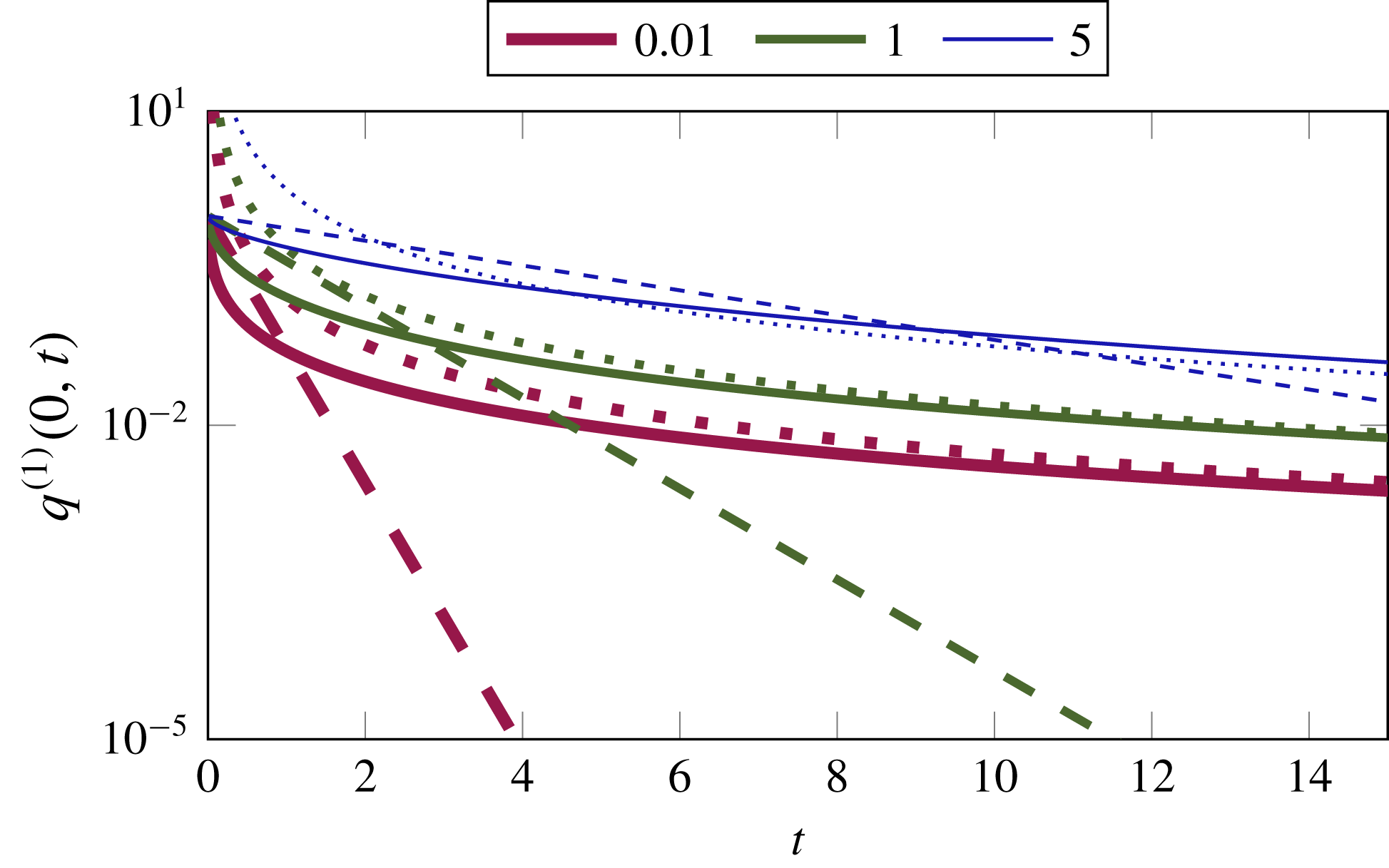
Particle velocity with (solid lines) and without (dashed lines) Basset history, along with the asymptotic solution (dotted lines) from (4.3). The curves from bottom to top, respectively, correspond to three different density ratios, at a fixed Stokes number of
 $S=1$
: light particles, with
 $\unicode[STIX]{x1D6FD}=\unicode[STIX]{x1D71A}_{p}/\unicode[STIX]{x1D71A}_{f}=0.01$
; neutrally buoyant particles, with
 $\unicode[STIX]{x1D6FD}=1$
; and heavy particles, with
 $\unicode[STIX]{x1D6FD}=5$
. The decay rate of particle velocity goes as
 $t^{-3/2}$
for long times when Basset history is accounted for, in contrast to the exponential decay when it is neglected.

In figure 4 we plot the velocity obtained both by including the history integral and by excluding it for three cases: neutrally buoyant (
 $\unicode[STIX]{x1D6FD}=1$
), light (
 $\unicode[STIX]{x1D6FD}=0.01$
) and heavy (
 $\unicode[STIX]{x1D6FD}=5$
) particles. Two important features are evident. First, the solution with Basset history settles not exponentially but as a power law (in this case a very slow
 $t^{-3/2}$
). Secondly, there exists a cross-over time prior to which a particle evolving under the influence of the Basset history integral and Stokes drag relaxes faster than a particle evolving only under Stokes drag. However, after the cross-over time the particle that evolves only under Stokes drag relaxes faster. This contradicts the popular notion that Basset history acts as an effective drag. Thus far, for this example, we have considered the effect of varying density ratios on the particle relaxation time. Note that varying the Stokes number does not lead to substantially different velocity profiles since the Stokes number may be scaled out of the solution by replacing
 $k\rightarrow \tilde{k}/\sqrt{S}$
and
 $t\rightarrow \tilde{t}S$
. Particle velocities for Stokes number
 $S\neq 1$
may be obtained from those depicted in figure 4 by suitably scaling time.
4.2 Example 2: sedimenting particle
The dynamics of particles settling under gravity is relevant in industrial applications, for aerosol particles and droplets in the Earth’s atmosphere, and for carbon sequestration by marine snow in the oceans. In this section a two-dimensional (2-D) flow is considered, with a superscript
 $(\cdot )^{(2)}$
indicating the vertical component of the relevant vector, while
 $(\cdot )^{(1)}$
indicates the horizontal component. When the particle is acted upon by a body force such as gravity, the vertical component of the forcing function
 $\boldsymbol{f}$
,
 $f^{(2)}(t)$
, is a constant of magnitude
 $\unicode[STIX]{x1D70E}$
. This allows us to evaluate the time transform explicitly as
 $$\begin{eqnarray}\displaystyle \tilde{f}^{(2)}(\unicode[STIX]{x1D714},T)=\int _{0}^{T}\unicode[STIX]{x1D70E}\text{e}^{\unicode[STIX]{x1D714}s}\,\text{d}s=\frac{\unicode[STIX]{x1D70E}(\text{e}^{\unicode[STIX]{x1D714}T}-1)}{\unicode[STIX]{x1D714}}. & & \displaystyle\end{eqnarray}$$
The settling velocity of the particle is
 $$\begin{eqnarray}\displaystyle \unicode[STIX]{x03C0}q^{(2)}(0,t)=\int _{-\infty }^{\infty }\frac{\text{i}k\text{e}^{-k^{2}t}v_{0}^{(2)}}{\unicode[STIX]{x1D6FC}-k^{2}+\text{i}k\unicode[STIX]{x1D6FE}}\,\text{d}k+\int _{-\infty }^{\infty }\frac{\unicode[STIX]{x1D70E}\unicode[STIX]{x1D6FE}(1-\text{e}^{-k^{2}t})}{(\unicode[STIX]{x1D6FC}-k^{2})^{2}+k^{2}\unicode[STIX]{x1D6FE}^{2}}\,\text{d}k. & & \displaystyle\end{eqnarray}$$
A solution for this problem is provided in Clift et al. (Reference Clift, Grace and Weber2005). However, their solution necessitates a condition of zero initial velocity for the particle. Moreover, their solution is in terms of sums of error functions, and so the asymptotic form for large time is difficult to glean directly. We evaluate the full solution (4.7), without the requirement for zero initial velocity, for the same particle density ratios as in the previous example (but fixed Stokes number
 $S=0.01$
), corresponding to neutrally buoyant, light and heavy particles:
 $\unicode[STIX]{x1D6FD}=1$
, 0.01 and 5, respectively (see figure 5
a,b). We also obtain the leading-order asymptotic behaviour for the particle velocity as
 $$\begin{eqnarray}\displaystyle q^{(2)}(0,t) & {\approx} & \displaystyle c(\unicode[STIX]{x1D6FC},\unicode[STIX]{x1D6FE})+\frac{\unicode[STIX]{x1D70E}\unicode[STIX]{x1D6FE}}{\unicode[STIX]{x1D6FC}^{2}(\unicode[STIX]{x03C0}t)^{1/2}}+O(t^{-3/2}),\quad t\gg 0,\end{eqnarray}$$
 $$\begin{eqnarray}\displaystyle c(\unicode[STIX]{x1D6FC},\unicode[STIX]{x1D6FE}) & = & \displaystyle \int _{-\infty }^{\infty }\frac{\unicode[STIX]{x1D70E}\unicode[STIX]{x1D6FE}}{(\unicode[STIX]{x1D6FC}-k^{2})^{2}+k^{2}\unicode[STIX]{x1D6FE}^{2}}\,\text{d}k=\frac{\unicode[STIX]{x03C0}\unicode[STIX]{x1D70E}}{\unicode[STIX]{x1D6FC}},\end{eqnarray}$$
where
 $c(\unicode[STIX]{x1D6FC},\unicode[STIX]{x1D6FE})$
is the velocity of the sedimenting particle at long times.
(a) Particle velocity relative to fluid,
 $q^{(2)}(0,t)$
, along the
 $y^{(2)}$
-direction and (b) particle trajectory as a function of time for three density ratios,
 $\unicode[STIX]{x1D6FD}=0.01,1,5$
, corresponding to light, neutrally buoyant and heavy particle when acted upon by gravity for
 $S=0.01,~\unicode[STIX]{x1D70E}=-1$
in (4.7). The asymptotic expression for velocity in (4.9) is plotted as the dotted line in (a), and the dashed line in (b) is the trajectory of the particle without accounting for Basset history. The time taken by particles to reach
 $y^{(2)}=0$
when accounting for Basset history for these density ratios is
 $t=1.1,1.15,1.2$
and without Basset history it takes
 $t=1,1.01,1.04$
.

Note that the terminal velocity
 $c(\unicode[STIX]{x1D6FC},\unicode[STIX]{x1D6FE})$
is in fact the same quantity as that obtained for a particle in the absence of the Basset history force and, more importantly, this terminal velocity is independent of
 $\unicode[STIX]{x1D6FE}$
. The expression
 $\unicode[STIX]{x1D70E}\unicode[STIX]{x03C0}/\unicode[STIX]{x1D6FC}$
is the constant velocity obtained from a balance of gravitational forces and steady drag in our notation. The evaluation of the integral expression for
 $c(\unicode[STIX]{x1D6FC},\unicode[STIX]{x1D6FE})$
is via an appeal to the residue theorem, albeit for three different cases:
 $\unicode[STIX]{x1D6FE}^{2}/\unicode[STIX]{x1D6FC}<4$
,
 $\unicode[STIX]{x1D6FE}^{2}/\unicode[STIX]{x1D6FC}=4$
and
 $\unicode[STIX]{x1D6FE}^{2}/\unicode[STIX]{x1D6FC}>4$
. In all three cases, the integral has the same value.
We observe that a sedimenting particle attains its terminal velocity at a rate of
 $t^{-1/2}$
, which is far slower than the exponential trend as predicted without Basset history. It is worth noting that a sedimenting particle’s relaxation is even slower than the
 $t^{-3/2}$
trend observed for the force-free relaxation (4.3). Another interesting feature of this dynamics, which would be missed on neglecting the Basset history integral, is that the long-time trajectory of the particle is given by
 $y^{(2)}\sim -1/(y^{(1)}-\unicode[STIX]{x1D709})$
(with
 $\unicode[STIX]{x1D709}$
being the final horizontal coordinate). This behaviour is anomalous in the sense that it is neither projectile nor ballistic.
The previous remarks suggest that Basset history could play a significant role in complex flows. For example, the sedimentation rates of individual particles will determine how frequently particles collide with one another and coalesce as they sink. This question is of importance to estimating carbon sequestration by plankton in the ocean, for raindrop growth, and for pulverised coal in thermal power plants. To this end, here we make a simple estimate for how a particle grows in size as it sediments through a sea of smaller particles.
It is simpler in this case to work with the dimensional equation, obtained by replacing
 $\unicode[STIX]{x1D70E}\rightarrow (\unicode[STIX]{x1D6FD}-1)g/R$
and
 $S\rightarrow \unicode[STIX]{x1D70F}_{p}$
, where
 $g$
is gravity and
 $\unicode[STIX]{x1D70F}_{p}=a^{2}/\unicode[STIX]{x1D708}$
is the particle time scale, so (4.7) reads as
 $$\begin{eqnarray}\displaystyle \unicode[STIX]{x03C0}q^{(2)}(0,t)=\int _{-\infty }^{\infty }\frac{\text{i}k\text{e}^{-k^{2}t}v_{0}^{(2)}}{\displaystyle \frac{1}{R\unicode[STIX]{x1D70F}_{p}}-k^{2}+\frac{\text{i}k}{R\sqrt{\unicode[STIX]{x1D70F}_{p}}}}\,\text{d}k-\int _{-\infty }^{\infty }\frac{\displaystyle \frac{(\unicode[STIX]{x1D6FD}-1)g}{R^{2}\sqrt{\unicode[STIX]{x1D70F}_{p}}}(1-\text{e}^{k^{2}t})}{\left(\displaystyle \frac{1}{R\unicode[STIX]{x1D70F}_{p}}-k^{2}\right)^{2}+\displaystyle \frac{k^{2}}{R^{2}\unicode[STIX]{x1D70F}_{p}}}\,\text{d}k. & & \displaystyle\end{eqnarray}$$
Now
 $k$
has the dimensions of
 $t^{-1/2}$
, and
 $v_{0}^{(2)}$
and
 $q^{(2)}(0,t)$
are dimensional velocities. We follow one large particle of growing radius
 $a$
as it sediments through a quiescent fluid with a uniform distribution of identical small particles of radius
 $a_{s}<a$
occupying a solid fraction
 $\unicode[STIX]{x1D711}$
. The larger particle falls faster than the smaller ones, and in a short time
 $\unicode[STIX]{x0394}t$
it collides with all small particles whose centres lie within a cylinder of radius
 $(a+a_{s})$
and height
 $q^{(2)}(0,t)\unicode[STIX]{x0394}t$
. Assuming that all small particles it collides with will coalesce with the bigger particle and that
 $a\gg a_{s}$
, its volume increases by
 $\unicode[STIX]{x1D711}\unicode[STIX]{x03C0}a^{2}q^{(2)}(0,t)\unicode[STIX]{x0394}t$
. Thus we get an evolution for the particle time scale as
 $$\begin{eqnarray}\displaystyle \unicode[STIX]{x1D70F}_{p}^{(n)}=\left(\unicode[STIX]{x1D70F}_{p}^{3/2}+\frac{3}{4}\unicode[STIX]{x1D711}\unicode[STIX]{x1D70F}_{p}\frac{q^{(2)}(0,t)\unicode[STIX]{x0394}t}{\sqrt{\unicode[STIX]{x1D708}}}\right)^{2/3}, & & \displaystyle\end{eqnarray}$$
which modifies
 $\unicode[STIX]{x1D6FC}$
and
 $\unicode[STIX]{x1D6FE}$
in (3.16). After each time interval
 $\unicode[STIX]{x0394}t$
, we reinitialise the system with a new initial condition
 $v_{0}^{(2)}$
, being the velocity from the previous time instant, and a new relaxation time
 $\unicode[STIX]{x1D70F}_{p}^{(n)}$
. For a droplet of
 $\unicode[STIX]{x1D708}\sim 10^{-5}~\text{m}^{2}~\text{s}^{-1}$
,
 $a\sim 0.3$
mm and
 $\unicode[STIX]{x1D6FD}=10$
, we get
 $\unicode[STIX]{x1D70F}_{p}\sim 10^{-2}$
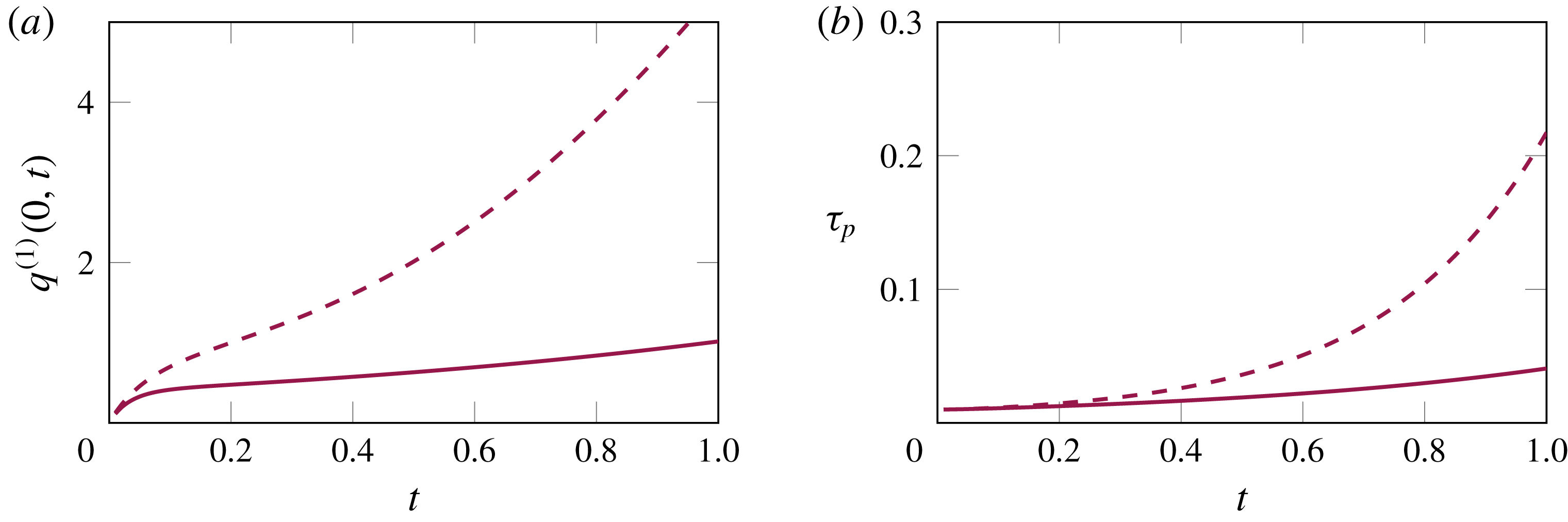
s. In figure 6(a) we plot the dynamics of such a particle; and in figure 6(b) the particle size is represented in terms of its time scale
 $\unicode[STIX]{x1D70F}_{p}$
as a function of time for two scenarios: accounting for (i) history effects (solid lines) and (ii) only Stokes drag (dashed lines). We see that by neglecting the history force we will grossly overestimate particle size at a given time.
(a) Velocity as a function of time of a particle growing in size as it sediments through a uniform distribution of smaller particles and coalesces with those it collides with. (b) The size of this particle as a function of time in terms of its relaxation time scale
 $\unicode[STIX]{x1D70F}_{p}$
with initial
 $\unicode[STIX]{x1D70F}_{p}=0.01$
s,
 $v_{0}^{(2)}=0.01$
,
 $\unicode[STIX]{x1D708}=10^{-5}~\text{m}^{2}~\text{s}^{-1}$
and
 $\unicode[STIX]{x1D6FD}=10$
in an environment with solid fraction
 $\unicode[STIX]{x1D711}=0.002$
. Solid lines correspond to dynamics accounting for history effects, while dashed lines are for particle relaxation with Stokes drag alone.

We have considered only vertical trajectories in this example. However, in gravitational settling in turbulent particulate flows, the anomalous trajectory could introduce non-trivial changes in the dynamics, which will be a topic for future study.
4.3 Example 3: particle in an oscillatory background
We now consider the behaviour of a single particle with a background flow that oscillates with a single frequency. The forcing function is
 $f^{(2)}(s)=\sin (\unicode[STIX]{x1D706}s)$
and the first term in equation (3.16) can be rewritten as
 $$\begin{eqnarray}\displaystyle \mathscr{I} & = & \displaystyle \int _{-\infty }^{\infty }\int _{0}^{t}\frac{\text{i}k\text{e}^{-k^{2}m}f^{(2)}(t-m)}{\unicode[STIX]{x1D6FC}-k^{2}+\text{i}k\unicode[STIX]{x1D6FE}}\,\text{d}m\,\text{d}k,\quad \text{with}~m=(t-s),\end{eqnarray}$$
 $$\begin{eqnarray}\displaystyle & = & \displaystyle \int _{-\infty }^{\infty }\frac{\text{i}\unicode[STIX]{x1D706}k}{\unicode[STIX]{x1D6FC}-k^{2}+\text{i}k\unicode[STIX]{x1D6FE}}\left[\frac{\unicode[STIX]{x1D706}\text{e}^{-k^{2}t}-\unicode[STIX]{x1D706}\cos (\unicode[STIX]{x1D706}t)+k^{2}\sin (\unicode[STIX]{x1D706}t)}{\unicode[STIX]{x1D706}^{2}+k^{4}}\right]\text{d}k.\end{eqnarray}$$
The solution for the scenario with Stokes drag (but no Basset history integral) is
 $$\begin{eqnarray}\displaystyle q^{(2)}(0,t)=q^{(2)}(0,0)\text{e}^{-\unicode[STIX]{x1D6FC}t}+\frac{\unicode[STIX]{x1D706}\text{e}^{-\unicode[STIX]{x1D6FC}t}}{\unicode[STIX]{x1D6FC}^{2}+\unicode[STIX]{x1D706}^{2}}+\frac{\unicode[STIX]{x1D6FC}\sin (\unicode[STIX]{x1D706}t)-\unicode[STIX]{x1D706}\cos (\unicode[STIX]{x1D706}t)}{\unicode[STIX]{x1D6FC}^{2}+\unicode[STIX]{x1D706}^{2}}. & & \displaystyle\end{eqnarray}$$
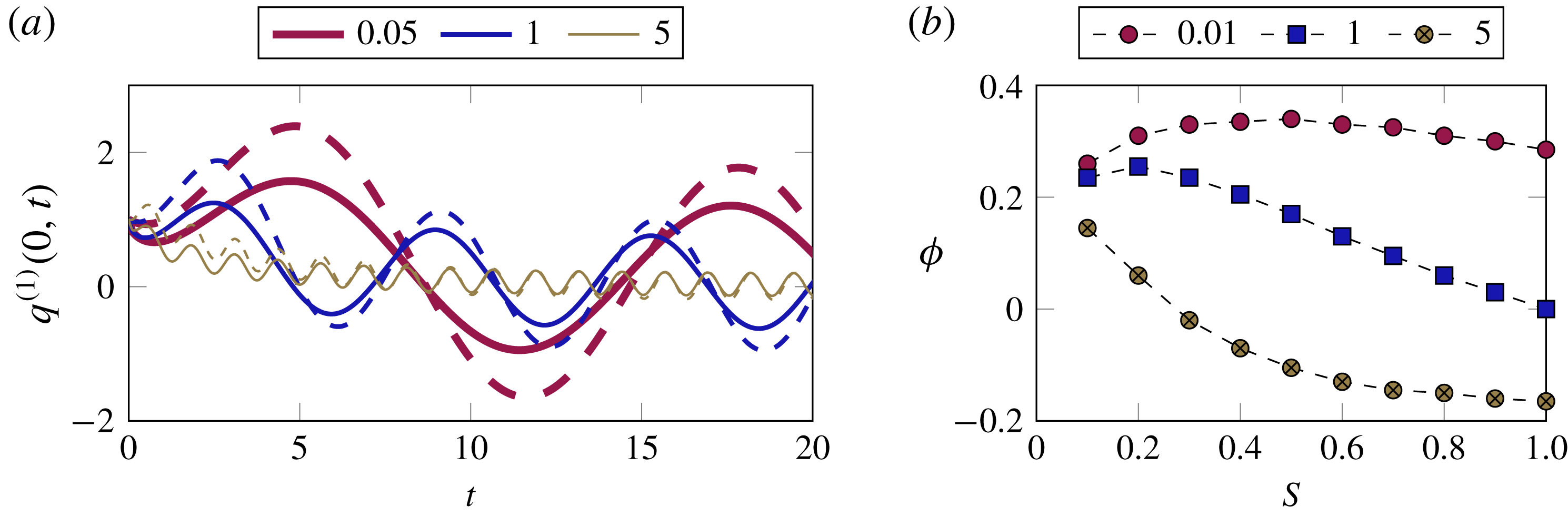
We evaluate this velocity expression as a function of time in figure 7(a) and find that, with Basset history, particles oscillate with smaller amplitudes at early time, and that they attain their final periodic state faster than when Basset history is neglected. This behaviour, governed by the short-time dynamics, is qualitatively different from that of the cases we studied in earlier sections, where Basset history significantly slowed down the attainment of terminal velocity. In particular, the Basset history integral is not simply an additional drag. We see that expressions (4.13) and (4.14) asymptote to similar expressions, albeit with a phase difference. We can quantify the phase difference
 $\unicode[STIX]{x1D719}$
that persists at long times between a particle with history effects and with only Stokes drag at long times. This is shown in figure 7(b) for Stokes number in the range
 $S=0.1$
–1 and for three different density ratios,
 $\unicode[STIX]{x1D6FD}=0.01,1,5$
. We should however remind ourselves that, though we have chosen
 $\unicode[STIX]{x1D706}\sim O(1)$
where particle relaxation time scale and forcing are similar, the solution expression is general and applies to all scenarios with frequencies capped by the diffusive time scale.
(a) Particle velocity relative to oscillating background flow when
 $\unicode[STIX]{x1D6FD}=5$
,
 $S=1$
for three different oscillating frequencies,
 $\unicode[STIX]{x1D706}=0.5,1,5$
. The dashed lines correspond to the solution with Stokes drag alone, and the solid line accounts for Basset history as well, from (4.13). (b) Phase difference
 $\unicode[STIX]{x1D719}$
between solutions including and excluding history effects as a function of Stokes number,
 $S$
, for a fixed
 $\unicode[STIX]{x1D706}=1$
and three density ratios,
 $\unicode[STIX]{x1D6FD}=0.01,1,5$
.

5 Spatially dependent flows
Thus far we considered the MR equation with spatially uniform fluid flows. When the fluid flow varies in space, the MR equation is generically nonlinear and one does not obtain a closed-form expression for the particle velocity
 $\boldsymbol{q}(0,t)$
. Most fluid flows are indeed spatially dependent. The role of the Basset history integral in determining the dynamics of inertial particles in such fluid flows has been investigated by others (Daitche & Tél Reference Daitche and Tél2011, Reference Daitche and Tél2014; Olivieri et al.
Reference Olivieri, Picano, Sardina, Iudicone and Brandt2014; Daitche Reference Daitche2015; Guseva, Daitche & Tél Reference Guseva, Daitche and Tél2017). These studies focused on the contribution of the Basset history to particle collision rates, preferential concentration and residence time of heavy/light particles. All of the aforementioned studies employed the numerical scheme developed in Daitche (Reference Daitche2013) which approximates the singular kernel of the Basset history integral. In this section, we show how our reformulation of the MR equation may be readily adapted to the case of spatially dependent fluid flows. We emphasise that no approximations are made in handling the singular kernel. Furthermore, the memory costs are constant in time.
We begin the discussion in § 5.1 by considering the dynamics of a particle in planar Couette flow. Since the fluid velocity is linear in the spatial variable, this spatially dependent problem is in fact exactly solvable. Moreover, the exact solution found here may be used to simulate the dynamics of particles in more complicated, but slowly varying, flow fields by using the leading-order term in a gradient expansion of the fluid velocity.
Our next example, in § 5.2, is that of a particle in the neighbourhood of a point vortex. Here we probe the effect of the history integral on caustics formation and also the large-time behaviour of the particle. This requires some modification of our original method to handle nonlinear forcing functions, which we describe in detail below. The extension of the numerical method, presented in this section, to cases where the fluid velocity is not specified explicitly is straightforward, though not the topic of the present paper. It is thus our contention that the numerical method we develop here is directly applicable for including the history integral in any general flow.
5.1 Example 4: migration in plane Couette flow
The Couette flow velocity profile is given by
 $u^{(1)}=\unicode[STIX]{x1D706}y^{(2)}$
. As before, the superscripts
 $(\cdot )^{(1)}$
and
 $(\cdot )^{(2)}$
represent the horizontal and vertical components, respectively. The particle velocity evolution in such a background flow is given by
 $$\begin{eqnarray}\displaystyle \unicode[STIX]{x2202}_{t}\left[\begin{array}{@{}c@{}}q^{(1)}(0,t)\\ q^{(2)}(0,t)\end{array}\right]=\underbrace{\left[\begin{array}{@{}cc@{}}\unicode[STIX]{x1D6FC} & \unicode[STIX]{x1D706}\\ 0 & \unicode[STIX]{x1D6FC}\end{array}\right]}_{\mathbb{M}}\left[\begin{array}{@{}c@{}}q^{(1)}(0,t)\\ q^{(2)}(0,t)\end{array}\right]+\unicode[STIX]{x1D6FE}\underbrace{\left[\begin{array}{@{}cc@{}}1 & 0\\ 0 & 1\end{array}\right]}_{\mathbb{I}}\left[\begin{array}{@{}c@{}}q_{x}^{(1)}(0,t)\\ q_{x}^{(2)}(0,t)\end{array}\right]. & & \displaystyle\end{eqnarray}$$
Since the boundary condition is linear with constant coefficients, we may follow a similar procedure as earlier. We now have two diffusion equations coupled at an interface, where the interfacial boundary condition in each is given by the MR equation (3.6). Note, however, that the diffusion equations themselves (i.e. in the bulk) are decoupled from each other. As a result, the global relation for this system of diffusion equations is just the vector version of (2.13):
 $$\begin{eqnarray}\displaystyle \text{e}^{\unicode[STIX]{x1D714}(k)T}\hat{\boldsymbol{q}}(k,T)+\boldsymbol{g}_{1}(k,T)+\text{i}k\boldsymbol{g}_{0}(k,T)=0,\quad k\in \mathbb{C}^{-}. & & \displaystyle\end{eqnarray}$$
The boundary condition becomes
 $$\begin{eqnarray}\displaystyle (\boldsymbol{q}(0,T)\text{e}^{\unicode[STIX]{x1D714}T}-\boldsymbol{q}(0,0))-k^{2}\boldsymbol{g}_{0}(k,T)=-\mathbb{M}(\unicode[STIX]{x1D6FC},\unicode[STIX]{x1D6FE},\unicode[STIX]{x1D706})\boldsymbol{g}_{0}(k,T)+\unicode[STIX]{x1D6FE}\boldsymbol{g}_{1}(k,T). & & \displaystyle\end{eqnarray}$$
Eliminating
 $\boldsymbol{g}_{1}(k,T)$
just as earlier from the above equation, we get for
 $\boldsymbol{g}_{0}(k,T)$
 $$\begin{eqnarray}\displaystyle ((k^{2}-\text{i}k\unicode[STIX]{x1D6FE})\mathbb{I}-\mathbb{M}(\unicode[STIX]{x1D6FC},\unicode[STIX]{x1D6FE},\unicode[STIX]{x1D706}))\boldsymbol{g}_{0}(k,T)=\{\boldsymbol{q}(0,T)\text{e}^{\unicode[STIX]{x1D714}T}-\boldsymbol{q}(0,0)+\unicode[STIX]{x1D6FE}\hat{\boldsymbol{q}}(k,T)\text{e}^{\unicode[STIX]{x1D714}T}\}, & & \displaystyle\end{eqnarray}$$
where
 $$\begin{eqnarray}\displaystyle ((k^{2}-\text{i}k\unicode[STIX]{x1D6FE})\mathbb{I}-\mathbb{M}(\unicode[STIX]{x1D6FC},\unicode[STIX]{x1D6FE},\unicode[STIX]{x1D706}))^{-1}=\left[\begin{array}{@{}cc@{}}(k^{2}-\unicode[STIX]{x1D6FC}-\text{i}k\unicode[STIX]{x1D6FE})^{-1} & \unicode[STIX]{x1D706}(k^{2}-\unicode[STIX]{x1D6FC}-\text{i}k\unicode[STIX]{x1D6FE})^{-2}\\ 0 & (k^{2}-\unicode[STIX]{x1D6FC}-\text{i}k\unicode[STIX]{x1D6FE})^{-1}\end{array}\right]. & & \displaystyle\end{eqnarray}$$
Multiplying the above equation by
 $\text{i}k\text{e}^{-k^{2}t}$
and integrating over
 $\unicode[STIX]{x2202}{\mathcal{D}}^{-}$
we obtain the solution
 $$\begin{eqnarray}\displaystyle \unicode[STIX]{x03C0}\boldsymbol{q}(0,t)=-\int _{-\infty }^{\infty }\text{i}k\text{e}^{-k^{2}t}\left[\begin{array}{@{}cc@{}}(k^{2}-\unicode[STIX]{x1D6FC}-\text{i}k\unicode[STIX]{x1D6FE})^{-1} & \unicode[STIX]{x1D706}(k^{2}-\unicode[STIX]{x1D6FC}-\text{i}k\unicode[STIX]{x1D6FE})^{-2}\\ 0 & (k^{2}-\unicode[STIX]{x1D6FC}-\text{i}k\unicode[STIX]{x1D6FE})^{-1}\end{array}\right]\boldsymbol{q}(0,0)\,\text{d}k. & & \displaystyle\end{eqnarray}$$
On the other hand, the solution to the MR equation without the Basset history integral simplifies to
 $$\begin{eqnarray}\displaystyle \boldsymbol{q}(0,t)=\text{e}^{-\unicode[STIX]{x1D6FC}t}\left[\begin{array}{@{}cc@{}}1 & -\unicode[STIX]{x1D706}t\\ 0 & 1\end{array}\right]\boldsymbol{q}(0,0). & & \displaystyle\end{eqnarray}$$
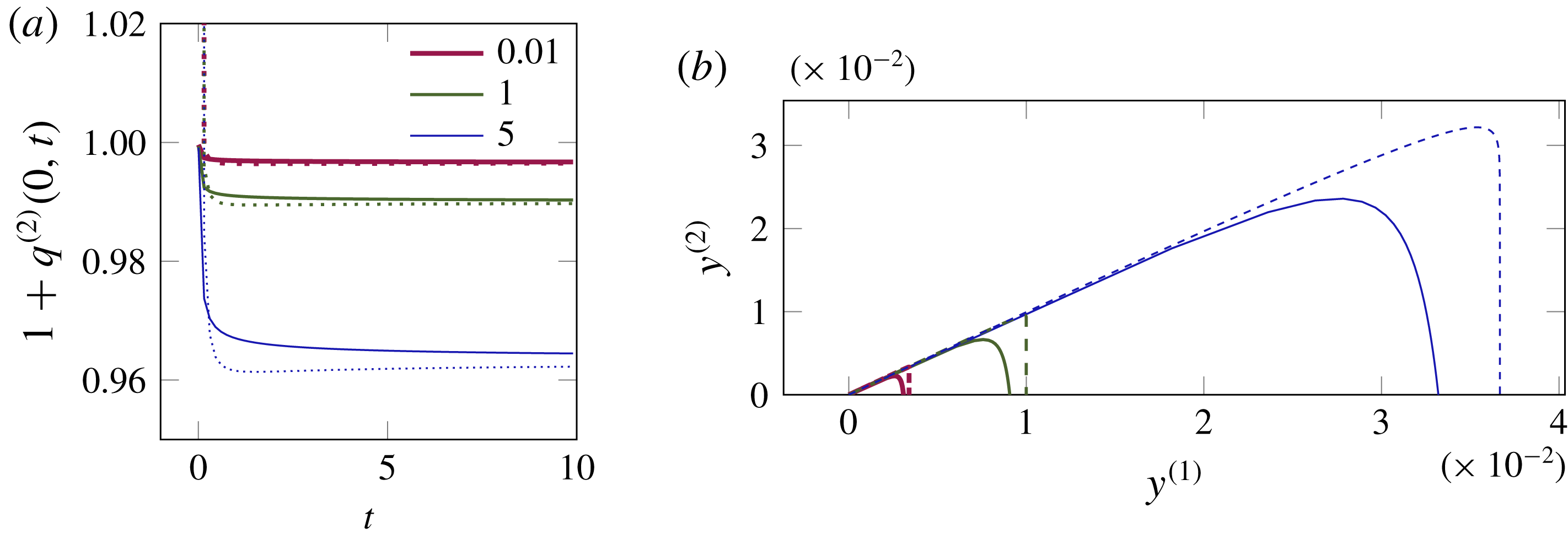
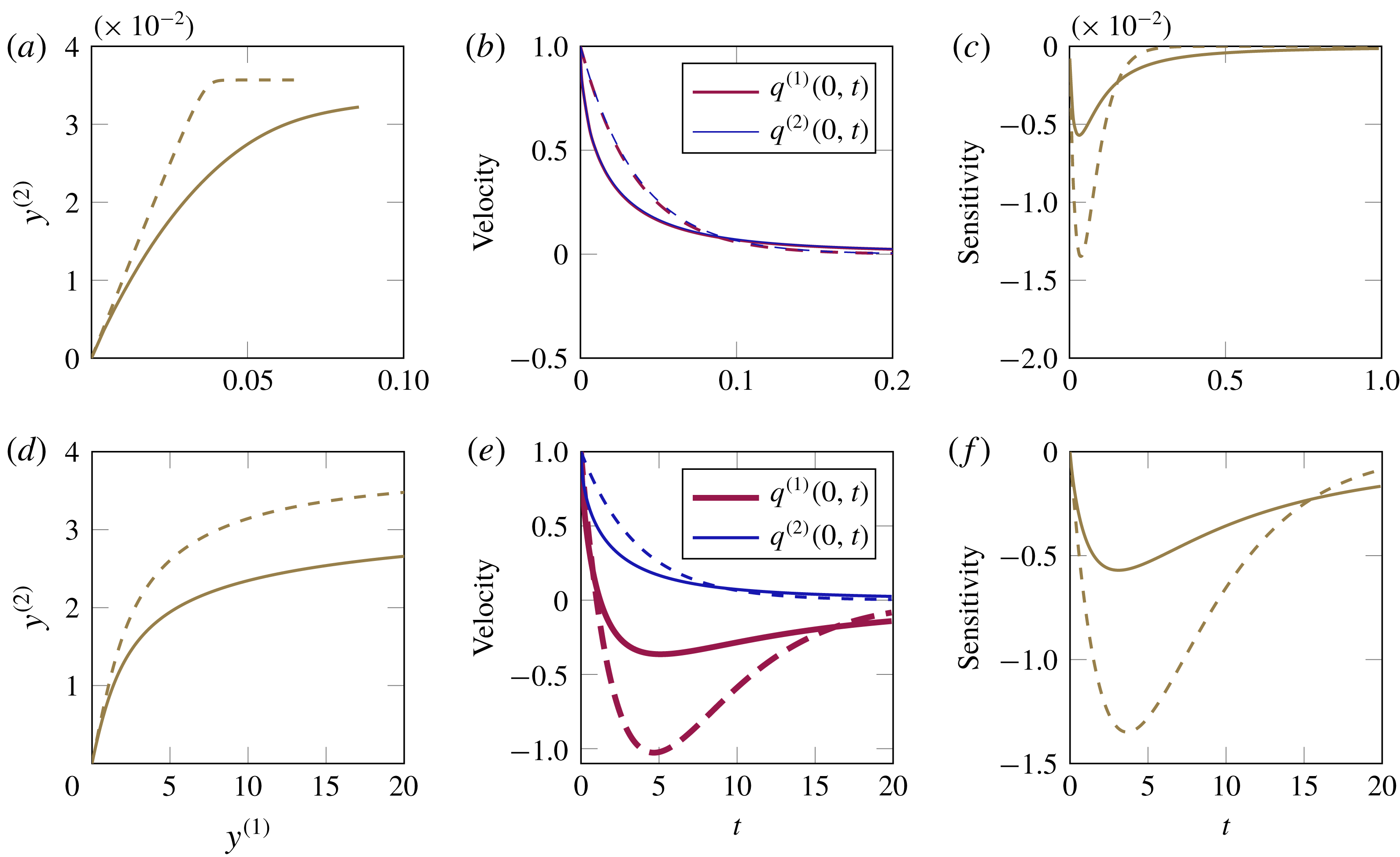
The results are provided in figure 8. Figure 8(a) and (d), respectively, for Stokes number
 $S=0.01$
and 1, show particle trajectories with and without Basset history. The
 $y^{(2)}$
coordinate has saturated to the values shown. Clearly the migratory behaviour is different, and neglecting Basset history predicts the final locations of the particles incorrectly. Furthermore, the relaxation time is longer with Basset history, i.e. the velocity decay is slower, as seen in figure 8(b,e). Note that the relative velocity is plotted here, so each particle at long time attains the local velocity of the Couette flow (
 $=\unicode[STIX]{x1D706}y^{(2)}$
). The solution expressions (5.6)–(5.7) readily lead to the following expressions for the sensitivity of the solution to a particle’s initial velocity:
 $$\begin{eqnarray}\displaystyle & \displaystyle \left(\frac{\unicode[STIX]{x1D6FF}\boldsymbol{q}(0,t)}{\unicode[STIX]{x1D6FF}\boldsymbol{q}(0,0)}\right)_{His}=-\frac{1}{\unicode[STIX]{x03C0}}\int _{-\infty }^{\infty }\text{i}k\text{e}^{-k^{2}t}\left[\begin{array}{@{}cc@{}}(k^{2}-\unicode[STIX]{x1D6FC}-\text{i}k\unicode[STIX]{x1D6FE})^{-1} & \unicode[STIX]{x1D706}(k^{2}-\unicode[STIX]{x1D6FC}-\text{i}k\unicode[STIX]{x1D6FE})^{-2}\\ 0 & (k^{2}-\unicode[STIX]{x1D6FC}-\text{i}k\unicode[STIX]{x1D6FE})^{-1}\end{array}\right]\,\text{d}k, & \displaystyle\end{eqnarray}$$
 $$\begin{eqnarray}\displaystyle & \displaystyle \left(\frac{\unicode[STIX]{x1D6FF}\boldsymbol{q}(0,t)}{\unicode[STIX]{x1D6FF}\boldsymbol{q}(0,0)}\right)_{Sto}=\text{e}^{-\unicode[STIX]{x1D6FC}t}\left[\begin{array}{@{}cc@{}}1 & -\unicode[STIX]{x1D706}t\\ 0 & 1\end{array}\right]. & \displaystyle\end{eqnarray}$$
The eigenvalues of this sensitivity matrix provide the Lyapunov exponents, and both eigenvalues are equal to 1 for the scenarios with and without Basset history. However, the eigenvectors corresponding to these matrices are different and in figure 8(c,f) we plot the evolution of the off-diagonal component for two different
 $S=0.01,1$
.
Particle dynamics in Couette flow. Solid lines are the solutions in (5.6), while dashed lines indicate dynamics upon neglecting Basset history in (5.7). (a–c) Corresponds to solution for
 $S=0.01$
and (d–f) for
 $S=1$
for a fixed density ratio of
 $\unicode[STIX]{x1D6FD}=5$
. (a,d) Horizontal component
 $q^{(1)}(0,t)$
and vertical component
 $q^{(2)}(0,t)$
, respectively, of particle velocity relative to fluid velocity with initial velocity of particle relative to fluid
 $\boldsymbol{q}(0,0)=1$
. (b,e) Particle trajectory as a function of time. We see that the particle velocity is the same in both directions, however decaying differently. (c,f) Off-diagonal component of sensitivity matrix in (5.9) which is due to shear in the flow.

5.2 Solution for nonlinear spatial flows
So far, we have been able to explicitly compute the particle velocity, from
 $\tilde{\boldsymbol{g}}_{0}(\unicode[STIX]{x1D714},T)$
; see (3.14). However, when the spatial dependence of the fluid flow is nonlinear, i.e. when
 $\boldsymbol{f}$
depends on
 $\boldsymbol{y}$
, equation (3.14) is not an explicit expression for the particle velocity. Consequently we resort to a numerical scheme to evolve the dynamics of the particle, which we present in this section. Our numerical method has the following advantages:
(i) The method completely eliminates the need to store the entire trajectory of the particle to evaluate the Basset history term.
(ii) Our method achieves spectral accuracy by employing Chebyshev polynomials to evaluate the integrals involved.
(iii) The method involves a fixed memory cost (of
$O(N)$
,
$N$
being the number of Chebyshev modes) independent of time, making long-time simulations no more expensive than short-time ones. This is useful to compute statistics in turbulent simulations.(iv) The effect of history can be recorded (with fixed memory size), enabling simulations to be restarted. Such a restart is impossible in other techniques owing to exponentially large memory costs in evaluating the integral. While preparing the paper we became aware of the work of Parmar et al. (Reference Parmar, Annamalai, Balachandar and Prosperetti2018) who approximate the history kernel by a summation of exponentials and achieve the desired accuracy. However, we would like to highlight that our technique does not make any approximation to the kernel and we show later that all information due to history can be stored in a variable whose computation is of fixed memory throughout particle evolution. Moreover, the form of the solution in (3.16) is specially useful for studying asymptotic behaviour (authors’ work in preparation), unlike other techniques.


In the following subsection we derive the equations we ultimately solve for the particle trajectory and in the subsequent subsection we provide the details of the numerical implementation.
5.2.1 Evolution equation for Basset history integral
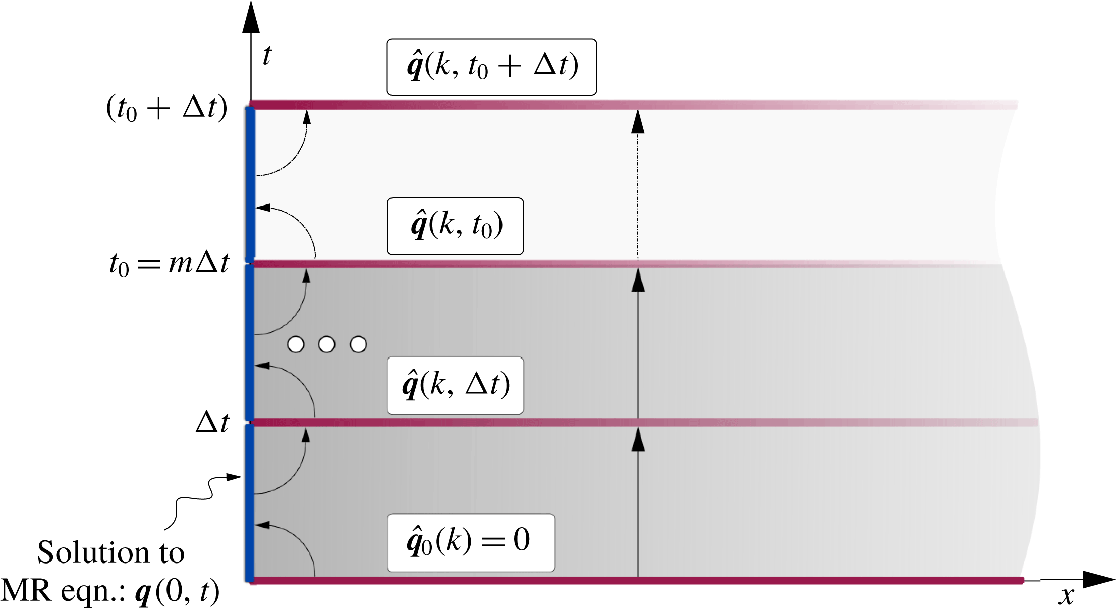
Schematic showing numerical scheme where we evaluate
 $\hat{\boldsymbol{q}}(k,t)$
at intervals
 $t_{0},~(t_{0}+\unicode[STIX]{x0394}t)$
from the solution at
 $t\in [t_{0}-\unicode[STIX]{x0394}t,t_{0}],~[t_{0},t_{0}+\unicode[STIX]{x0394}t]$
and so on in order to eliminate the need to store
 $\boldsymbol{q}(0,t)$
from
 $t\in [0,t_{0}+\unicode[STIX]{x0394}t]$
.

We begin by dividing the
 $x$
–
 $t$
plane into domains of size
 $[0,\infty )\times [t_{0}-\unicode[STIX]{x0394}t,t_{0}]$
, where
 $t_{0}=m\unicode[STIX]{x0394}t$
for some integer
 $m$
, as shown in figure 9. Our procedure involves two steps, repeated for each such domain:
(1) Using the initial condition
$\boldsymbol{q}(x,t_{0}-\unicode[STIX]{x0394}t)$
in each domain (bottom wall of that domain in figure 9), we compute the boundary condition
$\boldsymbol{q}(0,t),~t\in (t_{0}-\unicode[STIX]{x0394}t,t_{0}]$
(left wall of that domain). This is done by solving the MR equation in the form given by (5.11) below. This equation is the extension of (3.16) to the case of arbitrary initial conditions. Moreover, the forcing
$\boldsymbol{f}$
is now a function of
$\boldsymbol{q}(0,t)$
and/or
$\boldsymbol{y}(t)$
. So we start with a guess for
$\boldsymbol{q}(0,t)$
and
$\boldsymbol{y}(t)$
, and iterate using a nonlinear solver. We thus have the Dirichlet condition on the left wall of figure 9, over
$[t_{0}-\unicode[STIX]{x0394}t,t_{0}]$
.(2) Using the computed boundary condition
$\boldsymbol{q}(0,t)$
from the previous step and the known initial condition
$\boldsymbol{q}(x,t_{0}-\unicode[STIX]{x0394}t)$
, we directly compute
$\boldsymbol{q}(x,t_{0})$
, the top wall of that domain, by using (5.13), which will be derived below. This step is equivalent to solving the diffusion equation with a Dirichlet boundary condition, and the solution of this boundary-value problem leads to the initial condition for the next domain,
$t\in (t_{0},t_{0}+\unicode[STIX]{x0394}t]$
. Through an efficient use of the global relation, we do not require the explicit solution expression
$\boldsymbol{q}(x,t_{0})$
, but only the Fourier transform
$\hat{\boldsymbol{q}}(k,t_{0})$
, which simplifies the calculations considerably.


We recognise that our system size (namely, the number of dependent variables) is higher for a nonlinear case, and this is the price we need to pay to eliminate the rising memory costs coming from the non-local time integral term.
In the first domain alone
 $[0,\infty )\times [0,\unicode[STIX]{x0394}t]$
, equation (3.16) may be used to obtain the particle velocity. We recognise that
 $\boldsymbol{f}$
now depends on
 $\boldsymbol{y}$
and
 $\boldsymbol{q}(0,t)$
. Along with (3.7), where we set
 $T=\unicode[STIX]{x0394}t$
, we now have two equations for two unknowns,
 $\boldsymbol{y}$
and
 $\boldsymbol{q}(0,t)$
, over the time interval
 $[0,\unicode[STIX]{x0394}t]$
. In a standard numerical method, one would approximate the first integral of (3.16) using a quadrature rule. We, however, adopt an alternative route (partly to ensure accuracy) by representing the unknowns
 $\boldsymbol{q}(0,t)$
and
 $\boldsymbol{y}(t)$
in terms of Chebyshev polynomials over the interval
 $[0,\unicode[STIX]{x0394}t]$
. All integrals are readily evaluated to a high degree of accuracy. With the Chebyshev polynomial representation, equations (3.16) and (3.7) are solved using a nonlinear solver, here Newton’s method, for the coefficients of the Chebyshev polynomials. Once we have
 $\boldsymbol{q}(0,t)$
(in terms of Chebyshev polynomials), we solve the diffusion equation with this Dirichlet condition to obtain the solution
 $\boldsymbol{q}(x,\unicode[STIX]{x0394}t)$
. The evaluation of such new initial conditions at every
 $(t_{0}=m\unicode[STIX]{x0394}t)$
is possible precisely because of the relationship between the Basset history integral and the Neumann condition to the diffusion equation.
In all later domains, the initial condition
 $\boldsymbol{q}(x,t_{0})$
is no longer zero. Indeed
 $\boldsymbol{q}(x,t_{0})$
is the solution of the diffusion equation at this time. The global relation of the diffusion equation in the time interval
 $t\in (t_{0},t_{0}+\unicode[STIX]{x0394}t]$
can be written as
 $$\begin{eqnarray}\displaystyle & & \displaystyle \text{e}^{k^{2}(t_{0}+\unicode[STIX]{x0394}t)}\hat{\boldsymbol{q}}(k,(t_{0}+\unicode[STIX]{x0394}t))\nonumber\\ \displaystyle & & \displaystyle \quad =\text{e}^{k^{2}t_{0}}\hat{\boldsymbol{q}}(k,t_{0})-\text{i}k\tilde{\boldsymbol{g}}_{0}(k^{2},t_{0},t_{0}+\unicode[STIX]{x0394}t)-\tilde{\boldsymbol{g}}_{1}(k^{2},t_{0},t_{0}+\unicode[STIX]{x0394}t),\quad k\in \mathbb{C}^{-}.\end{eqnarray}$$
For the boundary terms represented by
 $\tilde{\boldsymbol{g}}_{i}(k^{2},t_{1},t_{2})$
, we have introduced the additional arguments
 $t_{1}$
and
 $t_{2}$
, which are the limits of the integral defining the time transform. This notation is also used in the forcing, as
 $\tilde{\boldsymbol{f}}(k^{2},t_{1},t_{2})$
. Following a procedure similar to that employed to derive (3.14), we obtain the following expression for
 $\boldsymbol{q}(0,t)$
 $$\begin{eqnarray}\displaystyle -\frac{\unicode[STIX]{x03C0}}{2}\boldsymbol{q}(0,t) & = & \displaystyle \underbrace{\int _{0}^{\infty }k\text{e}^{-k^{2}(t-t_{0})}\text{Im}\{\mathscr{H}(k,t_{0})\}\,\text{d}k}_{{\mathcal{H}}(t)}\nonumber\\ \displaystyle & & \displaystyle +\,\underbrace{\int _{0}^{\infty }\text{Im}\left\{\frac{k\text{e}^{-k^{2}t}\tilde{\boldsymbol{f}}(k^{2},t_{0},t)}{\unicode[STIX]{x1D6FC}-k^{2}+\text{i}k\unicode[STIX]{x1D6FE}}\right\}\,\text{d}k}_{{\mathcal{F}}(t)},\quad t\in (t_{0},t_{0}+\unicode[STIX]{x0394}t].\end{eqnarray}$$
The term
 $\mathscr{H}(k,t_{0})$
in the integrand of the first integral in the expression above is the modified initial condition given by
 $$\begin{eqnarray}\displaystyle \mathscr{H}(k,t_{0})=\left\{\frac{\boldsymbol{q}(0,t_{0})+\unicode[STIX]{x1D6FE}\hat{\boldsymbol{q}}(k,t_{0})}{\unicode[STIX]{x1D6FC}-k^{2}+\text{i}k\unicode[STIX]{x1D6FE}}\right\}. & & \displaystyle\end{eqnarray}$$
This term encodes all the information about the history of the particle from
 $t\in (0,t_{0}]$
. Equation (5.11) is thus the extension of (3.16) for a general initial condition to the diffusion equation. The renormalised initial condition
 $\mathscr{H}(k,t)$
itself evolves in time and this evolution is once again obtained from the global relation; see appendix B for details. We state the relevant equation here:
 $$\begin{eqnarray}\displaystyle \mathscr{H}(k,t_{0})=\text{e}^{-k^{2}\unicode[STIX]{x0394}t}\mathscr{H}(k,t_{0}-\unicode[STIX]{x0394}t)-\underbrace{\text{e}^{-k^{2}t_{0}}\int _{t_{0}-\unicode[STIX]{x0394}t}^{t_{0}}\text{e}^{k^{2}s}\boldsymbol{q}(0,s)\,\text{d}s}_{\mathscr{I}_{1}}-\underbrace{\text{e}^{-k^{2}t_{0}}\frac{\,\tilde{\boldsymbol{f}}(k^{2},t_{0}-\unicode[STIX]{x0394}t,t_{0})}{\unicode[STIX]{x1D6FC}-k^{2}+\text{i}k\unicode[STIX]{x1D6FE}}}_{\mathscr{I}_{2}}. & & \displaystyle \nonumber\\ \displaystyle & & \displaystyle\end{eqnarray}$$
Note that all terms on the right-hand side of (5.13), including the forcing term, are known since they depend on the previous time interval
 $[t_{0}-\unicode[STIX]{x0394}t,t_{0}]$
. Equation (5.13) may also be written as a dynamical system for individual modes of history as
 $$\begin{eqnarray}\displaystyle \dot{\mathscr{H}}(k,t)+k^{2}\mathscr{H}(k,t)=\boldsymbol{q}(0,t)+\frac{\,\boldsymbol{f}(t,\boldsymbol{y}(t),\boldsymbol{q}(0,t))}{\unicode[STIX]{x1D6FC}-k^{2}+\text{i}k\unicode[STIX]{x1D6FE}},\quad t\in [t_{0}-\unicode[STIX]{x0394}t,t_{0}]. & & \displaystyle\end{eqnarray}$$
Equations (5.11) and (5.13) represent the solution to the full MR equations for a particle in a time-dependent inhomogeneous flow field. Note that the individual modes
 $k$
of
 $\mathscr{H}(k,t)$
in (5.13) evolve independently. However, the expression for the velocity in (5.11) depends on all of them, and indeed depends on the integral of the history.
We are now enabled to march repeatedly till any
 $t_{0}$
from any
 $(t_{0}-\unicode[STIX]{x0394}t)$
using the set of initial conditions
 $\hat{\boldsymbol{q}}(k,t_{0}-\unicode[STIX]{x0394}t)$
, solving equation (5.11) for
 $\boldsymbol{y}(t)$
and
 $\boldsymbol{q}(0,t)$
in the interval
 $(t_{0}-\unicode[STIX]{x0394}t)$
to
 $t_{0}$
, and using these Dirichlet boundary conditions in (5.13) to get
 $\hat{\boldsymbol{q}}(k,t_{0})$
. Once again, we emphasise that the above procedure eliminates the need to store the entire particle velocity from the initial time instant. The effect of the Basset history integral is encoded in
 $\mathscr{H}(k,t)$
.
5.3 Numerical technique
We now detail a numerical scheme to solve equations (5.11)–(5.13). The continuous variables
 $t$
and
 $k$
are restricted to a set of discrete values over their respective intervals,
 $t\in (t_{0}-\unicode[STIX]{x0394}t,t_{0}]$
and
 $k\in [0,\infty )$
, leading to discrete times
 $t_{j}$
and discrete wavenumbers
 $k_{l}$
where
 $j=1,\ldots ,L$
and
 $l=0,\ldots ,N$
. In the case of
 $t$
we employ Chebyshev nodes under an affine transform, whereas for
 $k$
we employ a mapped Chebyshev node appropriate for rational Chebyshev approximations. We then expand
 $\boldsymbol{q}(0,t)$
and
 $\mathscr{H}(k,t_{0})$
in a Chebyshev polynomial basis
 $T_{n}(t)$
(rational Chebyshev polynomials for
 $\mathscr{H}$
). We adopt a collocation approach to solve the resulting nonlinear equation.
The discrete version of (5.11) can be written as a nonlinear equation for the coefficients as
 $$\begin{eqnarray}\displaystyle \mathscr{T}(t_{j})\equiv \frac{\unicode[STIX]{x03C0}}{2}\boldsymbol{q}(0,t_{j})+{\mathcal{H}}(t_{j})+{\mathcal{F}}(t_{j})=0,\quad t_{j}=t_{0}+\frac{\unicode[STIX]{x0394}t}{2}\left(1+\cos \left(\frac{j\unicode[STIX]{x03C0}}{L}\right)\right), & & \displaystyle\end{eqnarray}$$
where
 $j=1,\ldots ,L$
. Details on how to compute each term in the above equation are presented in appendix C. The contribution from
 $\mathscr{H}(k,t_{0})$
is captured in
 ${\mathcal{H}}(t_{j})$
, whereas the contribution from the nonlinear forcing due to the fluid velocity field is present in
 ${\mathcal{F}}(t_{j})$
. An equation for the position
 $\boldsymbol{y}$
can be obtained from the discretised version (3.7). A standard Newton root finder is employed to solve for
 $\boldsymbol{q}(0,t)$
and
 $\boldsymbol{y}(t)$
in the time interval
 $(n\unicode[STIX]{x0394}t,(n+1)\unicode[STIX]{x0394}t]$
for each
 $n=0,1,\ldots$
with an appropriate initial guess, typically
 $\boldsymbol{q}(0,t_{j})=-2/\unicode[STIX]{x03C0}{\mathcal{H}}(t_{j})$
. Equation (5.13) on the other hand is a straightforward integral evaluation using known values of
 $\boldsymbol{q}(0,t_{j})$
and
 $\mathscr{H}(k_{j},t_{0}-\unicode[STIX]{x0394}t)$
from the previous time step. We show in the appendix that expanding
 $\boldsymbol{q}(0,t)$
and
 $\mathscr{H}(k,t_{0}-\unicode[STIX]{x0394}t)$
in Chebyshev basis allows us to precompute several terms, which speeds up evaluation of expressions in (5.13).
Error estimates for the solution to a relaxing particle using the numerical scheme developed in § 5.3. Error as a function of time for (a) different values of
 $N$
at fixed
 $L=20$
and (c) different values of
 $L$
at fixed
 $N=50,70$
. (b,d) Maximum of the error as we increase the number of Chebyshev modes in
 $k$
and
 $t$
.

5.4 Convergence properties and memory requirement of the numerical scheme
To study convergence of our numerical scheme, we compare the exact velocity of a relaxing particle (for which we have an analytic expression) to the numerical solution obtained from the scheme described above. We first check the numerical method’s accuracy as a function of the number of Chebyshev nodes
 $N$
in wavenumber
 $\tilde{k}$
, where
 $\tilde{k}:~k\in [0,\infty ]\rightarrow [-1,1]$
. We also check the accuracy for number of Chebyshev nodes
 $L$
in
 $t\in [t_{0},t_{0}+\unicode[STIX]{x0394}t]$
within a time interval of length
 $\unicode[STIX]{x0394}t$
. The error in the calculated solution is given by
 $$\begin{eqnarray}\displaystyle \mathscr{E}(t_{j})=|q^{(1)}(0,t_{j})-q_{e}^{(1)}(0,t_{j})|, & & \displaystyle\end{eqnarray}$$
where
 $q_{e}^{(1)}(0,t_{j})$
is the exact solution evaluated at discrete
 $t_{j}$
and
 $q^{(1)}(0,t_{j})$
is the solution evaluated using the present numerical technique. In figure 10(a) we plot the error as a function of time for all the number of
 $\tilde{k}$
chosen and we see its magnitude decrease with increase in
 $N$
. In figure 10(b) we plot the maximum value of
 $\mathscr{E}(t_{j})$
. We clearly see that the error is small and decreases exponentially with increase in
 $N$
for fixed
 $L=20$
. We can reach a desired accuracy by choosing the appropriate number of Chebyshev nodes
 $N$
. Moving now to the convergence of the solution with increase in nodes
 $L$
in
 $\unicode[STIX]{x0394}t$
, we see there is a general increase in error in figure 10(d) for both fixed
 $N=50$
and 70. Such a behaviour is expected and not an anomaly. Firstly observe that the maximum error is attained, for all different values of
 $L$
and
 $N$
, at the first grid point, i.e.
 $t_{1}$
in
 $t_{j}\in (0,\unicode[STIX]{x0394}t]$
. This is because of the
 $t^{-1/2}$
singularity at
 $t=0$
. As we increase the number of Chebyshev nodes in the interval of length
 $\unicode[STIX]{x0394}t$
, the first Chebyshev grid point moves closer to this singularity. We can easily account for this behaviour by increasing the number of modes in space
 $N$
. We show this by increasing the spatial Chebyshev modes from
 $N=50$
to 70 in figure 10(d), which results in a drop in the maximum error.
We emphasise the advantage that a Chebyshev basis provides in terms of computational efficiency. In order to compute the Chebyshev coefficients via the discrete Chebyshev transform (DCT), we only require
 $O(N\log N)$
operations, where
 $N$
is the number of Chebyshev modes. This is done by leveraging a fast Fourier transform (FFT) package to evaluate the DCTs involved in the process of computing Chebyshev coefficients.
The memory requirement for our technique comes from storing the variables
 $\boldsymbol{q}(0,t_{j})$
and
 $\mathscr{H}(k_{j},t_{0})$
. Considering
 $L$
modes in
 $t_{j}$
,
 $N$
modes in
 $\tilde{k}_{j}$
demands only storage of
 $O(N+L)$
values for all times, whereas the other techniques require a linearly increasing memory cost of
 $O(t/\unicode[STIX]{x0394}t)$
. For
 $N=30,~L=20$
, one needs to store only 50 values, which remain fixed throughout the simulation. In this estimate, of course, we do not account for the precomputed matrices, which turn out to be three
 $N\times N$
matrices (see appendix C) resulting in another 2700 values for
 $N=30$
, but this initial cost remains constant and helps in shorter computation time.
5.5 Example 5: single point vortex and caustics
The stationary flow field corresponding to a single vortex is
 $$\begin{eqnarray}\displaystyle \boldsymbol{u}=\frac{\unicode[STIX]{x1D6E4}}{2\unicode[STIX]{x03C0}}\hat{\boldsymbol{e}}_{z}\times \frac{\,\boldsymbol{y}(t)}{|\,\boldsymbol{y}|^{2}}. & & \displaystyle\end{eqnarray}$$
Though this flow field does not have a time-varying component, it still has contributions from both
 $(\boldsymbol{u}\boldsymbol{\cdot }\unicode[STIX]{x1D735})\boldsymbol{u}$
and
 $(\boldsymbol{q}(0,t)\cdot \unicode[STIX]{x1D735})\boldsymbol{u}$
. This makes the system of evolution equations for particle position
 $\boldsymbol{y}(t)$
and velocity
 $\boldsymbol{q}(0,t)$
coupled and nonlinear. The solution is given by
 $$\begin{eqnarray}\displaystyle \boldsymbol{y}(t)=\boldsymbol{y}(0)+\int _{0}^{t}\boldsymbol{q}(0,s)\,\text{d}s+\int _{0}^{t}\frac{\unicode[STIX]{x1D6E4}}{2\unicode[STIX]{x03C0}}\hat{\boldsymbol{e}}_{z}\times \frac{\,\boldsymbol{y}(s)}{|\,\boldsymbol{y}|^{2}}\,\text{d}s, & & \displaystyle\end{eqnarray}$$
for the velocity evolution
 $$\begin{eqnarray}\displaystyle \boldsymbol{q}_{t}(0,t)+\unicode[STIX]{x1D6FC}\boldsymbol{q}(0,t)-\unicode[STIX]{x1D6FE}\boldsymbol{q}_{x}(0,t)=\left(\frac{1}{R}-1\right)(\boldsymbol{u}\boldsymbol{\cdot }\unicode[STIX]{x1D735})\boldsymbol{u}-(\boldsymbol{q}(0,t)\boldsymbol{\cdot }\unicode[STIX]{x1D735})\boldsymbol{u}. & & \displaystyle\end{eqnarray}$$
Using the numerical technique described in the previous section, we solve for position and velocity for a Stokes number of
 $S=0.01$
and density ratio
 $\unicode[STIX]{x1D6FD}=20$
, and plot the radial and angular velocity in figure 11(a,b). Different lines in the figure correspond to different initial position separated by a distance of 0.15 though all particles start with an initial velocity of
 $(0.05,0.05)$
. Once the particles get centrifuged far away from the vortex, the trajectory follows
 $y^{(r)}(t)\sim t^{1/4}$
, where
 $y(r)$
is the radial distance from the point vortex. Thus the radial velocity
 $q^{(r)}(0,t)\sim t^{-3/4}$
, as in figure 11(c). This long-time behaviour is the same as that obtained by Ravichandran & Govindarajan (Reference Ravichandran and Govindarajan2015) without Basset history. The history integral affects the transient behaviour and the approach to the long-time limit.
(a) Radial velocity, (b) angular velocity and (c) radial distance travelled by particles starting at five different locations separated by a non-dimensional distance of 0.15 at
 $S=0.01$
and
 $\unicode[STIX]{x1D6FD}=10$
, with an initial velocity of
 $\boldsymbol{v}_{0}=(0.05,0.05)$
and
 $\unicode[STIX]{x1D6E4}=2\unicode[STIX]{x03C0}$
. The solid black lines correspond to power laws of
 $t^{-3/4}$
or
 $t^{1/4}$
, as marked. Solid coloured lines represent simulations including the Basset history integral, Stokes drag and added-mass effects, while the dashed coloured lines are for Stokes drag with added mass.

We discussed in the introduction about caustics near a vortex. As shown analytically by Ravichandran & Govindarajan (Reference Ravichandran and Govindarajan2015), and in 2-D simulations of turbulence, particles inside a critical radius
 $r_{c}$
are evacuated rapidly, resulting in a region of high particle concentration in the neighbourhood of
 $r_{c}$
. In order to identify this critical radius, including the effects of Basset history, we track the radial separation
 $\unicode[STIX]{x0394}r$
between two particles that are initially placed close to each other. This is shown in figure 12(a) for various initial radial distances
 $r_{i}$
from the vortex of the inner particle (the one closer to the vortex). When
 $\unicode[STIX]{x0394}r$
crosses zero, caustics have occurred. We find that caustics occur for
 $r_{i}\leqslant 0.44$
, i.e.
 $r_{c}=0.44$
, for this Stokes number
 $S=0.02$
. Also, the trajectories of particles that exhibit caustics take different paths compared to ones that do not, in the phase plane defined by
 $\unicode[STIX]{x0394}v_{r}$
versus
 $\unicode[STIX]{x0394}r$
, where
 $\unicode[STIX]{x0394}v_{r}$
is the difference in radial velocities for two closely placed particles (see Ravichandran & Govindarajan Reference Ravichandran and Govindarajan2015). This is shown in figure 12(b), where a negative value of
 $\unicode[STIX]{x0394}v_{r}$
implies that the inner particle travels faster than its neighbour. When
 $\unicode[STIX]{x0394}r$
becomes negative it has overtaken its neighbour. Thus trajectories that cross the
 $y$
-axis of the phase plane form caustics.
In figure 12(c) we plot the critical radius
 $r_{c}$
(found from the location where
 $\min (\unicode[STIX]{x0394}r(t))=0$
) as a function of the Stokes number
 $S$
. Simulations with history integral and added-mass effects included are shown as solid lines and with just Stokes drag as dotted lines. The history integral and added mass together reduce the region over which caustics are formed, and may cause a reduction in the number densities of particles predicted without the history term. The implications for particle dynamics in turbulent fluid flows are beyond the realm of the present article and will be explored in our upcoming study.
(a) Evolution of the difference in radial distance between particles
 $\unicode[STIX]{x0394}r$
for different initial particle locations
 $r_{i}$
separated by a distance
 $0.05$
for Stokes number
 $S=0.02$
. The critical particle location at which
 $\min (\unicode[STIX]{x0394}r)$
crosses the
 $t$
-axis is the location of the end of caustic formation. (b) The phase portrait defined by
 $\unicode[STIX]{x0394}v_{r}$
, the difference in radial velocity versus
 $\unicode[STIX]{x0394}r$
, also shows the transition from caustic formation to no caustic formation with increase in
 $r_{i}$
. (c) Critical radius
 $r_{c}$
for caustic formation as a function of Stokes number
 $S$
with history integral, added mass (solid line) and with Stokes drag alone (dashed line).

6 Discussion
6.1 Interpretation of the Dirichlet–Neumann map
The map that we establish between the Basset history integral and the Neumann condition of the 1-D diffusion equation arises on mathematical grounds, but can also be interpreted physically as follows. The diffusion equation that the variable
 $\boldsymbol{q}(x,t)$
obeys can be seen as diffusion of momentum from the particle boundary, and the Neumann condition
 $\boldsymbol{q}_{x}(0,t)$
on the other hand would mean the flux of momentum transferred from the particle boundary in the form of shear stress to the bulk of the fluid. The trail left by the particle motion is a consequence of this momentum flux that emanates from the particle boundary which has been shown to arise from the map between Dirichlet–Neumann conditions to diffusion equation. This relation to the diffusion or heat equation further emphasises the fact that our analysis accounts for the momentum diffusion valid before any convective inertial effects impact the ‘wake’ generated by the particle.
6.2 Different geometries
In the present paper, we have focused on our reformulation of the MR equation for spherical particles. The technique employed here is, however, general and extends immediately to other particle shapes. The only additional requirement for spheroids and disks travelling parallel to their axis of symmetry is the redefinition of the three non-dimensional quantities
 $$\begin{eqnarray}\displaystyle \hat{\unicode[STIX]{x1D6FD}}=\unicode[STIX]{x1D6FD}/\mathscr{C}_{A},\quad \hat{\unicode[STIX]{x1D6FC}}=\mathscr{C}_{a}\unicode[STIX]{x1D6FC}\quad \text{and}\quad \hat{\unicode[STIX]{x1D6FE}}=\mathscr{C}_{H}\unicode[STIX]{x1D6FE}, & & \displaystyle\end{eqnarray}$$
which respectively appear in (1.2) as coefficients to the added-mass term, the Stokes drag term and the Basset history integral. In table 1 we show how these quantities vary from those of a sphere as the aspect ratio
 $\unicode[STIX]{x1D718}$
is varied. The solution for all time-dependent spatially homogeneous flows can now be easily written for all these geometries as
 $$\begin{eqnarray}\displaystyle -\unicode[STIX]{x03C0}\boldsymbol{q}(0,t)=\int _{\unicode[STIX]{x2202}{\mathcal{D}}^{-}}\frac{\text{i}k\text{e}^{-k^{2}t}\tilde{\boldsymbol{f}}(k)}{\hat{\unicode[STIX]{x1D6FC}}-k^{2}+\text{i}k\hat{\unicode[STIX]{x1D6FE}}}\,\text{d}k-\int _{-\infty }^{\infty }\frac{\boldsymbol{v}_{0}\text{i}k\text{e}^{-k^{2}t}}{\hat{\unicode[STIX]{x1D6FC}}-k^{2}+\text{i}k\hat{\unicode[STIX]{x1D6FE}}}\,\text{d}k. & & \displaystyle\end{eqnarray}$$
The numerical method developed for spatially nonlinear time-dependent flow fields is usable without any change.
Comparison of drag coefficients (Clift et al.
Reference Clift, Grace and Weber2005) of different particle shapes, where
 $\unicode[STIX]{x1D718}$
is the aspect ratio of spheroid,
 $\mathscr{C}_{A}$
is the additional coefficient for the added-mass term,
 $\mathscr{C}_{a}$
is the additional coefficient for Stokes drag, and
 $\mathscr{C}_{H}=\mathscr{C}_{a}^{2}$
is in front of Basset history integral.

6.3 Implications for physical scenarios
In this paper we explored a range of scenarios, from that of a particle relaxing to zero velocity from a given initial velocity, to a particle in a nonlinear flow such as the point vortex. Real flow situations are often describable by a combination of these simple flow situations. Our results on the droplet growth highlight that, for raindrop formation rates, the Basset history integral is important. Our exact solutions for oscillating flow can be used directly to study particle dynamics in synthetic turbulence, defined by a superposition of sinusoidal forcing of different frequencies (see e.g. Parmar et al. Reference Parmar, Annamalai, Balachandar and Prosperetti2018). As has been shown in Ravichandran & Govindarajan (Reference Ravichandran and Govindarajan2015) the behaviour of the particle in the presence of a point vortex is directly applicable to 2-D turbulence. The fact that the critical radius for caustic formation shrinks will have implications for droplet clustering.
7 Conclusion
The Maxey–Riley equation has been used extensively by researchers, but most often by neglecting the history integral, primarily due to the difficulty in handling this term. The non-locality in this term has been the barrier in terms of numerical progress, as memory requirements keep increasing with time. This is a major hurdle especially when a large number of particles need to be simulated in high-Reynolds-number turbulence. Another barrier was that restarting a simulation with history integrals was practically impossible, owing to exponentially large storage requirements. Both these issues have been addressed in this paper by reformulating the MR equation as a boundary condition of the 1-D diffusion equation. Several analytical solutions to the complete MR equation, which can form the basis for gradient expansions in more complicated background flows, have been obtained. Our analysis suggests that the Basset history may not be categorised as an additional drag on a particle. Its effect on particle velocity is seen to cause a more rapid stretched-exponential decay at short times and a power law at long times. Basset history, we show, has effects on particles settling under gravity, droplet growth rate and migration in a simple shear, in all of which neglecting this term would result in a qualitatively different (and incorrect) prediction. Our numerical scheme is the first spectrally accurate method to our knowledge for the complete MR equation. Its implementation is straightforward, since Chebyshev coefficients can be computed efficiently using the FFTW package. Several open questions, e.g. regarding statistical properties of particles in homogeneous isotropic turbulence, can be studied by this approach, and the effect of Basset history in turbulence understood. The larger question of understanding the MR equation from a dynamical systems perspective is as yet unanswered, as is the question of whether attractors are modified by the history integral.
Acknowledgement
We thank Professor J. Magnaudet for important input, and the anonymous referees for comments that improved the paper.
Appendix A. Dirichlet-to-Neumann map
For the convenience of the reader, we present here the details of the Dirichlet-to-Neumann map for the diffusion equation. This calculation may also be found in Fokas (Reference Fokas2008). We begin with the global relation for the 1-D diffusion equation, equation (2.13), and derive an expression for
 $\boldsymbol{q}_{x}(0,t)$
in terms of
 $\boldsymbol{q}(0,t)$
. To do so we multiply (2.13) by
 $\text{i}k\text{e}^{-\unicode[STIX]{x1D714}(k)t}$
, for
 $0<t<T$
, and integrate over the contour
 $\unicode[STIX]{x2202}{\mathcal{D}}^{-}$
as depicted in figure 2(b). We denote by
 ${\mathcal{D}}^{-}$
(
 ${\mathcal{D}}^{+}$
) the regions of the complex
 $k$
-plane where
 $\text{Re}(\unicode[STIX]{x1D714}(k)=k^{2})<0$
and
 $\text{Im}(k)<0$
(respectively,
 $\text{Im}(k)>0$
). Note that for
 $k\in {\mathcal{D}}^{\pm }$
,
 $\text{e}^{\unicode[STIX]{x1D714}(k)t}$
is bounded and decaying for
 $t>0$
as
 $k\rightarrow \infty$
. We now have
 $$\begin{eqnarray}\displaystyle \int _{\unicode[STIX]{x2202}{\mathcal{D}}^{-}}[\text{i}k\text{e}^{\unicode[STIX]{x1D714}(k)(T-t)}\hat{\boldsymbol{q}}(k,T)+\text{i}k\text{e}^{-\unicode[STIX]{x1D714}(k)t}(\tilde{\boldsymbol{g}}_{1}+\text{i}k\tilde{\boldsymbol{g}}_{0})]\,\text{d}k=0. & & \displaystyle\end{eqnarray}$$
The first term in the integral affords no contribution. This follows by noting that the integral of this term along
 ${\mathcal{C}}_{R}$
, see figure 2(b), vanishes as
 $R\rightarrow \infty$
for
 $(T-t)>0$
. Moreover, since there are no poles in
 ${\mathcal{D}}^{-}$
, the integral of the first term along the contour
 $\unicode[STIX]{x2202}{\mathcal{D}}^{-}$
is also zero. Next we employ the definitions of
 $\tilde{\boldsymbol{g}}_{0}$
and
 $\tilde{\boldsymbol{g}}_{1}$
to obtain
 $$\begin{eqnarray}\displaystyle \int _{\unicode[STIX]{x2202}{\mathcal{D}}^{-}}\left[\text{i}k\int _{0}^{T}\text{e}^{\unicode[STIX]{x1D714}(k)(s-t)}\boldsymbol{q}_{x}(0,s)\,\text{d}s-k^{2}\int _{0}^{T}\text{e}^{\unicode[STIX]{x1D714}(k)(s-t)}\boldsymbol{q}(0,s)\,\text{d}s\right]\text{d}k=0. & & \displaystyle\end{eqnarray}$$
The integrand of the contour integral in the above expression consists of the sum of two terms. For the first term we substitute
 $k^{2}=\text{i}l,~l\in \mathbb{R}$
, to obtain
 $$\begin{eqnarray}\displaystyle -\frac{1}{2}\int _{0}^{T}\int _{-\infty }^{\infty }\text{e}^{-\text{i}l(t-s)}\boldsymbol{q}_{x}(0,s)\,\text{d}l\,\text{d}s-\int _{\unicode[STIX]{x2202}{\mathcal{D}}^{-}}k^{2}\left(\int _{0}^{T}\text{e}^{k^{2}(s-t)}\boldsymbol{q}(0,s)\,\text{d}s\right)\text{d}k=0. & & \displaystyle\end{eqnarray}$$
The Fourier inversion theorem then allows us to replace the first term with the Neumann condition
 $\boldsymbol{q}_{x}(0,t)$
. The second term on the left-hand side may be simplified as follows. First we integrate by parts once and then deform the integral from
 $\unicode[STIX]{x2202}{\mathcal{D}}^{-}$
to the real line:
 $$\begin{eqnarray}\displaystyle & & \displaystyle -\unicode[STIX]{x03C0}\boldsymbol{q}_{x}(0,t)-\int _{\unicode[STIX]{x2202}{\mathcal{D}}^{-}}k^{2}\left[\left(\frac{\text{e}^{k^{2}(T-t)}\boldsymbol{q}(0,T)-\text{e}^{-k^{2}t}\boldsymbol{q}(0,0)}{k^{2}}\right)-\int _{0}^{T}\text{e}^{k^{2}(s-t)}\dot{\boldsymbol{q}}(0,s)\,\text{d}s\right]\text{d}k\nonumber\\ \displaystyle & & \displaystyle \quad =0,\end{eqnarray}$$
 $$\begin{eqnarray}\displaystyle \Rightarrow & & \displaystyle -\unicode[STIX]{x03C0}\boldsymbol{q}_{x}(0,t)-\int _{-\infty }^{\infty }\text{e}^{-k^{2}t}\boldsymbol{q}(0,0)\,\text{d}k\nonumber\\ \displaystyle & & \displaystyle \qquad -\,\int _{\unicode[STIX]{x2202}{\mathcal{D}}^{-}}\left[\text{e}^{k^{2}(T-t)}\boldsymbol{q}(0,T)-\left(\int _{0}^{t}+\int _{t}^{T}\right)\text{e}^{k^{2}(s-t)}\dot{\boldsymbol{q}}(0,s)\,\text{d}s\right]\text{d}k=0,\end{eqnarray}$$
 $$\begin{eqnarray}\displaystyle \Rightarrow & & \displaystyle -\unicode[STIX]{x03C0}\boldsymbol{q}_{x}(0,t)-\sqrt{\frac{\unicode[STIX]{x03C0}}{t}}\,\boldsymbol{q}(0,0)-\int _{-\infty }^{\infty }\int _{0}^{t}\text{e}^{k^{2}(s-t)}\dot{\boldsymbol{q}}(0,s)\,\text{d}s\,\text{d}k=0.\end{eqnarray}$$
The last term of (A 5) consists of an integral over
 $s\in (t,T]$
. This term vanishes since, for
 $(s-t)>0$
,
 $\text{e}^{k^{2}(s-t)}$
is analytic, bounded and decays at infinity for
 $k\in {\mathcal{D}}^{-}$
. An appeal to Jordan’s lemma assures us that the contribution from this term is zero. A similar argument implies that the term with
 $\boldsymbol{q}(0,T)$
also vanishes. Switching the order of integrations for the integral term in (A 6) leads to the final expression for the Dirichlet-to-Neumann map:
 $$\begin{eqnarray}\displaystyle \boldsymbol{q}_{x}(0,t)=-\sqrt{\frac{1}{\unicode[STIX]{x03C0}t}}\,\boldsymbol{q}(0,0)-\frac{1}{\sqrt{\unicode[STIX]{x03C0}}}\int _{0}^{t}\frac{\dot{\boldsymbol{q}}(0,s)}{\sqrt{t-s}}\,\text{d}s. & & \displaystyle\end{eqnarray}$$
Appendix B. History evolution
Multiplying the boundary condition (3.6) by
 $\text{e}^{k^{2}t}$
and integrating over
 $t\in [t_{0},t_{0}+\unicode[STIX]{x0394}t]$
leads to
 $$\begin{eqnarray}\displaystyle & & \displaystyle \text{e}^{k^{2}(t_{0}+\unicode[STIX]{x0394}T)}\boldsymbol{q}(0,t_{0}+\unicode[STIX]{x0394}t)-\text{e}^{k^{2}t_{0}}\boldsymbol{q}(0,t_{0})+(\unicode[STIX]{x1D6FC}-k^{2})\tilde{\boldsymbol{g}}_{0}(k^{2},t_{0},t_{0}+\unicode[STIX]{x0394}t)\nonumber\\ \displaystyle & & \displaystyle \quad -\,\unicode[STIX]{x1D6FE}\tilde{\boldsymbol{g}}_{1}(k^{2},t_{0},t_{0}+\unicode[STIX]{x0394}t)=~\tilde{\boldsymbol{f}}(k^{2},t_{0},t_{0}+\unicode[STIX]{x0394}t).\end{eqnarray}$$
We may now eliminate
 $\tilde{\boldsymbol{g}}_{1}(k^{2},t_{0},t_{0}+\unicode[STIX]{x0394}t)$
in (5.10) using the above expression. Multiplying the resulting expression by
 $k\text{e}^{-k^{2}t}/(\unicode[STIX]{x1D6FC}-k^{2}+\text{i}k\unicode[STIX]{x1D6FE})$
and integrating over
 $\unicode[STIX]{x2202}{\mathcal{D}}^{-}$
results in the following relation for the Dirichlet condition
 $\boldsymbol{q}(0,t)$
:
 $$\begin{eqnarray}\displaystyle \text{i}\unicode[STIX]{x03C0}\boldsymbol{q}(0,t) & = & \displaystyle \boldsymbol{q}(0,t_{0})\int _{\unicode[STIX]{x2202}{\mathcal{D}}^{-}}\frac{k\text{e}^{-k^{2}(t-t_{0})}}{\unicode[STIX]{x1D6FC}-k^{2}+\text{i}k\unicode[STIX]{x1D6FE}}\,\text{d}k+\int _{\unicode[STIX]{x2202}{\mathcal{D}}^{-}}\frac{k\text{e}^{-k^{2}t}\tilde{\boldsymbol{f}}(k^{2},t_{0},t_{0}+\unicode[STIX]{x0394}t)}{\unicode[STIX]{x1D6FC}-k^{2}+\text{i}k\unicode[STIX]{x1D6FE}}\,\text{d}k\nonumber\\ \displaystyle & & \displaystyle +\,\int _{\unicode[STIX]{x2202}{\mathcal{D}}^{-}}\frac{k\text{e}^{-k^{2}(t-t_{0})}\hat{\boldsymbol{q}}(k,t_{0})}{\unicode[STIX]{x1D6FC}-k^{2}+\text{i}k\unicode[STIX]{x1D6FE}}\,\text{d}k,\quad t_{0}\leqslant t\leqslant t_{0}+\unicode[STIX]{x0394}t.\end{eqnarray}$$
To obtain the above expression we appeal to Jordan’s lemma several times in order to eliminate integrals that vanish. Equation (B 2) may be deformed back to the real line to obtain equation (5.11).
Equation (B 2) expresses
 $\boldsymbol{q}(0,t)$
in terms of an initial condition
 $\boldsymbol{q}(0,t_{0})$
, itself (via
 $\tilde{\boldsymbol{f}}$
) and
 $\hat{\boldsymbol{q}}(k,t_{0})$
. We now derive an expression to relate
 $\hat{\boldsymbol{q}}(k,t_{0})$
and
 $\hat{\boldsymbol{q}}(k,t_{0}+\unicode[STIX]{x0394}t)$
in order to obtain a rule to update the
 $\hat{\boldsymbol{q}}$
. Once again, eliminating
 $\tilde{\boldsymbol{g}}_{1}$
from the global relation (5.10) and (B 1) we obtain after a bit of algebra
 $$\begin{eqnarray}\displaystyle \text{e}^{k^{2}(t_{0}+\unicode[STIX]{x0394}t)}\mathscr{H}(k,t_{0}+\unicode[STIX]{x0394}t)+\tilde{\boldsymbol{g}}_{0}(k^{2},t_{0},t_{0}+\unicode[STIX]{x0394}t)=\text{e}^{k^{2}t_{0}}\mathscr{H}(k,t_{0})+\frac{\,\tilde{\boldsymbol{f}}(k^{2},t_{0},t_{0}+\unicode[STIX]{x0394}t)}{\unicode[STIX]{x1D6FC}-k^{2}+\text{i}k\unicode[STIX]{x1D6FE}}, & & \displaystyle\end{eqnarray}$$
where
 $$\begin{eqnarray}\displaystyle \mathscr{H}(k,t_{0})=\left\{\frac{\boldsymbol{q}(0,t_{0})+\unicode[STIX]{x1D6FE}\hat{\boldsymbol{q}}(k,t_{0})}{\unicode[STIX]{x1D6FC}-k^{2}+\text{i}k\unicode[STIX]{x1D6FE}}\right\}, & & \displaystyle\end{eqnarray}$$
which at the initial time instant is
 $\mathscr{H}(k,0)=\boldsymbol{q}(0,0)/(\unicode[STIX]{x1D6FC}-k^{2}+\text{i}k\unicode[STIX]{x1D6FE})$
. A similar relation exists between
 $\mathscr{H}(k,t_{0}-\unicode[STIX]{x0394}t)$
and
 $\mathscr{H}(k,t_{0})$
(obtained by considering (B 1) and (5.10) for the time interval
 $[t_{0}-\unicode[STIX]{x0394}t,t_{0}]$
) which is precisely (5.13).
Appendix C. Evaluating individual terms in (5.11)
Map of variable
 $k\rightarrow \tilde{k}$
, where
 $\tilde{k}_{l}$
are Gauss–Lobatto grid points, the discrete version of
 $\tilde{k}$
, which is used to evaluate the integral in (C 1).

In order to reach (5.15), there are four steps in the process of building
 ${\mathcal{H}}(t_{j})$
and
 ${\mathcal{F}}(t_{j})$
. We start with the first step which is to evaluate indefinite integrals. In order to evaluate integrals of the following type numerically,
 $$\begin{eqnarray}\displaystyle \mathscr{P}(t):=\int _{-\infty }^{\infty }\mathscr{B}(k)\text{e}^{-k^{2}t}\,\text{d}k=\int _{0}^{\infty }\text{Im}\{\mathscr{B}(k)\}\text{e}^{-k^{2}t}\,\text{d}k. & & \displaystyle\end{eqnarray}$$
Integrals of this form are prevalent in equations (5.11)–(5.13) for smooth functions
 $\mathscr{B}(k)$
which are well behaved in the entire interval
 $k\in (-\infty ,\infty )$
. We first map the variable
 $k\rightarrow \tilde{k}$
using the transformation
 $k=(1+\tilde{k})/(1-\tilde{k}),~\tilde{k}\in [-1,1)$
. Using this map, we can expand the function
 $\text{Im}\{\mathscr{B}(k)\}$
using Chebyshev basis as
 $\sum _{n=0}^{N}c_{n}T_{n}(\tilde{k})$
. Using fast Fourier transform (FFT) packages, we compute
 $c_{n}$
and evaluate the integration
 $\mathscr{P}(t)$
. Thus evaluating this integral just requires one forward Chebyshev transform (CT). We show in figure 13 the map between Gauss–Lobatto grid points
 $\tilde{k}_{l}\in [-1,1)$
and
 $k_{l}\in [0,\infty )$
. Using this method we can evaluate the entire expression
 ${\mathcal{H}}(t_{j})$
.
We move to the second step in evaluating (5.11) which is the term
 ${\mathcal{F}}(t_{j})$
. For a given guess
 $\boldsymbol{q}(0,t_{j})$
, which we take as
 $-2/\unicode[STIX]{x03C0}{\mathcal{H}}(t_{j})$
, we can evaluate
 $\boldsymbol{f}(\boldsymbol{q}(0,t_{j}),t_{j})$
. The next step is then to compute from this given
 $\boldsymbol{q}(0,t_{j})$
the integral
 ${\mathcal{F}}(t)$
:
 $$\begin{eqnarray}\displaystyle {\mathcal{F}}(t) & = & \displaystyle \int _{0}^{\infty }\text{Im}\left\{\frac{k\text{e}^{-k^{2}t}\tilde{\boldsymbol{f}}(k^{2},t_{0},t)}{\unicode[STIX]{x1D6FC}-k^{2}+\text{i}k\unicode[STIX]{x1D6FE}}\right\}\text{d}k,\quad t\in [t_{0},t_{0}+\unicode[STIX]{x0394}t],\end{eqnarray}$$
 $$\begin{eqnarray}\displaystyle & = & \displaystyle \int _{t_{0}}^{t}\boldsymbol{f}(\boldsymbol{q}(0,s))\int _{0}^{\infty }\text{Im}\left\{\frac{k\text{e}^{-k^{2}(t-s)}}{\unicode[STIX]{x1D6FC}-k^{2}+\text{i}k\unicode[STIX]{x1D6FE}}\right\}\text{d}k\,\text{d}s.\end{eqnarray}$$
Substituting
 $(t-s)=m$
, we get
 $$\begin{eqnarray}\displaystyle {\mathcal{F}}(t)=\int _{0}^{t-t_{0}}\boldsymbol{f}(\boldsymbol{q}(0,t-m))\underbrace{\int _{0}^{\infty }\text{Im}\left\{\frac{k\text{e}^{-k^{2}(t-s)}}{\unicode[STIX]{x1D6FC}-k^{2}+\text{i}k\unicode[STIX]{x1D6FE}}\right\}\text{d}k}_{\mathscr{L}(m)}\,\text{d}m. & & \displaystyle\end{eqnarray}$$
We can now expand
 $\boldsymbol{f}(\boldsymbol{q}(0,t-m))=\sum _{n=0}^{N}c_{n}T_{n}((t-m)-(t_{0}+\unicode[STIX]{x0394}t/2)/(\unicode[STIX]{x0394}t/2))$
with
 $c_{n}$
being a function of
 $\boldsymbol{q}(0,t_{j})$
. We choose
 $t-t_{0}=\tilde{t}$
, which eliminates the
 $t_{0}$
dependence from the expansion and this lets us write
 $$\begin{eqnarray}\displaystyle {\mathcal{F}}(t_{j}) & = & \displaystyle \mathop{\sum }_{l=0}^{N}c_{n}\int _{0}^{\tilde{t}_{j}}T_{n}\left(\frac{(\tilde{t}_{j}-m)-\unicode[STIX]{x0394}t/2}{\unicode[STIX]{x0394}t/2}\right)\mathscr{L}(m)\,\text{d}m,\quad \tilde{t}_{j}\in [0,\unicode[STIX]{x0394}t],\end{eqnarray}$$
 $$\begin{eqnarray}\displaystyle & = & \displaystyle \mathop{\sum }_{l=0}^{N}c_{n}\mathbb{M}_{nj}.\end{eqnarray}$$
We can precompute
 $\mathbb{M}_{nj}$
, which is an
 $N\times N$
matrix, and evaluating
 ${\mathcal{F}}(t_{j})$
again requires only one
 $CT$
. The next term in (5.13) needs a small trick to simplify and is given by
 $$\begin{eqnarray}\displaystyle \mathscr{I}_{1} & = & \displaystyle \int _{t_{0}-\unicode[STIX]{x0394}t}^{t_{0}}\text{e}^{-k^{2}(t_{0}-s)}\boldsymbol{q}(0,s)\,\text{d}s,\end{eqnarray}$$
 $$\begin{eqnarray}\displaystyle & = & \displaystyle \unicode[STIX]{x0394}t\int _{0}^{1}\text{e}^{-k^{2}\unicode[STIX]{x1D70F}}\boldsymbol{q}(0,t_{0}-\unicode[STIX]{x0394}t\,\unicode[STIX]{x1D70F})\,\text{d}\unicode[STIX]{x1D70F},\quad \text{where}~s=t_{0}-\unicode[STIX]{x0394}t\,\unicode[STIX]{x1D70F},\end{eqnarray}$$
 $$\begin{eqnarray}\displaystyle & = & \displaystyle \frac{\unicode[STIX]{x0394}t}{k^{2}}\int _{0}^{k^{2}}\text{e}^{-\unicode[STIX]{x1D706}}\boldsymbol{q}\left(0,t_{0}-\unicode[STIX]{x0394}t\frac{\unicode[STIX]{x1D706}}{k^{2}}\right)\text{d}\unicode[STIX]{x1D706},\quad \text{with}~\unicode[STIX]{x1D70F}=\frac{\unicode[STIX]{x1D706}}{k^{2}}.\end{eqnarray}$$
We immediately see from this expression that, for large
 $k$
, the integral goes to
 $\boldsymbol{q}(0,t_{0})\unicode[STIX]{x0394}t/k^{2}+O(1/k^{2})$
, implying that this part can be separately evaluated by Taylor expansion around
 $t_{0}$
. This gives rise to
 $$\begin{eqnarray}\displaystyle \mathscr{I}_{1}=\left\{\begin{array}{@{}ll@{}}\displaystyle \int _{t_{0}-\unicode[STIX]{x0394}t}^{t_{0}}\boldsymbol{q}(0,s)\,\text{d}s,\quad & \text{if }k=0,\\ \displaystyle \frac{\unicode[STIX]{x0394}t}{k^{2}}\left[\boldsymbol{q}(0,t_{0})(1-\text{e}^{-k^{2}})+\!\int _{0}^{k^{2}}\!\text{e}^{-\unicode[STIX]{x1D706}}\!\left(\boldsymbol{q}\left(0,t_{0}-\unicode[STIX]{x0394}t\frac{\unicode[STIX]{x1D706}}{k^{2}}\right)-\boldsymbol{q}(0,t_{0})\right)\text{d}\unicode[STIX]{x1D706}\right],\quad & \text{if }k\neq 0.\end{array}\right. & & \displaystyle \nonumber\\ \displaystyle & & \displaystyle\end{eqnarray}$$
The second term in the above equation is evaluated by expanding
 $\boldsymbol{q}(0,t)$
using values at
 $t=t_{j}$
when
 $t_{0}\leqslant t_{j}\leqslant (t_{0}+\unicode[STIX]{x0394}t)$
as
 $\sum _{n=0}^{N}a_{n}T_{n}(\tilde{t})$
where
 $\tilde{t}=(2t-(2t_{0}+\unicode[STIX]{x0394}t))/\unicode[STIX]{x0394}t$
is the map from
 $t\rightarrow \tilde{t}$
. Given this polynomial approximation, we can write the integral as a precomputed matrix
 $\mathbb{D}_{nm}$
times the
 $CT$
vector of
 $\boldsymbol{q}(0,t_{j})$
,
 $a_{n}$
. The subsequent integral
 $\mathscr{I}_{2}$
follows the same argument and we can use exactly the same matrix
 $\mathbb{D}_{nm}$
to compute it. Thus to compute
 $\mathscr{T}(t_{j})$
, all that we need is precomputed matrices
 $\mathbb{D}_{nm}$
and
 $\mathbb{M}_{nj}$
beyond which it is computing two
 $CT$
s for each time,
 $t_{0}\leqslant t_{j}\leqslant (t_{0}+\unicode[STIX]{x0394}t)$
.