1 Introduction
In an era of partisan polarization, opposition to gerrymandering is a rare instance of bipartisan consensus among voters. While some opponents of gerrymandering are primarily motivated by perceived unfairness in the transformation of votes to seats for their preferred party, revulsion of the practice runs deeper. Even in states where the Republican candidates are the beneficiaries, for example, clear majorities of Republican voters have advocated anti-gerrymandering provisions both in surveys and referendums. Many voters are motivated by the notion that they—along with geographic clusters of like-minded neighbors—should elect representatives who can advocate for them in the state capital or in Washington. What rankles is when, in order to increase its seat share or harm an enemy, the incumbent party breaks up such neighborhoods and combines fragments of disparate ones that have little in common.
For those who see value in a system of political representation based on small geographic districts, much of the value lies in allowing neighbors who live in the same community, and hence share common interests and concerns, to be represented by a single politician. In other words, a perceived danger of gerrymandering is not just that it leads to global unfairness in the transformation of votes to seats in a U.S. state, but that it leads to an abridgment of local rights of representation. Justice Roberts articulated this view when writing for the majority in Gill v. Whitford about the issue of legal standing to sue: “[t]o the extent the plaintiffs’ alleged harm is the dilution of their votes, that injury is district specific. [...] In this gerrymandering context that burden arises through a voter’s placement in a “cracked” or “packed” district.”
In this paper, we introduce a new measure of cracking and packing that is completely divorced from concerns about what is the “fair” share of seats that a party should receive when it obtains a specific share of the vote. We demonstrate that it is possible to clearly identify a partisan gerrymander without making normative claims about how many seats a particular party “deserves,” and without referencing seat shares at all. Rather, we measure what we call Partisan Dislocation—the extent to which a redistricting plan unnaturally separates individuals from local communities of co-partisans.
Our goal in developing this measure is to add something distinctive to the growing statistical toolkit used to identify partisan manipulation in the redistricting process. We are able to avoid some of the assumptions, controversies, and computational demands associated with existing approaches, most of which conflate the concepts of global partisan fairness and gerrymandering. Our measure also allows us to identify which individual neighborhoods have been packed or cracked in the creation of individual districts—a feature that might be especially useful in court—but these measures can also be aggregated to the level of districts or states to measure the overall level of gerrymandering.
It might seem at first blush that identifying packed or cracked districts can be accomplished simply by looking at their partisan composition: one party will have a very high vote share in a packed district, and one party’s vote share will be just below 50% in a cracked district. But partisan composition turns out to be an insufficient statistic for this task because partisan geographic clustering—for example, that of Democrats in cities—may naturally give rise to districts in which one party has a very high vote share, not because of the political machinations of district architects, but instead because the party’s members live in close proximity to one another. Similarly, if a party receives 45% of the vote in a district drawn by its opponent, its supporters may have been intentionally cracked, but it could just as well be the case that there were too few of them in that region of the state to form a majority.
To address this challenge, we present a measure of the degree to which a representative individual voter in a specific neighborhood is the victim of packing or cracking. In particular, we examine the degree to which the partisan composition of a voter’s actual electoral district differs from the partisan composition of their geographic neighborhood. Where these measures differ dramatically—where, for example, a voter whose k nearest neighbors (where k is the number of people in the voter’s actual legislative district) are mostly Democrats, but despite this their district is mostly Republican—we refer to that voter as dislocated.
As we will show in Section 4, partisan dislocation turns out to be a very good systematic measure of packing and cracking. Areas where voters are dislocated—that is, where they find themselves in districts with substantially different political compositions than their geographic neighborhoods—are very often in districts where voters have been carefully carved out of their more natural communities (i.e., they have been “cracked” or “packed”) for electoral advantage. Moreover, our measure does not identify “naturally packed” districts as gerrymanders, such as those emerging in the core of large, highly Democratic cities, where districts inevitably have large vote shares for a single party due to residential partisan clustering. In such cases, the partisan composition of the district is often consistent with that of the voter’s geographic neighborhoods. As we discuss in later sections, this results in a measure that tends to track with current jurisprudence about what constitutes a gerrymander, though it may not be satisfying to those who dispute the emerging normative rationale for legal gerrymandering standards.
Next, we attempt to validate the aggregate statewide dislocation score as a global measure of gerrymandering by comparing it with some of the other measures that have become dominant both in the academic literature and in the courts. First, we discover that when focusing on enacted districting plans, there is a reasonably high correlation between global partisan dislocation and simple global measures of partisan fairness, like the mean–median difference in vote shares. Second, following the practice that has become common in court cases, we create a large ensemble of simulated redistricting plans for each state, and calculate the difference between the mean Democratic seat share in the ensemble and the Democratic seat share associated with the enacted plan. We find that this gap is highly correlated with the average absolute value of partisan dislocation across all voters. Likewise, we find high correlations between dislocation and other proposed measures of partisan gerrymandering that focus on the relationship between votes and seats.
However, our measure also captures something distinctive. Some clear efforts at packing and cracking are not picked up by existing global approaches to votes and seats, in part because these are insufficiently sensitive to factors like incumbency, noncompetitive elections, variation in the spatial distribution of support from one election to another, and efforts to pair incumbents or harm specific enemies. Partisan dislocation, by contrast, is well suited to identifying forms of manipulation that generate harms that are hard to detect through existing global measures. Moreover, unlike existing global measures, our approach identifies specific neighborhoods that have been gerrymandered. This can allow potential plaintiffs to demonstrate harm and establish standing to sue, and it can help judges who might wish to strike down only part of an enacted redistricting plan rather than force legislators to redraw the entire map.
We show that partisan dislocation is useful not only as a simpler, far less computationally intensive alternative to computer simulations that requires fewer assumptions, but more importantly, as a complement to the simulation approach. Once one has generated 100,000 redistricting plans, it is not always clear what to do with them. We show that some of the most gerrymandered states are those where the global dislocation score of the enacted plan is a clear outlier relative to the the distribution of these scores in the redistricting ensemble. In some cases, this is much harder to see using the traditional comparison of anticipated seats in the enacted and simulated plans. Thus, our measure is a valuable metric on which to compare enacted and simulated plans, both in their entirety and in specific regions.
While simulation-based methods can be used to identify gerrymanders ex post, they offer less guidance to mapmakers who might wish to draw districts that keep local clusters of co-partisans together. By providing a localized indicator of which specific precincts are dislocated in a specific plan under consideration, our measure could be useful in the redistricting process. For instance, compliance with the Voting Rights Act will often require significant partisan dislocation. However, when trying to draw districts in a specific region so as to make sure minorities can elect candidates of choice, among a variety of alternatives, some will generate much higher levels of partisan dislocation than others. Dislocation measures can therefore be used to help planners pick the least disruptive methods of achieving other objectives.
To facilitate the use of the partisan dislocation measure, we have also published a Python package—as well as a detailed tutorial and the precinct-level data used in this paper—which can be easily installed using the pip Python package manager.Footnote 1
An advantage of partisan dislocation is that it is a relatively “pure” measure of gerrymandering that is distinctive from prevailing notions of overall fairness like partisan symmetry (Katz, King, and Rosenblatt Reference Katz, King and Rosenblatt2020). This allows us to begin exploring the relationship between two rather distinctive normative goals that might motivate those drawing electoral districts. Reformers often assume that by minimizing gerrymandering, they will also facilitate partisan symmetry. We demonstrate that this is very often not the case. We pay special attention to ensembles of redistricting plans that minimize (and maximize) dislocation. In some states—especially those of the 19th century manufacturing core of the Northeast and Upper Midwest, where Democrats are highly concentrated in space—we observe that the redistricting plans that minimize dislocation are characterized by high levels of partisan asymmetry. In these states, maps that keep partisan neighborhoods together will produce transformations of votes to seats that advocates of partisan symmetry would consider unfair. The goal of keeping communities of like-minded neighbors together will often be in conflict with the goal of promoting partisan fairness.
2 Partisan Fairness versus Gerrymandering
Gerrymandering is often viewed as unfair because it allows a party to achieve a seat share far beyond its vote share, or in some conceptualizations, beyond the seat share that would have been obtained with a nonpartisan redistricting process. In the most obvious normative failure, a party with less than half of the statewide votes can receive more than half of the seats, which happens routinely in U.S. state legislatures. This is a global notion of representational harm, driven by the intuitive notion that the statewide transformation of votes to seats in a two-party system should be symmetric in its treatment of both parties, such that both parties should expect to receive a similar share of the seats with a similar vote share. In this view of representation, courts should be suspicious of asymmetries in the transformation of votes to seats, and redistricting bodies should explicitly seek to draw symmetric plans.
Federal courts have expressed skepticism of the notion that the U.S. Constitution requires partisan symmetry, and have been reluctant to accept a role in measuring or enforcing it. It is clear that asymmetries can emerge in the transformation of votes to seats due to the geographic arrangement of partisans, even if the districts were drawn without partisan intent (Gudgin and Taylor Reference Gudgin and Taylor1979; Chen and Rodden Reference Chen and Rodden2013). For instance, in an evenly divided state, a party with a highly concentrated support base might end up with substantially less than half of the seats because it runs up large surpluses in core support areas where its voters are “packed”—for example, Democratic candidates in large cities—while losing by smaller margins in the pivotal districts where its supporters are “cracked” as a result of residential patterns and the historical development of the party system. It seems unlikely that federal courts would be willing to strike down a map where partisan asymmetry cannot be clearly linked with intentional decisions of line-drawers. Thus in the context of gerrymandering litigation, the terms packing and cracking imply partisan intent.
In order to establish this type of intent, plaintiffs have developed a variety of techniques to sample from the very large number of potential alternative redistricting plans, with the goal of demonstrating that the partisanship of the enacted map was an extreme outlier relative to the ensemble of sampled maps and is thus unlikely to have emerged without significant effort on the part of mapmakers. For overviews of these techniques, see Chen and Rodden Reference Chen and Rodden2015; Mathematicians’ Amicus Brief 2018; Pegden, Rodden, and Wang Reference Pegden, Rodden and Wang2018; Cho and Liu Reference Cho and Liu2016; Mattingly and Vaughn Reference Mattingly and Vaughn2014; Pegden Reference Pegden2017; Magleby and Mosesson Reference Magleby and Mosesson2018; DeFord, Duchin, and Solomon Reference DeFord, Duchin and Solomon2021.
This approach has been successful, but it is not without challenges. First, there are a variety of alternative techniques for sampling from the vast number of alternative plans. Some approaches are likely to sample only relatively compact plans, while others sample a much broader range of possible plans, with implications for whether specific plans under evaluation might end up being designated as outliers. There is no obvious way to decide which ensemble of plans is the “correct” baseline (Best et al. Reference Best, Donahue, Krasno, Magleby and McDonald2018). Moreover, debates over these issues are highly technical, as they often relate to the exact acceptance probability parameters in Markov Chain Monte Carlo simulations, and thus difficult to present to nonspecialist audiences like politicians and judges.
Another challenge is deciding what to do with an ensemble of alternative plans once one has generated it. What technique should one use for characterizing the partisanship of each district? Which precinct-level election results should be considered? What if presidential and attorney general elections lead to different inferences? Should some kind of swing, perturbation, or other hypothetical alternative election outcome be considered? Should the partisanship of each district be determined according to a discrete cut-point, or should one consider probabilities of victory for each party in each hypothetical district, perhaps based on an empirical model? These decisions are quite consequential in practice, and even in highly gerrymandered states, there are usually specific election results, or plausible-sounding ways of applying the uniform swing, that will make the hypothetical seat shares associated with the simulated and enacted plans appear to be similar.
Furthermore, measures of gerrymandering that focus on anticipated seats might miss some of the subtleties of the art. Safe seats occupied by popular incumbents, for instance, might be misclassified as losses for the incumbent party when using statewide or presidential results to classify seats. Sometimes the goal of gerrymandering is to force incumbents of the out-party to run against one another, to oust specific representatives of the out-party, to help a member of the in-party recover from a scandal, or even to harm renegade members of the in-party.
It would therefore be helpful to have an alternative measure of intentional gerrymandering that sidesteps some of the controversies about sampling. Furthermore, it would be useful to have a metric, other than the hypothetical seat shares of the parties, or some transformation of that quantity, along which to compare an ensemble of sampled plans with the plan that is being evaluated as a potential gerrymander.
Moreover, concerns about global representational harm to a political party are not the only basis for concern about gerrymandering. Fundamental to a political system featuring single member districts is the idea that there is considerable value in voters from the same community who share common interest and live in the same area being represented by a single politician. Beginning at least with James Madison in Federalist 56 and Alexander Hamilton in Federalist 61, there is a long American tradition of constitutional and political thought arguing that the fundamental role of representation is to create a strong link between a local community and its designated representatives (Kromkowski Reference Kromkowski2002; Rehfeld Reference Rehfeld2008; McGann et al. Reference McGann, Smith, Latner and Keena2016; Curiel and Steelman Reference Curiel and Steelman2018). Arguments for this are multifaceted—voters in the same neighborhood are likely to belong to the same social communities and share political interests; voters in the same area are better able to communicate and coordinate with one another; politicians can better maintain connections with voters in the same area— but all suggest the importance of voters being located in districts with their geographic peers.
For many voters, the reality falls far short of this ideal. Instead, efforts to gerrymander districts for political purposes result in clusters of voters being carved out of their natural communities and pooled with other voters in an effort to dilute their political influence. This may not only undermine the political effectiveness of these voters, but it may also deprive them of the benefits associated with belonging to a coherent constituency.
Yet existing global measures of gerrymandering focus exclusively on votes and seats, and are thus poorly suited to identifying deviations from this ideal. This is a significant weakness. Empirical studies suggest that aside from any potential global partisan unfairness, gerrymandering does considerable violence to this local notion of representation. One study suggests that cracking and packing of like-minded communities creates voters who are less engaged in politics, and politicians who provide inferior representation on a number of dimensions (Stephanopoulos Reference Stephanopoulos2012). Niemi, Powell, and Bicknell (Reference Niemi, Powell and Bicknell1986) present evidence that when local communities are broken up by district boundaries, voters are less likely to know the names of incumbent representatives or the candidates who attempt to challenge them. Bowen (Reference Bowen2014) shows that when local communities are held together, voters provide more positive evaluations of legislative responsiveness, and there is greater communication between citizens and representatives. Another empirical study indicates that “packed” and “cracked” voters might receive fewer fiscal transfers (Stashko Reference Stashko2020).
This is the type of representational harm articulated by Justice Roberts in Gill, and it seems likely that this is the notion that motivates the opprobrium of gerrymandering among many Americans—even those whose favored party might benefit from it. It is also plausible that some state courts could adopt Roberts’ notion of representational harm. Thus, it is worthwhile to develop a measure of gerrymandering that corresponds to this notion of harm. Other scholars have focused on geographic compactness of districts, or the coincidence of district boundaries with city, town, municipal, or even zipcode boundaries (Niemi et al. Reference Niemi, Powell and Bicknell1986; Bowen Reference Bowen2014; Curiel and Steelman Reference Curiel and Steelman2018). In this paper, following the logic of Justice Roberts, we focus on the breakup of local communities of co-partisans.
In response to the Supreme Court’s recent decisions not to police partisan gerrymandering, many reformers have turned their attention to independent commissions. There is no consensus that such commissions are a panacea (Henderson, Hamel, and Goldzimer Reference Henderson, Hamel and Goldzimer2018), but these reforms are often popular with voters when offered in referendums. Such commissions might benefit from our measure of packing and cracking. However, it is also quite possible that a future Supreme Court majority will put an end to the rise of commissions by ruling that state legislatures do not have the authority to delegate the task of district-drawing. In that event, the only viable way to curb partisan gerrymandering might be through reforms like that implemented in Florida, where the legislature is still tasked with the job of drawing legislative district boundaries, but is forbidden by the Florida Constitution from considering partisanship when doing so. In order to hold legislators accountable, it would be necessary to establish an empirical indicator of intentional packing and cracking like that developed in this paper.
3 Measuring Partisan Dislocation
In this section, we formally introduce a measure designed to meet this goal: partisan dislocation. In simple terms, partisan dislocation is a measure of the difference between the partisan composition of a voter’s geographic nearest neighbors and the partisan composition of the district to which they have been assigned. More formally, for a voter v in district d as:
 $$ \begin{align}\textit{partisan}\_\textit{dislocation}_\textit{v} = \textit{dem}\_\textit{vote}\_\textit{share}_{\textit{d, v}} - \textit{dem}\_\textit{vote}\_\textit{share}_{\textit{k,v}}, \end{align} $$
where
 $\textit{dem_vote_share}_{\textit{k,v}}$
is the share of voter v’s k nearest neighbors who are Democrats, and
 $\textit{dem_vote_share}_{\textit{d, v}}$
is the Democratic vote share of v’s actual district d. Large positive values indicate individuals whose district is substantially more Democratic than their nearest neighbors, while large negative values are indicative of individuals in districts that are substantially more Republican than their nearest neighbors.
3.1 Data and Estimation
For this paper, partisan dislocation is computed using precinct boundary files and electoral returns from the 2008 Presidential Election. We chose this election because presidential elections ensure that in our cross-sectional analyses across states, all voters are considering the same slate of candidates, and because 2008 is the most recent Presidential Election for which precinct-level boundary files and returns are available for all 49 states that use precincts.Footnote 2
These data are used to calculate partisan dislocation as follows:
-
1. First, representative voter points are generated in each precinct in proportion to the number of Democratic and Republican votes recorded.Footnote 3 For example, in a precinct with 100 votes for Obama and 50 for McCain, we would generate (in expectation) twice as many representative Democratic voter points as Republican voter points. That precinct would also have twice as many total representative voter points (in expectation) as a precinct with 50 votes for Obama and 25 votes for McCain. We use representative points (rather than creating one point for every vote cast) for computational tractability.
-
2. Each voter point is placed uniformly at random within the boundaries of each precinct. This generates a distribution of representative voter points across the entire United States that closely mirrors the true distribution of voters (we discuss deviations from the true voter distribution due to sampling error and placing voters uniformly-at-random placement within precincts below).
-
3. For each voter point v, we then calculate the share of that v’s k nearest neighbors who represent Democratic voters. This is our estimate for the partisan composition of v’s geographic neighbors.
-
• Note that the value of k is selected so that the number of neighbors considered represents the average number of voters in a single electoral district. As a result, this number varies by the legislative districts being studied. For U.S. House districts, for example, the value of k used ensures that the number of neighbors considered represents 700,000 real voters. For the California upper legislative chamber, by contrast, k is chosen to represent the number of voters in the average California upper legislative district (
 $\sim 300,000$
).
-
-
4. For direct comparability, the partisan composition of each representative voter v’s actual 2014 electoral district is then calculated as the share of votes cast for Obama or McCain at precincts within that district.
-
5. Finally, the partisan dislocation score for each representative voter v is calculated by subtracting the Democratic vote share of v’s k nearest neighbors from the Democratic vote share of v’s district.Footnote 4

3.2 Measurement Error
Our use of 2008 Presidential Election precinct returns results in two forms of measurement error: sampling error from the use of representative voter points (instead of one point per vote cast) and random placement within districts, and spatial error from distributing our representative voter points uniformly within the boundaries of each precinct (since real voters are not usually uniformly distributed within precincts).
The first of these—sampling error—is relatively easy to quantify. As detailed in Supplementary Information Section A, repeatedly re-generating our representative voters (which incorporates both re-sampling the number of voter points per precinct and random placement within each precinct) causes very little variation in resulting partisan dislocation scores.Footnote 5 Footnote 6
The second source of error—error due to our uniformity assumption—is harder to quantify. However, most precincts are very small in proportion to the electoral districts being analyzed, as a result of which the space for error within each precinct is quite small in proportion to the geographic scale of the districts (or the area over which the corresponding number of nearest neighbors reside). It is worth noting, however, that the relative size of precincts (and thus the relative size of potential placement errors) is greater for smaller electoral districts (e.g., lower state legislative electoral districts) than for larger districts (e.g., U.S. House districts). As such, this source of error is of greater concern as one applies these methods to smaller and smaller scales. As a result, this approach may not be appropriate for, say, city council districting analyses.
4 Partisan Dislocation, Packing, and Cracking
In this section, we demonstrate the ability of this measure to detect incidents of deliberate packing and cracking, a task that is perhaps best illustrated by mapping out the distribution of partisan-dislocated voters in several states.
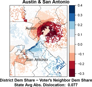
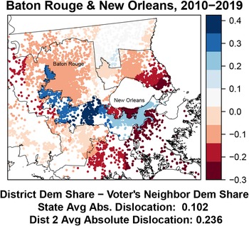
We begin by examining two of the most clear-cut cases of packing and cracking in the United States—the U.S. House of Representatives electoral districts built around Austin, Texas (a clear case of cracking) and the U.S. House of Representatives districts formed out of Baton Rouge and New Orleans in Louisiana (a clear case of packing). These two cases are illustrated in Figures 1 and 2. Voters colored red are those who have been assigned to an electoral district that is substantially more Republican than their nearest neighbors, while voters colored blue are assigned to districts that are substantially more Democratic than their nearest neighbors. Lighter colors indicate voters for whom the difference between the partisanship of the voter’s district and her nearest neighbors is small, while darker colors indicate greater dislocation. Note that the colors are unrelated to the partisanship of the individual voter—they reflect only the difference between the voter’s community and that of her district.
Partisan dislocation in Austin, Texas U.S. House districts. Notes: The above maps plot partisan dislocation scores for a set of representative voters. Dislocation is calculated as the difference in the Democratic vote share of each voter’s assigned district and the Democratic vote share of her k nearest neighbors, where k is the average number of people assigned to each electoral district. District vote shares and the partisanship of nearest neighbors are estimated using precinct-level 2008 U.S. Presidential vote shares as detailed in Section 3. Actual 2014 electoral district boundaries are also included.

Partisan dislocation in New Orleans and Baton Rouge, Louisiana U.S. House districts. Notes: The above maps plot partisan dislocation scores for a set of representative voters. Dislocation is calculated as the difference in the Democratic vote share of each voter’s assigned district and the Democratic vote share of her k nearest neighbors, where k is the average number of people assigned to each electoral district. District vote shares and the partisanship of nearest neighbors are estimated using precinct-level 2008 U.S. Presidential vote shares as detailed in Section 3. Actual 2014 electoral district boundaries are also included.

In Figure 1, it is clear to see how Austin has been effectively cracked into a set of pizza-wedge shaped districts, each of which grabs a portion of the (largely Democratic) residents of Austin and pools them with a rural population of Republicans to create Republican-majority districts. This cracking is evident in the high dislocation scores for residents of Austin, who live in highly Democratic communities but have nevertheless been carved up and placed in Republican districts. The lone exception to this pattern is the long, narrow district that pools a small collection of Austin voters with Democrats in San Antonio to create a packed district, a form of manipulation which is evident in the high dislocation scores of the voters in the middle of this long, narrow district—voters in rural Republican communities who these contorted districts have dislocated in order to make this pooled district.
In Figure 2, we see an illustration of extreme packing in the district that pulls together New Orleans and Baton Rouge. Here we see that voters in both Baton Rouge and New Orleans have been placed in a district that is dramatically more Democratic than their local communities (as shown by regions of bright blue in both cities). At the same time, there is also evidence of cracking in the northern portion of New Orleans which has been carved away from the rest of the city and pooled with (more Republican) voters on the other side of Lake Pontchartrain.
The cases of Baton Rouge and New Orleans also make it clear that while partisan dislocation is a strong indicator of deliberate district manipulation, it cannot speak to whether that manipulation is normatively desirable. In the case of Baton Rouge and New Orleans, for example, part of the rationale for this district is an effort to create a majority-minority district in order to comply with the Voting Rights Act.
With that said, what the partisan dislocation measure can do is evaluate whether majority-minority districts like the Louisiana 2nd district have been drawn in a manner that minimizes overall dislocation. As such, partisan dislocation offers a method for comparing proposals for potential majority-minority districts in a way that makes it possible to police the potential abuse of the majority-minority imperatives for political advantage. After conducting analysis to ascertain the desired racial characteristics of majority-minority districts, it is possible to contrast dislocation scores among a variety of plans with the desired characteristics. This can be done not just for the entire map, but for specific areas in the vicinity of districts designed to facilitate minority representation. Indeed, as we show in Section 5, majority-minority districts can be achieved in Louisiana while also achieving lower levels of voter dislocation than in this enacted plan, which creates a majority-minority district with a black share of the voting-age population that is well beyond anything that could plausibly be required by the Voting Rights Act via extreme district manipulation.
Looking at these figures, one might worry that dislocation is simply a proxy for district compactness. However, this is not the case. Not only are the measures theoretically distinct—one could draw a district with arbitrarily low or high compactness in a state where voters are uniformly distributed, and dislocation would always remain zero—but as discussed in Supplementary Information Section C, they are also quite empirically distinct; more compact districts do tend to have lower levels of dislocation, but the correlation is only
 $\sim 0.275$
.
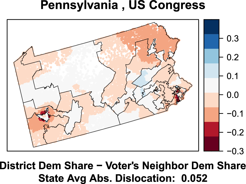
While especially illustrative, these extreme examples are far from unique. Next, let us consider the state of Pennsylvania, a subject of extensive gerrymandering litigation. Figure 3 maps voter partisan dislocation for a representative set of voters. Note that similar patterns can be seen in a number of states that have been accused of gerrymandering in recent years. See Supplementary Information Section B for analogous maps of North Carolina, Texas, Louisiana, and Maryland.
Partisan dislocation in Pennsylvania U.S. House districts. Notes: The above maps plot partisan dislocation scores for a set of representative voters. Dislocation is calculated as the difference in the Democratic vote share of each voter’s assigned district and the Democratic vote share of her k nearest neighbors, where k is the average number of people assigned to each electoral district. Actual 2014 electoral district boundaries are also included.

The Pennsylvania map indicates a high level of dislocation in the inner suburbs around Pittsburgh (in southwest Pennsylvania). Note that voters in the urban core of Pittsburgh experience low levels of dislocation. They are overwhelmingly Democratic, and the legislature drew an extremely Democratic urban Pittsburgh district. However, Democrats in Pittsburgh’s inner ring of suburbs experience high rates of dislocation. These are the kinds of neighborhoods in which Justice Roberts seems to indicate that representational rights may have been abridged. There are large, relatively densely populated areas that are extremely Democratic, but the legislature’s redistricting plan in 2012 embedded them in comfortably majority-Republican districts.
It is easy to see that the Pittsburgh metropolitan area could have been carved up in alternative ways that would have dramatically reduced the striking discontinuity in partisan dislocation on the edges of districts. It would have been possible to divide the city in a way that included more Democrat-leaning suburbs with Democratic urban neighborhoods. This would have led to two rather than one Pittsburgh-oriented districts, but such an arrangement could still involve relatively compact districts.
In Eastern Pennsylvania, the legislature’s gerrymandering efforts involved the creation of meandering districts that aimed not only to pack Democrats into urban Philadelphia, but also to crack Democratic neighborhoods in the educated suburbs, and to prevent smaller Democratic post-industrial cities from stringing together. Again, we see telltale signs of gerrymandering, such as sharp discontinuities in levels of dislocation at district boundaries, such that members of the party drawing the districts (the Republicans) were far less likely to be dislocated than their opponents.
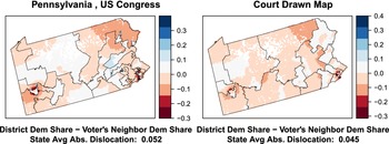
Figure 4 places this map—with districts devised by Republican lawmakers that were later struck down by the Pennsylvania State Supreme Court—beside the map drawn by a Special Master, Stanford Law Professor Nathaniel Persily, at the Court’s request. As the figure shows, the map drawn by the Special Master shows substantially lower levels of partisan dislocation. This illustrates a point we explore more systematically in Section 5: high partisan dislocation scores are not just indicative of individually gerrymandered districts. Because they are an indicator of districts that carve up communities in unnatural ways, states with high dislocation scores tend to be ones in which district manipulation has resulted in one party winning a share of seats that is significantly out of line with their overall vote share, even after controlling for the spatial distribution of voters.
Pennsylvania Republican-drawn and Court-drawn districts. Notes: The above maps plot partisan dislocation scores for a set of representative voters. Dislocation is calculated as the difference in the Democratic vote share of each voter’s assigned district and the Democratic vote share of her k nearest neighbors, where k is the average number of people assigned to each electoral district. Actual 2014 electoral district boundaries are also included.

4.1 District-Level Averages
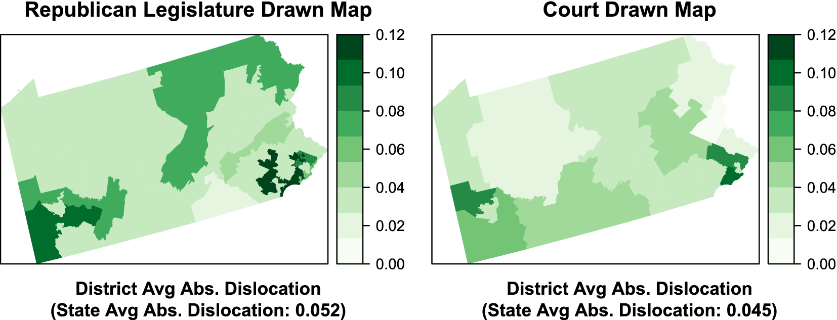
In addition to measuring precinct-level dislocation, we can also aggregate these measures to identify packed and cracked districts. In Figure 5, we color districts by their average absolute partisan dislocation (AAPD)—the average absolute value of representative-voter-level dislocation scores. In particular, the figure again shows the contrast between Pennsylvania’s old maps and those drawn by the Special Master.
Pennsylvania Republican-drawn and Court-drawn districts. Notes: The above maps plot 2014 electoral districts and their AAPD scores. Absolute average dislocation is calculated as the average (over all district voters) of the absolute difference in the Democratic vote share of each voter’s assigned district and the Democratic vote share of her k nearest neighbors, where k is the average number of people assigned to each electoral district. District vote shares and the partisanship of nearest neighbors are estimated using precinct-level 2008 U.S. Presidential vote shares as detailed in Section 3.

The Special Master’s map not only reduces extreme incidences of dislocation around Pittsburgh and in Eastern Pennsylvania, it also reduces overall dislocation. By averaging the absolute magnitude of each voter’s dislocation across the entire state, we can get an overall measure of how much an entire map dislocates voters. In the case of Pennsylvania, for example, we see that the Persily map decreases AAPD by 12.5% (from 0.052 to 0.045).
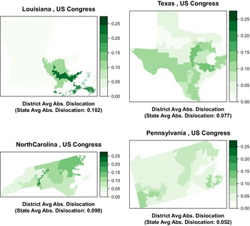
In Figure 6 above, for example, we plot each district’s average absolute dislocation score. Again, we see that dislocation might be a useful guide to the identification of districts where the notion of local representational harm identified by Justice Roberts is most severe.
District average absolute partisan dislocation (AAPD). Notes: The above maps plot 2014 electoral districts and their AAPD scores. Absolute average dislocation is calculated as the average (over all district voters) of the absolute difference in the Democratic vote share of each voter’s assigned district and the Democratic vote share of her k nearest neighbors, where k is the average number of people assigned to each electoral district. District vote shares and the partisanship of nearest neighbors are estimated using precinct-level 2008 U.S. Presidential vote shares as detailed in Section 3.

5 Partisan Dislocation and Global Measures of Unfairness and Gerrymandering
As previously noted, one normative basis for concern about gerrymandering is that it generates global representational inequalities. In this section and the one that follows, we will examine the relationship between Political Dislocation and several measures of representational inequality that are often used as metrics of gerrymandering: unequal weighting of votes for one set of partisan voters versus another, a lack of partisan symmetry in seat shares, unusually large seat shares for one party given its electoral geography, and an unusual lack of electoral responsiveness. First, we focus purely on features of enacted plans, and then we focus on measures that require the generation of a large ensemble of alternative plans.
5.1 Dislocation, Votes, and Seats
Some measures of global representational inequality do not rely on comparisons with a sample of nonpartisan plans, but rather, calculations based on the distribution of votes and seats across districts in a single enacted plan. One approach, meant to capture whether one party’s voters are relatively more “packed” than those of the other, is to simply calculate the difference between the mean and median of the two-party vote share across districts (McDonald and Best Reference McDonald and Best2015). Another approach, called Partisan Symmetry (Katz et al. Reference Katz, King and Rosenblatt2020), is based on the idea that district maps should generate symmetric conversions from vote shares into seat shares, such that when one party has a 60% vote share, the share of seats they win in the legislature is no different from the number of seats the other party would win with a 60% vote share. Note that Partisan Symmetry implies both parties should win 50% of seats if they have 50% vote shares, but does not imply proportionality, since the seat shares won by parties can take on any value when vote shares deviate from 50% so long as they are symmetric.
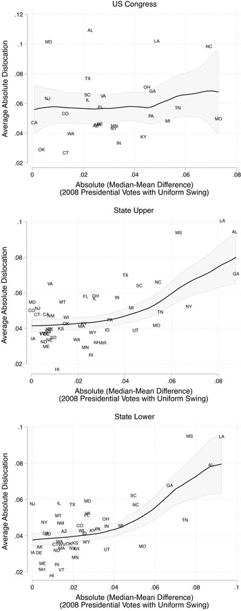
To illustrate the ability of partisan dislocation to detect these notions of gerrymandering, we first plot the relationship between a state’s AAPD and a set of other metrics for measuring gerrymandering. Before presenting these, however, it is important to emphasize that none of these alternative measures are without their own problems (see Katz et al. Reference Katz, King and Rosenblatt2020 for extensive discussion of these issues)—indeed, it is precisely because of their limitations that we have developed our dislocation measure. As such, what we are looking for in these figures is a generally positive relationship, but outliers are to be expected, and as discussed below, often illustrate the value of partisan dislocation.
First, in Figure 7, we plot the AAPD score for each enacted districting plan against what is perhaps the simplest global measures of partisan fairness: the mean–median score. The mean–median score is the the absolute value of the difference between the partisanship of the median district and the cross-district mean, calculated using the same vote data employed in our primary analysis (precinct-level returns from the 2008 presidential election). This measure is thought to be instrumentally valuable in detecting gerrymanders that generate unfair seat allocations by packing voters in homogeneous districts, and is also appealing to those interested in partisan symmetry (McDonald and Best Reference McDonald and Best2015; Best et al. Reference Best, Donahue, Krasno, Magleby and McDonald2018). However, because of its myopic focus on only the median district, mean–median scores can fail to identify gerrymandering manipulations in nonmedian districts, particularly when the statewide partisan baseline is far from 50%. This is related to the issues around responsiveness discussed in Section 5.2, since if the statewide mean is far from 50%, packing and cracking can be employed while maintaining the median district at the mean.Footnote 7 Moreover, unlike our measure, the mean–median score does not take into consideration the political geography of the state or the possible role of the Voting Rights Act.
Absolute average dislocation and absolute median–mean scores. Notes: The above figures plot the average absolute partisan dislocation (AAPD) score for states (averaged across all voters) against each state’s absolute mean–median difference. States with less than 5 districts are omitted. Mean–median differences are calculated as the absolute difference between the Democratic vote share of the median 2014 district and the average Democratic vote share across all districts. District vote shares and the partisan dislocation scores are estimated using precinct-level 2008 U.S. Presidential vote shares as detailed in Section 3. Results are very similar using Democratic vote shares from 2012 to calculate absolute mean–median differences.

As Figure 7 shows, while the correlation is not overwhelming, AAPD does tend to track with mean–median scores in the enacted plans.Footnote 8 But it is from the exceptions that perhaps we learn the most. For example, consider Texas’ U.S. Congressional districts. As discussed above, the Texas legislature has clearly engaged in gerrymandering, and yet scores low on the mean–median measure. In terms of AAPD, by contrast, Texas scores as the sixth most gerrymandered state in the Union. Similarly Maryland, subject of the recent U.S. Supreme Court gerrymandering case Benisek v. Lamone, has a low mean–median score, but the third-highest AAPD score. Missouri demonstrates a high mean–median difference, in part because of the concentration of Democrats in St. Louis and Kansas City and the explicit goal of producing a Congressional district that can be won by minority candidates in both cities. Yet the relatively moderate dislocation value indicates that it was possible to achieve this goal without exceptional levels of dislocation.
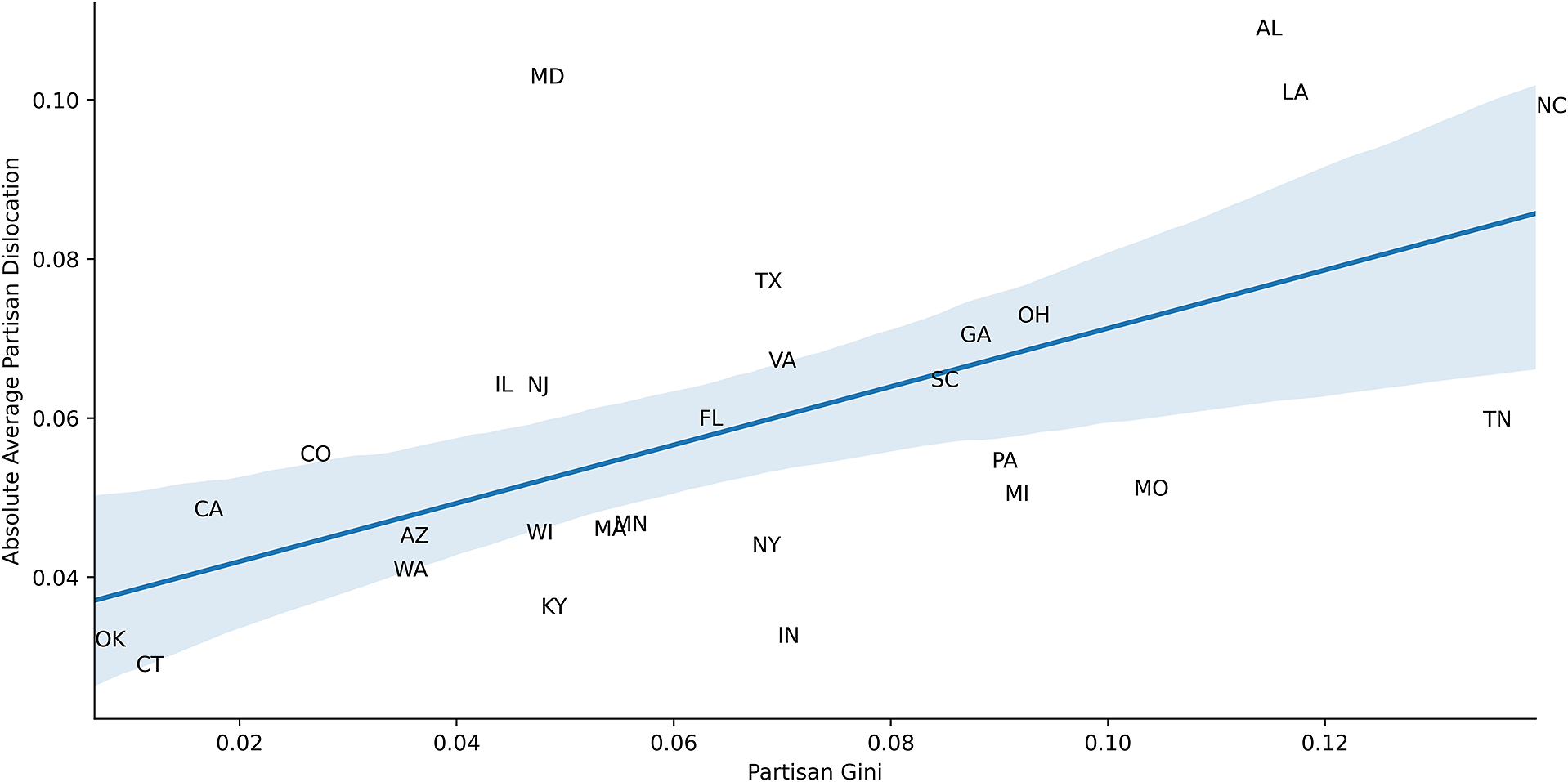
In Figure 8, for Congressional districts, we plot AAPD against the Partisan Gini, a measure of the asymmetry of the vote-seat curve (i.e. the degree to which Partisan Symmetry has been violated). This function was introduced as measure 7 in (Grofman Reference Grofman1983) and more recently in (Katz et al. Reference Katz, King and Rosenblatt2020). An electoral system is said to satisfy the partisan symmetry standard if this value is zero. As the Figure shows, we find a very strong positive relationship between AAPD and the Partisan Gini. That is to say, the enacted plans that produce high levels of partisan dislocation are also those that produce high levels of partisan asymmetry, such that one party (typically the Republican Party) can expect a relatively high seat share given its vote share.
Partisan Gini and average absolute partisan dislocation (AAPD). Notes: The above figure plots AAPD scores for states’ enacted 2014 U.S. Congressional district plans against Partisan Gini scores for those same districts. States with less than 5 districts are omitted. All voting data come from the 2008 Presidential Election. Shaded regions represent 95% confidence intervals.

Finally, as shown in Table 1 above, there is also substantial circumstantial evidence that AAPD scores capture deliberate map manipulation, as AAPD tends to be highest in states where district maps were drawn under unified party control.Footnote 9 This is especially true when districts were drawn under unified Republican control, reflecting the success of Republican lawmakers in their efforts to maximize the opportunities presented by redistricting in the early 2010s.
State average absolute dislocation by district creators.

5.2 Dislocation and Simulated Districts
The problem with simple statistics generated from the distribution of votes and seats across districts associated with enacted plans, of course, is that they do not take the political geography of the state into account. Nor do they take into account the possibility that unfairness or partisan asymmetry may have been driven, in whole or in part, by efforts to comply with the Voting Rights Act. The solution in the academic literature, and in court, is to compare properties of enacted district maps with ensembles of thousands of sampled maps.
Plaintiffs have argued that voters’ rights to equal representation have been violated when gerrymandering results in a party receiving fewer seats than they would absent manipulation of district boundaries for political gain. In this framework, parties are not entitled to proportional representation, but through simulation-based methods, plaintiffs attempt to argue that enacted maps result in seat shares that do not arise naturally given the vote shares and the spatial distribution of voters in a state. An additional approach is to contrast the responsiveness of the enacted and simulated maps.
In this section, we augment our analysis by generating 100,000 alternative maps for each state. This allows us to do two useful things. First, we can examine the relationship between our measure of gerrymandering and ensemble-based measures that are increasingly used in court cases. Second, we demonstrate that our measure provides an attractive alternative to anticipated seat shares as a basis for contrasting enacted and sampled plans.
To generate a large collection of comparison plans, we use the ReCom Markov chain introduced in DeFord et al. Reference DeFord, Duchin and Solomon2021 as implemented in the GerryChain software package (MGGG 2019)Footnote 10 to construct ensembles of 100,000 random district plans for each state. The plans generated by the Markov chain are contiguous, population balanced to within 1% of ideal, and are further constrained to preserve the existence of majority-minority districts (to ensure compliance with the Voting Rights Act). Additional details can be found in Supplementary Information Section D. Note that when calculating seat shares, we add a uniform swing of 3.69% to the two-party vote share of Republicans to bring the overall vote share of Democrats and Republicans to 50–50 nationally. All other measures are uniform-swing invariant.
Using these comparison plans, we can now compare AAPD scores to simulation-based metrics of gerrymandering. First, a standard approach is to aggregate precinct-level partisan data to the level of enacted and simulated districts, and examine the difference between the anticipated seat shares for the two parties associated with the enacted plan and those of the simulated plans. Another approach is to examine the difference between the partisan symmetry of the enacted plan and those of the ensemble of simulated plans. A third and more recent approach is to examine the responsiveness of enacted and simulated plans. We measure responsiveness using the Gerrymandering Index, based on the work of Herschlag et al. analyzing ensembles of plans in North Carolina and Wisconsin (Herschlag, Ravier, and Mattingly Reference Herschlag, Ravier and Mattingly2017; Herschlag et al. Reference Herschlag, Kang, Luo, Graves, Bangia, Ravier and Mattingly2020). The index is designed to detect maps that create an unusual number of “safe districts” (with, say, a 55% or 60% vote share), and takes on large values when those are present.Footnote 11
These clumps of safe districts are often used by gerrymanderers to ensure that seat shares will not respond smoothly to changes in overall vote shares (i.e., seat shares will not be responsive to changes in vote shares)—instead, because so many districts are stacked with 5–10 percentage point margins, vote swings of less than 5%–10% will have no impact on the outcome of elections in those districts, preventing seat shares from responding to changes in vote shares. Note that this metric can only be calculated with the use of simulated ensembles.
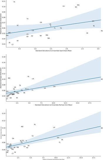
Figure 9 below plots AAPD against the distance (in standard deviations) between ensemble average values of various map attributes and those of enacted plans. In particular, the figure compares ensemble and enacted plans in terms of Democratic seat shares, Political Gini, and finally, the Gerrymandering Index described above.
Notes: The above figures plot average absolute partisan dislocation (AAPD) scores for states’ enacted 2014 U.S. Congressional district plans against simulation-based measures of gerrymandering. Simulation-based measures report the difference between enacted plan scores and the average score across all ensemble plans (in standard deviations of simulated district plans). Figures include only results for states with five or more districts. As detailed in Supplementary Information Section D, simulated district plans are subject to compactness and population balance constraints, and all plans have the same number of districts that are more than 45% minority (Black or Hispanic) as enacted plans. Shaded regions represent 95% confidence intervals.

We see a clear positive correlation between our measure of gerrymandering and the simulation-based measure. Note that this relationship is clearly in evidence despite the fact that AAPD scores are not normalized against simulation averages—these are raw scores. As shown in Supplementary Information Section E, correlations are even stronger when we also normalize AAPD scores (by reporting the difference between AAPD for the enacted plan and the average AAPD among simulated districts), but we report the raw scores here to illustrate the value of our measure even absent simulations.
The results also illustrate the limitations of other measures. Seats-based and symmetry-based approaches, for example, tend not to identify Texas as being particularly gerrymandered, while AAPD flags it as a significant gerrymander. Only in the Gerrymandering Index results do we see a simulation-based measure that characterizes Texas as a notable gerrymander: it is the seventh most gerrymandered state in terms of the responsiveness dimension, while it is the fifth most according to AAPD.
In sum, we view these scatterplots as a validation of our approach. It reaches broadly similar conclusions as existing simulation-based approaches, without requiring a complex computational endeavor that can take considerable time, computing power, and technical expertise. Moreover, areas of disagreement between our approach and existing approaches suggest that our approach can pick up a different class of gerrymanders that might be missed by other approaches.
However, partisan dislocation might be most useful not as a substitute, but as a complement to redistricting simulations. As discussed above, it is not always clear which underlying election results should be used in the calculation of hypothetical seat shares, partisan symmetry, or responsiveness. In some situations, the choice can be consequential. Even in an era of nationalized politics, the spatial distribution of voting behavior can vary substantially from one race to another, even for races held on the same day (Rodden and Weighill Reference Rodden, Weighill and Duchin2020).
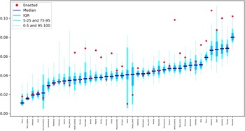
AAPD can also be a useful alternative metric for comparing ensembles of simulated maps with enacted maps. Figure 10 below plots, for each state, the distribution of AAPD score for 100,000 simulated district plans as well as the score for the currently enacted plan. As the figure clearly shows, it is not just the case that the existing maps of known gerrymanders have high AAPD scores compared to other states, as demonstrated above. They also have much higher AAPD scores than randomly generated districting plans for their own state. Analyses like that contained in Figure 10 might prove to be a very useful diagnostic tool. The outliers in Figure 10 seems to identify all of the well-known gerrymanders of the last redistricting cycle without producing any worrisome false positives.
AAPD might be especially useful in contexts like Louisiana, where states are required to establish majority-minority districts. As noted in Section 4, because partisan dislocation scores tend to identify “unnatural” districting plans, there may be occasions where higher-than-usual dislocation scores are necessary in order to achieve other goals, like facilitating the ability of minorities to elect candidates of choice, if these goals require drawing “unnatural” districts. In states like Alabama, or in Northern Florida, one might need to tolerate a relatively high level of dislocation in order to draw a district where minorities can elect candidates of choice. But partisan dislocation also helps measure the degree to which communities of like-minded voters have been torn asunder to achieve these ends. Indeed, as we can see in Figure 10, the vast majority of simulated district plans have far lower partisan dislocation scores than Louisiana’s enacted plan. The same is true of Alabama, Florida, North Carolina, and Virginia. Recall that in each case, the simulated plans are explicitly drawn so as to provide similar numbers of districts in which minorities can elect candidates of choice as the enacted plans. In short, partisan dislocation provides a way to identify manipulation above and beyond that which was required in order to comply with the VRA, and to provide detailed maps of precisely where the manipulation took place.
6 Partisan Fairness versus Dislocation
If one accepts the claim that representation of the interests of like-minded neighbors is a crucial purpose of geographic districts (Curiel and Steelman Reference Curiel and Steelman2018), and accepts that partisan dislocation undermines this type of representation, one might be tempted to conclude that map-drawers should simply endeavor to minimize dislocation. However, before accepting this claim, one must have a clear sense of whether plans that exhibit low levels of dislocation might have other countervailing normative disadvantages. Above all, a single-minded effort to minimize partisan dislocation might inadvertently undermine the goal of partisan symmetry.
Maps with low dislocation scores might accurately reflect voter geography, but they may also serve to entrench the partisan asymmetry that emerges from the clustering of Democratic voters in cities (Rodden Reference Rodden2019). One way to view this residential clustering of Democrats is as a choice made by voters—and thus not a situation requiring accommodation by map makers. But others might argue that low-income voters living in segregated communities reinforced by decades of redlining and racially biased housing policies cannot really be said to have “chosen” to live in communities that tend to result in less efficient representation. In many societies, low-income renters are often spatially concentrated due to the nature of urban form. In any case, for those who wish to elevate partisan fairness as the primary goal in redistricting, it may sometimes be necessary to break up urban concentrations of Democrats, thus creating plans with high levels of dislocation.
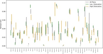
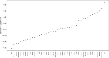
Our redistricting simulations provide us with an ideal opportunity to explore this potential tension between “naturalness” and other normative goals, like partisan symmetry. In Figures 11 and 12, we examine the relationship between partisan dislocation scores and the partisan Gini. In Figure 11, we split our random plan ensembles into the 1% with the highest AAPD, the 1% with the lowest AAPD. We then plot the inter-quartile range of high AAPD plans, low AAPD plans, and the full ensemble of plans in terms of their Partisan Gini scores. Figure 12 presents the correlation between AAPD and the Partisan Gini in each state’s ensemble.
Average absolute partisan dislocation (AAPD) scores for enacted and random districts. Notes: The above figure plots AAPD scores for both enacted district plans and the distribution of AAPD scores in simulated district plans. As detailed in Supplementary Information Section D, simulated district plans are subject to population balance constraints and use a proposal that produces compact plans, and all plans have the same number of districts that are more than 45% minority (Black or Hispanic) as enacted plans.

Distribution of partisan GINI among plans in redistricting ensemble, by level of partisan dislocation. Notes: The above figure plots the inter-quartile range of the 1% of plans with the highest AAPD, the 1% of plans with the lowest AAPD, and that of all plans in the ensemble in terms of the Partisan Gini score.

Correlations Between Partisan Dislocation and Partisan Asymmetry Within Each State’s Redistricting Ensemble. Notes: Drawing on the ensemble of redistricting plans for each state, the above figure plots the Pearson correlation coefficient between the Partisan GINI and AAPD. A positive coefficient indicates that within the redistricting ensemble for that state, higher levels of dislocation are correlated with higher partisan GINI (more partisan asymmetry).

Figure 11 displays interesting heterogeneity across states when it comes to partisan symmetry. In states where Democrats are not highly concentrated in space at the scale of Congressional districts, like Iowa with its dispersed small cities, or Arizona with its vast suburban sprawl, we see that the plans with low and high levels of dislocation are not all that different from the overall distribution in terms of partisan symmetry, and if anything, higher levels of dislocation are associated with higher levels of partisan asymmetry. In these states, the goal of minimizing dislocation and that of partisan fairness may not be in conflict.
However, the story changes when we look at the early-industrializing states, as well as some Southern states, where Democrats are concentrated in large cities. Examples of the former include Illinois, Michigan, Missouri, Minnesota, Pennsylvania, and Wisconsin. The latter include Georgia, Tennessee, Kentucky, and Texas. In these states, the plans with the highest levels of Dislocation are actually those with the lowest partisan Gini. That is to say, they are the plans that minimize the partisan asymmetry associated with the geographic clustering of Democrats. Likewise, the plans with the lowest levels of dislocation—those that keep local communities of co-partisans together—are the ones that generate the highest levels of partisan asymmetry in the transformation of votes to seats.
This indicates that in a number of populous states, the goals of minimizing partisan dislocation and enhancing partisan fairness might be in direct conflict. In order to facilitate partisan symmetry in a state like Illinois—where Democrats are highly concentrated in Chicago—it is necessary to break up communities of co-partisans. In redistricting, unfortunately, it is not always the case that all good things go together.
7 Conclusion
Partisan gerrymandering is difficult to measure, and it is conceptually distinct from partisan fairness, which is typically measured globally rather than locally. Federal courts have determined that they are unwilling to enter the thicket of partisan fairness. It is evident that courts would benefit from a measure that focuses clearly on intentional packing and cracking of local communities, rather than fairness, and does so at the level of specific districts or even neighborhoods. We have developed such a measure, called partisan dislocation, and we have shown that it is well-suited to the identification of voters that have been cracked or packed. At the level of states, an aggregated measure of dislocation is weakly correlated with global measures of fairness, and more strongly correlated with existing measures of gerrymandering that rely on comparisons of simulated and enacted plans.
Partisan dislocation might be useful for future litigants wishing to establish that plaintiffs have been directly harmed by being placed in packed or cracked districts. Partisan dislocation comports with intuitions about how gerrymandering is accomplished and identifies deliberate district manipulations. It can be used to demonstrate the representational harm experienced by residents of specific neighborhoods, and thus can be used to help plaintiffs establish standing to sue. Moreover, it allows for rigorous district-specific gerrymandering analysis. Following the logic of racial gerrymandering cases, state courts might be willing to strike down specific offending districts without throwing out the entire map, and our measure provides them with the means to do so.
When aggregated to the state level, partisan dislocation also holds out promise as a statewide measure of gerrymandering that fills in some of the blind spots of existing global approaches. However, we have also shown that different states have different baseline levels of dislocation. As a result, in high-stakes situations like gerrymandering litigation, partisan dislocation is probably best analyzed in explicit comparison with simulated ensembles that take political geography and minority representation into account. A gerrymandered plan will exhibit significantly higher levels of dislocation than a sample of non-partisan plans.
However, as Bernard Grofman points out, if one accepts the logic of the Supreme Court of the United States in Gill v. Whitford and Rucho et al v. Common Cause et al., a “statewide standard for partisan gerrymandering is almost certainly doomed to failure” (Grofman Reference Grofman2019), p. 95. For that reason, the most fruitful application of partisan dislocation is not as a blunt aggregate measure, but rather, as a fine-grained local measure.
Outside of the courts, partisan dislocation might prove to be a useful metric for legislators, commissioners, or members of the public when drawing and evaluating their own maps. We have demonstrated, however, that in some settings, there may be inevitable trade-offs between the goal of achieving partisan fairness and that of keeping geographic clusters of like-minded people together. Even if one’s primary goal is partisan fairness or an acceptable level of representation for minority groups, partisan dislocation may still be valuable as a tool for ensuring that states enact the least disruptive implementation that achieves a given goal. This can be accomplished by looking for plans that minimize partisan dislocation subject to other fairness or racial representation constraints. For example, the creation of majority-minority districts has increasingly become a convenient excuse for gerrymandering in many states. As shown in Louisiana, however, partisan dislocation can be used to compare different plans that achieve the same goal, and identify those that seem to achieve that goal in more or less manipulative ways. In doing so, partisan dislocation may help limit the space for manipulation in the name of other objectives. When choosing between plans that exhibit similar levels of partisan symmetry, commissioners might look for plans with lower levels of partisan dislocation.
A worthy goal for future research is to generate additional measures, inspired by the dislocation concept, that are less geared toward ex-post gerrymandering detection, and better suited for prospective district-drawers who wish to thread the needle between fairness and “naturalness.” For instance, instead of calculating the continuous difference between the vote share of each representative voter’s neighborhood and that of the enacted district, one could try to maximize the share of voters with a match between the binary partisanship of their neighborhood (is it majority Democratic or Republican?) and that of the enacted district.
Finally, our measure might also be useful in empirical political research in economics and political science. Models of distributive politics point to important implications for the distribution of resources when legislative district lines carve up political communities (Stashko Reference Stashko2020). For instance, a strategic politician might face incentives to ignore clusters of dislocated members of the minority out-party within a district, or to place unpopular projects, like low-income housing developments or waste processing facilities, in such neighborhoods. If such phenomena are sufficiently pronounced, it is plausible that redistricting would have an impact on property values in dislocated communities. Moreover, a literature on representation (e.g., Niemi et al. Reference Niemi, Powell and Bicknell1986; Curiel and Steelman Reference Curiel and Steelman2018) argues that breaking up local communities of like-minded voters has implications for turnout, citizen engagement and knowledge, and the strength of connections between representatives and their voters. Partisan dislocation is well-suited for future studies in this tradition.
Data Availability Statement
Replication code for this article has been published in Code Ocean and can be viewed interactively at https://doi.org/10.24433/CO.7980425.v1 (DeFord, Eubank, and Rodden Reference DeFord, Eubank and Rodden2020a). A preservation copy of the same code and data can also be accessed via Dataverse at https://doi.org/10.7910/DVN/MERAIC (DeFord, Eubank, and Rodden Reference DeFord, Eubank and Rodden2020b).
Supplementary Material
For supplementary material accompanying this paper, please visit https://doi.org/10.1017/pan.2021.13