1 Introduction
Turbulence at and very near the free surface has a controlling influence on air–water gas fluxes, the understanding of which is important for many environmental and geophysical problems, such as the uptake of CO
 $_{2}$
in the oceans. Gas transport through liquid interfaces is usually parametrized in terms of turbulent properties of the fluid at or very close to the free surface, such as the turbulent kinetic energy (
 $q$
), the turbulent energy dissipation (
 $\unicode[STIX]{x1D700}$
) or the root-mean-square (r.m.s.) of the velocity divergence at the surface (Jähne & Haussecker Reference Jähne and Haussecker1998; Turney & Banerjee Reference Turney and Banerjee2013; Variano & Cowen Reference Variano and Cowen2013). These quantities are usually estimated from values below the surface, because performing experimental measurements at or very close to the surface is very challenging due to the surface dynamics and the small thickness of the region of interest.
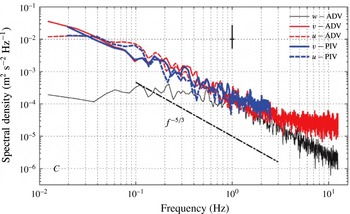
Chickadel et al. (Reference Chickadel, Talke, Horner-Devine and Jessup2011) were among the first to overcome those difficulties. In an experimental campaign at the Snohomish River WA, they measured the horizontal velocities at the free surface using thermal infrared-based particle image velocimetry (IR PIV). Velocity frequency spectra taken from their paper are shown in figure 1. The figure shows spectra of the lateral
 $u$
and along-stream
 $v$
velocity components measured by IR PIV, together with all three components measured by acoustic Doppler velocimetry (ADV) at 0.02 m below the river surface. The experiments were performed at night under calm and clear atmospheric conditions, with an essentially flat free surface on the river (more details of the experiment are reported in Chickadel et al. (Reference Chickadel, Talke, Horner-Devine and Jessup2011) and Talke et al. (Reference Talke, Horner-Devine, Chickadel and Jessup2013)).
Spectra from the measured
 $u$
,
 $v$
and
 $w$
(vertical) components of the velocity using ADV (0.02 m depth) and IR PIV at the Snohomish River, WA. The dash-dotted line corresponds to
 $f^{-5/3}$
. Copyright 2011 IEEE. Reprinted, with permission, from Chickadel et al. (Reference Chickadel, Talke, Horner-Devine and Jessup2011).

Chickadel et al. (Reference Chickadel, Talke, Horner-Devine and Jessup2011) showed for the first time that near-surface turbulence properties in a river can be determined remotely. For frequencies less than approximately 1 Hz, the agreement between the
 $u$
and
 $v$
spectra obtained from IR PIV and ADV in figure 1 is remarkable. Also, direct measurements of the turbulent kinetic energy, and inferred kinetic energy dissipation rate, obtained using the image-based IR PIV method were within 8 % of the in situ ADV measurements over a six hour time period and with more than an order of magnitude variation in the measured parameters. These results suggest that the IR PIV method holds significant promise for remote sensing of turbulence in a wide range of geophysical flows and may be used in the future, for example, to drive inverse models or to understand turbulent gas fluxes at the air–water surface (see, e.g. Moog & Jirka Reference Moog and Jirka1999). Since the IR PIV method is based on the image content from the thermal IR whose penetration depth is less than 1 mm below the surface, these are true surface measurements.
The value of this novel measurement approach requires an understanding of two fundamental turbulence questions. First, why do the horizontal velocity spectra shown in figure 1 exhibit a
 $-5/3$
slope when the turbulence there is highly anisotropic and it is strongly affected by the free surface? And second, can the relationship between the turbulence parameters at the surface and below the surface be generalized, such that the subsurface turbulence information can be inferred from the IR PIV, and vice versa? The objective of the present study is to gain some insight into these questions.
One of the issues of interest here is then the fact that the spectra of the horizontal components of the velocity follow a
 $f^{-5/3}$
law very closely below about 1 Hz, which corresponds to horizontal wavelengths above 0.8 m (using the Taylor hypothesis and the current speed, approximately
 $0.8~\text{m}~\text{s}^{-1}$
) at distances to the free surface smaller than 0.02 m. Note that this cannot be a Kolmogorov inertial range, since neither isotropy nor vertical homogeneity are satisfied for that wavelength range. First, the horizontal velocities are much larger than vertical velocities (compare
 $u$
and
 $v$
to
 $w$
in figure 1). Second, at the location of the ADV measurements, only vertical wavelengths below 0.02 m can be assumed to be homogeneous. Longer wavelengths in the vertical direction are inhomogeneous, since they see the free surface. By the same logic, all wavelengths at the free surface (IR PIV measurements) are vertically inhomogeneous.
The prevailing theory to explain the near-surface dynamics is the theoretical framework put forward by Hunt & Graham (Reference Hunt and Graham1978) and related works (to be discussed in the next section). This theoretical framework describes the changes in variances and spectra in the region influenced by the surface in terms of the properties of the turbulence far from the surface. The theory suggests that as a weak turbulent eddy approaches the surface, energy is first transformed from vertical to horizontal velocities without dissipation (in the source or blockage layer), and then dissipated in a thin layer very close to the surface (in the viscous layer). It is interesting to note that, within this framework, the
 $-5/3$
law in figure 1 is a consequence of the spectral distribution of energy far below the surface.
In the present paper, we put forward an alternative hypothesis, which is that the
 $-5/3$
behaviour observed in figure 1 is an intrinsic property of turbulent fluctuations very close to a free surface. The motivation for this alternative view is the similarity between the spectra shown in figure 1 and the results obtained from numerical simulations (e.g. Riley & de Bruyn Kops Reference Riley and de Bruyn Kops2003; Lindborg Reference Lindborg2006; and Brethouwer et al.
Reference Brethouwer, Billant, Lindborg and Chomaz2007), field data (e.g. Riley & Lindborg Reference Riley and Lindborg2008) and similarity hypotheses (Lindborg Reference Lindborg2006) for strongly stably stratified turbulent flows (of course a free surface itself is strongly stably stratified). In such flows, at large horizontal scales the vertical component of the kinetic energy is suppressed by the density stratification, while the horizontal spectra of the horizontal velocities exhibit a
 $-$
5/3 behaviour. Such flows are now termed ‘stratified turbulence’.
Riley & Lindborg (Reference Riley, Lindborg, Davidson, Kaneda and Sreenivasan2013) provide a detailed theoretical explanation of the
 $-5/3$
behaviour in stratified turbulence, which is briefly reproduced here for completeness. Consider a turbulent flow in a stable density-stratified fluid with uniform ambient density gradient
 $\text{d}\bar{\unicode[STIX]{x1D70C}}/\text{d}z<0$
, and hence uniform buoyancy frequency
 $N=\sqrt{-g/\unicode[STIX]{x1D70C}_{0}\cdot \text{d}\bar{\unicode[STIX]{x1D70C}}/\text{d}z}$
, where
 $\bar{\unicode[STIX]{x1D70C}}(z)$
is the ambient density field,
 $z$
is the vertical coordinate,
 $g$
the gravitational acceleration and
 $\unicode[STIX]{x1D70C}_{0}$
a reference density. Assume that the characteristic horizontal velocity
 $U$
and horizontal length scale
 $\ell _{h}$
satisfy the following:
-
(i) the Reynolds number
 $R_{h}=U\ell _{h}/\unicode[STIX]{x1D708}$
is very large, where
$\unicode[STIX]{x1D708}$
is the kinematic viscosity;
-
(ii) the Froude number
$F_{h}=U/N\ell _{h}$
is small, implying the effects of stable stratification are in some sense dominant; and -
(iii) the buoyancy Reynolds number
${\mathcal{R}}=\unicode[STIX]{x1D700}/\unicode[STIX]{x1D708}N^{2}$
is very large, where
$\unicode[STIX]{x1D700}$
is the turbulent dissipation rate.


With these assumptions,
 $\ell _{h}$
is much larger than the Ozmidov length scale
 $\ell _{O}=(\unicode[STIX]{x1D700}/N^{3})^{1/2}=F_{h}^{3/2}\ell _{h}$
, which is in turn much larger than the Kolmogorov length scale
 $\unicode[STIX]{x1D702}=(\unicode[STIX]{x1D708}^{3}/\unicode[STIX]{x1D700})^{1/4}$
. For length scales in the range
 $[\unicode[STIX]{x1D702},\ell _{O}]$
, turbulence is more or less isotropic. However, for horizontal length scales in the range
 $[\ell _{O},\ell _{h}]$
, stable stratification suppress the vertical motions, resulting in a vertical component of the velocity much smaller than either of the horizontal components (Lindborg Reference Lindborg2006). Then, dimensional analysis arguments dictate that the energy spectrum of the horizontal velocities for horizontal length scales between
 $\ell _{O}$
and
 $\ell _{h}$
(corresponding to horizontal wavenumbers
 $k_{h}$
such that
 $1/\ell _{h}\ll k_{h}\ll 1/\ell _{O}$
) can only depend on the horizontal wavenumber
 $k_{h}$
and the energy transfer
 $\unicode[STIX]{x1D700}$
(if the energy cascade is in equilibrium), resulting in
 $E_{h}(k_{h})\sim \unicode[STIX]{x1D700}^{2/3}k_{h}^{-5/3}$
. These horizontal scales also tend to develop strong vertical shearing (Lilly Reference Lilly1983; Billant & Chomaz Reference Billant and Chomaz2001; Riley & de Bruyn Kops Reference Riley and de Bruyn Kops2003), which triggers the transition to homogeneous isotropic turbulence for scales smaller than
 $\ell _{O}$
.
In the present article, we hypothesize that the dynamics of the turbulent flow near the free surface is very similar to that of strongly stratified turbulence. In particular, at large horizontal scales and close to the free surface, the vertical velocity is suppressed while the vertical shearing of the horizontal flow is left uninhibited. Consider
 $L$
as the horizontal scale of the energy-containing motions,
 $\unicode[STIX]{x1D6FF}$
the distance from the free surface, and
 $\unicode[STIX]{x0394}U$
the characteristic velocity resulting from the vertical shearing, equal to the velocity difference at a distance
 $\unicode[STIX]{x1D6FF}$
from the free surface. Then, if
 $Re_{\unicode[STIX]{x1D6FF}}=\unicode[STIX]{x0394}U\unicode[STIX]{x1D6FF}/\unicode[STIX]{x1D708}$
is large enough, shear instabilities would be expected to develop, enhancing turbulent motions on the scale
 $\unicode[STIX]{x1D6FF}$
and below, where a more isotropic turbulence would be expected. If the ratio
 $L/\unicode[STIX]{x1D6FF}$
is large enough, then, in analogy with stratified turbulence, the horizontal spectra of horizontal velocity of the form
 $\unicode[STIX]{x1D6FC}\unicode[STIX]{x1D700}^{2/3}k_{h}^{-5/3}$
would be expected for intermediate wavelengths (Lindborg Reference Lindborg2006). While in stratified turbulence the
 $-5/3$
range appears between
 $\ell _{h}$
and
 $\ell _{O}$
, in the free surface turbulence it would be expected to appear between
 $L$
and
 $\unicode[STIX]{x1D6FF}$
, where
 $\ell _{O}$
and
 $\unicode[STIX]{x1D6FF}$
play the same dynamical role (i.e. the wavelength at which isotropy is recovered). In the field data,
 $\unicode[STIX]{x1D6FF}=2~\text{cm}$
, whereas the characteristic length scale of the horizontal velocities can be conservatively estimated to be
 $L=8~\text{m}$
, taking
 $f=0.1~\text{Hz}$
and the current speed of
 $0.8~\text{m}~\text{s}^{-1}$
. Clearly then
 $L/\unicode[STIX]{x1D6FF}=400$
is large and such an inertial-type range might be expected to exist.
To test this hypothesis, and to help understand the near-surface dynamics observed in the field measurements, we performed a direct numerical simulation (DNS) of turbulence near a free surface. We modelled the free surface with a stress-free boundary condition on a flat surface, which should also be a good approximation to the free surface of the river in the experiments of Chickadel et al. (Reference Chickadel, Talke, Horner-Devine and Jessup2011). In the next section we discuss some past research on turbulent flow near a stress-free surface. Then, we describe the numerical method, initial conditions and main parameters of the cases computed. In § 4 we discuss the results of the simulations, and in the final section we summarize our conclusions, suggest further research to be done and discuss other implications of the work.
2 Background
Perhaps the first effort to set up a theoretical framework for understanding turbulence near a relatively flat, stress-free surface is the paper by Hunt & Graham (Reference Hunt and Graham1978), who added an irrotational part to homogeneous turbulence to satisfy a no-slip boundary condition at a surface. Then, using rapid distortion theory (which implies the linearization of the equations), they were able to predict the behaviour of the components of turbulent kinetic energy with distance away from the boundary. They also identified a blockage layer, the region adjacent to the surface where the velocity fluctuations normal to the surface go from the interior flow value to zero at the surface, and a viscous layer, the region across which the shear stress goes from zero at the boundary to a peak value near the boundary. Their work was extended first by Hunt (Reference Hunt1984) to include some nonlinear features, and later by Teixeira & Belcher (Reference Teixeira and Belcher2000) to add viscous effects.
Brumley & Jirka (Reference Brumley and Jirka1987) studied turbulence in a square water tank with a free surface, by vertically oscillating a horizontal grid at depth in the tank. Adequate agreement with the Hunt/Graham model was obtained; in addition they found that the blockage layer (or surface influenced layer) is about one integral scale in depth, where the integral scale is based upon the interior flow. Later Perot & Moin (Reference Perot and Moin1995) used DNS to study the interaction of turbulence with shear-free solid boundaries, impermeable boundaries, and stress-free boundaries. For the stress-free case they identified two types of flow structures near the boundaries, splats and antisplats, linked to the intercomponent energy transfer (pressure–strain). The splats (antisplats) are regions where the vertical velocity points towards (away) the boundary, increasing (decreasing) the local pressure and producing a positive (negative) horizontal divergence. Hence, in splats energy is transferred from the vertical to the horizontal components, while the energy is transferred back from horizontal to vertical motions in the antisplats. Perot & Moin (Reference Perot and Moin1995) concluded that the Hunt/Graham analysis did not apply to the evolution of turbulence near boundary surfaces, although they noted that there was significant evidence which supported the model. The numerical results of Perot & Moin (Reference Perot and Moin1995) were confirmed experimentally by Aronson, Johansson & Löfdahl (Reference Aronson, Johansson and Löfdahl1997), in particular the profiles of the pressure–strain terms. They concluded that the Hunt/Graham theory only holds for the initial transient, an observation also confirmed by others. Later, Calmet & Magnaudet (Reference Calmet and Magnaudet2003) performed large-eddy simulations (LES) of open-channel flow using a dynamic subgrid-scale model, focusing in particular on the near-surface region. They found good agreement with the Hunt/Graham model outside the viscous layer, and their results suggested that the good agreement is not restricted to short times. Magnaudet (Reference Magnaudet2003) performed theoretical analysis and reconciled most existing results, finding the Hunt/Graham model to be a leading-order approximation capable of describing both the short- and long-time evolution of the shear-free boundary layers. More recently, Campagne et al. (Reference Campagne, Cazalbou, Joly and Chassaing2009) used DNS to study turbulence near a stress-free boundary and developed scalings for the size of the local layers depending on local turbulence parameters.
Besides the abundant literature revolving around the Hunt/Graham theory, we have only been able to find a few papers showing velocity spectra measured very near the free surface, which might be consistent with the field measurements in figure 1. Brumley & Jirka (Reference Brumley and Jirka1987) show that the horizontal spectra of the vertical velocity is suppressed at low wavenumbers near the free surface. Furthermore, closer to the surface (at distances equal to 4 % and 0.16 % of the integral scale) the horizontal spectra of the horizontal velocity appears to show an inertial range at horizontal scales well above the isotropic range. Such an inertial range is difficult to determine confidently, however, due to the scatter in the data. In a later study, Herlina & Jirka (Reference Jirka2008) used an experimental set-up similar to that of Brumley & Jirka (Reference Brumley and Jirka1987), using PIV to measure velocity. At 0.17 mm from the free surface, and over the range of frequencies presented, the energy spectrum of the vertical velocity was extremely low. The spectrum of the horizontal velocity, however, exhibited a
 $-5/3$
range, consistent with the field observations presented in figure 1. The authors realized that the result was not due to a three-dimensional turbulence inertial range, since the flow in the vertical direction is restricted, and pointed out that the flow becomes more two-dimensional. No additional explanation, however, was offered for the behaviour of the spectral properties of the flow. Note that our hypothesis for the spectral behaviour of the flow discussed in the previous section relies on the non-two-dimensionality of the flow, specifically the vertical variation of the horizontal velocities.
3 Methodology
In order to analyse the behaviour of a turbulent flow in the vicinity of a free surface, we perform a DNS of incompressible, decaying turbulence bounded by a no-slip wall (bottom,
 $z=0$
) and a stress-free surface (top,
 $z=2\unicode[STIX]{x03C0}L_{0}$
, where
 $L_{0}$
is the wavelength at which the initial velocity spectrum peaks, see the next paragraph). The flow is assumed to be homogeneous in the horizontal directions (
 $x$
and
 $y$
), which are modelled as being periodic with periodicity
 $L_{x}=L_{y}=8\unicode[STIX]{x03C0}L_{0}$
. Note that the computational domain is four times longer in the horizontal directions than in the vertical direction. This is an important difference with respect to previous simulations of this type (Perot & Moin Reference Perot and Moin1995; Campagne et al.
Reference Campagne, Cazalbou, Joly and Chassaing2009; Herlina & Wissink Reference Herlina and Wissink2014), as it allows the development of very large horizontal scales near the boundaries, which is essential in determining the near-surface dynamics of interest.
The DNS is carried out with the same pseudo-spectral algorithm as in Flores & Jimenez (Reference Flores and Jimenez2006): two evolution equations (for the Laplacian of the vertical velocity and for the vertical component of the vorticity) are integrated in time using a three-step Runge–Kutta method with an implicit scheme for the viscous terms. The equations are discretized using Fourier expansions in
 $x$
and
 $y$
(with a
 $2/3$
rule for dealiasing), while a fourth-order compact finite-difference scheme is used to compute derivatives in the vertical direction
 $z$
.
To generate the initial condition for the simulations, we first generate a random velocity field as in Mansour & Wray (Reference Mansour and Wray1994), with an initial energy distribution given by the spectrum
 $$\begin{eqnarray}E(k)\approx k^{\unicode[STIX]{x1D70E}}\exp (-0.5\unicode[STIX]{x1D70E}(k/k_{0})^{2}),\end{eqnarray}$$
where
 $\unicode[STIX]{x1D70E}=2$
fixes the power-law growth of the spectrum at low wavenumbers and
 $k_{0}=2\unicode[STIX]{x03C0}/L_{0}$
is the wavenumber where the energy spectrum peaks. The resulting isotropic homogeneous velocity field is characterized by the r.m.s of the velocity fluctuation
 $u_{0}$
, and the integral length scale
 $L_{i}(t=0)\approx 2/3L_{0}$
.
To be used as initial condition for the simulation, this isotropic velocity field is filtered with splines near the boundaries, in a region with a thickness of
 $0.25L_{0}$
, to enforce the boundary conditions on
 $z=0$
and
 $z=2\unicode[STIX]{x03C0}L_{0}$
at the beginning of the simulation. Several tests were performed to evaluate the effect of the filtering of the initial condition. In all of them, the statistical properties of the flow became independent of the details of the filters after the initial transient. Indeed, the results presented here are qualitatively similar to those obtained by initializing the simulations with Taylor–Green vortices. However, the time development of the Taylor–Green initial condition is much slower than in the results presented here, resulting in a lower Taylor Reynolds number in the fully developed decaying turbulence. For that reason, the cases initialized with Taylor–Green vortices are not reported here. No external forcing is applied to the flow in any case.
The simulation reported in the next section is performed using
 $N_{x}\times N_{y}\times N_{z}=2048\times 2048\times 512$
grid points and an initial Reynolds number
 $Re=u_{0}L_{0}/\unicode[STIX]{x1D708}=2000$
. The mesh in the vertical direction is not homogeneous: in the core of the domain
 $\unicode[STIX]{x0394}x=\unicode[STIX]{x0394}y=\unicode[STIX]{x0394}z$
, while near the boundaries
 $\unicode[STIX]{x0394}z\approx 0.012\unicode[STIX]{x0394}x$
. In terms of the Kolmogorov length scale, the resolution in the isotropic region of the flow ranges between
 $\unicode[STIX]{x0394}x=3.5\unicode[STIX]{x1D702}$
at
 $t=2L_{0}/u_{0}$
to
 $\unicode[STIX]{x0394}x=1.5\unicode[STIX]{x1D702}$
at
 $t=4L_{0}/u_{0}$
.
4 Results
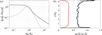
The overall behaviour of the decaying turbulence simulation is depicted in figure 2. First, figure 2(a) shows the evolution of the volume-averaged kinetic energy
 $\overline{q}$
and dissipation rate
 $\overline{\unicode[STIX]{x1D700}}$
. The evolution is very similar to that reported for decaying isotropic homogeneous turbulence, with an initial transient to a maximum
 $\overline{\unicode[STIX]{x1D700}}$
at approximately one eddy turnover time (i.e.
 $t\approx L_{0}/u_{0}$
). After dissipation peaks, the rates of decay observed for
 $\overline{q}$
and
 $\overline{\unicode[STIX]{x1D700}}$
are qualitatively similar to those reported for Mansour & Wray (Reference Mansour and Wray1994) and others. The Taylor Reynolds number is reasonably constant after the peak of dissipation, with a value of about
 $Re_{\unicode[STIX]{x1D706}}\approx 70$
for
 $tu_{0}/L_{0}\in [2-4]$
. In that same time period, the instantaneous integral length scale at the isotropic core,
 $L_{i}(t)$
, increases from
 $0.7L_{0}$
to
 $1.1L_{0}$
in a manner roughly proportional to the square root of the time (a detailed definition of
 $L_{i}$
can be found in appendix A, equation (A 1)).
The differences between the turbulence at the core and the turbulence near the boundaries are shown in figure 2(b), which reports vertical profiles of the horizontal and vertical kinetic energies,
 $q_{h}=\langle u^{2}+v^{2}\rangle /2$
and
 $q_{v}=\langle w^{2}\rangle /2$
, respectively (brackets denote horizontal averages). Note that the profiles are normalized with the volume-averaged kinetic energy at each time, so that even if
 $q_{h}/\overline{q}$
and
 $q_{v}/\overline{q}$
seem to grow at some locations,
 $q_{h}/u_{0}^{2}$
and
 $q_{v}/u_{0}^{2}$
decay essentially everywhere. It is interesting to note that, despite the anisotropy at the boundaries, turbulence is approximately isotropic in the interior region, where
 $q_{v}\approx q_{h}/2$
. On the other hand, while
 $q_{v}$
tends smoothly to zero at the boundaries, the horizontal kinetic energy shows strong peaks near the no-slip boundary and at the free-shear boundary. This behaviour is qualitatively consistent with that observed in other numerical simulations (Perot & Moin Reference Perot and Moin1995; Calmet & Magnaudet Reference Calmet and Magnaudet2003; Campagne et al.
Reference Campagne, Cazalbou, Joly and Chassaing2009; Herlina & Wissink Reference Herlina and Wissink2014).
(a) Time evolution of the volume-averaged kinetic energy
 $\overline{q}$
(——) and dissipation rate
 $\overline{\unicode[STIX]{x1D700}}$
(– – –, blue). (b) Profiles of the horizontal
 $q_{h}$
(——) and vertical
 $q_{v}$
(– – –, red) kinetic energies averaged on horizontal planes, normalized with the volume-averaged kinetic energy
 $\overline{q}$
. Lines correspond to
 $tu_{0}/L_{0}=1,2,3$
and
 $4$
. Time increases from thinner to thicker lines.

(a) Detail of the vertical profiles of the horizontal
 $q_{h}/\overline{q}$
(——) and vertical
 $q_{v}/\overline{q}$
(– – –) kinetic energies, and their ratio
 $2q_{v}/q_{h}$
(

 $\langle \unicode[STIX]{x1D700}\rangle$
(– – –),
 $-\unicode[STIX]{x2202}_{z}\unicode[STIX]{x1D6F7}$
(——),
 $\unicode[STIX]{x2202}_{t}q$
(

 $\unicode[STIX]{x1D6F1}$
(

 $tu_{0}/L_{0}=2,3$
and
 $4$
. Time increases from thinner to thicker lines.

The details of the profiles of the horizontal and vertical components of the kinetic energy near the stress-free surface are better appreciated in figure 3(a). Note that the distance from the top boundary,
 $z_{t}=2\unicode[STIX]{x03C0}L_{0}-z$
, is normalized with the integral scale measured in the isotropic region,
 $L_{i}$
, defined in (A 1). Also, the results are plotted with a reversed vertical axis, so that the stress-free surface is towards the top of the figure. The collapse of
 $q_{v}/\overline{q}$
for different times is remarkable, showing that the blockage region (where the vertical velocity is forced to zero by the boundary) extends to about one integral length scale in depth, consistent with Brumley & Jirka (Reference Brumley and Jirka1987) and others. On the other hand, the horizontal kinetic energy increases through this layer, peaking at the boundary at a value that increases slowly with time. Below
 $z_{t}\lesssim 0.01L_{i}$
, the horizontal kinetic energy
 $q_{h}$
is approximately constant, as expected within the viscous sublayer (Teixeira & Belcher Reference Teixeira and Belcher2000). Note that, according to the Hunt/Graham framework, the thickness of the viscous sublayer should scale as
 $\unicode[STIX]{x1D6FF}_{v}\approx \sqrt{\unicode[STIX]{x1D708}t}$
. However, in figure 3(a) the extent of the region where
 $q_{h}$
is constant near the free surface (i.e. the viscous sublayer
 $\unicode[STIX]{x1D6FF}_{v}$
) seems to scale with
 $L_{i}$
. This is a consequence of
 $L_{i}$
growing in time as
 $t^{1/2}$
, as mentioned earlier. In other words, for the present simulation, the ratio
 $\unicode[STIX]{x1D6FF}_{v}/L_{i}$
remains constant in the range of times analysed here.
The growth of
 $q_{h}$
within the blockage region agrees with the theory of Hunt & Graham (Reference Hunt and Graham1978), as well as with the simulation results of Perot & Moin (Reference Perot and Moin1995). However, the ratio between the horizontal kinetic energy at the boundary and in the isotropic region in our simulations is approximately 2, somewhat larger than the value of
 $3/2$
predicted by the inviscid theory of Hunt & Graham (Reference Hunt and Graham1978), the value of
 ${\approx}1.3$
predicted by the viscous theory of Teixeira & Belcher (Reference Teixeira and Belcher2000), or the value of
 ${\approx}1.75$
observed in other simulations. The reason of this discrepancy is not clear, although is possible that it might be related to the development of very large horizontal motions in the present case, at scales that were not resolved in previous simulations nor considered in the theories. For reference, figure 3(a) also includes the ratio of
 $2q_{v}/q_{h}$
.
Longitudinal and transverse one-dimensional spectra of the velocity for
 $tu_{0}/L_{0}=0,1,2$
and 4 (from thin to thick). (a) Stress-free surface,
 $z_{t}/L_{0}=0$
. (b) Isotropic region,
 $z_{t}/L_{0}=\unicode[STIX]{x03C0}$
. In both panels, line types are as follows:
 $E_{uu}(k_{x})$
(——),
 $E_{vv}(k_{x})$
(– – –, red) and
 $0.5\langle \unicode[STIX]{x1D700}\rangle ^{2/3}k_{x}^{-5/3}$
(– – –, black). The black circles indicate the wavenumber corresponding to the integral scale in the isotropic region,
 $L_{i}(t)$
.

Figure 3(b) shows the terms of the balance equation for the horizontally averaged kinetic energy
 $q=q_{h}+q_{v}$
,
 $$\begin{eqnarray}\unicode[STIX]{x2202}_{t}q=-\unicode[STIX]{x2202}_{z}\unicode[STIX]{x1D6F7}+\langle \unicode[STIX]{x1D700}\rangle ,\end{eqnarray}$$
where
 $\unicode[STIX]{x1D6F7}=\langle u_{i}^{2}w/2-\unicode[STIX]{x1D708}\unicode[STIX]{x2202}_{z}q+pw\rangle$
includes the vertical fluxes (advection, diffusion and pressure) and
 $\langle \unicode[STIX]{x1D700}\rangle$
is the horizontally averaged dissipation rate. The subindex
 $i$
in the definition of
 $\unicode[STIX]{x1D6F7}$
indicates a summation over the three velocity components. The figure also shows the pressure strain term
 $\unicode[STIX]{x1D6F1}=-\langle p\unicode[STIX]{x2202}_{z}w\rangle$
, which represents the energy transfer from the vertical component of the velocity to the horizontal components. All terms in the figure are normalized with
 $\langle \unicode[STIX]{x1D700}\rangle$
evaluated in the isotropic region. It can be observed that, of all the terms in (4.1), dissipation is dominant throughout the whole layer. However, for
 $z_{t}\lesssim 0.02L_{i}$
the vertical fluxes and the pressure–strain become important. The net effect of the former is to remove energy from the horizontal velocity component, while the pressure–strain acts like a source, removing energy from the vertical velocity component (Perot & Moin Reference Perot and Moin1995). In the rest of the blockage layer, the pressure–strain term is slightly negative, which indicates a (weaker) transfer of energy from horizontal to vertical motions. This latter transfer represents the normal behaviour of
 $\unicode[STIX]{x1D6F1}$
, acting to maintain isotropy in the turbulent flow (return-to-isotropy term). The profiles of
 $\unicode[STIX]{x1D6F1}$
shown in figure 3(b) are consistent with those reported in previous works, e.g. Perot & Moin (Reference Perot and Moin1995) or Aronson et al. (Reference Aronson, Johansson and Löfdahl1997).
4.1 One-dimensional energy spectra near the shear-free surface
We now turn our attention to the horizontal spectra of the various components of the kinetic energy, and their comparison with the field measurements given in figure 1 and the results for stratified turbulence. Examining figure 3, it seems that the conditions for stratified-like turbulence are met relatively close to the free-shear surface (say, for
 $z_{t}\lesssim 0.1L_{i}$
): the vertical velocity is much smaller than the horizontal components and the dissipation is dominant in (4.1). It is unclear to what extent the conditions are met in the viscous sublayer (
 $z_{t}\lesssim 0.01L_{i}$
), where
 $\unicode[STIX]{x2202}_{z}\unicode[STIX]{x1D6F7}$
and
 $\unicode[STIX]{x1D6F1}$
are not negligible small. Note also that this is only a first indication, since figure 3(b) does not provide information on the horizontal wavelengths where energy is gained or lost, which will be analysed below.
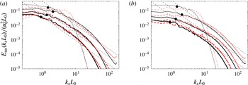
Figure 4 shows a time sequence of the one-dimensional spectra in
 $k_{x}$
of the horizontal components of the velocity,
 $E_{uu}(k_{x}L_{0})$
and
 $E_{vv}(k_{x}L_{0})$
, both at the stress-free boundary and in the isotropic region. At time
 $t=0$
, the spectra in both locations are fairly narrow, reflecting the initialization method. As time evolves, however, the spectra fill out at higher wavenumbers, as energy is transferred downscale. By approximately
 $t=2L_{0}/u_{0}$
, an approximate
 $k_{x}^{-5/3}$
spectrum has developed at the free surface (figure 4
a), which is maintained for later times. Also, the longitudinal and transverse spectra collapse onto a single line at the free-shear surface, as in the experimental data (see figure 1).
On the other hand, in the isotropic region (figure 4
b), the spectrum takes a form more typical of a moderate Reynolds number isotropic turbulent flow. In particular, it does not exhibit
 $k_{x}^{-5/3}$
behaviour at intermediate scales and the values of the longitudinal and transverse spectra differ for large scales. Clearly the presence of the stress-free boundary is causing this difference in behaviour.
Longitudinal and transverse one-dimensional spectra of the velocity for
 $tu_{0}/L_{0}=2$
(thin) and 4 (thick), at two different distances from the free surface. (a)
 $z_{t}=0.088L_{0}$
, corresponding to
 $z_{t}/L_{i}=0.123$
and
 $0.083$
. (b)
 $z_{t}=0.035L_{0}$
, corresponding to
 $z_{t}/L_{i}=0.049$
and
 $0.033$
. In both panels, line types are as follows:
 $E_{uu}(k_{x})$
(——),
 $E_{vv}(k_{x})$
(– – –, red),
 $E_{ww}(k_{x})$
(

 $0.5\langle \unicode[STIX]{x1D700}\rangle ^{2/3}k_{x}^{-5/3}$
(– – –, black). The blue vertical line indicates
 $k_{x}=1/z_{t}$
, and the black circles indicate the wavenumber corresponding to the integral scale in the isotropic region,
 $L_{i}(t)$
.

The behaviour observed in 4(a) is not only characteristic of the stress-free boundary, but of the layer
 $z_{t}/L_{i}\lesssim 0.1$
where the conditions for stratified-like turbulence are met. This is shown in figure 5, where the spectra of all three velocity components at two locations below
 $0.1L_{i}$
are plotted. Figure 5(a) corresponds to a position farther from the boundary (
 $z/L_{i}\approx 0.083-0.123$
), while figure 5(b) corresponds to a position closer to the boundary (
 $z/L_{i}\approx 0.033-0.049$
). The dashed lines correspond to
 $E_{uu}=C_{1}\langle \unicode[STIX]{x1D700}\rangle ^{2/3}k^{-5/3}$
, where
 $\langle \unicode[STIX]{x1D700}\rangle$
is evaluated at each
 $z_{t}$
and
 $C_{1}=0.5$
.
For wavenumbers smaller than
 $1/z_{t}$
(indicated with a blue vertical line in figure 5), the vertical velocity becomes much smaller than the horizontal velocities, as first noted by Hunt & Graham (Reference Hunt and Graham1978). Note that
 $z_{t}$
plays the role of
 $\unicode[STIX]{x1D6FF}$
in the hypothesis put forward in § 1, hence these are horizontal scales that are large compared to the distance to the free surface. The horizontal velocity spectra exhibit a clear
 $-5/3$
range for these wavenumbers, extending up to wavenumbers of the order of
 $1/L_{i}$
(indicated by black circles in figure 5). Note that the
 $k^{-5/3}$
range cannot be due to a Kolmogorov-like turbulence, since the hypothesis for an inertial Kolmogorov range are not met in this wavenumber range (i.e. the flow is not homogeneous nor isotropic). Interestingly, in the
 $-5/3$
range
 $E_{uu}(k_{x})$
and
 $E_{vv}(k_{x})$
have approximately the same value, consistently with the field data (figure 1) and with stratified turbulence (Lindborg Reference Lindborg2006). This collapse of the longitudinal and transverse spectra is a consequence of an approximate equipartition between the rotational and divergent energy, a characteristic feature of stratified-like turbulence (Lindborg & Brethouwer Reference Lindborg and Brethouwer2007; Lindborg Reference Lindborg2015). Although not shown here, for the present simulations the ratio between the rotational and divergent energy spectrum is
 ${\approx}1$
for large scales (
 $k_{x}L_{0}\lesssim 10$
) in the region close to the free surface (
 $z_{t}\lesssim 0.1L_{i}$
), while in the isotropic core it is approximately
 ${\approx}3$
.
Finally, for
 $k_{x}\gtrsim 1/z_{t}$
, the spectra in figure 5(a,b) show that the two transverse spectra
 $E_{vv}(k_{x})$
and
 $E_{ww}(k_{x})$
are approximately the same, while the longitudinal component
 $E_{uu}(k_{x})$
is somewhat smaller. This behaviour is consistent with a more isotropic turbulence at length scales smaller than the distance from the boundary, in agreement with our hypothesis. Note that, in homogeneous and isotropic turbulence, the assumption of a power-law spectrum of the form
 $E_{uu}(k_{x})\sim k^{-p}$
yields
 $E_{vv}(k_{x})=E_{ww}(k_{x})=0.5(1+p)E_{uu}(k_{x})$
(Pope Reference Pope2000, ch. 6.5.1), which for
 $p=5/3$
results in
 $E_{vv}(k_{x})=E_{ww}(k_{x})=1.33E_{uu}(k_{x})$
.
As mentioned in the introduction, Herlina & Jirka (Reference Jirka2008) show a similar behaviour for the frequency spectrum of the horizontal and vertical velocities in the vicinity of a stress-free boundary. The vertical velocity spectrum is progressively damped at low frequencies as the free surface is approached. Interestingly, they do show a
 $-5/3$
slope for higher Reynolds numbers, but in their paper they do not comment on that, except to say that the vertical fluctuation components are inhibited by the surface, whereas the horizontal fluctuations may develop freely.
4.2 Further considerations: scale-by-scale budget and vertical shearing
The
 $-5/3$
behaviour depicted in figures 4 and 5 is observed for several eddy turnover times during the decay of the flow, and it suggests that turbulence near a free surface retains some of the properties of stratified turbulence. As explained in the introduction, our hypothesis is that the emergence of the
 $-5/3$
range occurs in regions of the flow where vertical motions are constrained for some scales (
 $k_{x}\lesssim 1/z_{t}$
). There, if a forward cascade into the dissipation range occurs, dimensional arguments suggest an inertial range. It was also postulated that, for the larger-scale motions, the vertical shearing will be increased. This would lead to shear instabilities and an enhanced mechanism for forward cascade, even given the suppression of the vertical motions by the stress-free surface. The results of the previous subsection have shown evidence of some of these behaviours, in particular the
 $-5/3$
inertial range for
 $1/L_{i}\lesssim k_{x}\lesssim 1/z_{t}$
and of the recovery of a more isotropic spectrum at scales smaller than the distance to the stress-free surface,
 $k_{x}\gtrsim 1/z_{t}$
. In the present subsection we will examine the spectral energy equation, along with the enhancement of the vertical shearing.
Scale-by-scale horizontal kinetic energy budget at
 $tu_{0}/L_{0}=2$
. (a)
 $z_{t}=0.035L_{0}=0.049L_{i}$
. (b)
 $z_{t}=0$
. In both panels, line types are:
 $k_{h}^{5/3}E_{h}(k_{h})/\langle \unicode[STIX]{x1D700}\rangle ^{2/3}$
(——);
 $k_{h}D(k_{h})/\langle \unicode[STIX]{x1D700}\rangle$
(

 $k_{h}T_{\unicode[STIX]{x1D6F1}}(k_{h})/\langle \unicode[STIX]{x1D700}\rangle$
(

 $k_{h}T(k_{h})/\langle \unicode[STIX]{x1D700}\rangle$
(– – –). The blue vertical line in (a) indicates
 $k_{h}=1/z_{t}$
.

Figure 6 shows a scale-by-scale analysis, near the free surface, of the spectral energy equation
 $$\begin{eqnarray}\unicode[STIX]{x2202}_{t}E_{h}(k_{h})=T(k_{h})+T_{\unicode[STIX]{x1D6F1}}(k_{h})+D(k_{h}),\end{eqnarray}$$
which is obtained by adding the momentum equations for
 $u$
and
 $v$
in Fourier space (horizontal transforms only) after multiplication by the complex conjugate of the corresponding Fourier coefficients of the velocity. Note that now it is more convenient to work with the horizontal wavenumber magnitude,
 $k_{h}=\sqrt{k_{x}^{2}+k_{y}^{2}}$
rather than
 $k_{x}$
. The mathematical definition of the terms in (4.2) can be found in appendix A, but from a physical point of view they are the horizontal kinetic energy spectrum
 $E_{h}(k_{h})$
, the spectrum of the pseudo-dissipation
 $D(k_{h})$
, the spectrum of the pressure–strain
 $T_{\unicode[STIX]{x1D6F1}}(k_{h})$
and a transfer spectrum
 $T(k_{h})$
(a detailed description of the pseudo-dissipation and its relationship with the dissipation can be found in Pope (Reference Pope2000), but for the purpose of the present analysis they are essentially equivalent). The latter includes the effect of both local spectral (inter-scale) transfer and the vertical transport of energy due to the inhomogeneity of the flow (the vertical flux term,
 $\unicode[STIX]{x1D6F7}$
, in (4.1)).
Note that in figure 6 the horizontal kinetic energy spectrum
 $E_{h}(k_{h})$
is plotted premultiplied by
 $k_{h}^{5/3}$
(compensated spectrum), in order to visualize the wavenumber range where a
 $-5/3$
spectrum is obtained. The rest of the terms are normalized with the horizontally averaged dissipation,
 $\langle \unicode[STIX]{x1D700}\rangle$
, and premultiplied by
 $k_{h}$
, so that the area under the curve for a given wavenumber range corresponds to the actual energy content of the range.
Figure 6(a) shows the balance at approximately
 $z_{t}\approx 0.05L_{i}$
and at time
 $tu_{0}/L_{0}=2$
. The pressure–strain spectrum
 $T_{\unicode[STIX]{x1D6F1}}(k_{h})$
shows that energy is transferred from vertical to horizontal motions at large scales, while the opposite occurs at small scales. Overall, the amount of energy transferred from vertical to horizontal components is small compared to
 $D(k_{h})$
, and indeed the integral of
 $T_{\unicode[STIX]{x1D6F1}}(k_{h})$
in figure 6(a) is close to zero (see also figure 3
b). On the other hand,
 $T(k_{h})$
is comparable to
 $D(k_{h})$
, removing energy from the large scales and transferring it to smaller scales (forward cascade). Note that
 $T(k_{h})$
does not show a zero range at wavenumbers where the compensated spectra exhibit a
 $-5/3$
range, as would be expected for the three-dimensional transfer spectrum for isotropic turbulence (see, e.g. Pope Reference Pope2000). The reasons for this behaviour are an insufficient scale separation (i.e. the Reynolds number of the simulation is limited,
 $Re_{\unicode[STIX]{x1D706}}\approx 70$
), as well as the fact that
 $T(k_{h})$
is aliased in the vertical direction: since the terms in (4.2) are defined from Fourier transformations in the horizontal plane only, a given horizontal wavenumber
 $k_{h}$
has contributions from all scales in the vertical direction (see Tennekes & Lumley Reference Tennekes and Lumley1972, ch. 8.1).
While figure 6(a) shows an energy balance with a forward cascade to smaller scales to be dissipated, the picture for the free-shear surface (see figure 6
b) is less clear. Although the overall behaviour shown in figures 6(a) and 6(b) is qualitatively similar, the effect of the vertical flux is more pronounced at
 $z_{t}=0$
than below the free surface. Note that in figure 6(b) the integral of
 $T(k_{h})$
is clearly negative, and approximately of the same order as the pseudo-dissipation. This suggests that the vertical fluxes are more important at the free surface than below, removing energy mostly from the large scales. Also, the pressure–strain transfer is stronger at
 $z_{t}$
, with a net positive value (indicating a net transfer from vertical to horizontal velocities, as discussed previously in figure 3
b).
Another interesting comparison between figures 6(a) and 6(b) is the value of the plateau in the compensated horizontal energy spectra. The constant in the energy spectra seems to be slightly larger at the free surface than beneath it, consistently with the one-dimensional spectra in figures 4 and 5. Although not shown in the figure, the level of the plateau also changes slightly with time, increasing as the overshoot at the high wavenumber range of the plateau shifts to the left. In any case, the value of the constant lies in the range 0.75–1 (shown with blue horizontal lines in figure 6) for times in the range
 $2\lesssim tu_{0}/L_{0}\lesssim 4$
and
 $z_{t}\lesssim 0.1L_{i}$
. This value is reasonably close to the value obtained in the isotropic part of the domain (not shown here), as well as the value estimated for
 $E_{h}(k_{h})$
in isotropic, homogeneous, three-dimensional turbulence (see appendix B). This is in agreement with the results of Chickadel et al. (Reference Chickadel, Talke, Horner-Devine and Jessup2011), since in figure 1 the
 $-5/3$
slope regions appear to be co-linear in the isotropic and anisotropic ranges of the spectra. Note also that this value is much smaller than the typical values of 5–6 obtained for two-dimensional turbulence forced at small scales (Maltrud & Vallis Reference Maltrud and Vallis1991), a flow configuration in which two-dimensional motions exhibit an inertial range.
(a) Root-mean-square of the gradients of the horizontal velocity, normalized with the value in the isotropic region, at times
 $tu_{0}/L_{0}=1,2$
and 4.
 $\langle (\unicode[STIX]{x2202}_{y}u)^{2}\rangle$
(– – –);
 $\langle (\unicode[STIX]{x2202}_{z}u)^{2}\rangle$
(

 $z_{t}=0.035L_{0}$
. The upper group of lines is
 $tu_{0}/L_{0}=2$
, corresponding to
 $z_{t}/L_{i}=0.033$
. The lower group is
 $tu_{0}/L_{0}=4$
and
 $z_{t}/L_{i}=0.049$
.
 $E_{\unicode[STIX]{x2202}_{y}u}(k_{x})$
(– – –);
 $E_{\unicode[STIX]{x2202}_{z}u}(k_{x})$
(

 $E_{\unicode[STIX]{x2202}_{y}u}(k_{x})=E_{\unicode[STIX]{x2202}_{z}u}(k_{x})$
in the isotropic region (——). The blue vertical line indicates
 $k_{x}=1/z_{t}$
.

The second hypothesis (increased vertical shearing) is tested in figure 7, which shows the behaviour of the transverse gradients (horizontal and vertical) of the horizontal velocity. First, figure 7(a) shows the vertical profiles of the r.m.s. of the transverse gradients of the horizontal velocity, normalized with the values in the isotropic region. It is possible to observe that within the blockage region (
 $z_{t}\lesssim L_{i}$
), the r.m.s. of the transverse horizontal gradient (
 $\langle (\unicode[STIX]{x2202}_{y}u)^{2}\rangle$
, in red) decreases slightly with respect to its value on the isotropic region. However, the vertical shear (
 $\langle (\unicode[STIX]{x2202}_{z}u)^{2}\rangle$
, in blue) is enhanced by a factor of approximately 1.5, peaking at approximately
 $z_{t}\approx 0.02-0.04L_{i}$
. Closer to the free surface, the vertical gradients of horizontal velocities go to zero, with a reduction in the fluctuations of approximately 50 % at about
 $z_{t}\approx 0.01L_{i}$
. Note that, within the viscous sublayer (namely,
 $z_{t}\lesssim 0.01L_{i}$
), figure 3(a) shows that the horizontal velocity fluctuations plateau while the vertical velocities are essentially zero, which together with the results in figure 7(a) suggest that the horizontal velocities do not vary much with
 $z_{t}$
inside this viscous sublayer.
To determine whether the results of the present simulation are consistent with the scaling arguments presented in the introduction, and in particular whether the ratio
 $L/\unicode[STIX]{x1D6FF}$
is large, we can use the depth where the vertical shear is the strongest, i.e. where the hypothesized effects are the strongest. This depth is approximately at
 $z_{t}/L_{i}=0.03$
. Identifying
 $L_{i}$
with
 $L$
and
 $z_{t}$
with
 $\unicode[STIX]{x1D6FF}$
, then we find that
 $L/\unicode[STIX]{x1D6FF}\doteq 33$
. While this number is not as large as for the field data, it appears to be large enough for a somewhat narrow inertial-like range to develop, as shown in figures 4 and 5.
The scales responsible for the peak in
 $\langle (\unicode[STIX]{x2202}_{z}u)^{2}\rangle$
are evaluated in figure 7(b), which shows the spectra of the vertical and horizontal gradients of the horizontal velocities (
 $E_{\unicode[STIX]{x2202}_{z}u}(k_{x},z)$
and
 $E_{\unicode[STIX]{x2202}_{y}u}(k_{x},z)$
, defined in appendix A) at approximately the position where
 $\langle (\unicode[STIX]{x2202}_{z}u)^{2}\rangle$
is maximum. It can be observed that for scales larger than the distance to the free-shear surface (
 $k_{x}\lesssim 1/z_{t}$
), the vertical shear is enhanced (
 $E_{\unicode[STIX]{x2202}_{z}u}$
, in blue) with respect to the values in the isotropic region (in black). On the other hand, the horizontal gradients (
 $E_{\unicode[STIX]{x2202}_{y}u}$
, in red) associated with large scales are smaller than in the isotropic region. At smaller scales, as the flow becomes more isotropic,
 $E_{\unicode[STIX]{x2202}_{y}u}$
and
 $E_{\unicode[STIX]{x2202}_{z}u}$
tend to collapse, as it can be clearly observed in the upper group of lines in figure 7(b).
The increase in vertical shearing shown in figure 7 is consistent with the predictions for stratified turbulence by Lilly (Reference Lilly1983) and Billant & Chomaz (Reference Billant and Chomaz2001), and with the simulations of Riley & de Bruyn Kops (Reference Riley and de Bruyn Kops2003). Together with the downscale transfer shown in figure 6 and the inertial ranges in figures 4 and 5, it suggests that the dynamical model of stably stratified turbulence is relevant to turbulence near shear-free surfaces.
5 Conclusions
We hypothesize that the turbulence dynamics very near the river surface observed in experiments is very similar to that for strongly stratified turbulent flows. In particular, very near the surface, the vertical velocity is suppressed by the presence of the surface, modifying the turbulence dynamics. Due to nonlinear dynamics, however, strong vertical shearing of the horizontal velocity can develop, which results in shear instabilities and three-component turbulence at much smaller scales. If the separation of the horizontal energy-containing scale from the instability scale is large enough, this results in a downscale energy transfer that depends only on the kinetic energy dissipation rate. Dimensional analysis then leads to the
 $k_{h}^{-5/3}$
spectral behaviour.
In order to test the hypothesis, we have performed a DNS of incompressible, decaying turbulence near a stress-free surface. Our simulation results are consistent with the hypothesis and with the field data, exhibiting a
 $k_{h}^{-5/3}$
behaviour near the stress-free boundary over approximately one decade in wavenumber, while the flow displays a spectrum more characteristic of low Reynolds isotropic turbulence in the flow interior. Moreover, in a layer sufficiently close to the free surface, the other characteristics of stratified-like turbulence are present. Namely, the vertical shearing is enhanced for large scales, and there is a forward cascade dominated by the local dissipation.
However, at the free surface these conditions are not completely satisfied: by construction, the vertical gradient of the horizontal velocity is zero at
 $z_{t}=0$
. Also, even if a forward cascade is apparent, the contribution from the vertical transport of energy is of the same order of magnitude as the dissipation. Our conjecture is that the behaviour of the large scales at the free surface is driven by the behaviour of the large scales just below, in a layer within the blockage layer but outside of the viscous sublayer (
 $0.01\lesssim z_{t}/L_{i}\lesssim 0.1$
at the present Reynolds numbers). Note that
 $\unicode[STIX]{x2202}_{z}u\approx 0$
in the viscous sublayer, and hence the horizontal motions at large scales at approximately
 $z_{t}\approx 0.01L_{i}$
must be mimicked by the large-scale horizontal motions at the free surface.
It is important to highlight the novelty of the application of the stratified turbulence analogy to the turbulence near a shear-free surface. The analogy suggests that the
 $-5/3$
range is an intrinsic property of this layer, not a consequence of a spectrum imposed from the outer region. This is an important difference with respect to Hunt/Graham theory, where the spectrum at the free surface is obtained as a modification of the spectrum in the outer region. Also, the present model links the structure of the large scales to the dissipation of the small scales, through the
 $-5/3$
law. This might be the explanation of the apparent discrepancy between some of the models for gas transfer in air–liquid interfaces (Moog & Jirka Reference Moog and Jirka1999 versus Magnaudet & Calmet Reference Magnaudet and Calmet2006).
The results also support the suggestion by Chickadel et al. (Reference Chickadel, Talke, Horner-Devine and Jessup2011) that the turbulence properties of near-surface turbulent flow can be determined remotely, and give some rationale as to why this is the case. Since the mechanism underlying the spectral slope is different, it is reasonable to expect that there may also be a difference between the proportionality constants for the isotropic and the near-surface anisotropic cases. The present results however, suggest that this is not the case, and that the value of the constants are roughly the same.
Finally, one might expect similar behaviour for other flows where one component of the velocity is inhibited. Examples of this could include flows in rivers and estuaries when the horizontal energy-containing scales are much larger than the fluid depth (Yokosi Reference Yokosi1967), and in stably stratified flows with regions of local, large density gradients (Salehipour, Caulfield & Peltier Reference Salehipour, Caulfield and Peltier2016).
Acknowledgements
The authors thank S. M. de Bruyn Kops for valuable discussions of simulating strongly stratified flows. This work was supported by ARO grant no. W911NF-08-1-0155. O.F. was partly supported by the Spanish Ministry of Economy and Competitiveness, under grant TRA2012-37714.
Appendix A. Definition of spectral quantities
The integral length scale measured in the isotropic region is defined as
 $$\begin{eqnarray}L_{i}(t)=\frac{1}{z_{2}-z_{1}}\int _{z_{1}}^{z_{2}}\frac{3\unicode[STIX]{x03C0}}{4}\frac{\displaystyle \iint (\hat{u} \hat{u} ^{\ast }+\hat{v}\hat{v}^{\ast }+{\hat{w}}{\hat{w}}^{\ast })(k_{x}^{2}+k_{y}^{2})^{-1/2}\,\text{d}k_{x}\,\text{d}k_{y}}{\displaystyle \iint (\hat{u} \hat{u} ^{\ast }+\hat{v}\hat{v}^{\ast }+{\hat{w}}{\hat{w}}^{\ast })\,\text{d}k_{x}\,\text{d}k_{y}}\,\text{d}z,\end{eqnarray}$$
where
 $\hat{u} ,\hat{v}$
and
 ${\hat{w}}$
are the Fourier coefficients of the three velocity components, functions of the horizontal wavenumbers (
 $k_{x}$
and
 $k_{y}$
) and the vertical coordinate
 $z$
. The asterisk denotes complex conjugate, and the integrals in
 $k_{x}$
and
 $k_{y}$
extend to the whole range of wavenumbers. In the vertical direction, the integral length scale is averaged between
 $z_{1}/L_{0}=\unicode[STIX]{x03C0}/2$
to
 $z_{2}/L_{0}=3\unicode[STIX]{x03C0}/2$
, a region of the computational domain where the flow is shown to be roughly isotropic flow (see figure 2
b).
The horizontal kinetic energy spectrum
 $E_{h}(k_{h})$
is defined as the spectral energy density of the horizontal kinetic energy at horizontal wavenumber
 $k_{h}$
,
 $$\begin{eqnarray}E_{h}(k_{h},z)=\int _{-\infty }^{\infty }\int _{-\infty }^{\infty }\frac{\hat{u} \hat{u} ^{\ast }+\hat{v}\hat{v}^{\ast }}{2}\unicode[STIX]{x1D6FF}\left(k_{h}-\sqrt{k_{x}^{\prime 2}+k_{y}^{\prime 2}}\right)\,\text{d}k_{x}^{\prime }\,\text{d}k_{y}^{\prime },\end{eqnarray}$$
where
 $\unicode[STIX]{x1D6FF}$
is the Dirac function and the integrals in
 $k_{x}^{\prime }$
and
 $k_{y}^{\prime }$
extend to the whole range of wavenumbers.
The spectrum of the pseudo-dissipation of horizontal kinetic energy is defined as
 $$\begin{eqnarray}D(k_{h},z)=\unicode[STIX]{x1D708}\int _{-\infty }^{\infty }\int _{-\infty }^{\infty }(\widehat{\unicode[STIX]{x2202}_{j}u}\widehat{\unicode[STIX]{x2202}_{j}u}^{\ast }+\widehat{\unicode[STIX]{x2202}_{j}v}\widehat{\unicode[STIX]{x2202}_{j}v}^{\ast })\unicode[STIX]{x1D6FF}\left(k_{h}-\sqrt{k_{x}^{\prime 2}+k_{y}^{\prime }2}\right)\,\text{d}k_{x}^{\prime }\,\text{d}k_{y}^{\prime },\end{eqnarray}$$
where
 $\unicode[STIX]{x1D708}$
is the kinematic viscosity, the subindex
 $j$
indicates summation over the three spatial coordinates.
The spectrum of the pressure–strain transfer is defined as
 $$\begin{eqnarray}T_{\unicode[STIX]{x1D6F1}}(k_{h},z)=\int _{-\infty }^{\infty }\int _{-\infty }^{\infty }\text{Re}(\widehat{p}\,\widehat{\unicode[STIX]{x2202}_{z}w}^{\ast })\unicode[STIX]{x1D6FF}\left(k_{h}-\sqrt{k_{x}^{\prime 2}+k_{y}^{\prime 2}}\right)\,\text{d}k_{x}^{\prime }\,\text{d}k_{y}^{\prime },\end{eqnarray}$$
where
 $\hat{p}$
is the Fourier coefficient of the kinematic pressure and Re
 $(a)$
stands for the real part of the complex number
 $a$
.
The transfer spectrum,
 $T(k_{h},z)$
, is defined as
 $$\begin{eqnarray}\displaystyle T(k_{h},z) & = & \displaystyle \unicode[STIX]{x1D708}\unicode[STIX]{x2202}_{zz}E_{h}(k_{h},z)\nonumber\\ \displaystyle & & \displaystyle +\,\int _{-\infty }^{\infty }\int _{-\infty }^{\infty }\text{Re}(-\widehat{\unicode[STIX]{x2202}_{j}(u_{j}u)}\hat{u} ^{\ast }-\widehat{\unicode[STIX]{x2202}_{j}(u_{j}v)}\hat{v}^{\ast })\unicode[STIX]{x1D6FF}\left(k_{h}-\sqrt{k_{x}^{\prime 2}+k_{y}^{\prime 2}}\right)\,\text{d}k_{x}^{\prime }\,\text{d}k_{y}^{\prime },\qquad\end{eqnarray}$$
where the first term represents the viscous diffusion of
 $E_{h}(k_{h},z)$
, and the second term includes the local spectral transfer and the vertical turbulent transport of energy.
Note that, by definition
 $E_{h}(k_{h},z),D(k_{h},z),T_{\unicode[STIX]{x03C0}}(k_{h},z)$
and
 $T(k_{h},z)$
are all aliased with the vertical scales (Tennekes & Lumley Reference Tennekes and Lumley1972), in the sense of being able only to segregate the horizontal scales. Since
 $\hat{u}$
and
 $\hat{v}$
are functions of
 $z$
, at any given
 $z$
they have contributions from all possible wavelengths in the vertical direction.
From a numerical point of view,
 $E_{h}$
,
 $D$
and
 $T_{\unicode[STIX]{x1D6F1}}$
are computed evaluating the previous expressions, using 512 bins in
 $k_{h}$
to compute the cylindrical integrals. The time derivative of
 $E_{h}$
is then computed numerically, using a second-order approximation for the time derivative, and the transfer spectrum
 $T$
is obtained from (4.2).
Finally, the longitudinal one dimensional spectra of the transverse gradients in the vertical and horizontal directions are defined as
 $$\begin{eqnarray}E_{\unicode[STIX]{x2202}_{y}u}(k_{x},z)=\int _{-\infty }^{\infty }\widehat{\unicode[STIX]{x2202}_{y}u}\widehat{\unicode[STIX]{x2202}_{y}u}^{\ast }\,\text{d}k_{y}\end{eqnarray}$$
and
 $$\begin{eqnarray}E_{\unicode[STIX]{x2202}_{z}u}(k_{x},z)=\int _{-\infty }^{\infty }\widehat{\unicode[STIX]{x2202}_{z}u}\widehat{\unicode[STIX]{x2202}_{z}u}^{\ast }\,\text{d}k_{y}.\end{eqnarray}$$
Appendix B. Energy spectrum function versus horizontal spectrum
For homogeneous isotropic turbulence, Pope (Reference Pope2000) shows that the velocity spectrum tensor
 $\unicode[STIX]{x1D719}_{ij}(\boldsymbol{k})$
can be expressed as
 $$\begin{eqnarray}\unicode[STIX]{x1D719}_{ij}(\boldsymbol{k})=\frac{E(k)}{4\unicode[STIX]{x03C0}k^{2}}\left(\unicode[STIX]{x1D6FF}_{ij}-\frac{k_{i}k_{j}}{k^{2}}\right),\end{eqnarray}$$
where
 $E(k)$
is the energy spectrum function,
 $k$
is the modulus of the wavenumber vector
 $\boldsymbol{k}=(k_{x},k_{y},k_{z})$
, and
 $\unicode[STIX]{x1D6FF}_{ij}$
is the Kronecker delta. In terms of
 $\unicode[STIX]{x1D719}_{ij}$
, the horizontal kinetic energy spectrum defined in (A 2) can be expressed as
 $$\begin{eqnarray}E_{h}(k_{h})=\int \frac{1}{2}(\unicode[STIX]{x1D719}_{xx}(\boldsymbol{k})+\unicode[STIX]{x1D719}_{yy}(\boldsymbol{k}))\,\text{d}C(k_{h}),\end{eqnarray}$$
where
 $k_{h}=\sqrt{k_{x}^{2}+k_{y}^{2}}$
and
 $\int \text{d}C(k_{h})$
is an integral in a cylindrical shell of radius
 $k_{h}$
, extending in
 $k_{z}$
from
 $-\infty$
to
 $\infty$
. Introducing the expression of
 $\unicode[STIX]{x1D719}_{ij}$
in (B 2), and noting that the integrand is a function of
 $k_{h}$
and
 $k_{z}$
only, we obtain
 $$\begin{eqnarray}E_{h}(k_{h})=\frac{1}{2}\int _{-\infty }^{\infty }\frac{E((k_{h}^{2}+k_{z}^{2})^{1/2})}{4\unicode[STIX]{x03C0}(k_{h}^{2}+k_{z}^{2})}\left(2-\frac{k_{h}^{2}}{k_{h}^{2}+k_{z}^{2}}\right)2\unicode[STIX]{x03C0}k_{h}\,\text{d}k_{z}.\end{eqnarray}$$
Analytical integration of this equation without an explicit expression for
 $E(k)$
is not possible. Assuming that
 $E(k)=C\unicode[STIX]{x1D700}^{2/3}k^{-5/3}$
, equation (B 3) integrates to
 $E_{h}(k_{h})=C_{h}\unicode[STIX]{x1D700}^{2/3}k_{h}^{-5/3}$
, with
 $C_{h}=0.54C$
. For the usual value
 $C=1.5$
for homogeneous isotropic turbulence, this yields
 $C_{h}=0.8$
, very similar to the value of the plateau reported in figure 6.