




No CrossRef data available.
Article contents
Analysis of aggregation, a worked example: numbers of ticks on red grouse chicks
Published online by Cambridge University Press: 07 August 2001
Abstract
The statistical aggregation of parasites among hosts is often described empirically by the negative binomial (Poisson-gamma) distribution. Alternatively, the Poisson-lognormal model can be used. This has the advantage that it can be fitted as a generalized linear mixed model, thereby quantifying the sources of aggregation in terms of both fixed and random effects. We give a worked example, assigning aggregation in the distribution of sheep ticks Ixodes ricinus on red grouse Lagopus lagopus scoticus chicks to temporal (year), spatial (altitude and location), brood and individual effects. Apparent aggregation among random individuals in random broods fell 8-fold when spatial and temporal effects had been accounted for.
Keywords
Information
- Type
- Research Article
- Information
- Copyright
- 2001 Cambridge University Press
INTRODUCTION
Counts in ecological studies often show non-random, aggregated statistical distributions. Heterogeneity in the way parasites are dispersed among hosts, for example, may be due to genetic, physiological or behavioural differences among individuals and may also vary in time and space (Shaw & Dobson, 1995). In general, to understand and model parasite aggregation, it is helpful to quantify the contribution of each separate source of aggregation to the total aggregation observed.
One approach has been to model the presumed causes of aggregation and to compare model output with laboratory and field measures of aggregation (Grenfell et al. 1995). Another has been to devise indices that partition parasite aggregation at 2 hierarchical levels in the host population (Boulinier et al. 1996). A statistical modelling approach to the problem is to partition variations in counts according to a set of putative explanatory effects, much as one partitions variance in the dependent variable in analysis of variance and covariance. Here, we develop a method for doing this, using counts of ticks Ixodes ricinus on chicks of red grouse Lagopus lagopus scoticus as an example.
The Poisson distribution is the mathematical embodiment of randomness and plays a central role in analyses of counts in ecology. Specifically, if n parasites occur at random on N hosts, then the distribution of numbers of parasites per host will be approximately Poisson. As N becomes very large and the mean number of parasites per host remains the same (n, N→∞, with n/N = μ fixed), the approximation becomes exact. This is convenient for the statistical analysis of counts: the Poisson distribution is a member of the exponential family and so, when the mean counts are covariate-dependent, their dependency can be modelled by fitting a generalized linear model (McCullagh & Nelder, 1989).
Exploratory analysis of counts often begins with an assessment of the hypothesis of randomness. As the mean and variance of the Poisson distribution are equal, this assessment often takes the form of calculating a variance/mean ratio: values greater than 1 suggest more variation than random and are called over-dispersed, aggregated or clumped; values smaller than 1 suggest less variation than random, and are called under-dispersed or regular.
Counts that are the outcome of several random processes may or may not be Poisson. The sum of several independent Poisson variables remains Poisson, but a multiple of a Poisson variable is not Poisson. In nature, therefore, factors that affect multiplicative processes such as reproduction are likely to give rise to aggregated distributions.
Disproving randomness is not an end in itself, but leads to further analysis. In some situations, this may be a comparison of the levels of non-randomness in different populations using aggregation indices. Here, the choice of index is crucial when comparing populations with different mean intensities, particularly when one wants an index that does not vary with the mean (Pielou, 1977). If so, the index I = (V/m)−1 is appropriate for situations in which we expect the variance V to be proportional to the mean m. An alternative index is needed when we expect the variance to increase as the square of the mean. The index I/m = (V−m)/m2 is widely used for this purpose, and is equal to the inverse of the parameter k from the negative binomial distribution. Thus, even in the selection of aggregation indices, some element of modelling and an understanding of the mechanisms generating the data are inescapable.
In ecology, the most widely used distribution for the mean that meets the assumption of the variance being proportional to the square of the mean is the gamma distribution, which leads to a negative binomial (Poisson-gamma) distribution for the counts. Thus many models of host–parasite dynamics contain as a measure of aggregation the parameter k from the negative binomial distribution. Parasites are typically found aggregated among hosts (Shaw & Dobson, 1995) and if host mortality depends on parasite burden, then greater parasite aggregation (smaller k) leads to greater stability in host population density.
However, an alternative distribution, namely the Poisson-lognormal distribution, was introduced into human epidemiology by Clayton & Kaldor (1987). This approach is now widely used because it allows a wider range of modelling tools to be readily applied (Lawson et al. 1999). These include regression with both fixed and random effects, and incorporation of spatial autocorrelation. We therefore base our analysis on the Poisson-lognormal model, with the aim of partitioning the observed variance among the sources of heterogeneity.
MATERIALS AND METHODS
Study area and data collection
The study area, Glas Choille (57° 07′ N, 3° 19′ W), is a small glaciated valley about 1 km wide and 2.5 km long, with a stream running through its length. It lies some 60 km west of Aberdeen, between 400 m and 550 m altitude, just below the upper altitudinal limit for sheep ticks, which is about 600 m in this region. The vegetation of Glas Choille, managed for red grouse by rotational burning, comprises a mosaic of patches of heather Calluna vulgaris and other Ericaceae of different ages, juniper Juniperus communis bushes, and wetter areas comprising a mixture of heather, grasses, rushes and sedges (MacColl et al. 2000).
Red grouse are territorial, monogamous, precocial ground-nesting game birds which typically lay 5–12 eggs. They leave the nest about a day after hatching, usually in late May, and form family parties comprising a pair of adults and their brood of chicks. The chicks are fully grown after about 3 months, when broods begin to break up.
Sheep ticks occur as eggs, larvae, nymphs and adults. Only nymphs and larvae are generally found on grouse chicks. They remain attached for a few days before completing their bloodmeal and dropping off. Chicks, however, actively remove ticks while preening themselves. They reach most of the body with the beak but groom the head more awkwardly by foot, and so almost all ticks are found on the birds' heads (Duncan et al. 1978). We checked this by counting ticks on the entire bodies of 18 chicks, and found all ticks on the chicks' heads (total 176 ticks, range 0–42, mean 9.8 ticks per chick). To minimize handling time, we routinely counted ticks only on chicks' heads.
We caught chicks, with the aid of trained pointing dogs, from mid-June to early July in 1995, 1996 and 1997. Each chick was caught once, weighed, aged from primary feather development (Parr, 1975), ringed, and marked with soft, coloured plastic (PVC coated nylon) patagial tabs (80–110×4 mm) (Boag, Watson & Parr, 1975).
Locations where broods were caught were an approximate indication only of where chicks might have picked up their ticks. Broods were seen in different places on different days, but re-sightings of broods after capture were often within 100 m of previous sightings. We therefore recorded a brood's location and altitude as at the nearest intersection of a 100 m grid.
Statistical models
Poisson-lognormal model. The Poisson-lognormal model was specified as follows. Firstly, we assumed that, conditional on their respective means μijk the number of ticks nijk counted on chick i of brood j in year k followed a Poisson distribution. Thus nijk∼Poisson(μijk).
Secondly, we modelled the mean counts μijk as being dependent on year, altitude, brood, and individual chick within brood. As usual for generalized linear models, the linear dependency was via a link function of the mean, here a log link function. The explanatory variables included a categorical fixed effect αk for year k, a continuous fixed effect xjk for altitude of capture, and random effects ejk and εijk with Normal distributions having mean zero and variances σ

and σ

for brood and individual within brood respectively. Thus

where ejk∼N(0, σ

), εijk∼N(0, σ

). The parameters to be estimated were the effects of year αk and altitude β, together with the variances of the random effects σ

and σ

.
If σ

and σ

are both zero, then this is a standard generalized linear model with Poisson errors and a log link function, in which variation among chicks is explained by variation in brood-specific covariates. With the addition of random terms, it becomes a generalized linear mixed model. If σ

is greater than zero, this implies that there is additional variation among brood means that cannot be accounted for by the covariates or by Poisson (random) variation about the brood means. Similarly, if σ

is greater than zero, this implies additional variation in ticks per chick that cannot be attributed to brood means or to Poisson variation about the means. Hence, the estimates of σ

and σ

tell us about the extent and partitioning of aggregation due to the random effects, having controlled for the fixed effects of year and altitude.
A random variable y from a Poisson-lognormal distribution, with mean μ and lognormal variance σ2, has variance var(y) = μ+μ2[exp(σ2)−1]. For the negative binomial distribution var(y) = μ+μ2/k. This suggests that we take [exp(σ2)−1] as an index of aggregation for the Poisson-lognormal model. The value we take for σ2 depends on the level at which we wish to look at aggregation: at the level of the individual, conditional on brood means and fixed effects, we would take σ2 = σ

, at the level of a random individual from a random brood but conditional on the fixed effects we would take σ2 = σ

+σ

.
We investigated the aggregation due to year and altitude in 2 ways. First, we compared models with and without year and altitude as fixed effects. The differences in σ

between versions of the model with 1, 2 or no fixed effects provided estimates of the brood-level variance due to each fixed effect. Second, we extended the random effects model by entering location (grid intersection of capture) as a random categorical effect and went through the same process of dropping terms and observing effects. In principle, year too could have been entered as a random effect, but we decided against this because we considered that the 3 years were not enough reliably to estimate the variance of a population of years.
The Poisson-lognormal model with 2 fixed effects makes 3 different distributional assumptions: Normality of the brood effects; Normality of the effects of individuals within broods; Poisson counts given fixed effects and estimated brood and individual effects. Each assumption can be assessed by appropriate diagnostic plots (Wilk & Gnanadesikan, 1968). The assumptions of Normality can be assessed in the usual way using q–q plots. However, the Poisson assumption is best assessed using a p–p (probability–probability) plot because the means of the distributions from which the counts are drawn are not all equal. Furthermore, the discrete nature of the Poisson distribution means that a count nijk with mean μijk, which is not necessarily an integer, does not have a unique cumulative distribution function value associated with it. We overcame this problem by simulating a continuous distribution based on a Poisson distribution. This involved taking random draws rijk from a uniform distribution with lower and upper bounds Prob(x<nijk) and Prob(x[les ]nijk) respectively, where x is a random variable from a Poisson distribution with mean μijk. The p–p plots were then constructed in the usual way, by sorting the rijk into ascending order and plotting the value with rank s against (s−0.5)/403, the divisor being the number of chicks studied.
The Poisson-lognormal model was fitted as a particular case of a generalized linear mixed model using the algorithm of Schall (1991), which is available in many statistical packages. We used the GLMM procedure in Genstat 5.4.1 (Genstat 5 Committee, 1997; Payne & Arnold, 1998) and the SAS GLIMMIX macro (Littell et al. 1996). As we were interested in variance as a measure of non-randomness, the dispersion parameter was fixed at 1.0.
Boulinier indices. We applied the methods described by Boulinier et al. (1996) to estimate, for each year separately: (1) the proportion of the total aggregation due to differences in tick numbers among broods and (2) the remaining proportion of the total aggregation, which reflected the average aggregation within broods.
RESULTS
Summary of tick data
Over the 3 years, a total of 403 chicks were caught in 118 broods at locations ranging in altitude from 403 m to 533 m. The numbers of ticks counted per chick ranged from 0 to 85, with means of 5.9, 11.1 and 1.2 in the years 1995, 1996 and 1997 respectively.
The relationship between tick burdens and altitude, and the evidence for over-dispersion of ticks among chicks within broods relative to the Poisson model, are shown in Fig. 1.

Fig. 1. Average number of ticks per chick in each brood plotted against the altitude at which the brood was caught (A), and variance among chicks within a brood plotted against the mean number of ticks in the brood (B). The symbols in (A) correspond to the 3 years (×, 1995; ○, 1996; +, 1997). In (B) the straight line corresponds to the Poisson model in which the variance is equal to the mean. The curved line is the best-fitting quadratic of the form y = ax+bx2, which, with a = 1, is as expected from the Poisson-lognormal and Poisson-gamma models. The variance-mean relationship was fitted by iteratively reweighted least squares with weights (n−1)/f2, where n = number of chicks per brood and f = fitted value from previous iteration, with estimates of a, b as 1.01 (S.E. = 0.16) and 0.27 (S.E. = 0.05) respectively.
Poisson-lognormal model
The fitted model with year and altitude as fixed effects indicated large year effects αk with estimated values of 1.13, 2.19, 0.19 (mean S.E.D. = 0.25) for 1995, 1996 and 1997 respectively. The estimated regression coefficient β for altitude was −0.0219 (S.E. = 0.0029)/m, indicating a range in the contribution of altitude to the linear predictor of 130 m×0.0219/m = 2.85. There was no suggestion of an interaction between year and altitude, hence this term was excluded. No evidence for any other systematic spatial variation in tick burdens was detected.
With year and altitude as fixed effects, the estimated variance component σ

for broods was estimated to be 3 times as big as the variance component σ

for individuals nested within broods (Table 1, model 4). Without fixed effects (model 1), the corresponding ratio was 7:1. The difference between these ratios indicates that over half the variation attributable to broods was due to the effects of year and altitude. As altitude and year were measured at the brood level, they can explain only variation among broods and not variation among individuals within broods.
Table 1. Variance components of random effects in different models (The Poisson dispersion parameter is fixed at 1 throughout. The aggregation index is [exp(σ2)−1], where σ2 is the sum of the variance components on the same and lower rows. Location and altitude each refer to the grid intersection of capture.)

The brood-level variance component attributable to altitude is indicated approximately by subtracting σ

in model 3 (Table 1) from that in model 1 (1.973−1.367 = 0.606), or by subtracting σ

in model 4 from that in model 2 (1.327−0.758 = 0.569). Such minor discrepancies (0.606 vs 0.569) are to be expected because of the method of calculation. An equivalent reckoning for year also provides 2 slightly different values (model 1 vs 2: 0.646; model 3 vs 4: 0.609).
We then entered location (grid intersection of capture) as a random effect (Table 1, models 5 and 6), with brood nested within location. Some of the brood-level variance (0.284, model 6) was associated with location even after controlling for altitude. There was no suggestion of any location×year interaction, which meant that there was no evidence that the location effects changed with year.
The brood-level aggregation index showed an 8-fold reduction after temporal and spatial effects had been accounted for (Table 1, models 1 and 5). No change was to be expected at the individual level, because none of the explanatory effects was measured at the individual level.
The residual plots (Fig. 2) indicate that the Normality assumptions for brood and individual effects were reasonably good, but that there was some consistent lack of fit in the assumption that the counts were Poisson with stated mean. In particular, they indicate fewer large tick burdens than expected under the Poisson assumption. This may be due to burden-dependent effects, such as chicks with large numbers of ticks suffering heavier mortality, or a tendency for grooming to remove proportionately more ticks when burdens are high. However, an absence of the low burdens that would result from an interchange of ticks among chicks within broods is not obvious.

Fig. 2. Goodness of model fit. Plots of residuals at the 3 different hierarchical levels of the random model with 2 fixed effects: estimated brood effects against standard Normal quantiles (A); estimated individual effects against standard Normal quantiles (B); and 3 realizations of the p–p plot for Poisson counts as described in the text (C) along with the 1:1 line expected under the Poisson model.
Boulinier indices
Table 2 is directly comparable with Table 1 in Boulinier et al. (1996), who provided 2 different types of significance test. According to χ2 tests, there was significant aggregation both within (P<0.005 for χ

) and among (P<0.005 for χ

) grouse broods in 1995 and 1996, but not in 1997 when burdens were very low. In 1995, however, within-brood aggregation (EJi) fell inside the confidence interval for the null hypothesis, indicating no significant within-brood aggregation. Boulinier et al. (1996) noted a similar discord between the two types of significance test in their kittiwake Rissa tridactyla colony ‘D’. In any case, most aggregation in red grouse was among broods, the proportions (Jk/J) being 0.94, 0.86 and 0.69 in 1995, 1996 and 1997.
Table 2. Aggregation of sheep ticks on grouse chicks, within and among broods, according to the method of Boulinier et al. (1996) (J and Jk respectively measure the total and among-brood aggregation. EJi = (J−Jk) measures the weighted average of the within-brood aggregation of the ticks among chicks. Chi-square dispersion tests of among-brood aggregation (χ ) and within-brood aggregation (χ ) of parasites are given. (n = total number of chicks/sample; N = total number of broods/sample; np = total number of chicks in broods with at least 2 chicks and with at least 1 parasitized; Np = total number of broods with at least 2 chicks and at least 1 parasitized; Xm = mean number of ticks/chick (global mean); P = prevalence (proportion of broods with at least 1 parasitized chick); (C.I.) = Confidence intervals at 96% under the null hypothesis of no within- nor among-brood aggregation.)

DISCUSSION
The Poisson-lognormal model that we fitted allows a flexible approach to assigning observed aggregation to different sources of heterogeneity. The model showed that temporal (year) and spatial (altitude and location) effects, as well as unexplained aggregation among and within broods, contributed to the total aggregation apparent in the sample. Year, altitude and location were probably surrogates for other things such as weather, host density and the nature of the ground. For example, the top of the study area (550 m) was close to the upper altitudinal limit for ticks (about 600 m), suggesting that climatic variations between the top and bottom of the study area might have influenced tick numbers. Other local conditions likely to influence ticks include mat (dead and decomposing vegetation) characteristics (Milne, 1950a, b); the density of alternative hosts such as roe deer Capreolus capreolus and mountain hares Lepus timidus; variations in weather over the sampling period; and inherent differences among broods in their susceptibility to parasites (Paterson, Wilson & Pemberton, 1998). Also, broods moved around such that ‘location’ and ‘altitude’ were approximations only of where chicks picked up ticks. More of the aggregation among broods might have been explained had a history of past brood locations been available.
Aggregation has no unique definition. Pielou (1977) distinguished ‘patchiness’ and ‘crowding’, measures of aggregation that respectively do not and do change when random individuals are removed from the population. It can be helpful to think of patchiness as aggregation from the host population's point of view, and of crowding as aggregation from the individual parasite's standpoint. We measured aggregation in terms of the variance components σ2 from a generalized linear mixed model. We also defined an index of aggregation [exp(σ2)−1] which is equivalent to k−1 from the negative binomial model. If the variance was proportional to the square of the mean, as we assumed, then our measure of aggregation reflected patchiness. The Boulinier et al. (1996) indices of aggregation are intended to reflect crowding. In the event, both methods ascribed much more aggregation to differences among grouse broods than to differences among chicks within broods. The Boulinier et al. (1996) approach, however, is unable to assign aggregation to particular causes such as year and altitude.
It is instructive to compare red grouse with the kittiwakes studied by Boulinier et al. (1996). These sea birds raise their young on small ledges on near-vertical cliffs, each brood more or less confined to the nest for about 35 days. Red grouse, however, leave the nest shortly after hatching. One might expect exposure to host-seeking ticks in the environment to vary more within a brood of grouse chicks roaming the moor than within a nest of kittiwake chicks on a small ledge. Indeed, within-brood aggregation (EJi, median 0.14, range 0.04–0.33, samples from 7 colonies) for kittiwakes was lower than that for red grouse, though the difference was not quite significant (t8 = 2.22, P = 0.057). Even so, in both species most of the aggregation was among rather than within broods.
The negative binomial distribution is widely used for empirical description of the dispersion of parasites among hosts. This is because it fits many observed distributions reasonably well and not because of any evidence that the mathematical relationships giving rise to the negative binomial reflect the biological processes giving rise to patterns of parasite dispersion. The generation of the negative binomial as a compound distribution with Poisson variation about means that follow a gamma distribution is plausible, and will often lead to a population level description of aggregation that is perfectly adequate. However, the negative binomial distribution does not allow ready extension to additional levels of nested random variation in the data. Such extensions are possible (Lee & Nelder, 1996, 2000), however, and when more widely available will provide an alternative class of models to the Poisson-lognormal that we have used.
We thank Andrew MacColl, Raymond Parr, Kenny Kortland, Sam Snart, Kerry Lock and many colleagues, students and volunteers for help with fieldwork, and Peter Rothery, Audun Stien and Rob Kempton for helpful comments. This work was supported in part by the Natural Environment Research Council, UK.
References
BOAG, D. A., WATSON, A. & PARR, R. (1975). Patagial streamers as markers for red grouse chicks. Bird-Banding 46, 248.CrossRefGoogle Scholar
BOULINIER, T., IVES, A .R. & DANCHIN, E. (1996). Measuring aggregation of parasites at different host population levels. Parasitology 112, 581–587.CrossRefGoogle Scholar
CLAYTON, D. & KALDOR, J. (1987). Empirical Bayes estimates of age-standardized relative risks for use in disease mapping. Biometrics 43, 671–681.CrossRefGoogle Scholar
DUNCAN, J. S., REID, H. W., MOSS, R., PHILLIPS, J. D. P. & WATSON, A. (1978). Ticks, louping ill and red grouse on moors in Speyside, Scotland. Journal of Wildlife Management 42, 500–505.CrossRefGoogle Scholar
GENSTAT 5 COMMITTEE (1997). Genstat 5, Release 4.1 Reference Summary. Numerical Algorithms Group, Oxford.Google Scholar
GRENFELL, B. T., WILSON, K., ISHAM, V. S., BOYD, H. E. G. & DIETZ, K. (1995). Modelling patterns of parasite aggregation in natural populations: trichostrongylid nematode-ruminant interactions as a case study. Parasitology 111 (Suppl.), S135–S151.CrossRefGoogle Scholar
LAWSON, A., BIGGERI, A., BÖHNING, D., LESAFFRE, E., VIEL, J.-F. & BERTOLLINI, R. (Eds) (1999). Disease Mapping and Risk Assessment for Public Health. Wiley, New York.Google Scholar
LAWSON, A., BIGGERI, A., BÖHNING, D., LESAFFRE, E., VIEL, J.-F. & BERTOLLINI, R. (1999). Disease Mapping and Risk Assessment for Public Health. Wiley, New York.Google Scholar
LEE, Y. & NELDER, J. A. (1996). Hierarchical generalised linear models (with discussion). Journal of the Royal Statistical Society, B 58, 619–678.Google Scholar
LEE, Y. & NELDER, J. A. (2000). Two ways of modelling overdispersion. Applied Statistics 49, 591–598.Google Scholar
LITTELL, R. C., MILLIKEN, G. A., STROUP, W. W. & WOLFINGER, R. D. (1996). SAS System for Mixed Models. SAS Institute Inc., Cary, N.C.
MACCOLL, A. D. C., PIERTNEY, S. B., MOSS, R. & LAMBIN, X. (2000). Spatial arrangement of kin affects recruitment success in young male red grouse. Oikos 90, 261–270.CrossRefGoogle Scholar
MCCULLAGH, P. & NELDER, J. A. (1989). Generalized Linear Models, 2nd Edn. Chapman and Hall, London.
MILNE, A. (1950a). The ecology of the sheep tick, Ixodes ricinus L. Microhabitat economy of the adult tick. Parasitology 40, 14–34.Google Scholar
MILNE, A. (1950b). The ecology of the sheep tick, Ixodes ricinus L. Spatial distribution. Parasitology 40, 35–45.Google Scholar
PARR, R. (1975). Aging red grouse chicks by primary molt and development. Journal of Wildlife Management 39, 188–190.CrossRefGoogle Scholar
PATERSON, S., WILSON, K. & PEMBERTON, J. (1998). Major histocompatibility complex variation associated with juvenile survival and parasite resistance in a large unmanaged ungulate population (Ovis aries). Proceedings of the National Academy of Sciences, USA 95, 3714–3719.CrossRefGoogle Scholar
PAYNE, R. W. & ARNOLD, G. M. (eds) (1998). Genstat 5 Release 4.1 Procedure Library Manual PL11. Numerical Algorithms Group, Oxford.Google Scholar
PIELOU, E. C. (1977). Mathematical Ecology. John Wiley & Sons, New York.
SCHALL, R. (1991). Estimation in generalized linear models with random effects. Biometrika 78, 719–727.CrossRefGoogle Scholar
SHAW, D. J. & DOBSON, A. P. (1995). Patterns of macroparasite abundance and aggregation in wildlife populations: a quantitative review. Parasitology 111 (Suppl.), S111–S133.CrossRefGoogle Scholar
WILK, M. B. & GNANADESIKAN, R. (1968). Probability plotting methods for the analysis of data. Biometrika 55, 1–17.CrossRefGoogle Scholar

Fig. 1. Average number of ticks per chick in each brood plotted against the altitude at which the brood was caught (A), and variance among chicks within a brood plotted against the mean number of ticks in the brood (B). The symbols in (A) correspond to the 3 years (×, 1995; ○, 1996; +, 1997). In (B) the straight line corresponds to the Poisson model in which the variance is equal to the mean. The curved line is the best-fitting quadratic of the form y = ax+bx2, which, with a = 1, is as expected from the Poisson-lognormal and Poisson-gamma models. The variance-mean relationship was fitted by iteratively reweighted least squares with weights (n−1)/f2, where n = number of chicks per brood and f = fitted value from previous iteration, with estimates of a, b as 1.01 (S.E. = 0.16) and 0.27 (S.E. = 0.05) respectively.
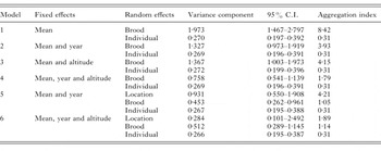
Table 1. Variance components of random effects in different models

Fig. 2. Goodness of model fit. Plots of residuals at the 3 different hierarchical levels of the random model with 2 fixed effects: estimated brood effects against standard Normal quantiles (A); estimated individual effects against standard Normal quantiles (B); and 3 realizations of the p–p plot for Poisson counts as described in the text (C) along with the 1:1 line expected under the Poisson model.
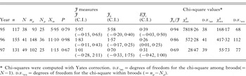
Table 2. Aggregation of sheep ticks on grouse chicks, within and among broods, according to the method of Boulinier et al. (1996)
 You have
Access
- 331
- Cited by