



1. Introduction
The study of random walks conditioned to stay positive (non-negative) has attracted significant research attention – see [Reference Bertoin and Doney4, Reference Biggins5, Reference Bolthausen7, Reference Caravenna9, Reference Iglehart21, Reference Tanaka26, Reference Vatutin and Wachtel27], to cite only a few. Recent progress has been made in more general cases: [Reference Denisov and Wachtel13] considered multidimensional random walks in general cones, [Reference Denisov, Sakhanenko and Wachtel12] treated the random walk with independent but non-identically distributed increments, and [Reference Grama, Lauvergnat and Le Page17] focused on Markov walks (which are time homogeneous). On the other hand, applications of random walks conditioned to stay positive appear in many situations. For example, the asymptotic behavior of the survival probability for critical branching processes in random environments is closely related to the behavior of the associated random walk conditioned to stay positive; see [Reference Afanasyev, Geiger, Kersting and Vatutin1, Reference Geiger and Kersting16, Reference Kozlov22]. The minimal position, additive martingale, and derivative martingale in branching random walks also make full use of some properties of random walks conditioned to stay positive; see [Reference Aïdékon2, Reference Aïdékon and Shi3, Reference Biggins and Kyprianou6, Reference Chen11, Reference Hu and Shi20].
The phrase ‘random walk conditioned to stay positive’ can be interpreted in two different ways. In the first interpretation, we can consider the random walk conditioned to stay positive up to time n, which can be viewed as a discrete version of the meander. The second interpretation involves conditioning on the event that the random walk never enters the interval
 $(\!-\infty,0)$
and can thus be regarded as a discrete version of the Bessel process, which is defined by Doob’s h-transform with the help of a harmonic function. In the latter case, it is a well-established fact that the renewal function associated with ladder height processes is harmonic for any oscillating random walk. This enables the definition of the random walk conditioned to stay positive via Doob’s h-transform. An essential tool for analyzing the asymptotic behavior of random walks conditioned to stay positive is the Wiener–Hopf factorization. For further details, please refer to the standard book, [Reference Feller15]. The aforementioned methods are fundamentally based on the duality principle, which asserts that if
 $\{S_n\}$
is a random walk then the distribution of the random path
 $\{S_k,k\leq n\}$
coincides with that of
 $\{S_n-S_{n-k},k\leq n\}$
.
Consider a model of random walk in a time-inhomogeneous random environment. An environment is given by a family of random variables
 $\xi=\{\xi_{n}\}$
, indexed by the time
 $n\in\mathbb{N}^*\,:\!=\,\{1,2,3,\ldots\}$
, defined on some probability space
 $(\Omega_{E},\mathcal{F}_{E},\mathrm{P})$
and taking values in the space of probability laws on
 $\mathbb{R}$
. In this paper, we assume that the environment
 $\{\xi_{n}\}_{n\in\mathbb{N}^*}$
is a sequence of stationary and ergodic random variables unless explicitly stated. Conditionally on
 $\xi$
, let
 $\{X_{n}\}_{n\in\mathbb{N}^*}$
be a sequence of independent real-valued random variables such that
 $X_n$
has probability law
 $\xi_n$
. Set
 $S_{0}\,:\!=\,x\in\mathbb{R}$
,
 $S_n\,:\!=\,S_0+\sum_{i=1}^{n}X_i$
,
 $n\geq1$
. The process
 $S=\{S_n\}$
thus constructed is a random walk with random environment in time starting from x (abbreviated as RWRE-t). We keep x fixed throughout the paper. In this model, it is observed that the environment is sampled randomly along the time axis. This is distinct from the scenario examined in the review notes in [Reference Zeitouni and Tavare28], wherein the environment is sampled randomly in space.
Let
 $(\Omega_\mathit{RW},\mathcal{F}_\mathit{RW},\mathbb{P}_{\xi})$
be the probability space under which the random walk is defined when the environment
 $\xi$
is fixed, and
 $\mathcal{F}^{\xi}_{n}\,:\!=\,\sigma(S_k, k\leq n)$
be the natural filtration of the process S. The total probability space can be formulated as the product space
 $(\Omega_{E}\times\Omega_\mathit{RW},\mathcal{F}_{E}\otimes\mathcal{F}_\mathit{RW},\mathbb{P})$
, where
 $\mathbb{P}\,:\!=\,\mathrm{P}\otimes \mathbb{P}_{\xi}$
in the sense that, for any non-negative measurable function f,
 \begin{align*}\int f\,\mathrm{d}\mathbb{P} =\int_{\Omega_{E}}\bigg(\int_{\Omega_\mathit{RW}}f(\xi,\omega)\,\mathrm{d}\mathbb{P}_{\xi}\bigg)\,\mathrm{d}\mathrm{P}.\end{align*}
Here, we call
 $\mathbb{P}_{\xi}$
the quenched probability and
 $\mathbb{P}$
the annealed probability. Note that the quenched probability is the conditional probability of
 $\mathbb{P}$
given the environment
 $\xi$
. The corresponding expectations with respect to
 $\mathbb{P}_{\xi}$
and
 $\mathbb{P}$
will be denoted by
 $\mathbb{E}_{\xi}$
and
 $\mathbb{E}$
, respectively.
The main objective of this paper is to construct random walks in a time-inhomogeneous random environment conditioned to stay positive. In addition to its intrinsic theoretical interest, a significant motivation to consider the RWRE-t conditioned to stay positive arises from the study of branching random walks with a random environment in time (BRWRE-t). As is usual practice, the celebrated many-to-one lemma can be employed to establish a relationship between BRWRE-t and RWRE-t. For example, [Reference Mallein and Miłoś23, Reference Mallein and Miłoś24] obtained the asymptotic behavior of the maximal position of BRWRE-t by investigating the ballot theorem for the associated RWRE-t. In our recent work [Reference Hong and Liang19], the quenched harmonic function and the construction of RWRE-t conditioned to stay positive play an essential role in proving the convergence of the derivative martingale for the BRWRE-t.
The difficulty lies in constructing a random walk in a time-inhomogeneous random environment conditioned to stay positive in the quenched sense. To this end, a key step is to formulate a (quenched) harmonic function. However, under the quenched probability,
 $\{S_n\}$
is a sum of independent but not necessarily identically distributed random variables and we lose the duality property. It is clear that the standard approach of defining the harmonic function by the underlying ladder process of the random walk is not possible, even if the random environment is independent and identically distributed. This raises the question of how we might define a harmonic function for RWRE-t.
In this paper, we establish a quenched function satisfying the harmonic property in a shift-invariance sense. This function is essentially dependent on the environment. In fact, inspired by the strong approximation method of [Reference Denisov, Sakhanenko and Wachtel12], we prove the existence of the limit of the overshoot
 $\lim_{n\to\infty}U_{n}(\xi,y)=U(\xi,y)\,:\!=\,-\mathbb{E}_\xi(S_{\tau_y})$
for almost every realization of
 $\xi$
, where
 $U_n(\xi,y)\,:\!=\,\mathbb{E}_\xi(y+S_n;\; \tau_{y}>n)$
and
 $\tau_{y}\,:\!=\,\inf\{n>0\colon y+S_n<0\}$
(see Theorem 1). It is demonstrated that the random function
 $U(\xi,y)$
is harmonic for the quenched random walk. Furthermore, some properties of the function
 $U(\xi,y)$
are derived (see Theorem 2 and Corollary 1). These constitute the primary contribution of the present paper.
With the quenched harmonic function in hand, we can construct the RWRE-t conditioned to stay positive, whose law is defined by Doob’s h-transform: for any
 $n\geq1$
and
 $B\in\mathcal{F}^{\xi}_n$
,
 \begin{equation*} \mathbb{P}^+_{\xi}(B) \,:\!=\, \frac{\mathbb{E}_{\xi}(U(\theta^n\xi, S_n)\mathbf{1}_{\{\tau_0>n\}}\mathbf{1}_B)}{U(\xi,0)}.\end{equation*}
The terminology conditioned to stay positive can be justified by the following result (see Theorem 3):
 $\mathbb{P}^+_{\xi}(\cdot)=\lim_{n\to\infty}\mathbb{P}_{\xi}(\cdot\mid S_0\geq 0,S_1\geq 0,\ldots,S_n\geq 0)$
.
The rest of this paper is organized as follows. In Section 2, we present our main results on the existence and preliminary properties of a quenched harmonic function for the RWRE-t, and we construct random walks conditioned to stay positive for almost all
 $\xi$
. The proofs of the main results are provided in Section 3.
2. Main results
2.1. Quenched harmonic function
In this subsection, we identify a quenched harmonic function for the RWRE-t. The earlier approach to formulating the harmonic function by means of the underlying ladder process of random walks is not applicable in this case. For this purpose, the shifted environment is employed to define a quenched harmonic function based on two steps.
Firstly, let
 $y\geq0$
, denote by
 $\tau_{y}$
the first moment when
 $\{S_n\}$
enters the interval
 $(\!-\infty, -y)$
:
 $\tau_{y}\,:\!=\,\inf\{n>0\colon y+S_n<0\}$
. Define
 $U_n(\xi,y)\,:\!=\,\mathbb{E}_\xi(y+S_n;\;\tau_{y}>n)$
. Let
 $\theta$
be the shift operator, i.e.
 $\theta\xi\,:\!=\,(\xi_2,\xi_3,\ldots)$
. For
 $n\geq1$
,
 $\theta^n\xi\,:\!=\,\theta(\theta^{n-1}\xi)$
with the convention that
 $\theta^0\xi\,:\!=\,\xi$
.
Drawing inspiration from the universality approach employed in [Reference Denisov, Sakhanenko and Wachtel12], the existence of the limit
 $\lim_{n\to\infty}U_{n}(\xi,y)=U(\xi,y)\,:\!=\,-\mathbb{E}_\xi(S_{\tau_y})$
for almost every realization of
 $\xi$
is established in the following theorem. To get rid of the trivial case, we assume throughout this paper that
 $\mathbb{P}_\xi(X_1>0)>0$
P-almost surely (a.s.).
Theorem 1. Assume that
 \begin{equation} \mathbb{E}_\xi(X_1)=0 \quad \mathrm{P}{-a.s.}, \qquad \mathbb{E}|X_1|^{2+\varepsilon}<\infty \quad \textit{for some}\ \varepsilon>0. \end{equation}
Then there exists a random variable
 $U(\xi,y)$
such that, for almost all
 $\xi$
,
 \begin{align*}\lim\limits_{n\to\infty}U_{n}(\xi,y)=U(\xi,y)\,:\!=\,-\mathbb{E}_\xi(S_{\tau_y}).\end{align*}
Remark 1. Regarding the second condition in (1), the exponent
 $\varepsilon$
is not strictly essential. By carefully examining the proof of Lemma 5, we can relax the moment assumption to
 \begin{align*}\mathbb{E}[X_1^2\log^{2+\varepsilon}(1+|X_1|)] < \infty \quad \text{for some}\ \varepsilon>0.\end{align*}
Secondly, note that the limiting function
 $U(\xi,\cdot)$
is random and measurable with respect to
 $\sigma(\xi)\,:\!=\,\sigma(\xi_{1},\xi_2,\ldots)$
. By shifting the environment, we obtain a family
 $\{U(\theta^n\xi,\cdot)\}$
of functions. Based on the observation that the function
 $U(\xi,\cdot)$
is shift invariant for the semigroup of the random walk killed when it first enters
 $(\!-\infty,0)$
in the quenched sense, we will prove that
 $U(\xi,\cdot)$
can serve as a positive quenched harmonic function that plays an essential role in defining the quenched random walk conditioned to stay positive. The ‘usual’ properties of the harmonic function are also established.
Theorem 2. Assume that (1) holds, and
 $U(\xi,y)$
is defined as in Theorem 1. Then:
-
(i) U is
 $\sigma(\xi)$
-measurable and satisfies the quenched harmonic property:
\begin{align*}U(\xi,y)=\mathbb{E}_{\xi}[U(\theta\xi,y+S_{1});\;\tau_{y}>1] \quad \mathrm{P}{-a.s.}\end{align*}
-
(ii)
$U(\xi,y)$
is positive, non-decreasing in y, and (2)
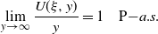
\begin{equation} \lim\limits_{y\to\infty}\frac{U(\xi,y)}{y}=1 \quad \mathrm{P}{-a.s.} \end{equation}



Corollary 1. Under the assumption of Theorem 2, for almost all
 $\xi$
we have:
-
(i)
$\{U(\theta^n\xi,y+S_n)\mathbf{1}_{\{\tau_{y}>n\}}\}_{n\in\mathbb{N}^*}$
is a martingale with respect to the filtration
$(\mathcal{F}^{\xi}_{n})$
under
$\mathbb{P}_\xi$
. -
(ii) For any
$y_n\geq0$
with
$y_n\to \infty$
as
$n\to \infty$
,
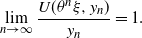
\begin{equation*} \lim\limits_{n\to\infty}\frac{U(\theta^n\xi,y_n)}{y_n}=1. \end{equation*}
-
(iii) The quenched probability of the random walk to stay positive is given by
(3)where
\begin{equation} \mathbb{P}_\xi(\tau_y>n) \sim \frac{\sqrt{2}U(\xi,y)}{\sqrt{\pi n}\sigma} \quad {as}\ n\to\infty, \end{equation}
$\sigma^2\,:\!=\,\mathbb{E}(X^2_1)$
.





Remark 2. The quenched harmonic function is a new and useful tool to study an RWRE-t conditioned to stay positive in the quenched probability. It is worth noting that
 $U(\xi,y)$
depends on the whole sequence
 $\xi=\{\xi_{n}\}_{n\in\mathbb{N}^*}$
of random variables. Although
 $\{U(\theta^n\xi,y+S_n)\mathbf{1}_{\{\tau_{y}>n\}}\}_{n\in\mathbb{N}^*}$
is a martingale with respect to the filtration
 $(\mathcal{F}^{\xi}_{n})$
under
 $\mathbb{P}_\xi$
, it is not a martingale with respect to the filtration
 $(\sigma(\xi_1,\ldots,\xi_n)\otimes\mathcal{F}^{\xi}_{n})$
under the annealed law
 $\mathbb{P}$
. The quenched harmonic function
 $U(\xi,y)$
cannot be obtained in the annealed probability
 $\mathbb{P}$
even for the independent and identically distributed random environment.
2.2. Random walk conditioned to stay positive
In this subsection, we introduce a random walk conditioned to stay positive for almost all
 $\xi$
using the quenched harmonic function
 $U(\xi,y)$
. It is assumed that (1) remains valid throughout this discussion.
By Corollary 1(i), for any
 $n\geq1$
,
 $y\geq0$
, and
 $B\in\mathcal{F}^{\xi}_n$
, we can define the law of this conditioned walk by Doob’s h-transform:
 \begin{equation} \mathbb{P}^+_{\xi,y}(B) \,:\!=\, \frac{\mathbb{E}_{\xi,y}(U(\theta^n\xi,S_n)\mathbf{1}_{\{\tau_0>n\}}\mathbf{1}_B)}{U(\xi,y)}.\end{equation}
The process
 $\{S_n\}$
under the probability
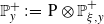 $\mathbb{P}^+_y\,:\!=\,\mathrm{P}\otimes\mathbb{P}^+_{\xi,y}$
is called a random walk in a time random environment, started at y, conditioned to stay positive. We omit the subscript in the case where
 $y=0$
. Indeed, given the environment
 $\xi$
, it is a Markov chain with state space
 $[0,\infty)$
and the transition kernel given by
 \begin{align*}\mathbb{P}^{+}_{\xi}(x;\;\mathrm{d}y) \,:\!=\,\frac{U(\theta\xi,y)\mathbf{1}_{\{y\geq0\}}}{U(\xi,x)}\mathbb{P}_{\xi,x}(S_{1}\in\mathrm{d}y).\end{align*}
The following result shows that the probability measure
 $\mathbb{P}^+_{\xi}$
arises from conditioning on the event that the random walk stays positive up to time n:
 $\mathbb{P}_{\xi}(\cdot\mid\tau_{0}>n)$
.
Theorem 3. For
 $k\in\mathbb{N}^*$
, let
 $f(S)=f(S_0,S_1,\ldots,S_k)$
be a bounded functional that depends only on the first k steps of S. Then, for almost all
 $\xi$
,
 $\lim_{n\to\infty}\mathbb{E}_{\xi}(f(S)\mid\tau_0>n) = \mathbb{E}^+_{\xi}(f(S))$
.
Remark 3. This result was established in [Reference Bertoin and Doney4] in the context of a random walk with a constant environment. Many authors have also studied the invariance principles for random walks conditioned to stay positive; see, for example, [Reference Bolthausen7, Reference Bryn-Jones and Doney8, Reference Caravenna and Chaumont10, Reference Doney14, Reference Iglehart21]. For the case in a random environment, we refer to [Reference Hong and Liang18].
Remark 4. To investigate the behavior of a random walk conditioned to stay positive, Tanaka’s decomposition is an invaluable tool; see, e.g., [Reference Afanasyev, Geiger, Kersting and Vatutin1, Reference Biggins5, Reference Tanaka26]. It is important to note that it is not possible to reconstruct the random walk conditioned to stay positive by the independent and identically distributed excursions of a reversed ladder process, as is the case with the usual random walk, due to the time inhomogeneity and the dependency on
 $\xi$
of our harmonic function. The absence of homogeneity makes the management of this process difficult and also gives rise to new phenomena. A version of Tanaka’s decomposition for our conditioned random walk and its application are given in [Reference Hong and Liang19, Section 2].
3. Proofs
3.1. Proof of Theorem 1
In this subsection, we adapt the approach in [Reference Denisov, Sakhanenko and Wachtel12] to show that the function
 $U(\xi,\cdot)$
is well defined for almost all
 $\xi$
. A key step is to prove that the random variable
 $S_{\tau_{y}}$
is integrable under
 $\mathbb{P}_{\xi}$
for almost all
 $\xi$
(see Lemma 5).
First, we give the fact that
 $\mathbb{P}_{\xi}(\tau_{y}<\infty)=1$
for almost all
 $\xi$
(Lemma 2). This is achieved through the strong approximation method, which is based on the implicit rate of convergence in the invariance principle.
Lemma 1. Given the environment
 $\xi$
, for every
 $n\geq1$
we can reconstruct a random walk
 $\{S_n\}_{n\in\mathbb{N}^*}$
and a standard Brownian motion
 $\{W^n_t\}_{t\in\mathbb{R}_+}$
on a common probability space such that
 $\mathbb{P}_{\xi}\big(\sup_{0\leq t\leq1}|S_{(nt)}-W^n_{n\sigma^2 t}| > \sqrt{n}\sigma\pi_{n}\big) \leq \pi_{n}$
, where
 $\sigma^2\,:\!=\,\mathbb{E}(X^2_1)$
,
 $\pi_{n}$
(depending on
 $\xi$
) denotes the Prokhorov distance between the distribution on C[0,1] of the process
 $S_{(\cdot)}$
(the linear interpolation of S) and the Brownian motion
 $W^n_{\cdot}$
, and, for almost every realization of
 $\xi$
,
 $\pi_{n}\to0$
as
 $n\to\infty$
.
Proof. This result is a consequence of [Reference Denisov, Sakhanenko and Wachtel12, Lemma 16] and [Reference Sakhanenko25, Remark 2]. Note that
 $\sum_{i=1}^n\mathbb{E}_{\xi}(X_i^2)\sim n\sigma^2$
P-a.s. as
 $n\to\infty$
, and assumption (1) implies that, for almost every realization of
 $\xi$
, the Lindeberg condition holds, which is equivalent to the Prokhorov distance
 $\pi_{n}$
tending to 0.
Lemma 2. For almost all
 $\xi$
,
 $\tau_{y}<\infty$
 $\mathbb{P}_\xi$
-a.s.
Proof. Note that since
 $\big|\inf_{t\leq 1}S_{(nt)}-\inf_{t\leq 1}W^n_{n\sigma^2 t}\big|\leq\sup_{t\leq 1}\big|S_{(nt)}-W^n_{n\sigma^2 t}\big|$
, we have
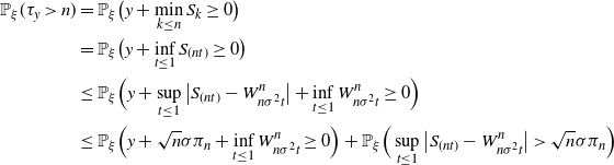 \begin{align*} \mathbb{P}_{\xi}(\tau_{y}>n) & = \mathbb{P}_{\xi}\big(y+\min_{k\leq n}S_{k}\geq0\big) \\ & = \mathbb{P}_{\xi}\big(y+\inf_{t\leq 1}S_{(nt)}\geq0\big) \\ & \leq \mathbb{P}_{\xi}\Big(y+\sup_{t\leq1}\big|S_{(nt)}-W^n_{n\sigma^2t}\big|+\inf_{t\leq1}W^n_{n\sigma^2t}\geq0\Big) \\ & \leq \mathbb{P}_{\xi}\Big(y+\sqrt{n}\sigma\pi_{n}+\inf_{t\leq1}W^n_{n\sigma^2t}\geq0\Big) + \mathbb{P}_{\xi}\Big(\sup_{t\leq1}\big|S_{(nt)}-W^n_{n\sigma^2t}\big|>\sqrt{n}\sigma\pi_{n}\Big) \end{align*}
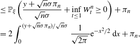 \begin{align*} & \leq \mathbb{P}_{\xi}\bigg(\frac{y+\sqrt{n}\sigma\pi_{n}}{\sqrt{n}\sigma} + \inf_{t\leq 1}W^n_{t}\geq0\bigg) + \pi_{n} \\ & = 2\int_{0}^{({y+\sqrt{n}\sigma\pi_{n}})/{\sqrt{n}\sigma}}\frac{1}{\sqrt{2\pi}\,}\mathrm{e}^{-{x^2}/{2}}\,\mathrm{d}x + \pi_{n}, \end{align*}
where the last inequality follows by Lemma 1. Since, for almost every realization of
 $\xi$
,
 $\pi_{n}\to0$
as
 $n\to\infty$
, it follows that
 $\mathbb{P}_{\xi}(\tau_{y}>n)\to0$
.
Next, we prove the integrability of
 $S_{\tau_{y}}$
under
 $\mathbb{P}_{\xi}$
for almost all
 $\xi$
. We begin by giving an upper bound for
 $\mathbb{P}_{\xi}(\tau_{y}>n)$
.
Lemma 3. Fix
 $y\geq0$
. For almost all
 $\xi$
, there exists an integer
 $N_1$
(depending on
 $\xi$
and y) such that, for all
 $n>N_1$
,
 $\mathbb{P}_{\xi}(\tau_{y}>n)<{3U_n(\xi,y)}/{\sqrt{n}\sigma}$
.
Proof. For any
 $n\geq1$
,
 $x\in\mathbb{R}$
, we have
 $\mathbb{P}_{\xi}(S_n>x,\tau_{y}>n)\geq\mathbb{P}_{\xi}(S_n>x)\mathbb{P}_{\xi}(\tau_{y}>n)$
, which is a direct consequence of the Fortuin–Kasteleyn–Ginibre inequality. Hence, we get
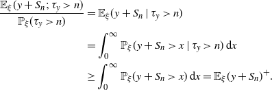 \begin{align*} \begin{aligned} \frac{\mathbb{E}_{\xi}(y+S_n;\;\tau_{y}>n)}{\mathbb{P}_{\xi}(\tau_{y}>n)} & = \mathbb{E}_{\xi}(y+S_n\mid\tau_{y}>n) \\ & = \int_{0}^{\infty}\mathbb{P}_{\xi}(y+S_n>x\mid\tau_{y}>n)\,\mathrm{d}x \\ & \geq \int_{0}^{\infty}\mathbb{P}_{\xi}(y+S_n>x)\,\mathrm{d}x = \mathbb{E}_{\xi}(y+S_n)^+. \end{aligned} \end{align*}
On the other hand, by the central limit theorem, for almost all
 $\xi$
,
 $({y+S_n})/{\sqrt{n}\sigma}$
converges in law (
 $\mathbb{P}_{\xi}$
) to the standard normal distribution. By Fatou’s lemma, we obtain
 \begin{align*} \liminf_{n\to\infty}\frac{\mathbb{E}_{\xi}(y+S_n)^+}{\sqrt{n}\sigma} \geq \int_{0}^{\infty}\frac{x}{\sqrt{2\pi}\,}\mathrm{e}^{-{x^2}/{2}}\,\mathrm{d}x = \frac{1}{\sqrt{2\pi}\,} > \frac{1}{3}, \end{align*}
so we can choose
 $N_1\,:\!=\,\max\{n\geq1\colon\mathbb{E}_{\xi}(y+S_n)^+\leq{\sqrt{n}\sigma}/{3}\}<\infty$
.
Therefore, for all
 $n>N_1$
,
 \begin{align*} \mathbb{P}_{\xi}(\tau_{y}>n) \leq \frac{\mathbb{E}_\xi(y+S_n;\;\tau_{y}>n)}{\mathbb{E}_{\xi}(y+S_n)^+} \leq \frac{3\mathbb{E}_\xi(y+S_n;\;\tau_{y}>n)}{\sqrt{n}\sigma} \end{align*}
yields the desired result.
For simplicity, let us introduce some more notation:
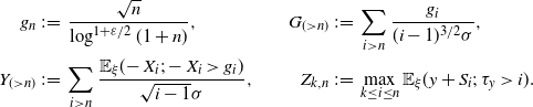 \begin{alignat*}{2} g_n & \,:\!=\, \frac{\sqrt{n}}{\log^{1+{\varepsilon}/{2}}(1+n)}, & G_{(>n)} & \,:\!=\, \sum_{i>n}\frac{g_i}{(i-1)^{{3}/{2}}\sigma}, \\ Y_{(>n)} & \,:\!=\, \sum_{i>n}\frac{\mathbb{E}_{\xi}(\!-X_i;-X_i>g_i)}{\sqrt{i-1}\sigma}, \qquad & Z_{k,n} & \,:\!=\, \max_{k\leq i\leq n}\mathbb{E}_{\xi}(y+S_i;\;\tau_{y}>i).\end{alignat*}
Lemma 4. Fix
 $y\geq0$
, and let
 $N_1$
be the same as in Lemma 3. Then, for almost all
 $\xi$
, for
 $N_1\leq N_2\leq k\leq n$
we have
 \begin{align} \mathbb{E}_{\xi}(g_{\tau_{y}},N_2<\tau_{y}\leq k) & \leq 3Z_{N_2,n}G_{(>N_2)},\end{align}
 \begin{align} \mathbb{E}_{\xi}(\!-X_{\tau_{y}};-X_{\tau_{y}}>g_{\tau_{y}},N_2<\tau_{y}\leq k) & \leq 3Z_{N_2,n}Y_{(>N_2)}. \end{align}
Proof. To prove (5), note that
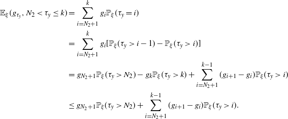 \begin{align*} \mathbb{E}_{\xi}(g_{\tau_{y}},N_2<\tau_{y}\leq k) & = \sum_{i=N_{2}+1}^{k}g_{i}\mathbb{P}_{\xi}(\tau_{y}=i) \\ & = \sum_{i=N_{2}+1}^{k}g_{i}[\mathbb{P}_{\xi}(\tau_{y}>i-1)-\mathbb{P}_{\xi}(\tau_{y}>i)] \\ & = g_{N_2+1}\mathbb{P}_{\xi}(\tau_{y}>N_2) - g_k\mathbb{P}_{\xi}(\tau_{y}>k) + \sum_{i=N_{2}+1}^{k-1}(g_{i+1}-g_i)\mathbb{P}_{\xi}(\tau_{y}>i) \\ & \leq g_{N_2+1}\mathbb{P}_{\xi}(\tau_{y}>N_2) + \sum_{i=N_{2}+1}^{k-1}(g_{i+1}-g_i)\mathbb{P}_{\xi}(\tau_{y}>i). \end{align*}
Then, by applying Lemma 3 and the definitions of
 $Z_{k,n}$
and
 $G_{(>n)}$
, we obtain
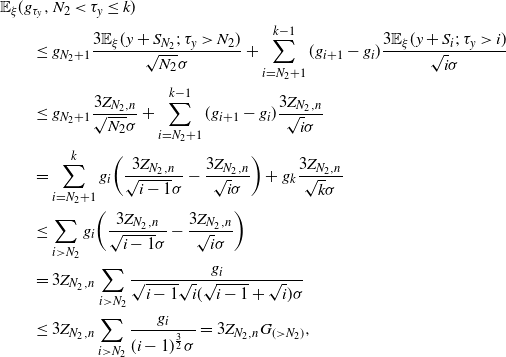 \begin{align*} & \mathbb{E}_{\xi}(g_{\tau_{y}},N_2<\tau_{y}\leq k) \\ & \qquad \leq g_{N_2+1}\frac{3\mathbb{E}_{\xi}(y+S_{N_2};\,\tau_{y}>N_2)}{\sqrt{N_2}\sigma} + \sum_{i=N_{2}+1}^{k-1}(g_{i+1}-g_i)\frac{3\mathbb{E}_{\xi}(y+S_i;\;\tau_{y}>i)}{\sqrt{i}\sigma} \\ & \qquad \leq g_{N_2+1}\frac{3Z_{N_2,n}}{\sqrt{N_2}\sigma} + \sum_{i=N_{2}+1}^{k-1}(g_{i+1}-g_i)\frac{3Z_{N_2,n}}{\sqrt{i}\sigma} \\ & \qquad = \sum_{i=N_{2}+1}^{k}g_i\bigg(\frac{3Z_{N_2,n}}{\sqrt{i-1}\sigma}-\frac{3Z_{N_2,n}}{\sqrt{i}\sigma}\bigg) + g_{k}\frac{3Z_{N_2,n}}{\sqrt{k}\sigma} \\ & \qquad \leq \sum_{i>N_{2}}g_i\bigg(\frac{3Z_{N_2,n}}{\sqrt{i-1}\sigma}-\frac{3Z_{N_2,n}}{\sqrt{i}\sigma}\bigg) \\ & \qquad = 3Z_{N_2,n}\sum_{i>N_{2}}\frac{g_i}{\sqrt{i-1}\sqrt{i}(\sqrt{i-1}+\sqrt{i})\sigma} \\ & \qquad \leq 3Z_{N_2,n}\sum_{i>N_{2}}\frac{g_i}{(i-1)^{\frac{3}{2}}\sigma} = 3Z_{N_2,n}G_{(>N_2)}, \end{align*}
where the second to last inequality holds since
 $g_n$
is positive and increasing in n.
To prove (6), observe that
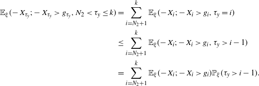 \begin{align*} \mathbb{E}_{\xi}(\!-X_{\tau_{y}};-X_{\tau_{y}}>g_{\tau_{y}},N_2<\tau_{y}\leq k) & = \sum_{i=N_{2}+1}^{k}\mathbb{E}_{\xi}(\!-X_{i};-X_{i}>g_{i},\tau_{y}=i) \\ & \leq \sum_{i=N_{2}+1}^{k}\mathbb{E}_{\xi}(\!-X_{i};-X_{i}>g_{i},\tau_{y}>i-1) \\ & = \sum_{i=N_{2}+1}^{k}\mathbb{E}_{\xi}(\!-X_{i};-X_{i}>g_{i})\mathbb{P}_{\xi}(\tau_{y}>i-1). \end{align*}
Again using Lemma 3 and the definitions of
 $Z_{k,n}$
and
 $Y_{(>n)}$
, we get
 \begin{align*} \mathbb{E}_{\xi}(\!-X_{\tau_{y}};-X_{\tau_{y}}>g_{\tau_{y}},N_2<\tau_{y}\leq k) & \leq \sum_{i=N_{2}+1}^{k}\mathbb{E}_{\xi}(\!-X_{i};-X_{i}>g_{i}) \frac{3\mathbb{E}_{\xi}(y+S_{i-1};\;\tau_{y}>i-1)}{\sqrt{i-1}\sigma} \\ & \leq 3Z_{N_2,n}\sum_{i>N_{2}}\frac{\mathbb{E}_{\xi}(\!-X_{i};-X_{i}>g_{i})}{\sqrt{i-1}\sigma} = 3Z_{N_2,n}Y_{(>N_2)}. \end{align*}
Lemma 5. For any
 $y\geq0$
,
 $\mathbb{E}_\xi |S_{\tau_{y}}|<\infty\; \mathrm{P}$
-a.s.
Proof. First, note that since
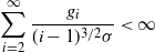 \begin{align*}\sum_{i=2}^{\infty}\frac{g_i}{(i-1)^{{3}/{2}}\sigma}<\infty\end{align*}
we get
 $G_{(>n)}\to0$
as
 $n\to\infty$
, and (1) implies that, for almost all
 $\xi$
,
 $Y_{(>n)}\to0$
as
 $n\to\infty$
. In fact, using (1) and Markov’s inequality, we have
 $\mathbb{P}(\!-X_1>g_i)\leq {C_0}/{g_i^{2+\varepsilon}}$
, where
 $C_0\,:\!=\,\mathbb{E}|X_1|^{2+\varepsilon}<\infty$
. Integrating by parts yields
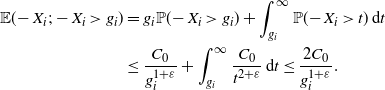 \begin{align*} \mathbb{E}(\!-X_i;-X_i>g_i) & = g_i\mathbb{P}(\!-X_i>g_i) + \int_{g_i}^{\infty}\mathbb{P}(\!-X_i>t)\,\mathrm{d}t \\ & \leq \frac{C_0}{g_i^{1+\varepsilon}} + \int_{g_i}^{\infty}\frac{C_0}{t^{2+\varepsilon}}\,\mathrm{d}t \leq \frac{2C_0}{g_i^{1+\varepsilon}}. \end{align*}
Thus, recalling the definition of
 $g_i$
, we have
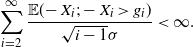 \begin{align*}\sum_{i=2}^{\infty}\frac{\mathbb{E}(\!-X_i;-X_i>g_i)}{\sqrt{i-1}\sigma}<\infty.\end{align*}
This implies that, for almost all
 $\xi$
,
 $Y_{(>n)}\to0$
as
 $n\to\infty$
. As a result, for almost all
 $\xi$
we can choose
 $N_2\,:\!=\,\min\big\{n>N_1\colon G_{(>n)}+Y_{(>n)}\leq\frac{1}{6}\big\}<\infty$
.
Next, since
 $y+S_{i-1}\geq0$
in the event
 $\{\tau_{y}=i\}$
, we get
 \begin{align*} -y-S_{\tau_{y}} = -y-S_{\tau_{y}-1}-X_{\tau_{y}} \leq -X_{\tau_{y}} \leq g_{\tau_{y}} - X_{\tau_{y}}\mathbf{1}_{\{-X_{\tau_{y}}>g_{\tau_{y}}\}}. \end{align*}
From this inequality and Lemma 4, for
 $N_2\leq k\leq n$
we obtain
 \begin{align*} & \mathbb{E}_{\xi}(\!-y-S_{\tau_{y}};\;\tau_{y}\leq k) \\ & \quad \leq \mathbb{E}_{\xi}(\!-y-S_{\tau_{y}};\;\tau_{y}\leq N_2) + \mathbb{E}_{\xi}(g_{\tau_{y}};\;N_2<\tau_{y}\leq k) + \mathbb{E}_{\xi}(\!-X_{\tau_{y}};-X_{\tau_{y}}>g_{\tau_{y}},N_2<\tau_{y}\leq k) \\ & \quad \leq C_1 + 3Z_{N_2,n}G_{(>N_2)} + 3Z_{N_2,n}Y_{(>N_2)} \leq C_1 + {Z_{N_2,n}}/{2}, \end{align*}
where
 $C_1\,:\!=\,\mathbb{E}_{\xi}(\!-y-S_{\tau_{y}};\;\tau_{y}\leq N_2)$
. Note that
 $C_1$
depends on
 $\xi$
and
 $C_1<\infty$
for almost all
 $\xi$
. In fact,
 \begin{align*} \mathbb{E}_{\xi}(\!-y-S_{\tau_{y}};\;\tau_{y}\leq N_2) = \sum_{i=1}^{N_2}\mathbb{E}_{\xi}(\!-y-S_{i};\;\tau_{y}=i) \leq \sum_{i=1}^{N_2}\mathbb{E}_{\xi}((y+S_{i})^{-}) < \infty. \end{align*}
Then, by the optional stopping theorem (see (7)), for
 $N_2\leq k\leq n$
we get
 \begin{align*}\mathbb{E}_\xi(y+S_{k};\;\tau_{y}>k) = y +\mathbb{E}_\xi(\!-y-S_{\tau_{y}};\;\tau_{y}\leq k) \leq y + C_1 + {Z_{N_2,n}}/{2}.\end{align*}
Taking the maximum in the last inequality with respect to
 $k\in[N_2,n]$
, we get
 $Z_{N_2,n} \leq y+C_1+{Z_{N_2,n}}/{2}$
, which implies that
 $Z_{N_2,n}\leq 2y+2C_1$
.
Therefore,
 $\mathbb{E}_{\xi}(\!-y-S_{\tau_{y}};\;\tau_{y}\leq n)\leq y+2C_1$
. By the monotone convergence theorem, we have
 $0\leq\mathbb{E}_{\xi}(\!-y-S_{\tau_{y}})=\lim_{n\to\infty}\mathbb{E}_{\xi}(\!-y-S_{\tau_{y}};\;\tau_{y}\leq n)\leq y+2C_1$
, which implies that
 $0\leq-\mathbb{E}_{\xi}(S_{\tau_{y}})\leq 2y+2C_1$
.
Proof of Theorem
1. Since
 $\{S_n\}$
is a martingale under
 $\mathbb{P}_\xi$
, for any
 $n\geq1$
, by the optional stopping theorem, we have
 $0=\mathbb{E}_\xi(S_{n\wedge\tau_{y}})=\mathbb{E}_\xi(S_{\tau_{y}};\;\tau_{y}\leq n)+\mathbb{E}_\xi(S_{n};\;\tau_{y}>n)$
. That is,
 $\mathbb{E}_\xi(S_{n};$
 $\tau_{y}>n)=-\mathbb{E}_\xi(S_{\tau_{y}};\;\tau_{y}\leq n)$
. Then
 \begin{equation} \mathbb{E}_\xi(y+S_{n};\;\tau_{y}>n)=y\mathbb{P}_\xi(\tau_{y}>n)-\mathbb{E}_\xi(S_{\tau_{y}};\;\tau_{y}\leq n). \end{equation}
By Lemmas 2 and 5 and the dominated convergence theorem,
 \begin{align*}\lim_{n\to\infty}U_n(\xi,y)=\lim_{n\to\infty}\mathbb{E}_\xi(y+S_{n};\;\tau_{y}>n)=-\mathbb{E}_\xi(S_{\tau_{y}}).\end{align*}
Theorem 1 follows.
3.2. Proof of Theorem 2
The idea for the proof of the quenched harmonic property is simple: express
 $U_{n+1}(\xi,y)$
as the integral of
 $U_{n}(\theta\xi,y')$
by the Markov property, then the quenched harmonic property follows by the dominated convergence theorem. Our idea is based on the fact that the random environment is an infinite sequence of random elements. By shifting the environment, we obtain the quenched harmonic property rather than the annealed harmonic property.
Proof of Theorem
2(i). By the Markov property, and under
 $\mathbb{P}_{\theta\xi}$
, the random walk is
 $S_{n}=\sum_{i=2}^{n+1}X_{i}$
. We obtain, for
 $n\geq1$
,
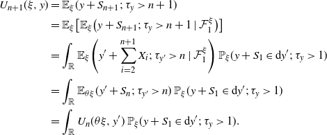 \begin{align} U_{n+1}(\xi,y) & = \mathbb{E}_\xi(y+S_{n+1};\; \tau_{y}>n+1) \nonumber \\ & = \mathbb{E}_\xi\big[\mathbb{E}_\xi\big(y+S_{n+1};\; \tau_{y}>n+1\mid \mathcal{F}^{\xi}_{1}\big)\big] \nonumber \\ & = \int_{\mathbb{R}}\mathbb{E}_\xi\Bigg(y'+\sum_{i=2}^{n+1}X_{i};\;\tau_{y'}>n\mid\mathcal{F}^{\xi}_{1}\Bigg)\, \mathbb{P}_\xi(y+S_1\in\mathrm{d}y';\;\tau_{y}>1) \nonumber \\ & = \int_{\mathbb{R}}\mathbb{E}_{\theta\xi}(y'+S_{n};\;\tau_{y'}>n)\,\mathbb{P}_\xi(y+S_1\in\mathrm{d}y';\;\tau_{y}>1) \nonumber \\ & = \int_{\mathbb{R}}U_n(\theta\xi,y')\,\mathbb{P}_\xi(y+S_1\in\mathrm{d}y';\;\tau_{y}>1). \end{align}
Note that
 $U_{n}(\xi,y)$
is non-decreasing in n, since the sequence
 $\{(y+S_n)\mathbf{1}_{\{\tau_{y}>n\}}\}$
is a submartingale. In fact, we have
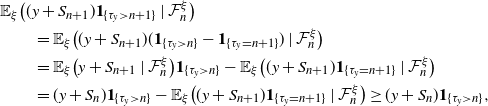 \begin{align*} & \mathbb{E}_{\xi}\big((y+S_{n+1})\mathbf{1}_{\{\tau_{y}>n+1\}}\mid\mathcal{F}^{\xi}_{n}\big) \\ & \qquad = \mathbb{E}_{\xi}\big((y+S_{n+1})(\mathbf{1}_{\{\tau_{y}>n\}}-\mathbf{1}_{\{\tau_{y}=n+1\}}) \mid \mathcal{F}^{\xi}_{n}\big) \\ & \qquad = \mathbb{E}_{\xi}\big(y+S_{n+1}\mid\mathcal{F}^{\xi}_{n}\big)\mathbf{1}_{\{\tau_{y}>n\}} - \mathbb{E}_{\xi}\big((y+S_{n+1})\mathbf{1}_{\{\tau_{y}=n+1\}}\mid\mathcal{F}^{\xi}_{n}\big) \\ & \qquad = (y+S_{n})\mathbf{1}_{\{\tau_{y}>n\}} - \mathbb{E}_{\xi}\big((y+S_{n+1})\mathbf{1}_{\{\tau_{y}=n+1\}}\mid\mathcal{F}^{\xi}_{n}\big) \geq (y+S_{n})\mathbf{1}_{\{\tau_{y}>n\}}, \end{align*}
where the last inequality follows from the fact that
 $y+S_{n+1}<0$
on the event
 $\{\tau_{y}=n+1\}$
. This yields the submartingale property.
Taking the limit in (8), by Lemma 5 and the dominated convergence theorem we get
 \begin{equation*} U(\xi,y) = \int_{\mathbb{R}}U(\theta\xi,y')\,\mathbb{P}_\xi(y+S_1\in\mathrm{d}y';\; \tau_{y}>1) = \mathbb{E}_{\xi}[U(\theta \xi,y+S_{1});\;\tau_{y}>1], \end{equation*}
and claim (i) follows.
To obtain the asymptotic behavior of the quenched harmonic function, we construct a non-negative supermartingale in the following lemma.
Lemma 6. For
 $C\in\mathbb{R}_{+}$
and
 $K\in\mathbb{N}^*$
, let
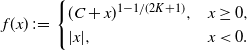 \begin{equation*} f(x) \,:\!=\, \begin{cases} (C+x)^{1-{1}/({2K+1})}, & x\geq0, \\ |x|, & x<0. \end{cases} \end{equation*}
Then, for almost all
 $\xi$
, there exist sufficiently large C and K (both depending on
 $\xi$
) such that
 $f(y+S_{n\wedge\tau_y})$
is a non-negative supermartingale under
 $\mathbb{P}_\xi$
.
Proof. Fix each realization of
 $\xi$
. We first show the integrability of
 $f(y+S_{n\wedge\tau_y})$
under
 $\mathbb{P}_\xi$
. For each n, we have
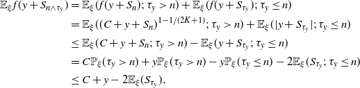 \begin{align*} \mathbb{E}_{\xi}f(y+S_{n\wedge\tau_y}) & = \mathbb{E}_{\xi}(f(y+S_{n});\;\tau_{y}>n) + \mathbb{E}_{\xi}(f(y+S_{\tau_y});\;\tau_{y}\leq n) \\ & = \mathbb{E}_{\xi}((C+y+S_{n})^{1-{1}/({2K+1})};\;\tau_{y}>n) + \mathbb{E}_{\xi}(|y+S_{\tau_y}|;\;\tau_{y}\leq n) \\ & \leq \mathbb{E}_{\xi}(C+y+S_{n};\;\tau_{y}>n) - \mathbb{E}_{\xi}(y+S_{\tau_y};\;\tau_{y}\leq n) \\ & = C\mathbb{P}_{\xi}(\tau_{y}>n) + y\mathbb{P}_{\xi}(\tau_{y}>n) - y\mathbb{P}_{\xi}(\tau_{y}\leq n) - 2\mathbb{E}_{\xi}(S_{\tau_y};\;\tau_{y}\leq n) \\ & \leq C+y-2\mathbb{E}_{\xi}(S_{\tau_{y}}), \end{align*}
where the last equality follows from
 $\mathbb{E}_\xi(S_{n};\;\tau_{y}>n)=-\mathbb{E}_\xi(S_{\tau_{y}};\;\tau_{y}\leq n)$
. Therefore, by Lemma 5, we obtain that, for almost all
 $\xi$
,
 $\mathbb{E}_{\xi}f(y+S_{n\wedge\tau_y})<\infty$
.
Next, we prove the supermartingale property, i.e.
 \begin{align} \mathbb{E}_{\xi}\big[f(y+S_{(n+1)\wedge\tau_y})\mid\mathcal{F}^{\xi}_{n}\big] & \leq f(y+S_{n\wedge\tau_y}) \nonumber \\ & = (C+y+S_{n})^{1-{1}/({2K+1})}\mathbf{1}_{\{\tau_{y}>n\}} + |y+S_{\tau_y}|\mathbf{1}_{\{\tau_{y}\leq n\}}. \end{align}
By the definitions of
 $\tau_{y}$
and f(x), we get
 \begin{align} \mathbb{E}_{\xi}\big[f(y+S_{(n+1)\wedge\tau_y})\mid\mathcal{F}^{\xi}_{n}\big] & = \mathbb{E}_{\xi}\big[(C+y+S_{n+1})^{1-{1}/({2K+1})}\mathbf{1}_{\{\tau_{y}>n+1\}}\mid\mathcal{F}^{\xi}_{n}\big] \nonumber \\ & \quad + \mathbb{E}_{\xi}\big[|y+S_{\tau_y}|\mathbf{1}_{\{\tau_{y}\leq n+1\}}\mid\mathcal{F}^{\xi}_{n}\big]. \end{align}
For the first term in (10), we obtain
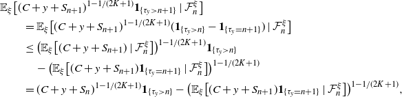 \begin{align*} & \mathbb{E}_{\xi}\big[(C+y+S_{n+1})^{1-{1}/({2K+1})}\mathbf{1}_{\{\tau_{y}>n+1\}}\mid\mathcal{F}^{\xi}_{n}\big] \\ & \qquad = \mathbb{E}_{\xi}\big[(C+y+S_{n+1})^{1-{1}/({2K+1})}(\mathbf{1}_{\{\tau_{y}>n\}}-\mathbf{1}_{\{\tau_{y}=n+1\}}) \mid \mathcal{F}^{\xi}_{n}\big] \\ & \qquad \leq \big(\mathbb{E}_{\xi}\big[(C+y+S_{n+1})\mid\mathcal{F}^{\xi}_{n}\big]\big)^{1-{1}/({2K+1})} \mathbf{1}_{\{\tau_{y}>n\}} \\ & \qquad\quad - \big(\mathbb{E}_{\xi}\big[(C+y+S_{n+1})\mathbf{1}_{\{\tau_{y}=n+1\}} \mid \mathcal{F}^{\xi}_{n}\big]\big)^{1-{1}/({2K+1})} \\ & \qquad = (C+y+S_{n})^{1-{1}/({2K+1})}\mathbf{1}_{\{\tau_{y}>n\}} - \big(\mathbb{E}_{\xi}\big[(C+y+S_{n+1})\mathbf{1}_{\{\tau_{y}=n+1\}}\mid\mathcal{F}^{\xi}_{n}\big]\big)^{1-{1}/({2K+1})}, \end{align*}
where the first inequality follows by Jensen’s inequality. For the second term in (10), we have
 \begin{align*} \mathbb{E}_{\xi}\big[|y+S_{\tau_y}|\mathbf{1}_{\{\tau_{y}\leq n+1\}}\mid\mathcal{F}^{\xi}_{n}\big] & = \mathbb{E}_{\xi}\big[|y+S_{\tau_y}|(\mathbf{1}_{\{\tau_{y}\leq n\}}+\mathbf{1}_{\{\tau_{y}=n+1\}}) \mid \mathcal{F}^{\xi}_{n}\big] \\ & = |y+S_{\tau_y}|\mathbf{1}_{\{\tau_{y}\leq n\}} + \mathbb{E}_{\xi}\big[|y+S_{n+1}|\mathbf{1}_{\{\tau_{y}=n+1\}}\mid\mathcal{F}^{\xi}_{n}\big]. \end{align*}
Now we can choose C and K sufficiently large that
 \begin{align*} \mathbb{E}_{\xi}\big[|y+S_{n+1}|\mathbf{1}_{\{\tau_{y}=n+1\}}\mid\mathcal{F}^{\xi}_{n}\big] - \big(\mathbb{E}_{\xi}\big[(C+y+S_{n+1})\mathbf{1}_{\{\tau_{y}=n+1\}}\mid\mathcal{F}^{\xi}_{n}\big]\big)^{1-{1}/({2K+1})} \leq 0. \end{align*}
In fact, for any
 $0<\eta<1$
, we can choose
 $N_3$
such that
 \begin{align*} \mathbb{E}_{\xi}(|X_{n+1}|\mathbf{1}_{\{|X_{n+1}|>N_3\}}) \leq \sum_{k=N_3}^{\infty}\mathbb{P}_{\xi}(|X_{n+1}|\geq k)<\eta. \end{align*}
Then, letting
 $C>2N_3$
and K large enough, it follows that
 \begin{align*} \mathbb{E}_{\xi}\big[|y+S_{n}+X_{n+1}|\mathbf{1}_{\{\tau_{y}=n+1\}}\mid\mathcal{F}^{\xi}_{n}\big] \leq \big(\mathbb{E}_{\xi}\big[(C+y+S_{n}+X_{n+1})\mathbf{1}_{\{\tau_{y}=n+1\}} \mid \mathcal{F}^{\xi}_{n}\big]\big)^{1-{1}/({2K+1})}. \end{align*}
Therefore, we obtain (9) immediately from the above arguments.
Proof of Theorem
2(ii). Note that
 $U(\xi,0)>0$
for almost all
 $\xi$
under the assumption
 $\mathbb{P}_\xi(X_1>0)>0$
P-a.s. For any
 $y>0$
, since
 $y+S_{\tau_{y}}<0$
, by (7) and the definition of
 $U_n(\xi,y)$
, we have, for any
 $n\geq1$
,
 $U_n(\xi,y)=y-\mathbb{E}_\xi(y+S_{\tau_{y}};\;\tau_{y}\leq n)\geq y$
. Taking the limit as
 $n\to\infty$
and using Theorem 1, we get
 $U(\xi,y)\geq y>0$
.
For any
 $y_1\leq y_2$
, we have
 $\tau_{y_1}\leq \tau_{y_2}$
. Therefore, for any
 $n\geq1$
,
 \begin{align*} \mathbb{E}_\xi(y_1+S_{n};\;\tau_{y_1}>n) \leq \mathbb{E}_\xi(y_2+S_{n};\;\tau_{y_1}>n) \leq \mathbb{E}_\xi(y_2+S_{n};\;\tau_{y_2}>n). \end{align*}
Taking the limit again, we get
 $U(\xi,y_1)\leq U(\xi,y_2)$
.
Since
 $f(y+S_{n\wedge\tau_y})$
is a non-negative supermartingale, for
 $y\geq0$
, by the optional stopping theorem,
 $\mathbb{E}_\xi|y+S_{\tau_y}|\leq (C+y)^{1-{1}/({2K+1})}$
. Indeed, by Fatou’s lemma and the supermartingale property,
 \begin{align*} \mathbb{E}_{\xi}|y+S_{\tau_y}| = \mathbb{E}_{\xi}\big[\lim_{n\to\infty}f(y+S_{n\wedge\tau_y})\big] & \leq \liminf_{n\to\infty}\mathbb{E}_{\xi}[f(y+S_{n\wedge\tau_y})] \\ & \leq \mathbb{E}_{\xi}[f(y+S_{0})] = (C+y)^{1-{1}/({2K+1})}. \end{align*}
This implies that
 $\lim_{y\to\infty}{-\mathbb{E}_\xi(S_{\tau_y})}/{y}=1$
. The proof of Theorem 2 is completed.
3.3. Proof of Corollary 1
Proof of Corollary
1(i). For any
 $B\in\mathcal{F}^{\xi}_{n}$
, by the quenched harmonic property and independence, we get
 \begin{equation*} \mathbb{E}_\xi[U(\theta^{n+1}\xi,y+S_{n+1})\mathbf{1}_{\{\tau_{y}>n+1\}}\mathbf{1}_B] = \mathbb{E}_\xi[U(\theta^n\xi,y+S_n)\mathbf{1}_{\{\tau_{y}>n\}}\mathbf{1}_B]. \end{equation*}
By the definition of conditional expectation, this equality implies that
 \begin{align*}\mathbb{E}_\xi\big[U(\theta^{n+1}\xi,y+S_{n+1})\mathbf{1}_{\{\tau_{y}>n+1\}}\mid\mathcal{F}^{\xi}_{n}\big] = U(\theta^n\xi,y+S_n)\mathbf{1}_{\{\tau_{y}>n\}},\end{align*}
which is the desired martingale property.
Proof of Corollary
1(ii). It follows from (2) that, for each
 $n\in\mathbb{N}^*$
and
 $y\geq0$
,
 \begin{equation*} \lim\limits_{y\to\infty}\frac{U(\theta^n\xi,y)}{y}=1 \quad \mathrm{P}\text{-a.s.} \end{equation*}
Using Egorov’s theorem, we have uniform convergence with positive probability, hence
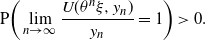 \begin{align*}\mathrm{P}\bigg(\lim\limits_{n\to\infty}\frac{U(\theta^n\xi,y_n)}{y_n}=1\bigg)>0.\end{align*}
Note that
 $\{\lim_{n\to\infty}{U(\theta^n\xi,y_n)}/{y_n}=1\}$
is a
 $\theta$
-invariant set and
 $\theta$
is ergodic by hypothesis; thus, we obtain
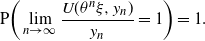 \begin{equation*} \mathrm{P}\bigg(\lim\limits_{n\to\infty}\frac{U(\theta^n\xi,y_n)}{y_n}=1\bigg)=1. \end{equation*}
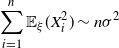
Proof of Corollary 1(iii). In our setting, the conditions of [Reference Denisov, Sakhanenko and Wachtel12, Theorem 1] hold and
 \begin{align*}\sum_{i=1}^n\mathbb{E}_{\xi}(X_i^2)\sim n\sigma^2\end{align*}
as
 $n\to\infty$
for almost every realization of
 $\xi$
, so we can obtain this claim using Theorem 1.
3.4. Proof of Theorem 3
Proof of Theorem
3. For any
 $1\leq k\leq n$
, conditioning on
 $\mathcal{F}^{\xi}_{k}$
, we have
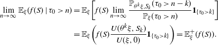
 \begin{align*} \mathbb{E}_{\xi}(f(S)\mid\tau_0>n) = \frac{\mathbb{E}_{\xi}(f(S)\mathbb{P}_{\theta^k\xi,S_k}(\tau_{0}>n-k) \mathbf{1}_{\{\tau_0>k\}})}{\mathbb{P}_{\xi}(\tau_0>n)}. \end{align*}
Then, by (3), (4), Lemma 3, and the dominated convergence theorem,
 \begin{align*} \lim_{n\to\infty}\mathbb{E}_{\xi}(f(S)\mid\tau_0>n) & = \mathbb{E}_{\xi}\bigg[f(S)\lim_{n\to\infty}\frac{\mathbb{P}_{\theta^k\xi,S_k}(\tau_{0}>n-k)} {\mathbb{P}_{\xi}(\tau_0>n)}\mathbf{1}_{\{\tau_0>k\}}\bigg] \\ & = \mathbb{E}_{\xi}\bigg(f(S) \frac{U(\theta^k\xi,S_k)}{U(\xi,0)} \mathbf{1}_{\{\tau_0>k\}}\bigg) = \mathbb{E}^+_{\xi}(f(S)). \end{align*}
Acknowledgements
We wish to thank the anonymous referees for their valuable comments, which improved the original manuscript.
Funding information
This work was supported in part by NSFC (No. 11971062), the National Key Research and Development Program of China (No. 2020YFA0712900), and the China Postdoctoral Science Foundation (No. 2024M761272).
Competing interests
There were no competing interests to declare which arose during the preparation or publication process of this article.


