2. Main result

Consider a filtered probability space $({\Omega},\mathcal{F}',(\mathcal{F}'_t)_{t\geq0},\mathbb{P})$ together with a smaller ${\sigma}$-field $\mathcal{F}$ and a smaller filtration $(\mathcal{F}_t)_{t\geq0}$ satisfying $\mathcal{F}_t\subseteq \mathcal{F}'_t\cap \mathcal{F}$ for all $t\geq0$. Our assumptions on the ingredients of (1.2) and (1.3) are as follows.

Our goal is to consistently estimate H based on equally spaced high-frequency noisy observations $\{Y_{i/n}\colon i=0,\dots,\lfloor nT\rfloor\}$ of X, where $T>0$ is a finite time horizon and n is the number of observations per unit time. From our estimation procedure, we also obtain estimators of $C_t=\int_0^T {\sigma}_t^2\,\mathrm{d}t$ and $\Pi_t = \int_0^T \rho_t^2\,\mathrm{d}t$, the integrated volatility and integrated noise volatility. In order to mitigate the impact of the noise $Z_t$, we rely on the pre-averaging approach of [Reference Jacod, Li, Mykland, Podolskij and Vetter18, Reference Podolskij and Vetter21]. To this end, we choose a weight function $g\colon[0,1] \rightarrow \mathbb{R}$ and a window size $k_n = {n^\kappa}/{\theta}$, where $\theta,\kappa>0$ are tuning parameters. Given a function W, random or not (but we have $W=Y$ in mind), we write $g^n_j = g ({j}/{k_n})$ and define

(2.1) \begin{equation} \begin{aligned} \overline{W}(g)^n_i & = \sum_{j=1}^{k_n-1}g^n_j\big(W_{({i+j-1})/{n}} - W_{({i+j-2})/{n}}\big) = \sum_{j=1}^{k_n-1}g^n_j\Delta_{i+j-1}^n W, \\ \widehat{W}(g)^n_i & = \sum_{j=1}^{k_n}(g^n_j - g^n_{j-1})^2(\Delta_{i+j-1}^n W)^2 = \sum_{j=1}^{k_n}(\Delta g^n_j)^2(\Delta_{i+j-1}^n W)^2. \end{aligned}\end{equation}

The former expression is a weighted average of the increments of W (hence the name ‘pre-averaging’), which we consider for $W=Y=X+Z$ in order to smooth out the noise component Z while preserving the signal component X. Our main functionals of interest are given by

(2.2) \begin{equation} V(g)^{n,f}_T(Y) = \frac{1}{n}\sum_{i=1}^{\lfloor nT\rfloor}f\bigg(\frac{\overline{Y}(g)^n_i}{(k_n/n)^H}, \frac{\widehat{Y}(g)^n_i}{(k_n/n)^{2H}}\bigg)\end{equation}

for some test function $f\colon\mathbb{R}^2 \to \mathbb{R}$. The following theorem is our main technical result.

Theorem 2.1. In the setting of Assumption 2.1, further suppose that $g\colon[0,1] \rightarrow \mathbb{R}$ is $C^2$ with $g(0)=g(1)=0$ and $f\colon\mathbb{R}^2 \rightarrow \mathbb{R}$ is $C^2$ with all partial derivatives up to order two of at most polynomial growth. Then, for any $T>0$, $\theta>0$ and $\kappa\in[{2H}/({2H+1}),1)$, we have the convergence

(2.3) \begin{equation} V(g)^{n,f}_T(Y) \overset{\mathbb{P}}{\longrightarrow} V(g)^{f}_T(Y) = \int_0^T\mu_f\bigg(\sigma_s^2\eta(g),\Theta^{2H+1}\rho_s^2\int_0^1g'(r)^2\,\mathrm{d}r\bigg)\,\mathrm{d}s, \end{equation}

where

(2.4) \begin{equation} \mu_f(v_1,v_2) = \mathbb{E}[f(\sqrt{v_1}Z_1 + \sqrt{v_2}Z_2, 2v_2)] \end{equation}

with independent $Z_1, Z_2 \sim N(0,1)$ and

(2.5) \begin{equation} \Theta = \begin{cases} 0, & \kappa \neq \dfrac{2H}{2H+1}, \\[8pt] \theta, & \kappa = \dfrac{2H}{2H+1}, \end{cases}\qquad \eta(g) = -\frac12\int_0^1\int_0^1g'(y)\lvert y-x\rvert^{2H}g'(x)\,\mathrm{d}x\,\mathrm{d}y. \end{equation}

Next, we explain how Theorem 2.1 can be used to solve the original statistical problem. Note that $V(g)^{n,f}_T(Y)$ is not a statistic, as it involves the unknown parameter H. In order to circumvent this problem, we use a classical change-of-frequency approach [Reference Barndorff-Nielsen, Corcuera and Podolskij2, Reference Corcuera, Hedevang, Pakkanen and Podolskij11]. More precisely, we consider $f(x,y)=x^2-\frac12y$ and form the ratio statistic

(2.6) \begin{equation} R(g)^{n,2}_T(Y) = \frac{\sum_{i=1}^{\lfloor nT/2\rfloor}\big[(\overline{Y}(g)^{n/2}_{i})^{2}-\frac12\widehat Y(g)^{n/2}_i\big]} {\sum_{i=1}^{\lfloor nT\rfloor}\big[(\overline{Y}(g)^{n}_{i})^{2}-\frac12\widehat Y(g)^n_i\big]},\end{equation}

where the numerator is computed with one half of the original frequency (i.e. by taking increments of step size $2/n$).

Theorem 2.2. Given the assumptions of Theorem 2.1, the estimator

(2.7) \begin{equation} \widehat{H}_n = \frac{1}{2(1 - \kappa)}\big(1+\log_{2} R(g)^{n,2}_T(Y) \big) \end{equation}

is consistent for H, i.e. satisfies $\widehat{H}_n \to H$ in probability as $n \to \infty$.

Proof. Let $f(x,y)=x^2-\frac12 y$. By Theorem 2.1, both $V(g)^{n/2,f}_T(Y)$ and $V(g)^{n,f}_T(Y)$ converge in probability to the same limit. In conjunction with the fact that $k_n\sim n^\kappa/\theta$, we obtain

\begin{equation*} R(g)^{n,2}_T(Y) = \frac{(n/2)(2k_{n/2}/n)^{2H}V(g)^{n/2,f}_T(Y)}{n(k_n/n)^{2H}V(g)^{n,f}_T(Y)} \stackrel{\mathbb{P}}{\longrightarrow} 2^{2H-1-2H\kappa}, \end{equation*}

from which we easily deduce that $\widehat{H}_n \to H$ in probability after applying the transform on the right-hand side of (2.7).

Next, we exhibit consistent estimators of $\Pi_t=\int_0^T \rho_t^2\,\mathrm{d}t$ and $C_T=\int_0^T{\sigma}_t^2\,\mathrm{d}t$, the respective integrated variance of noise and signal.

Proposition 2.1. We assume the hypotheses of Theorem 2.1. Furthermore, let $f(x,y)=x^2-\frac12 y$ and define

(2.8) \begin{align} \widehat{\Pi}^n_T & = \frac{1}{2\lfloor nT\rfloor}\sum_{i=1}^{\lfloor nT\rfloor}(Y_{{i}/{n}} - Y_{({i-1})/{n}})^{2} - \frac1{2Tn^{2\widehat H_n}}\widehat C^n_T, \end{align}

(2.9) \begin{align} \widehat C_T^n = \frac{1}{{\widehat \eta (g)}}\widehat V(g)_T^{n,F}(Y), \end{align}

where $\widehat V(g)_{T}^{n,F}(Y)$ and $\widehat{\eta}(g)$ are computed from (2.2) and (2.5), respectively, but with the estimator $\widehat{H}_n$ instead of H. Then, as $n\to\infty$, we have $\Pi^n_T\to \Pi_T$ and $\widehat C^n_T \to C_T$ in probability.

Proof. The convergence in (2.9) is a direct consequence of Theorem 2.1, Theorem 2.2, and the fact that $\mu_F(v_1,v_2) = v_1+v_2 - (2v_2)/2=v_1$. For (2.8), since $Y_{t} = X_{t} + \rho_t Z_{t}$, we may write the difference as $\Delta^n_i Y = \Delta^n_i X + \Delta^n_i \rho Z$. Squaring, we see that

\begin{equation*} \widehat\Pi^n_T = \Bigg(\frac{1}{2\lfloor nT\rfloor}\sum_{i=1}^{\lfloor nT\rfloor}(\Delta^n_i X)^2 - \frac1{2Tn^{2\widehat H_n}}\widehat C^n_T\Bigg) + \frac{1}{2\lfloor nT\rfloor}\sum_{i=1}^{\lfloor nT\rfloor}\Delta^n_i X \Delta^n_i \rho Z + \frac{1}{2\lfloor nT\rfloor}\sum_{i=1}^{\lfloor nT \rfloor}(\Delta^n_i \rho Z)^2. \end{equation*}

Since $\mathbb{E}[\lvert\Delta^n_i X\rvert^p]^{1/p}\lesssim\Delta_n^H$ (see Lemma 5.1), the first two terms are negligible (in particular, subtracting $(2Tn^{2\widehat H_n})^{-1}\widehat C^n_T$ in (2.8) is only a second-order correction) and we only need to determine the limit of $({1}/{2\lfloor nT\rfloor})\sum_{i=1}^{\lfloor nT\rfloor}(\Delta^n_i\rho Z)^2$. Conditionally on $\mathcal{F}$, $(\Delta^n_i \rho Z)_{i\in\mathbb{N}}$ is a 1-dependent sequence (i.e. $\Delta^n_i \rho Z$ and $\Delta^n_j \rho Z$ are $\mathcal{F}$-conditionally independent for any $\lvert i-j\rvert>1$). Thus, it converges to $\Pi_T$ by an application of the weak law of large numbers.

Our estimator of H depends on a choice of $\kappa\in [{2H}/({2H+1}),1]$. In recent work [Reference Szymanski and Takabatake24], it was shown in a parametric setting that the optimal rates of convergence for estimating H, $C_T$, and $\Pi_T$ are $n^{1/(4H+2)}$, $n^{1/(4H+2)}/\log n$, and $n^{1/2}$, respectively. Although we cannot prove it, we conjecture that choosing $\kappa_{\mathrm{opt}}={2H}/({2H+1})$ yields a rate-optimal estimator of H in the nonparametric framework considered here. Of course, taking $k_n= n^{\kappa_{\mathrm{opt}}}/\theta$ directly is impossible as we do not know H. To solve this problem and choose a sequence that is asymptotically of order $n^{\kappa_{\mathrm{opt}}}$, we could, in principle, follow the ideas outlined in [Reference Chong, Hoffmann, Liu, Rosenbaum and Szymanski9, Reference Chong, Hoffmann, Liu, Rosenbaum and Szymansky10, Reference Szymanski23]. But since optimality is not the main focus of this work, we do not present the details here. In the simulation and empirical sections below, we follow a more ad hoc approach, which yields sufficiently good estimates of H throughout the interval (0,1).

However, estimating $C_T$ and $\Pi_T$ is harder, especially as $H\to0$. This is in spite of a similar (in the case of $C_T$) or better (in the case of $\Pi_T$) rate of convergence. The intuition is that as $H\to0$, the increments of fractional Brownian motion approach an MA(1) process, with the consequence that the fractional part can no longer be distinguished from the noise part.

Theorem 2.3. Assume that ${\sigma}_t \equiv{\sigma}$ and $\rho_t\equiv\rho$, and let $(a_n)_{n\in\mathbb{N}}$ be any given null sequence. It is impossible to find a sequence $\widehat\theta_n$ of estimators of $\theta=({\sigma}^2,\rho^2)$ that achieves a rate of convergence of $a_n^{-1}$ uniformly over small H. That is, for any $\theta_0=\big({\sigma}^2_0,\rho^2_0\big)\in(0,\infty)^2$, there is $c>0$ such that $\limsup_{n\to\infty}\inf_{\widehat\theta_n}\sup_{(H,\theta)\in D_n(\theta_0)} \mathbb{P}_{(H,\theta)}(\lVert\widehat\theta_n - \theta\rVert > ca_n) > 0$, where the infimum is taken over all measurable functions $\widehat\theta_n$ of the data and

$$ D_n(\theta_0) = \{(H,{\sigma}^2,\rho^2)\colon H\in(0,1/\log a_n^{-1}),\ \lvert{\sigma}^2-{\sigma}_0^2\rvert \leq 1/\log a_n^{-1},\ \lvert \rho^2-\rho_0^2\rvert\leq1/\log a_n^{-1}\}. $$

As a consequence, for a given sample size n, the performance of any estimator of $({\sigma}^2,\rho^2)$ necessarily deteriorates as $H\to0$. This result is not in contradiction to the findings of [Reference Szymanski and Takabatake24], as the rates of convergence obtained there are only uniform in H on compact intervals within (0,1).

Proof of Theorem 2.3. Let $H_n\in(0,1)$ be a null sequence, to be determined later, and $r_n = a_n$. We define $\theta_n = ({\sigma}_0^2-r_n,\rho_0^2+r_n/2)$. Arguing as in the proof of [8, Theorem 4.1], it suffices to show that $\mathrm{KL}(\theta_n\parallel\theta_0) \leq \frac19$, where $\mathrm{KL}(\theta_n\parallel\theta_0)$ is the Kullback–Leibler divergence between the distribution of $\{\Delta^n_i Y\colon i=1,\dots,\lfloor nT\rfloor\}$ when the true parameters are $(H_n,\theta_n)$ and the distribution of $\{\Delta^n_i Y\colon i=1,\dots,\lfloor nT\rfloor\}$ when the true parameters are $(H_n,\theta_0)$. Because $\Delta^n_i Y$ is a centered stationary Gaussian time series, we have

$$ \mathrm{KL}(\theta_n\parallel\theta_0) = \frac12\bigg\{ \mathrm{tr}\big({\Sigma}_{0,n}^{-1}{\Sigma}_{1,n}\big) - n + \log\frac{\det{\Sigma}_{0,n}}{\det{\Sigma}_{1,n}}\bigg\}, $$

where

\begin{align*} {\Sigma}_{0,n} & = {\sigma}_0^2n^{-2H_n} {\Gamma}_n(H_n) + 2\rho^2_0{\Gamma}_n(0), \\ {\Sigma}_{1,n} & = \big({\sigma}_0^2-r_n\big)n^{-2H_n}{\Gamma}_n(H_n)+\big(2\rho_0^2+r_n\big){\Gamma}_n(0), \end{align*}

and

$$ {\Gamma}_n(H) = \big({\Gamma}^H_{\lvert i-j\rvert}\big)_{i,j=1}^n, \qquad {\Gamma}^H_r = \begin{cases} \frac12\big((r+1)^{2H}-2r^{2H}+(r-1)^{2H}\big) & \text{if } r\geq2,\\ \frac12\big(2^{2H}-2\big) & \text{if } r=1,\\ 1 & \text{if } r=0. \end{cases} $$

Let ${\Sigma}_{h,n} = h{\Sigma}_{1,n} + (1-h){\Sigma}_{0,n}$ and $\delta_n = {\Sigma}_{1,n}-{\Sigma}_{0,n}$. By [Reference Chong, Delerue and Mies8, (7.1)], we have

$$ \mathrm{KL}(\theta_n\parallel\theta_0) \leq \frac14\sup_{h\in(0,1)} \mathrm{tr}({\Sigma}_{h,n}^{-1}\delta_n{\Sigma}_{h,n}^{-1}\delta_n). $$

By definition, ${\Sigma}_{h,n}\geq 2\rho^2_0{\Gamma}_n(0)$, where $A\leq B$ means that $B-A$ is nonnegative definite. Therefore, ${\Sigma}^{-1}_{h,n}\leq (2\rho_0^2)^{-1}{\Gamma}_n(0)^{-1}$ and, by [Reference Chong, Delerue and Mies8, Lemma 7.1], it follows that

\begin{equation*} \mathrm{KL}(\theta_n\parallel\theta_0) \leq \frac1{16\rho_0^4} \mathrm{tr}({\Gamma}_n(0)^{-1}\delta_n{\Gamma}_n(0)^{-1}\delta_n). \end{equation*}

Using the fact that the Frobenius norm $\lVert \cdot\rVert_{\mathrm{F}}$ is submultiplicative and the bound $\mathrm{tr}(AB)\leq \lVert A\rVert_{\mathrm{F}}\lVert B\rVert_{\mathrm{F}}$, we obtain

\begin{equation*} \mathrm{KL}(\theta_n\parallel\theta_0) \leq \frac1{16\rho_0^4} \lVert{\Gamma}_n(0)^{-1}\delta_n\rVert_{\mathrm{F}}^2 \leq \frac1{16\rho_0^4}\lVert{\Gamma}_n(0)^{-1}\rVert_{\mathrm{F}}^2\lVert\delta_n\rVert_{\mathrm{F}}^2. \end{equation*}

By [Reference Hu and O’Connell17, (13)], there is $C>0$ such that $\lvert {\Gamma}_n(0)^{-1}_{ij}\rvert \leq Cn$ for all $n\in\mathbb{N}$ and $i,j=1,\dots,n$. Therefore, $\lVert {\Gamma}_n(0)^{-1}\rVert_{\mathrm{F}}\leq Cn^{2}$ and

$$\mathrm{KL}(\theta_n \parallel \theta_0) \leq \frac{C^2n^4}{16\rho_0^4}\lVert\delta_n\rVert_{\mathrm{F}}^2.$$

By definition, $\delta_n= r_n({\Gamma}_n(0)-{\Gamma}_n(H_n)) + r_n(1-n^{-2H_n}){\Gamma}_n(H_n)$. Because all entries of ${\Gamma}_n(H)$ are in $[{-}1,1]$, we have $\lVert{\Gamma}_n(H_n)\rVert_{\mathrm{F}} \leq n$ and $\lVert\delta_n\rVert_{\mathrm{F}} \leq \lVert{\Gamma}_n(0)-{\Gamma}_n(H_n)\rVert_{\mathrm{F}} + 2nH_n\log n$. For any $H\in[0,1)$, ${\Gamma}_n(H)$ is the $n\times n$ Toeplitz matrix generated by the associated spectral density, i.e. ${\Gamma}_n(H)=\big(\int_{-\pi}^\pi f_H({\lambda}){\text{e}}^{i(j-k){\lambda}}\,\mathrm{d}{\lambda}\big)_{j,k=1}^n$, where

$$ f_H({\lambda}) = \begin{cases} \frac{{\Gamma}(2H+1)\sin(\pi H)}{\pi}(1-\cos{\lambda})\sum_{k\in\mathbb{Z}}\lvert{\lambda}+2k\pi\rvert^{-2H-1} & \text{if } H\in(0,1), \\ \frac{1-\cos{\lambda}}{2\pi} & \text{if } H=0. \end{cases} $$

A straightforward computation shows that $\sup_{{\lambda}\in(-\pi,\pi)}\lvert f_H({\lambda})-f_0({\lambda})\rvert=O(H)$ as $H\to0$. Therefore, $\lVert{\Gamma}_n(0)-{\Gamma}_n(H_n)\rVert_{\mathrm{F}} \leq C'nH_n$ and $\lVert\delta_n\rVert_{\mathrm{F}}\leq C'n H_n\log n$ for some $C'>0$. Choosing $H_n\leq 4\rho_0^2/(3CC'n^{3} \log n)$ yields $\mathrm{KL}(\theta_n \parallel \theta_0) \leq \frac19$, which completes the proof.

3. Monte Carlo simulations

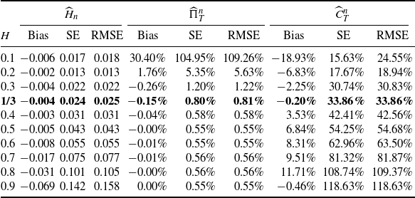
In this section, we document the finite-sample performance of our estimators from Section 2 based on 5000 simulated paths from the model

(3.1) \begin{equation} Y_t = {\sigma} B^H_t + \rho Z_t, \quad t\in[0,1],\end{equation}

for each of the values $H\in\big\{ 0.1, 0.2, 0.3, \tfrac13, 0.4, 0.5, 0.6, 0.7, 0.8, 0.9\big\}$. In (3.1), $B^H$ is a standard fractional Brownian motion with Hurst index H, $Z_t$ is standard Gaussian white noise, and ${\sigma}=1$, $\rho=0.1$. As a sampling frequency, we choose $n=100\,000$. Furthermore, we take $g(x) = 2(x \wedge (1 - x))$ as the weight function for pre-averaging. In order to obtain a window size $k_n$ that is as close as possible to the optimal rate $n^{2H/(2H+1)}$, we use an adaptive approach by first taking $k_n^{(0)}=n^{2/3}$, which corresponds to an admissible $\kappa$ for any value of $H\in(0,1)$. We then obtain an estimator $\widehat H_n^{(0)}$ of H using (2.7) and plug this value in to get a new window size $k_n^{(1)}=n^{2 \widehat H_n^{(0)}/(2\widehat H_n^{(0)}+1)}$. We then update our estimator of H to $\widehat H_n^{(1)}$ and subsequently compute a new window size $k_n^{(2)}$. This procedure is repeated until H no longer changes by more than a fixed threshold of $0.025$ or 100 iterations have been computed, whichever happens first. If an estimate of H is negative at some point in this procedure, we continue the iteration with $\kappa=0$. Throughout the estimation procedure, we ensure that the pre-averaging window size is always within $[30,n^{2/3}]$. To improve numerical stability, we further trim the subtrahend in both the numerator and the denominator of (2.6) at one half of the value of the respective minuend. Note that this does not alter the asymptotic limit of (2.6). With the final estimate of H, we then compute estimates of ${\sigma}^2$ and $\rho^2$ via (2.8) and (2.9).

Table 1 lists the bias, standard error (SE), and root mean square error (RMSE) of the resulting estimators. As we can see, the estimator of H performs well throughout the range of Hurst parameter values, with a slight increase in standard error as H approaches 1. This is in line with the findings of [Reference Szymanski and Takabatake24], where it was shown that the optimal rate of convergence for estimating H is $n^{1/(4H+2)}$ (which gets worse with larger H). The estimator of $\rho^2$ has good performance as well, except when H is very small. This, of course, is unavoidable given the result of Theorem 2.3. The errors in estimating ${\sigma}^2$, however, are nontrivial, both in terms of bias and standard error, for all values of H. In additional simulations (not reported here), we noticed that using a larger value of T (i.e. several days of data in practice) to estimate H significantly improves daily estimation of ${\sigma}^2$. In other words, a large proportion of the estimation error of $\widehat C^n_T$ is due to the uncertainty about H. Given that $\widehat H_n$ estimates H rather precisely, we conclude that $\widehat C^n_T$ is extremely sensitive to errors in estimating H.

Table 1.

Monte Carlo results based on 5,000 replications. For $\widehat C^n_T$ and $\widehat \Pi^n_t$, bias, SE, and RMSE are stated as a percentage of the true values. The row $H=\frac13$, highlighted in bold, is the case of interest in the turbulence application.

4. Application to turbulence data

To exemplify the performance of our estimators, we apply them to a dataset of 10 Hz temperature measurements collected at the Concordia Station (Dome C, Antarctica) on January 10, 2015, obtained from the IPEV/PNRA Project ‘Routin Meteorological Observation at Station Concordia’ (see http://www.climantartide.it). We also refer to [Reference Cheng, Li, Argentini, Sayde and Gentine5] for a more detailed description of the data. Under the hypothesis that temperature measurements satisfy Kolmogorov’s 2/3-law (or, in the spectral domain, Kolmogorov’s $-$5/3-law), we should see a roughness parameter $H=\frac13$ for a whole range of frequencies in the so-called inertial range. Thus, for each frequency $\Delta_n \in \{1\,\mathrm{s},\dots,30\,\mathrm{s}\}$ we split our dataset into hourly time series with increments of length $\Delta_n$ and compute, for each hour of January 10, 2015, estimates of H, volatility, and noise volatility in the same way as in the Monte Carlo simulation. Figure 1 shows the resulting estimates of H, C, and $\Pi$, obtained by averaging (for H) and taking the median of (for C and $\Pi$) the hourly estimates, as a function of $\Delta_n$. In particular, we find that, after removing the noise, the estimated roughness parameter of the data is, on average, in very good agreement with the theoretically predicted value of $H=\frac13$. On the other hand, if we do not perform pre-averaging (i.e. we choose $\kappa=0$), the estimates of H are practically 0 for all frequencies, indicating the presence of measurement noise in the data.

Figure 1.

Estimates of H without pre-averaging, and estimates of H, C, and $\Pi$ with pre-averaging for different sampling frequencies $\Delta_n$. In the first and second plots, the solid lines indicate the mean over all frequencies, while the dashed lines correspond to the hypothesized value of $H=\frac13$.

5. Proof of Theorem 2.1

Throughout this section, all the conditions in Theorem 2.1 are tacitly assumed. Also, by a standard localization argument (see, e.g., [19, Lemma 3.4.5]), we can additionally make the following assumptions:

• • The processes ${\sigma}$, a, and $\rho$ are uniformly bounded by a fixed constant. In particular, they possess uniformly bounded moments of all orders.

• • The processes ${\sigma}$, a, and $\rho$ are $L^p$-continuous for any $p>0$.

These two conditions will also be used without mentioning in what follows. We further write $A\lesssim B$ if there is $C\in(0,\infty)$, independent of anything important, such that $A\leq CB$. Notionally, if we say that a random variable has some size f(n), then all $L^p$-norms are bounded by a constant depending on p times f(n).

In the following we will make repeated use of the following $L^p$-estimates of the increments of $X^H$.

Lemma 5.1. Recall that $X^H_t = K_H^{-1}\int_0^t(t-s)^{H -1/2}\sigma_s\,d B_s$. For any $p>0$,

(5.1) \begin{equation} \big\|{\Delta^n_i X^H}\big\|_{L^{p}} \lesssim n^{-H}, \end{equation}

with a constant that does not depend on n or i.

Proof. For simplicity, we write $X^H_t = \int_0^t h(t-s)\sigma_s\,\mathrm{d}B_s$, where $h(t)=K_H^{-1}t^{H-1/2}_+$. Then, by the Burkholder–Davis–Gundy (BDG) inequality,

\begin{equation*} \big\|{\Delta^n_i X^H}\big\|_{L^{p}} \lesssim \mathbb{E}\bigg[\bigg|\int^{{i}/{n}}_0 \bigg(h\bigg(\frac{i}{n}-s\bigg)-h\bigg(\frac{i-1}{n}-s\bigg)\bigg)^2\sigma_s^2\, \mathrm{d}s\bigg|^{{p}/{2}}\bigg]^{{1}/{p}}. \end{equation*}

If $p\geq2$, we apply the Minkowski integral inequality to bound the previous line by

\begin{multline*} \bigg(\int_0^{i/n}\bigg(h\bigg(\frac{i}{n}-s\bigg)-h\bigg(\frac{i-1}{n}-s\bigg)\bigg)^2 \big\|{\sigma^2_s}\big\|_{L^{{p}/{2}}}\,\mathrm{d}s\bigg)^{{1}/{2}} \\ \lesssim \bigg(\int_0^{i/n}\bigg(h\bigg(\frac{i}{n}-s\bigg)-h\bigg(\frac{i-1}{n}-s\bigg)\bigg)^2\,\mathrm{d} s\bigg)^{{1}/{2}}, \end{multline*}

since $\sigma$ has uniformly bounded moments. Thus,

\begin{equation*} \big\|{\Delta^n_i X^H}\big\|_{L^{p}} \lesssim \bigg(\int_0^{i/n}\bigg(h(s)-h\bigg(s-\frac1n\bigg)\bigg)^2\,\mathrm{d}s\bigg)^{{1}/{2}} \leq n^{-H}\bigg(\int_0^\infty(h(s)-h(s-1)\big)^2\,\mathrm{d}s\bigg)^{{1}/{2}}, \end{equation*}

which shows (5.1) for $p\geq2$ since the last integral is finite. if $p < 2$, we simply apply Jensen’s inequality.

Next, we compute $L^p$-bounds on an averaged increment of $X^H$. The result motivates the choice of normalization in the definition of $V(g)_T^{n,f}(Y)$.

Proposition 5.1. For every $p\geq2$,

(5.2) \begin{equation} \big\|{\overline{X^H}(g)^n_i}\big\|_{L^{p}} \lesssim ({k_n}/{n})^H, \end{equation}

with a constant that does not depend on n or i.

Proof. Recall the notation in (2.1) for a general process W as well as $\Delta g^n_j = g^n_j-g^n_{j-1}$, with $g^n_{-1} = 0$. To get an idea of the proof, we consider the special case when $p=2$ first. We can apply summation by parts and obtain

\begin{equation*} \begin{split} \mathbb{E}\big[\big(\overline{X^H}(g)^n_i\big)^2\big] & = \mathbb{E}\Bigg[\Bigg(\sum_{j=1}^{k_n-1}g^n_j\Delta_{i+j-1}^nX^H\Bigg)^2\Bigg] \\ & = \mathbb{E}\Bigg[\Bigg(\sum_{j=1}^{k_n-1}\sum_{l=0}^{j}\Delta g^n_l\Delta_{i+j-1}^nX^H\Bigg)^2\Bigg] = \mathbb{E}\Bigg[\Bigg(\sum_{l=0}^{k_n-1}\Delta g^n_l\sum_{j=l}^{k_n-1}\Delta_{i+j-1}^nX^H \Bigg)^2\Bigg]. \end{split} \end{equation*}

By the Cauchy–Schwarz inequality,

\begin{align*} \mathbb{E}\Bigg[\Bigg(\sum_{l=0}^{k_n-1}\Delta g^n_l & \big(X^H_{({i+k_n-2})/{n}}-X^H_{({i+l-2})/{n}}\big)\Bigg)^2\Bigg] \\ & \leq 2\Bigg(\sum_{l=0}^{k_n-1}1\Bigg)\Bigg(\sum_{l=0}^{k_n-1} \mathbb{E}\big[(\Delta g^n_l)^2\big(X^H_{({i+k_n-2})/{n}}-X^H_{({i+l-2})/{n}}\big)^2\big]\Bigg) \\ & = 2k_n\sum_{l=0}^{k_n-1}(\Delta g^n_l)^2\mathbb{E}\big[\big(X^H_{({i+k_n-2})/{n}}-X^H_{({i+l-2})/{n}}\big)^2\big] \\ & \lesssim k_n\sum_{l=0}^{k_n-1}\frac{1}{k_n^2}(g'(\xi^n_l))^2\bigg(\frac{k_n-l}{n}\bigg)^{2H}, \end{align*}

where the last inequality follows from the mean-value theorem and Lemma 5.1. Recall that $g'$ is bounded, so this is bounded as

\begin{equation*} \mathbb{E}\Bigg[\Bigg(\sum_{l=0}^{k_n-1}\Delta g^n_l\big(X^H_{({i+k_n-2})/{n}}-X^H_{({i+l-2})/{n}}\big)\Bigg)^2\Bigg] \lesssim \frac{1}{k_n}\sum_{l=0}^{k_n-1}\bigg(\frac{k_n-l}{n}\bigg)^{2H} \leq \bigg(\frac{k_n}{n}\bigg)^{2H}, \end{equation*}

which is (5.2) for $p=2$.

Then we can extend this to $L^p$ with $p \geq2$ by using Hölder’s inequality and Lemma 5.1 to obtain

\begin{align*} \mathbb{E}\big[\big\lvert\overline{X^H}(g)^n_i\big\rvert^p\big] & \lesssim \mathbb{E}\Bigg[\Bigg|\sum_{l=0}^{k_n-1}\Delta g^n_l \big(X^H_{({i+k_n-2})/{n}}-X^H_{({i+l-2})/{n}}\big)\Bigg|^p\Bigg] \\ & \leq k_n^{p-1}\sum_{l=0}^{k_n-1}\lvert\Delta g^n_l\rvert^p \mathbb{E}\big[\big|X^H_{({i+k_n-2})/{n}}-X^H_{({i+l-2})/{n}}\big|^p\big] \\ & \lesssim k_n^{p-1}\sum_{l=0}^{k_n-1}\bigg|\frac{g'(\xi^n_l)}{k_n}\bigg|^p\bigg(\frac{k_n-l}{n}\bigg)^{pH} \lesssim \bigg(\frac{k_n}{n}\bigg)^{pH}. \end{align*}

The next goal is to remove the drift A, that is, we show that we can safely work with only the fractional component $X^H_t$ of $X_t$.

Lemma 5.2. Letting $U_t = Y_t - X_0 - A_0 = X_t^H + \rho_t Z_t$,

\begin{equation*} \lim_{n \rightarrow \infty} \big\|{V(g)^{n,f}_T(Y) - V(g)^{n,f}_T(U)}\big\|_{L^{p}} = 0. \end{equation*}

Proof. Recalling the definition of the variation, the difference is really

\begin{equation*} \Bigg\|{\frac{1}{n}\sum_{i=1}^{\lfloor nT\rfloor}\bigg[f\bigg(\frac{\overline{Y}(g)^n_i}{(k_n/n)^H}, \frac{\widehat{Y}(g)^n_i}{(k_n/n)^{2H}}\bigg) - f\bigg(\frac{\overline{U}(g)^n_i}{(k_n/n)^H}, \frac{\widehat{U}(g)^n_i}{(k_n/n)^{2H}}\bigg)\bigg]}\Bigg\|_{L^{p}}. \end{equation*}

Applying the mean-value theorem to the difference, it becomes

\begin{equation*} \frac{1}{n}\sum_{i=1}^{\lfloor nT\rfloor} \begin{pmatrix}\partial_1 f(\xi^n_{1,i}) \\[2mm] \partial_2 f(\xi^n_{2,i}) \end{pmatrix}^\top \begin{pmatrix} \dfrac{\overline{Y}(g)^n_i - \overline{U}(g)^n_i}{(k_n/n)^H} \\[3mm] \dfrac{\widehat{Y}(g)^n_i - \widehat{U}(g)^n_i}{(k_n/n)^{2H}} \end{pmatrix} \end{equation*}

for some intermediate $\xi^n_{1,i}$ and $\xi^n_{2,i}$. Proposition 5.1 and Lemma 5.3 show that $\xi^n_{1,i}$ and $\xi^n_{2,i}$ have uniformly bounded moments in n and i of all orders p. Since $\partial_1 f$ and $\partial_2 f$ are of polynomial growth, the same is true for $\partial_1 f(\xi^n_{1,i})$ and $\partial_2 f(\xi^n_{2,i})$. Thus, by an application of Hölder’s inequality, it suffices to show that the two differences in the previous display converge to 0 in $L^p$ for any $p>0$.

Since $\big\lVert{\Delta_{i+j-1}^n A}\big\rVert_{L^1} \lesssim n^{-1}$ by the boundedness of a, we have $\lVert{\overline{A}(g)^n_i}\rVert_{L^1} \lesssim {k_n}/{n}$. Thus,

\begin{equation*} \bigg\|{\frac{\overline{Y}(g)^n_i - \overline{U}(g)^n_i}{(k_n/n)^H}}\bigg\|_{L^{p}} = \bigg\|{\frac{\overline{A}(g)^n_i}{(k_n/n)^H}}\bigg\|_{L^{p}} \lesssim \bigg(\frac{k_n}{n}\bigg)^{1 - H}, \end{equation*}

which tends to 0 for any $\kappa \in(0, 1)$. For the other difference, we first bound

\begin{align*} \bigg\|{\frac{\widehat{Y}(g)^n_i - \widehat{U}(g)^n_i}{(k_n/n)^{2H}}}\bigg\|_{L^{p}} & = \Bigg\|{\frac{n^{2H}}{k_n^{2H}}\sum_{j=1}^{k_n}(\Delta g^n_i)^2\big(\big(\Delta^n_{i+j-1}Y\big)^2 - \big(\Delta^n_{i+j-1}U\big)^2\big)}\Bigg\|_{L^{p}} \\ & \leq \frac{n^{2H}}{k_n^{2H}}\sum_{j=1}^{k_n}(\Delta g^n_i)^2 \big(\big\|{(\Delta^n_{i+j-1}A)^2}\big\|_{L^{p}} + 2\big\|{\Delta^n_{i+j-1}A\Delta^n_{i+j-1}U}\big\||_{L^{p}}\big). \end{align*}

Clearly, $\big\lVert\big(\Delta_{i+j-1}^n A\big)^2\big\rVert_{L^1} \lesssim n^{-2}$. Since Z has uniformly bounded moments of all orders and $\rho$ is bounded, we can use Hölder’s inequality to get

\begin{align*} \big\|{\Delta^n_{i+j-1}A\Delta^n_{i+j-1}U}\big\|_{L^{p}} & \leq \big\|{\Delta^n_{i+j-1}A}\big\|_{L^{2p}}\big(\big\|{\Delta^n_{i+j-1}X^H}\big\|_{L^{2p}} + \big\|{\Delta^n_{i+j-1}\rho Z}\big\|_{L^{2p}}\big) \\ & \lesssim n^{-1}\bigg(\bigg(\frac{k_n}{n}\bigg)^H + C\bigg) \lesssim n^{-1}. \end{align*}

Using the standard bound $\lvert \Delta g^n_i\rvert \lesssim k_n^{-1}$, we conclude that

$$ \bigg\|{\frac{\widehat{Y}(g)^n_i - \widehat{U}(g)^n_i}{(k_n/n)^{2H}}}\bigg\|_{L^{p}} \lesssim \frac{n^{2H}}{k_n^{2H}}\sum_{j=1}^{k_n}\bigg(\frac{g'(\xi^n_i)}{k_n}\bigg)^2n^{-1} \leq \frac{n^{2H-1}}{k_n^{2H+1}}, $$

which, since $\kappa \geq {2H}/({2H + 1}) > ({2H-1})/({2H+1})$, converges to 0 as $n \rightarrow \infty$.

Note that the lower bound on $\kappa$ in Theorem 2.1 is not the most parsimonious choice possible just examining the previous proof; the next step we take justifies a lower bound of ${2H}/({2H+1})$ rather than $({2H-1})/({2H+1})$ for $\kappa$.

Lemma 5.3.

$$ \limsup_{n\rightarrow\infty}\bigg\|{\frac{\widehat{U}(g)^n_i}{(k_n/n)^{2H}}}\bigg\|_{L^{p}} \begin{cases} < \infty & \text{if } \kappa = {2H}/({2H+1}), \\ = 0 & \text{if } \kappa > {2H}/({2H+1}). \end{cases} $$

Proof. Because

(5.3) \begin{equation} \bigg\|{\frac{\widehat{X^H}(g)^n_i}{({k_n}/{n})^{2H}}}\bigg\|_{L^{p}} \leq \frac{n^{2H}}{k_n^{2H}}\sum_{j=1}^{k_n}|\Delta g^n_j|^2\big\|{\big(\Delta^n_{i+j-1}X^H\big)^2}\big\|_{L^{p}} \lesssim \frac{1}{k_n^{2H+1}} \rightarrow 0, \end{equation}

we only need to worry about the noise part, which can be bounded by

\begin{equation*} \bigg\|{\frac{\widehat{\rho Z}(g)^n_i}{(k_n/n)^{2H}}}\bigg\|_{L^{p}} \leq \frac{n^{2H}}{k_n^{2H}}\sum_{j=1}^{k_n}(\Delta g^n_j)^2\big\|{\big(\Delta_{i+j-1}^n \rho Z\big)^2}\big\|_{L^{p}} = \frac{n^{2H}}{k_n^{2H}}\sum_{j=1}^{k_n}\bigg(\frac{g'(\xi^n_i)}{k_n}\bigg)^2 \big\|{\big(\Delta_{i+j-1}^n\rho Z\big)^2}\big\|_{L^{p}}. \end{equation*}

Now, since $\rho$ is bounded and Z has uniformly bounded pth moments, the $L^p$-norm may vary with p, but not n, so the above is bounded by

(5.4) \begin{equation} C_p\frac{n^{2H}}{k_n^{2H}}\sum_{j=1}^{k_n}\bigg(\frac{g'(\xi^n_i)}{k_n}\bigg)^2 \lesssim \frac{n^{2H}}{k_n^{2H+1}}, \end{equation}

which implies the claim since $k_n \sim n^\kappa/\theta$.

In comparison with semimartingales, the problematic part of working with fractional processes is that the domain of integration in stochastic integrals stretches all the way from 0. In the semimartingale case (i.e. with $H = \frac{1}{2}$), we have that an increment $X^{1/2}_{t_2} - X^{1/2}_{t_1} = \int_{t_1}^{t_2} {\sigma}_s\,\mathrm{d}B_s$, but for $H\neq \frac12$, $X^H_{t_2} - X^H_{t_1} = K_H^{-1}\int_0^{t_2}\big[(t_2-s)^{H-{1}/{2}} - (t_1-s)_+^{H-{1}/{2}}\big]{\sigma}_s\,\mathrm{d}B_s$. What we would like to be able to do is to truncate this interval arbitrarily close to where we begin averaging, namely at ${i}/{n}$ in the case of $\overline{U}(g)^n_i$. To this end, we introduce truncated increments of $X^H$, defined as

\begin{equation*} \Delta_{i}^{n,\varepsilon} X^H = K_H^{-1}\int_{{i}/{n}-\varepsilon}^{{i}/{n}} \bigg[\bigg(\frac{i}{n}-s\bigg)^{H-{1}/{2}} - \bigg(\frac{i-1}{n}-s\bigg)_+^{H-{1}/{2}}\bigg]\sigma_s\,\mathrm{d} B_s,\end{equation*}

where ${\varepsilon}>0$ is a truncation parameter. Correspondingly, we define

\begin{equation*} \Delta_{i}^{n,\varepsilon}U = \Delta_{i}^{n,\varepsilon}X^H + \Delta_{i}^n\rho Z, \quad \overline{U}(g)^{n,{\varepsilon}}_i = \sum_{j=1}^{k_n-1}g^n_j\Delta_{i+j-1}^{n,{\varepsilon}}U, \quad \widehat{W}(g)^n_i = \sum_{j=1}^{k_n}(\Delta g^n_j)^2\big(\Delta_{i+j-1}^{n,{\varepsilon}}U\big)^2.\end{equation*}

In order for this truncation to be a reasonable endeavor, we need the error we are making to be small; the amount that we discard must vanish in the limit if we take $\varepsilon \rightarrow 0$.

Lemma 5.4. For any ${\varepsilon}>0$,

\begin{equation*} \limsup_{n\rightarrow\infty}\Bigg\|{V(g)^{n,f}_T(U) - \frac{1}{n}\sum_{i=\lfloor n\varepsilon\rfloor+1}^{\lfloor nT\rfloor}f\bigg(\frac{\overline{U}(g)^{n,\varepsilon}_i}{(k_n/n)^H}, \frac{\widehat{U}(g)^{n,\varepsilon}_i}{(k_n/n)^{2H}}\bigg)}\Bigg\|_{L^{p}} \lesssim \varepsilon. \end{equation*}

Proof. The difference is composed of two parts:

(5.5) \begin{gather} \frac{1}{n}\sum_{i=1}^{\lfloor n\varepsilon\rfloor}f\bigg(\frac{\overline{U}(g)^n_i}{(k_n/n)^H}, \frac{\widehat{U}(g)^n_i}{(k_n/n)^H}\bigg),\end{gather}

(5.6) \begin{gather} \frac{1}{n}\sum_{i=\lfloor n\varepsilon\rfloor+1}^{\lfloor nT\rfloor}\bigg[ f\bigg(\frac{\overline{U}(g)^{n}_i}{(k_n/n)^H},\frac{\widehat{U}(g)^{n}_i}{(k_n/n)^H}\bigg) - f\bigg(\frac{\overline{U}(g)^{n,\varepsilon}_i}{(k_n/n)^H},\frac{\widehat{U}(g)^{n,\varepsilon}_i}{(k_n/n)^H}\bigg)\bigg]. \end{gather}

The $f(\cdot)$ term in (5.5) is of size 1, since f is assumed to be of polynomial growth and we showed previously that the arguments are at worst of size 1. This shows that (5.5) is $\lesssim {\varepsilon}$. Next, we want to show that (5.6) converges to 0.

The mean-value theorem reduces (5.6) to

\begin{equation*} \frac{1}{n}\sum_{\lfloor n\varepsilon\rfloor+1}^{\lfloor nT\rfloor} \begin{pmatrix} \partial_1 f(\xi_{1,i}^n) \\[1mm] \partial_2 f(\xi_{2,i}^n) \end{pmatrix}^\top \begin{pmatrix} \dfrac{\overline{U}(g)^{n,\varepsilon}_i - \overline{U}(g)^{n}_i}{(k_n/n)^H} \\[3mm] \dfrac{\widehat{U}(g)^{n,\varepsilon}_i - \widehat{U}(g)^{n}_i}{(k_n/n)^{2H}} \end{pmatrix}. \end{equation*}

As seen before, the partial derivatives are of size 1, so all that matters is that the differences on the right go to 0. Explicitly,

\begin{align*} & \overline{U}(g)^{n}_i - \overline{U}(g)^{n,\varepsilon}_i \\ & \qquad = \sum_{j=1}^{k_n-1}g^n_i\big(\Delta_{i+j-1}^{n}U - \Delta_{i+j-1}^{n,\varepsilon}U\big) \\ & \qquad = K_H^{-1}\sum_{j=1}^{k_n-1}g^n_i\int_0^{({i+j-1})/{n}-\varepsilon}\bigg[\bigg(\frac{i+j-2}{n}-s\bigg)^{H-{1}/{2}} - \bigg(\frac{i+j-1}{n}-s\bigg)^{H-{1}/{2}}\bigg]\sigma_s\,\mathrm{d}B_s, \end{align*}

so, by the BDG inequality, the boundedness of ${\sigma}$ and the substitution $r = ({i+j-1})/{n}-s$,

\begin{align*} & \big\|{\overline{U}(g)^{n}_i - \overline{U}(g)^{n,\varepsilon}_i}\big\|_{L^{p}} \\ & \qquad \lesssim \bigg(\int_0^{({i+j-1})/{n}-\varepsilon}\bigg[\bigg(\frac{i+j-1}{n}-s\bigg)^{H-{1}/{2}} - \bigg(\frac{i+j-2}{n}-s\bigg)^{H-{1}/{2}}\bigg]^2\,\mathrm{d}s\bigg)^{{1}/{2}} \\ & \qquad = \bigg(\int_{\varepsilon}^{({i+j-1})/{n}}\bigg(r^{H-{1}/{2}}-(r-\frac1n)^{H-{1}/{2}}\bigg)^2\,\mathrm{d} r\bigg)^{{1}/{2}}. \end{align*}

By the mean-value theorem, it follows that

\begin{equation*} \big\|{\overline{U}(g)^{n}_i - \overline{U}(g)^{n,\varepsilon}_i}\big\|_{L^{p}} \lesssim n^{-1}\bigg(\int_\varepsilon^{\infty}r^{2H-3}\,\mathrm{d}r\bigg)^{{1}/{2}} \lesssim C({\varepsilon})n^{-1}. \end{equation*}

Normalizing by $(k_{n}/n)^{H}$, we get that

$$ \frac{\big\|{\overline{U}(g)^{n}_i - \overline{U}(g)^{n,\varepsilon}_i}\big\|_{L^{p}}}{(k_{n}/n)^{H}} \lesssim C({\varepsilon})n^{-(1-H)-\kappa H}\to0. $$

Next,

\begin{align*} \widehat{U}(g)^{n}_i - \widehat{U}(g)^{n,\varepsilon}_i & = \sum_{j=1}^{k_n-1}(\Delta g^n_i)^2\big(\big(\Delta_{i+j-1}^{n}U\big)^2 - \big(\Delta_{i+j-1}^{n,\varepsilon}U\big)^2\big) \\ & = \sum_{j=1}^{k_n-1}(\Delta g^n_i)^2\big(\Delta_{i+j-1}^{n}U - \Delta_{i+j-1}^{n,\varepsilon}U\big) \big(\Delta_{i+j-1}^{n}U + \Delta_{i+j-1}^{n,\varepsilon}U\big). \end{align*}

We just saw that $\Delta_{i+j-1}^{n}U - \Delta_{i+j-1}^{n,\varepsilon}U$ is of size $n^{-1}$, while $\Delta_{i+j-1}^{n}U + \Delta_{i+j-1}^{n,\varepsilon}U$ is of size 1. Thus, $\widehat{U}(g)^{n}_i - \widehat{U}(g)^{n,\varepsilon}_i $ is of size $k_n^{-1}n^{-1}$, which still goes to 0 after dividing by $(k_n/n)^{2H}$.

Our next step is to discretize $\sigma$ and remove the fractional portion from the second argument.

Lemma 5.5.

\begin{multline*} \lim_{\varepsilon\rightarrow0}\limsup_{n\rightarrow\infty}\Bigg\lVert\frac{1}{n} \sum_{i=\lfloor n\varepsilon\rfloor+1}^{\lfloor nT\rfloor}\bigg[ f\bigg(\frac{\overline{U}(g)^{n,\varepsilon}_i}{(k_n/n)^H},\frac{\widehat{U}(g)^{n,\varepsilon}_i}{(k_n/n)^{2H}}\bigg) \\ - f\bigg(\frac{\sigma_{{i}/{n}-\varepsilon}\overline{B^{H}}(g)^{n,\varepsilon}_i + \overline{\rho Z}(g)^n_i}{(k_n/n)^{H}}, \frac{\widehat{\rho Z}(g)^n_i}{(k_n/n)^{2H}}\bigg)\bigg]\Bigg\rVert_{L_p} = 0, \end{multline*}

where $B^{H}_t=K_H^{-1}\int_0^t (t-s)^{H-1/2}\,\mathrm{d}B_s$ is fractional Brownian motion with unit volatility.

Proof. Via the mean-value theorem, the difference becomes

\begin{equation*} \frac{1}{n}\sum_{i=\lfloor n\varepsilon\rfloor+1}^{\lfloor nT\rfloor} \begin{pmatrix} \partial_1 f(\xi_{1,i}^n) \\[1mm] \partial_2 f(\xi_{2,i}^n) \end{pmatrix}^\top \begin{pmatrix} \dfrac{\overline{X^H}(g)^{n,\varepsilon}_i-\sigma_{{i}/{n}-\varepsilon}\overline{B^{H}}(g)^{n,\varepsilon}_i}{(k_n/n)^H} \\[3mm] \dfrac{\widehat{U}(g)^{n,\varepsilon}_i - \widehat{\rho Z}(g)^{n}_i}{(k_n/n)^{2H}} \end{pmatrix}, \end{equation*}

where the exact values of $\xi^n_{1,i}$ and $\xi^{n}_{2,i}$ may be different from before. Again, all we care about are the differences

(5.7) \begin{equation} \frac{\overline{X^{H}}(g)^{n,\varepsilon}_i - \sigma_{{i}/{n}-\varepsilon}\overline{B^{\prime H}}(g)^{n,\varepsilon}_i}{(k_n/n)^H}, \qquad \frac{\widehat{U}(g)^{n,\varepsilon}_i - \widehat{\rho Z}(g)^{n}_i}{(k_n/n)^{2H}}. \end{equation}

In order to handle the first term in (5.7), we recall h from the proof of Lemma 5.1 and write

\begin{align*} & \overline{X^{H}}(g)_{i}^{n,\varepsilon} - \sigma_{{i}/{n}-\varepsilon}\overline{B^{H}}(g)^{n,\varepsilon}_{i} \\ & \qquad = \sum_{j=1}^{k_n-1}g_j^n\Delta^{n,\varepsilon}_{i+j-1}X^H - \sum_{j=1}^{k_n-1}g_j^n\sigma_{{i}/{n}-\varepsilon}\Delta^{n,\varepsilon}_{i+j-1}B^{H} \\ & \qquad = \sum_{j=1}^{k_n-1}g_j^n\int^{({i+j-1})/{n}}_{({i+j-1})/{n}-\varepsilon} \bigg(h\bigg(\frac{i+j-1}{n}-s\bigg) - h\bigg(\frac{i+j-2}{n}-s\bigg)\bigg) (\sigma_s - {\sigma}_{i/n-{\varepsilon}})\,\mathrm{d}B_s. \end{align*}

Recall that the lower bound in the above integral is a consequence of the truncation from the previous lemma, where we removed the integral from 0 to $({i+j-1})/{n}-{\varepsilon}$. Clearly, we could have only removed the integral from 0 to ${i}/{n}-{\varepsilon}$, leaving the portion from ${i}/{n}-{\varepsilon}$ to $({i+j-1})/{n}$. In other words, there is no harm in replacing the integral in the last display by

$$ \Delta^{n,\varepsilon}_{i,j}\widetilde{X^H} = \int^{({i+j-1})/{n}}_{{i}/{n}-\varepsilon} \bigg(h\bigg(\frac{i+j-1}{n}-s\bigg) - h\bigg(\frac{i+j-2}{n}-s\bigg)\bigg) (\sigma_s - {\sigma}_{i/n-{\varepsilon}})\,\mathrm{d}B_s, $$

and $\widetilde{X}^{H,n,\varepsilon}_{i}= X^{H n,\varepsilon}_{i} - \sigma_{{i}/{n}-\varepsilon}B^{\prime H n, \varepsilon}_{i}$. Then, similarly to the proof of Proposition 5.1,

\begin{equation*} \Bigg\|{\sum_{j=1}^{k_n-1}g_j^n\Delta^{n,\varepsilon}_{i,j}\widetilde{X^H}}\Bigg\|_{L^{p}} = \Bigg\|{\sum_{j=1}^{k_n-1}\sum_{l=0}^{j}\Delta g^n_l\Delta^{n,\varepsilon}_{i,j}\widetilde{X^H}}\Bigg\|_{L^{p}} \leq \Bigg\|{\sum_{l=0}^{k_n-1}\Delta g^n_l\sum_{j=l}^{k_n-1}\Delta^{n,\varepsilon}_{i,j}\widetilde{X^H}}\Bigg\|_{L^{p}}. \end{equation*}

By definition,

$$ \sum_{j=l}^{k_n-1}\Delta^{n,\varepsilon}_{i,j}\widetilde{X^H} = \int^{({i+k_n-2})/{n}}_{{i}/{n}-\varepsilon}\bigg(h\bigg(\frac{i+k_n-2}{n}-s\bigg)-h\bigg(\frac{i+l-2}{n}-s\bigg)\bigg) (\sigma_s - {\sigma}_{i/n-{\varepsilon}})\,\mathrm{d}B_s, $$

which is a truncated fractional increment over an interval of length $(k_n-\ell)/n$ with volatility ${\sigma}_s-{\sigma}_{i/n-{\varepsilon}}$. By Lemma 5.1 and the $L^p$-continuity of ${\sigma}$, we can therefore bound

$$ \Bigg\|{\sum_{j=l}^{k_n-1}\Delta^{n,\varepsilon}_{i,j}\widetilde{X^H}}\Bigg\|_{L^{p}} \lesssim \bigg(\frac{k_n}{n}\bigg)^{H}\phi_p(2{\varepsilon}), $$

where $\phi_p(\tau) = \sup_{s,t\in[0,T],\lvert s-t\rvert\leq\tau}\mathbb{E}[\lvert{\sigma}_t-{\sigma}_s\rvert^p]^{1/p}$ satisfies $\phi_p(\tau)\to0$ as $\tau\to0$. Applying Hölder’s inequality, we then get

\begin{align*} \Bigg\|{\sum_{l=0}^{k_n-1}\Delta g^n_l\sum_{j=l}^{k_n-1}\Delta^{n,\varepsilon}_{i,j}\widetilde{X^H}}\Bigg\|_{L^{p}} & \leq k_n^{1-1/p}\Bigg(\sum_{l=0}^{k_n-1}\lvert\Delta g^n_l\rvert^p \mathbb{E}\Bigg[\Bigg|\sum_{j=l}^{k_n-1}\Delta^{n,\varepsilon}_{i,j}\widetilde{X^H}\Bigg|^p\Bigg]\Bigg)^{{1}/{p}} \\ & \lesssim \bigg(\frac{k_n}{n}\bigg)^{H}\phi_p(2{\varepsilon}). \end{align*}

Dividing by $(k_n/n)^H$, we can first let $n\to\infty$ and then ${\varepsilon}\to0$ to show that the first term in (5.7) is negligible.

Regarding the second term in (5.7), we decompose

\begin{equation*} \widehat{U}(g)^{n,\varepsilon}_i - \widehat{\rho Z}(g)^{n}_i = \sum_{j=1}^{k_n}(\Delta g^n_j)^2\big(\Delta^n_{i+j-1} X^H\big)^2 + \sum_{j=1}^{k_n}(\Delta g^n_j)^2\big(\Delta^n_{i+j-1} X^H\big)\big(\Delta^n_{i+j-1}\rho Z\big). \end{equation*}

We have already shown in (5.3) that the first term divided by $(k_n/n)^{2H}$ converges to 0 in $L^p$. Applying the Cauchy–Schwarz inequality, we can bound the second term by

$$ \Bigg(\sum_{j=1}^{k_n}(\Delta g^n_j)^2\big(\Delta^n_{i+j-1} X^H\big)^2\Bigg)^{1/2} \Bigg(\sum_{j=1}^{k_n}(\Delta g^n_j)^2\big(\Delta^n_{i+j-1}\rho Z\big)^2\Bigg)^{1/2}, $$

so (5.3) and (5.4) imply that the second term is also negligible.

The advantage of having both truncated the fractional increments and discretized ${\sigma}$ is that we can now prove a law of large numbers.

Lemma 5.6.

\begin{multline*} \lim_{{\varepsilon}\to0}\limsup_{n\to\infty}\Bigg\lVert\frac{1}{n}\sum_{i=\lfloor n\varepsilon\rfloor+1}^{\lfloor nT\rfloor} \bigg\{f\bigg(\frac{\sigma_{{i}/{n}-\varepsilon}\overline{B^H}(g)^{n,\varepsilon}_i + \overline{\rho Z}(g)^n_i}{(k_n/n)^{2H}}, \frac{\widehat{\rho Z}(g)^n_i}{(k_n/n)^{2H}}\bigg) \\ - \mathbb{E}\bigg[f\bigg(\frac{\sigma_{{i}/{n}-\varepsilon}\overline{B^{H}}(g)^{n,\varepsilon}_i + \overline{\rho Z}(g)^n_i}{(k_n/n)^{H}}, \frac{\widehat{\rho Z}(g)^n_i}{(k_n/n)^{2H}}\bigg) \mid \mathcal{F}_{{i}/{n}-\varepsilon}\bigg] \bigg\}\Bigg\rVert = 0. \end{multline*}

Proof. Abbreviate $f(\cdot)$ to $f_{i}$. We have to show that

\begin{equation*} \lim_{{\varepsilon}\to0}\limsup_{n\to\infty}\mathbb{E}\Bigg[\Bigg(\sum_{i=\lfloor n{\varepsilon}\rfloor+1}^{\lfloor nT\rfloor} \big\{f_i - \mathbb{E}[f_i \mid \mathcal{F}_{{i}/{n}-\varepsilon}]\big\}\Bigg)^2\Bigg] = 0. \end{equation*}

Developing the square, this becomes

(5.8) \begin{equation} \frac{1}{n^2}\sum_{i,j=\lfloor n\varepsilon\rfloor+1}^{\lfloor nT\rfloor}\mathbb{E}\big[ \big\{f_i - \mathbb{E}[f_i \mid \mathcal{F}_{{i}/{n}-\varepsilon}]\big\} \big\{f_j - \mathbb{E}[f_j \mid \mathcal{F}_{{j}/{n}-\varepsilon}]\big\}\big]. \end{equation}

By conditioning, we can see that as soon as $({i}/{n}-\varepsilon, ({i+k_{n}})/{n})$ and $({j}/{n}-\varepsilon, ({j+k_{n}})/{n})$ become disjoint, then this covariance is actually 0. So in (5.8), at most $\lfloor nT\rfloor\times(2k_n+2n{\varepsilon})$ terms are non-zero. Bounding each non-zero term by $\mathbb{E}[f_i^2]\leq C$, we can bound (5.8) by $({1}/{n^2}) \times \lfloor nT \rfloor \times (2 k_n + 2n\varepsilon) \times C \sim C\varepsilon \rightarrow 0$ as $\varepsilon \rightarrow 0$.

The next lemma calculates the conditional expectations arising in the law of large numbers.

Lemma 5.7. Recalling the function $\mu_f$ from (2.4), we have

\begin{multline*} \lim_{{\varepsilon}\to0}\limsup_{n\rightarrow\infty}\sum_{i=\lfloor n\varepsilon\rfloor+1}^{\lfloor nT\rfloor} \Bigg\{\mathbb{E}\bigg[f\bigg(\frac{\sigma_{{i}/{n}-\varepsilon}\overline{B^{H}}(g)^{n,\varepsilon}_i + \overline{\rho Z}(g)^n_i}{(k_n/n)^{H}}, \frac{\widehat{\rho Z}(g)^n_i}{(k_n/n)^{2H}}\bigg) \mid \mathcal{F}_{({i-1})/{n}-\varepsilon}\bigg] \\ \times \mu_f\Bigg(\frac{\sigma^2_{{i}/{n}-\varepsilon}}{k_n^{2H}}\sum_{j,l=1}^{k_n-1}g^n_jg^n_l\Gamma^H_{|j-l|}, \frac{\rho^2_{i/n-{\varepsilon}}}{(k_n/n)^{2H}}\sum_{j=1}^{k_n}(\Delta g^n_j)^2\Bigg)\Bigg\} = 0, \end{multline*}

where ${\Gamma}^H_r = \frac12\big((r+1)^{2H}-2r^{2H}+\lvert r-1\rvert^{2H}\big)$, $r\geq0$, is the autocorrelation function of the increments of a standard fractional Brownian motion.

Proof. We first pass to the limit in the second argument, by showing that

\begin{multline*} \lim_{{\varepsilon}\to0}\limsup_{n\rightarrow\infty}\sum_{i=\lfloor n\varepsilon\rfloor+1}^{\lfloor nT\rfloor}\mathbb{E}\Bigg[ \Bigg(f\bigg(\frac{\sigma_{{i}/{n}-\varepsilon}\overline{B^H}(g)^{n,\varepsilon}_i + \overline{\rho Z}(g)^n_i}{(k_n/n)^{H}}, \frac{\widehat{\rho Z}(g)^n_i}{(k_n/n)^{2H}}\bigg) \\ - f\Bigg(\frac{\sigma_{{i}/{n}-\varepsilon}\overline{B^H}(g)^{n,\varepsilon}_i + \overline{\rho Z}(g)^n_i}{(k_n/n)^{H}}, \frac{2\rho^{2}_{i/n-{\varepsilon}}}{(k_{n}/n)^{2H}}\sum_{j=1}^{k_{n}}(\Delta g^{n}_{j})^{2}\Bigg)\Bigg) \mid \mathcal{F}_{{i}/{n}-\varepsilon}\Bigg] = 0. \end{multline*}

By using the mean-value theorem as before, it is sufficient to show that, as $n \rightarrow \infty$,

(5.9) \begin{align} & \lim_{n\to\infty}\mathbb{E}\Bigg[\Bigg|\frac{\widehat{\rho Z}(g)^{n}_{i}}{(k_{n}/n)^{2H}} - \frac{1}{(k_{n}/n)^{2H}}\sum_{j=1}^{k_{n}}(\Delta g^{n}_{j})^{2} \big(\rho^{2}_{(i+j-1)/n}+\rho^2_{(i+j-2)/n}\big)\Bigg|^2\Bigg] = 0, \end{align}

(5.10) \begin{align} & \lim_{{\varepsilon}\to0}\limsup_{n\to\infty}\mathbb{E}\Bigg[\Bigg| \frac{1}{(k_{n}/n)^{2H}}\sum_{j=1}^{k_{n}}(\Delta g^{n}_{j})^{2}\big(\rho^{2}_{(i+j-1)/n}+\rho^2_{(i+j-2)/n}\big) - \frac{2\rho^{2}_{i/n-{\varepsilon}}}{(k_{n}/n)^{2H}}\sum_{j=1}^{k_{n}}(\Delta g^{n}_{j})^{2}\Bigg|^2\Bigg] = 0. \end{align}

The second convergence is easy since the expectation in (5.10) is of order

$$\bigg(\bigg(\frac{n^{2H}}{k_n^{2H+1}}\bigg)\psi\bigg(\frac{k_n}{n}\bigg)+{\varepsilon}\bigg)^2,$$

which goes to 0 as $n\to\infty$, and ${\varepsilon}\to0$ since $\psi(\tau)=\sup_{s,t\in[0,T],\lvert t-s\rvert \leq \tau} \mathbb{E}[\lvert \rho^2_t-\rho^2_s\rvert] \to0$ as $\tau\to0$ by the $L^2$-continuity of $\rho$. For (5.9), we develop the square and obtain

\begin{equation*} \frac{n^{4H}}{k_{n}^{4H}}\sum_{j,l=1}^{k_{n}}(\Delta g^{n}_{j})^{2}(\Delta g^{n}_{l})^{2} \mathrm{Cov}\big(\big(\Delta_{i+j-1}^{n}\rho Z\big)^{2},\big(\Delta_{i+l-1}^{n}Z\big)^{2} \big). \end{equation*}

By the independence properties of $Z_t$, the covariance in the sum is 0 unless $|l - j| \leq 1$. Moreover, even if $|l-j|\leq 1$, the covariance is bounded by a constant. Thus, the last display is $\lesssim n^{4H}k_{n}^{-4H}k_{n}k_{n}^{-4}$ and $\Delta g^{n}_{i} \sim k_{n}^{-1}$, which tends to 0 for any $\kappa\geq {2H}/({2H+1})$.

To handle the first argument, observe that $\sigma_{{i}/{n}-\varepsilon}\overline{B^H}(g)^{n,\varepsilon}_i/{(k_n/n)^{H}}$ is $\mathcal{F}_{i/n-{\varepsilon}}$-conditionally Gaussian with mean 0 and variance

\begin{multline*} \textrm{Var}\Bigg(\frac{\sigma_{{i}/{n}-\varepsilon}}{(k_{n}/n)^{H}}\sum_{j=\lfloor n\varepsilon\rfloor+1}^{k_{n}-1}g^{n}_{j} \Delta_{i+j-1}^{n,\varepsilon}B^{H} \mid \mathcal{F}_{i/n-{\varepsilon}}\Bigg) \\ = \frac{\sigma^2_{{i}/{n}-\varepsilon}}{(k_{n}/n)^{2H}}\sum_{j,l=\lfloor n\varepsilon\rfloor+1}^{k_{n}-1}g^{n}_{j}g^{n}_{l} \textrm{Cov}\big(\Delta^{n,\varepsilon}_{i+j-1}B^{H},\Delta^{n,\varepsilon}_{i+l-1}B^{H}\big). \end{multline*}

In the same way we showed that we could truncate increments of $X^H$ or $B^H$ at level ${\varepsilon}$, we can also reverse this step and approximate the last display by

$$ \frac{\sigma^2_{{i}/{n}-\varepsilon}}{(k_{n}/n)^{2H}}\sum_{j,l=\lfloor n\varepsilon\rfloor+1}^{k_{n}-1}g^{n}_{j}g^{n}_{l} \textrm{Cov}\big(\Delta^{n,\varepsilon}_{i+j-1}B^{H},\Delta^{n,\varepsilon}_{i+l-1}B^{H}\big) \approx_n \frac{\sigma^2_{{i}/{n}-\varepsilon}}{k_n^{2H}}\sum_{j,l=\lfloor n\varepsilon\rfloor+1}^{k_n-1}g^n_jg^n_l\Gamma^H_{|j-l|}, $$

where the last step follows, for example, from [7, Lemma B.1]. In the last display $\approx_n$ means that the difference of the two sides goes to 0 in $L^1$ as $n\to\infty$.

At the same time,

(5.11) \begin{equation} \frac{\overline{\rho Z}(g)^n_i}{(k_n/n)^H} = \frac{n^H}{k_n^H}\sum_{j=1}^{k_n-1}g^n_j\Delta^n_{i+j-1}\rho Z \approx_{n,{\varepsilon}} \rho_{i/n-{\varepsilon}}\frac{n^H}{k_n^H}\sum_{j=1}^{k_n-1}g^n_j\Delta^n_{i+j-1}Z, \end{equation}

where $\approx_{n,{\varepsilon}}$ means that the difference of the two sides converges to 0 in $L^1$ as $n\to\infty$ and ${\varepsilon}\to0$. Since $\Delta g^n_j = g'(\xi^n_j)/k_n$, we have, by the central limit theorem and the assumption $g(0)=g(1)=0$,

\begin{align*} \sqrt{k_n}\sum_{j=1}^{k_n-1}g^n_j\Delta^n_{i+j-1}Z & = \sqrt{k_n}\Bigg(g^n_{k_n-1}Z_{i+k_n-2}-g^n_1Z_{i-1} - \sum_{j=1}^{k_n-1}\Delta g^n_jZ_{i+j-1}\Bigg) \\ & \stackrel{\mathrm{d}}{\longrightarrow} N\bigg(0,\int_0^1 g'(s)^2\,\mathrm{d}s\bigg). \end{align*}

If $\kappa>{2H}/{2H+1}$, it follows that (5.11) goes to 0 in probability; if $\kappa={2H}/{2H+1}$, (5.11) is $\mathcal{F}_{i/n-{\varepsilon}}$-conditional Gaussian with mean 0 and variance $\theta^{2H+1}\rho_{i/n-{\varepsilon}}^2 \int_0^1 g'(s)^2\,\mathrm{d}s$. Since the last expression is also approximated by $\rho_{i/n-{\varepsilon}}^2/(k_n/n)^{2H}\sum_{j=1}^{k_n} (\Delta g^n_j)^2$, the lemma is proved.

Finally, we pass to the limit asserted in (2.3).

Lemma 5.8.

\begin{multline*} \lim_{\varepsilon\rightarrow0}\limsup_{n\to\infty}\Bigg\lVert\frac{1}{n}\sum_{i=\lfloor n\varepsilon\rfloor+1}^{\lfloor nT\rfloor} \mu_f\Bigg(\frac{\sigma^2_{{i}/{n}-\varepsilon}}{k_n^{2H}}\sum_{j,l=1}^{k_n-1}g^n_jg^n_l\Gamma^H_{|j-l|}, \frac{\rho^2_{i/n-{\varepsilon}}}{(k_n/n)^{2H}}\sum_{j=1}^{k_n}(\Delta g^n_j)^2\Bigg) \\ - \int_0^T\mu_f\bigg(\sigma_{s}^2\eta(g), \Theta^{2H+1}\rho^2_s\int_0^1g'(r)^2\,\mathrm{d}r\bigg)\,\mathrm{d} s\Bigg\rVert_{L_p} = 0. \end{multline*}

Proof. The difference above is $I^{n}_1+I^{n}_2$, where

\begin{align*} I^{n}_1 & = \sum_{i=\lfloor n\varepsilon\rfloor+1}^{\lfloor nT\rfloor}\int_{({i-1})/{n}}^{{i}/{n}}\Bigg\{ \mu_f\Bigg(\frac{\sigma^2_{{i}/{n}-\varepsilon}}{k_n^{2H}}\sum_{j,l=1}^{k_n-1}g^n_jg^n_l\Gamma^H_{|j-l|}, \frac{\rho^2_{i/n-{\varepsilon}}}{({k_n}/{n})^{2H}}\sum_{j=1}^{k_n}(\Delta g^n_j)^2\Bigg) \\ & \qquad\qquad\qquad\qquad\quad - \mu_f\bigg(\sigma_{s}^2\eta(g), \Theta^{2H+1}\rho^2_s\int_0^1g'(r)^2\,\mathrm{d}r\bigg)\,\mathrm{d}s\Bigg\}, \\ I^n_2 & = -\int_0^{{\lfloor n\varepsilon\rfloor}/{n}}\mu_f\bigg(\sigma_{s}^2\eta(g), \Theta^{2H+1}\rho^2_s\int_0^1g'(r)^2\,\mathrm{d}r\bigg)\,\mathrm{d}s \\ & \quad - \int_{{\lfloor nT\rfloor}/{n}}^T\mu_f\bigg(\sigma_{s}^2\eta(g), \Theta^{2H+1}\rho_s^2\int_0^1g'(r)^2\,\mathrm{d}r\bigg)\,\mathrm{d}s. \end{align*}

Since the $\mu_f$ term is of size one, $I^n_2$ is of size $\varepsilon+1/n$ and thus asymptotically negligible.

Hence, we only need to show that $I^n_1$ goes to 0. By the mean-value theorem,

\begin{align*} I^n_1 & = \sum_{i=\lfloor n\varepsilon\rfloor+1}^{\lfloor nT\rfloor}\int_{({i-1})/{n}}^{{i}/{n}} \big(\partial_1\mu_f\big(\xi^n_{1,i}\big), \partial_2\mu_f\big(\xi_{2,i}^n\big)\big) \\ & \quad \times \Bigg(\frac{\sigma^2_{{i}/{n}-\varepsilon}}{k_n^{2H}} \sum_{j,l=1}^{k_n-1}g^n_jg^n_l\Gamma^H_{|j-l|} - \sigma_{s}^2\eta(g), \\ & \qquad\quad \frac{\rho^2_{i/n-{\varepsilon}}}{({k_n}/{n})^{2H}} \sum_{j=1}^{k_n}(\Delta g^n_j)^2 - \Theta^{2H+1}\rho^2_s\int_0^1 g'(r)^2\,\mathrm{d}r\Bigg)^T\,\mathrm{d}s. \end{align*}

Each partial derivative is of size one, so we only need to show that the differences vanish in $L^p$. To this end, because ${\sigma}^2_{i/n-{\varepsilon}} \to {\sigma}_s^2$ and $\rho^2_{i/n-{\varepsilon}}\to \rho^2_s$ in $L^p$ as $n\to\infty$ and ${\varepsilon}\to0$, uniformly on [0,T], it remains to show that

$$ \frac{1}{k_n^{2H}}\sum_{j,l=1}^{k_n-1}g^n_jg^n_l\Gamma^H_{|j-l|} \to \eta(g), \qquad \frac{1}{({k_n}/{n})^{2H}}\sum_{j=1}^{k_n}(\Delta g^n_j)^2 \to \Theta^{2H+1}\int_0^1 g'(r)^2\,\mathrm{d}r. $$

The second convergence was already shown in (5.11) and the subsequent display. The first one is of independent interest and will be shown in a separate lemma.

Proof. Let us write $\Gamma^H_{r}=\overline{\Gamma}^H_{r}-\overline{\Gamma}^H_{r-1}=\Delta\overline{\Gamma}^H_{r}$, with $\overline \Gamma^H_1=\frac12$. Using summation by parts, we have

\begin{align*} & \frac{1}{k_n^{2H}}\sum_{j = 1}^{k_n-1} g^n_jg^n_l\Gamma^H_{|j-l|} \\ & \qquad = \frac{1}{k_n^{2H}}\sum_{j=1}^{k_n-1}(g^n_j)^2 + \frac{2}{k_n^{2H}}\sum_{j=1}^{k_n-2}g^n_j\Bigg(\sum_{l=j+1}^{k_n-1}g^n_l\Delta\overline{\Gamma}^H_{l-j}\Bigg) \\ & \qquad = \frac{1}{k_n^{2H}}\sum_{j=1}^{k_n-1}(g^n_j)^2 + \frac{2}{k_n^{2H}}\sum_{j=1}^{k_n-2}\Bigg(g^n_jg^n_{k_n-1}\overline{\Gamma}^H_{k_n-1-j} - \frac{1}{2}g^n_jg^n_{j+1} - \sum_{l=j+1}^{k_n-2}g^n_j\Delta g^n_{l+1}\overline{\Gamma}^H_{l-j}\Bigg) \\ & \qquad = \frac{1}{k_n^{2H}}\sum_{j=1}^{k_n-1}g^n_j(g^n_j-g^n_{j+1}) + \frac{2}{k_n^{2H}}\sum_{j=1}^{k_n-2}g^n_j g^n_{k_n-1}\overline{\Gamma}^H_{k_n-1-j} - \frac{2}{k_n^{2H}}\sum_{j=1}^{k_n-3}\sum_{l=j+1}^{k_n-2}g^n_j\Delta g^n_{l+1}\overline{\Gamma}^H_{l-j}. \end{align*}

By the mean-value theorem, the first term can be written as

\begin{align*} -\frac{1}{k_n^{2H}}\sum_{j=1}^{k_n-1}g^n_j\Delta g^n_{j+1} & = -\frac{1}{k_n^{2H}}\sum_{j=1}^{k_n-1}g\bigg(\frac{j}{k_n}\bigg) \bigg(g\bigg(\frac{j+1}{k_n}\bigg) - g\bigg(\frac{j}{k_n}\bigg)\bigg) \\ & = -\frac{1}{k_n^{2H+1}}\sum_{j=1}^{k_n-1}g\bigg(\frac{j}{k_n}\bigg){g'(\xi_j)}, \end{align*}

where $\xi_j \in ({j}/{k_n}, ({j+1})/{k_n})$. As $n\rightarrow\infty$, $(1/{k_n})\sum_{j=1}^{k_n-1}g({j}/{k_n}){g'(\xi_j)}\to\int_0^1g(x)g'(x)\,\mathrm{d}x$ by Riemann integration, so the term above vanishes as $k_n\rightarrow \infty$.

Similarly, since $\overline {\Gamma}^H_r = \frac12\big((r+1)^{2H}-r^{2H}\big)$, we have

\begin{align*} \frac{2}{k_n^{2H}}\sum_{j=1}^{k_n-2}g^n_j g^n_{k_n-1}\overline{\Gamma}^H_{k_n-1-j} & = \frac{1}{k_n^{2H}}\sum_{j=1}^{k_n-2}g^n_j g^n_{k_n-1}\big((k_n-j)^{2H} - (k_n-j-1)^{2H}\big) \\ & = \sum_{j=1}^{k_n-2}g^n_j g^n_{k_n-1}\bigg(\bigg(1-\frac{j}{k_n}\bigg)^{2H} - \bigg(1-\frac{j+1}{k_n}\bigg)^{2H}\bigg). \end{align*}

Let $h(x) \,:\!=\, (1-x)^{2H}$ and $h'(x) = -2H(1-x)^{2H-1}$. Then, again by Riemann integration,

\begin{align*} \frac{2}{k_n^{2H}}\sum_{j=1}^{k_n-2}g^n_j g^n_{k_n-1}\overline{\Gamma}^H_{k_n-1-j} & = \sum_{j=1}^{k_n-2}g^n_j g^n_{k_n-1}\bigg(h\bigg(\frac{j}{k_n}\bigg)^{2H} - h\bigg(\frac{j+1}{k_n}\bigg)^{2H}\bigg) \\ & = -\sum_{j=1}^{k_n-2}g^n_j g^n_{k_n-1}\frac{h'(\xi^n_j)}{k_n} \\ & \to 2Hg(1)\int_0^1g(x)(1-x)^{2H-1}\,\mathrm{d}x = 0. \end{align*}

Finally,

\begin{equation*} -\frac{2}{k_n^{2H}}\sum_{j=1}^{k_n-3}\sum_{l=j+1}^{k_n-2}g^n_j\Delta g^n_{l+1}\overline{\Gamma}^H_{l-j} = -\frac{1}{k_n^{2H}}\sum_{j=1}^{k_n-3}g^n_j\sum_{l=j+1}^{k_n-2}\big[(l-j+1)^{2H}-(l-j)^{2H}\big]\Delta g^n_{l+1}.\end{equation*}

Thus, by summation by parts, this term is equal to

\begin{align*} & -\frac{1}{k_n^{2H}}\sum_{j=1}^{k_n-3}g^n_j\Bigg(\Delta g^n_{k_n-1}(k_n-1-j)^{2H} - \Delta g^n_{j+2} - \sum_{l=j+1}^{k_n-3}(l-j+1)^{2H}(\Delta g^n_{l+2}-\Delta g^n_{l+1})\Bigg) \\ & \qquad = -\frac1{k_n}\sum_{j=1}^{k_n-3}\Bigg[g\bigg(\frac{j}{k_n}\bigg){g'\big(\xi^n_{k_n-1}\big)} \bigg(1-\frac{j+1}{k_n}\bigg)^{2H} - k_n^{-2H}g\bigg(\frac{j}{k_n}\bigg){g'\big(\xi^n_{j+2}\big)} \\ & \qquad\qquad\qquad\qquad - \frac{g({j}/{k_n})}{k_n}\sum_{l=j+1}^{k_n-3}\bigg(\frac{l-j+1}{k_n}\bigg)^{2H} {g''\big(\xi^n_{l+2}\big)}\Bigg] \\ & \qquad \to -g'(1)\int^1_0g(x)(1-x)^{2H}\,\mathrm{d}x + \int_0^1\int_x^1g(x)(y-x)^{2H}g''(y)\,\mathrm{d}y\,\mathrm{d}x. \end{align*}

Integrating by parts shows that the last line is equal to $-2H\int_0^1\int_x^1g(x)(y-x)^{2H-1}g'(y)\,\mathrm{d}y\,\mathrm{d}x$. Interchanging the $\mathrm{d}y$ and $\mathrm{d}x$ integrals and integrating by parts one more time results in the form of $\eta(g)$ stated in (2.5).