1. Introduction
As the field of modelling mortality has grown in recent years, the models proposed and used have grown ever more complicated. This has had the effect of increasing the number and importance of identifiability issues within the models, which can lead both to robustness problems when fitting the models to data and difficulties when projecting them. As the demands of modern longevity-risk management techniques require sophisticated models capable of capturing complex and subtle relationships between mortality rates across different ages and in different populations, unresolved identifiability issues have important practical consequences. We therefore believe that the time has come for a holistic and comprehensive analysis of the class of age/period/cohort (APC) mortality models and the identifiability issues within them.
In Hunt & Blake (Reference Hunt and Blake2020b), we analysed the structure of APC mortality models and proposed a way of classifying the models proposed to date. This gave us a general framework in which our study of identifiability issues operates. The existence of identifiability issues means that there are certain features of the parameters in a model which are not defined by the data. Instead, these features are only determined by the arbitrary identifiability constraints we impose upon the model when fitting it to data and, therefore, have no independent meaning. Consequently, we must be careful to ensure that our results from using mortality models do not depend upon these features of the parameters. In the context of the age/period (AP) mortality models discussed in this study, we find that features such as the levels of and correlations between the period terms and the scale of the age functions are unidentified by the models. These features therefore do not possess any meaning other than that imposed by our arbitrary identifiability constraints.
Identifiability issues arise in these mortality models because there exist different sets of parameters which will give the same fitted mortality rates. These identifiability issues can lead to models which lack robustness when fitted to data, cause us to draw faulty and erroneous conclusions when analysing the historical data and can bias our projected mortality rates in future. It is essential that we understand and resolve these issues when fitting models to data, as well as comprehend the impact these issues have on our analysis of past and future mortality rates.
Identifiability in mortality models is, therefore, a very important issue. While there are principles which are common to the vast majority of mortality models, the impact and implications of these issues vary considerably depending on the specifics of the model being used. To demonstrate these principles in action, we consider a number of simple models based on the classic and widely used models proposed in Lee & Carter (Reference Lee and Carter1992) and Cairns et al. (Reference Cairns, Blake and Dowd2006a), both of which are members of the class of AP models. In the particular cases chosen, the identifiability issues can appear trivial, and their impact on our analysis of historical and projected mortality rates relatively minor. However, we believe that it is vital to understand these issues fully in the context of simple models, since they become considerably more important in more sophisticated models, such as those constructed using the “general procedure” of Hunt & Blake (Reference Hunt and Blake2014).
In addition, due to the scale of the topic, this study deals only with the identifiability of AP mortality models. We leave the additional issues caused by the inclusion of a cohort term to Hunt & Blake (Reference Hunt and Blake2020a). Allowing for the dependence of mortality on year of birth in a model often creates new identifiability issues, which are fundamentally different to those affecting simpler AP models and which require a radically different approach to analyse.
We begin, in section 2, by revisiting the general structure of AP models and how identifiability issues arise in them. We then discuss, in section 3, how these issues were dealt with in the model of Lee & Carter (Reference Lee and Carter1992) and how this has influenced their treatment in more complex models. The mathematical structure of identifiability issues in the context of these more complex mortality models is investigated in section 4. We then consider how these general issues relate to specific models which are more typical of those used in practice. Section 5 discusses the application of the identifiability issues in the context of an extension to the Lee–Carter model. Section 6 examines the general issues in models where the form of the age functions has been chosen a priori. Section 7 then considers models which mix age functions of different types.
Identifiability issues in AP mortality models also affect their use in measuring risk and uncertainty in mortality rates. In section 8, we discuss the impact the identifiability issues have on measuring the uncertainty in parameter estimates and on hypothesis testing on the historical parameters. Section 9 considers the implications of identifiability issues for projection, and the importance of ensuring that constraints imposed to identify historical parameters uniquely do not impact the projected mortality rates in future. Finally, section 10 concludes.
2. Structure and Identifiability in Age/Period Mortality Models
2.1 Structure of age/period mortality models
An AP mortality model in discrete time is one which assumes that mortality rates can be modelled as a series of terms involving functions of age, x, and period, t Footnote 1. In the notation of Hunt & Blake (Reference Hunt and Blake2020b), this can be written as
 \begin{align}\eta _{x,t} &= \alpha_x + \sum_{i=1}^N \beta^{(i)}_x \kappa^{(i)}_t\end{align}
where  $\eta_{x,t}$
is a link function transforming the raw data,
 $\alpha_x$
is a static function of ageFootnote 2,
 $\kappa^{(i)}_t$
are N period functions governing the evolution of mortality with time and
 $\beta^{(i)}_x$
are age functions modulating the impact of this change over the age range. This structure does not include any allowance for the lifelong effects of different birth years (called cohort effects) on mortality.
The structure in equation (1) as it is currently written does not require any of the functions to be known in advance of fitting the model to data. As such, it has what we refer to as a “non-parametric” structure. We consider this as the most general form of an AP mortality model and discuss its identifiability issues in section 4. We will also consider the “parametric” case where  $\beta^{(i)}_x$
is a parametric function of age,
 $\beta^{(i)}_x = f^{(i)}(x;\,\theta^{(i)})$
, in section 6, and models which mix parametric and non-parametric age functions in section 7. Whether
 $\beta^{(i)}_x$
is parametric or non-parametric will affect the interpretation of the model, as discussed in Hunt & Blake (Reference Hunt and Blake2020b), and also lead to subtly different identification issues.
The form given in equation (1) is widely used and lends itself naturally to interpreting the parameters as measuring either an age or a period feature of mortality rates. Alternatively, when analysing this structure, we may find it useful to consider the static age function,  $\alpha_x$
, and the age functions,
 $\beta^{(i)}_x$
, as being column vectors in
 $\mathbb{R}^X$
instead of functions of age, and the period functions,
 $\kappa^{(i)}_t$
, as row vectors in
 $\mathbb{R}^T$
, rather than a time series. Considering the parameters in this context, it is natural to define inner products,
 $<.,.>$
on
 $\mathbb{R}^X$
and
 $\mathbb{R}^T$
, respectively, and use these to compare the different functions. For instance, we could define the “scale” of an age function by taking
 \begin{align*}\| \beta^{(i)}_x \| &= \:
< \beta^{(i)}_x, \beta^{(i)}_x >\end{align*}
or the “angle”,  $\theta$
, between age functions as
 \begin{align*}\cos \theta = \frac{<\beta^{(i)}_x,\beta^{(j)}_x>} {\sqrt{\|\beta^{(i)}_x \|\|\beta^{(j)}_x \|}}\end{align*}
We can think of the inner products being the standard Euclidean inner products, i.e., that  $<\beta^{(i)}_x, \beta^{(j)}_x > \: = \: \sum_x \beta^{(i)}_x \beta^{(j)}_x$
and
 $<\kappa^{(i)}_t, \kappa^{(j)}_t > \: = \: \sum_t \kappa^{(i)}_t \kappa^{(j)}_t$
.
If the period parameters,  $\kappa^{(i)}_t$
, are interpreted as random variables, then we also see that this standard Euclidean inner product can be interpreted in terms of their sample mean and sample variance
 \begin{align*}\bar{\kappa}^{(i)} = \frac{1}{T}\sum_t \kappa^{(i)}_t &= \frac{1}{T}<\kappa^{(i)}_t, 1 > \\\sigma^2_{\kappa^{(i)}} = \frac{1}{T} \sum_t \left( \kappa^{(i)}_t - \bar{\kappa}^{(i)}\right)^2 &= \frac{1}{T}<\kappa^{(i)}_t-\bar{\kappa}^{(i)}, \kappa^{(i)}_t-\bar{\kappa}^{(i)} > \\&= \frac{1}{T} \| \kappa^{(i)}_t-\bar{\kappa}^{(i)} \|\end{align*}
Similarly, we see that the sample correlation between two period functions is given by the angle between them
 \begin{align*}\text{Corr}(\kappa^{(i)}_,\kappa^{(j)}_t) &= \frac{\sum_t \left(\kappa^{(i)}_t - \bar{\kappa}^{(i)}\right) \left(\kappa^{(j)}_t - \bar{\kappa}^{(j)}\right)}{\sqrt{\sigma^2_{\kappa^{(i)}} \sigma^2_{\kappa^{(j)}} }} \\&=\frac{<\kappa^{(i)}_t-\bar{\kappa}^{(i)}, \kappa^{(j)}_t-\bar{\kappa}^{(j)}>} {\sqrt{\|\kappa^{(i)}_t-\bar{\kappa}^{(i)} \|\|\kappa^{(j)}_t-\bar{\kappa}^{(j)} \|}} \\&= \cos \theta_{\kappa-\bar{\kappa}}\end{align*}
Consequently, the standard Euclidean inner product has a number of helpful interpretations and is widely usedFootnote 3. However, we could equally reasonably choose other inner products on  $\mathbb{R}^X$
and
 $\mathbb{R}^T$
if these are more convenientFootnote 4.
When projecting the period functions using multivariate time series processes, it is helpful to define vectors
 \begin{align*}\boldsymbol{\kappa}_t &= \begin{pmatrix} \kappa^{(1)}_t, & \ldots & \kappa^{(N)}_t \end{pmatrix}^\top \\\boldsymbol{\beta}_x &= \begin{pmatrix} \beta^{(1)}_x, & \ldots & \beta^{(N)}_x \end{pmatrix}^\top\end{align*}
The model, therefore, has the vector structure
 \begin{align}\eta_{x,t} &= \alpha_x + \boldsymbol{\beta}^\top_x \boldsymbol{\kappa}_t \end{align}
In order to project the model, the vector  $\boldsymbol{\kappa}_t$
can be modelled using VARIMA processes. This is considered further in section 9.
We can also construct matrices for the age and period functions as  $\beta = \{\beta^{(1)}_x \; \beta^{(2)}_x \ldots \beta^{(N)}_x \}$
and
 $\kappa = \{ \kappa^{(1)}_t; \kappa^{(2)}_t; \ldots; \kappa^{(N)}_t \}$
and therefore re-write equation (1) in matrix form
 \begin{align}H = \alpha \texttt{1}^\top + \beta \kappa\end{align}
where
H is the
 $(X \times T)$
matrix of transformed data (i.e.
$H = \{ \eta_{x,t} \}$
),
-
$\alpha$
is a
$(X \times 1)$
matrix of the static age function,
-
$\texttt{1}$
is a
$(T \times 1)$
matrix of ones, and
-
$\beta$
and
$\kappa$
are the
$(X \times N)$
matrix and
$(N \times T)$
matrix of age and period functions constructed above, respectively.


When expressed in this form, AP models can be analysed through the prism of matrix algebra and linear mathematics. Specifically, we can see that an AP mortality model is a mapping,  $\Theta$
, from the space of parameters to the model space,
 $\mathcal{M}$
, of fitted mortality rates.
 \begin{align}\Theta(\alpha_x, \beta^{(i)}_x, \kappa^{(i)}_t) \,:\, \mathbb{R}^X \times \mathbb{R}^{NX} \times \mathbb{R}^{NT} \to \mathcal{M} \subset \mathbb{R}^{X \times T}\end{align}
Analysing AP mortality models as linear transformations can be very useful and is pursued in sections 2.2 and 4 and in Appendix B. However, whilst such an abstraction can be useful for some purposes, it is important to remember that the parameters in the model have specific interpretations, for instance, that the period functions are ordered chronologically, and so the problem of identifiability should not be seen purely as an exercise in linear mathematics.
2.2 Identifiability in age/period models
An AP mortality model cannot, in general, be estimated as it stands. This is because any parameter estimates would not be unique, since equation (3) is not, in general, fully identifiable.
A model is fully identified when all the parameters in it can be uniquely determined by reference to the available data. In contrast, most mortality models are not fully identified – there exist different sets of parameters which will give the same fitted mortality rates and consequently the same goodness of fit. Although this phenomenon is not unique to mortality models, it is very widespread in mortality modelling and has significant implications when we come to project these models.
The models are not fully identifiable because the space of the parameters for the model,  $\mathbb{R}^X \times \mathbb{R}^{NX} \times \mathbb{R}^{NT}$
has a higher dimension than that of the model space,
 $\mathcal{M}$
, as we show later. Therefore, the mapping
 $\Theta$
in equation (4) cannot be injectiveFootnote 5, since we cannot find a one-to-one mapping from a higher dimension space to a lower one. In practice, this means that we can find transformations of the parameters
 \begin{align}\{ \alpha_x, \beta^{(i)}_x, \kappa^{(i)}_t \} \to \{ \hat{\alpha}_x, \hat{\beta}^{(i)}_x, \hat{\kappa}^{(i)}_t \}\end{align}
such that
 \begin{align}\Theta(\alpha_x, \beta^{(i)}_x, \kappa^{(i)}_t) &= \Theta(\hat{\alpha}_x, \hat{\beta}^{(i)}_x, \hat{\kappa}^{(i)}_t) \end{align}
We call the transformations of the parameters which satisfy equation (6) “invariant”, because the fitted mortality rates do not change when they are applied to the parameters. The additional degrees of freedom in these invariant transformations correspond to the additional dimensions of the parameter space compared with the model space.
Because  $\{ \alpha_x, \beta^{(i)}_x, \kappa^{(i)}_t \}$
and
 $\{ \hat{\alpha}_x, \hat{\beta}^{(i)}_x, \hat{\kappa}^{(i)}_t \}$
give identical fitted mortality rates and therefore fit observed data equally well, there is no statistical reason to choose between them. In practice, in order to specify a unique set of parameters, constraints independent of the data are imposed – so called “identifiability constraints”. This has the effect of reducing the number of degrees of freedom from the number of parameters. Mathematically, imposing constraints restricts the original parameter space,
 $\mathbb{R}^X \times \mathbb{R}^{NX} \times \mathbb{R}^{NT}$
, to a subspace,
 $\mathcal{P}$
, which has fewer dimensions. The aim is to select a subspace,
 $\mathcal{P}$
, which has the same dimension as the model space,
 $\mathcal{M}$
, which allows for a one-to-one mapping between the reduced parameter space and the model space. Reducing the dimension of the parameter space can also be achieved by reparameterising the model in a “maximally invariant” form, as discussed in Appendix B.
It is important to know the number of dimensions of the model space, not only to ensure that our model is uniquely estimated but also because this value is used to penalise the likelihood or deviance functions in measures of the goodness of fit, such as the Bayes Information Criterion. A failure to correctly determine the number of free parameters in a model may therefore distort tests of the goodness of fit, such as those performed in Cairns et al. (Reference Cairns, Blake, Dowd, Coughlan, Epstein, Ong and Balevich2009) and Haberman & Renshaw (Reference Haberman and Renshaw2011), and potentially leads to an incorrect assessment about which model gives a superior fit to data. One specific example of this is discussed in Appendix A.
3. Identifiability in the Lee–Carter Model
This general lack of identifiability in mortality models has been recognised for a long time. One of the first and most significant AP mortality models was introduced in Lee & Carter (Reference Lee and Carter1992) (referred to as the LC model). This has a single AP term (i.e.  $N=1$
in equation (1)) and can be written as
 \begin{align}\ln(\mu_{x,t}) &= \alpha_x + \beta_x \kappa_t\end{align}
The study of Lee & Carter (Reference Lee and Carter1992) was aware that these parameters are not unique as they can be transformed in the following two ways
 \begin{align}\{ \hat{\alpha}_x, \hat{\beta}_x, \hat{\kappa}_t \} &= \left\lbrace\alpha_x, \frac{1}{a}\beta_x, a\kappa_t \right\rbrace \qquad\ \ \end{align}
 \begin{align}\{ \hat{\alpha}_x, \hat{\beta}_x, \hat{\kappa}_t \} &= \{\alpha_x - b\beta_x, \beta_x, \kappa_t + b \} \end{align}
and the fitted mortality rates will be unchanged. The existence of invariant transformations means that the model possesses identifiability issues, since no one set of parameters is determined uniquely from the data.
We can see that equation (8) implies that the “scales” of  $\beta_x$
and
 $\kappa_t$
are unidentified since
 $\| \beta_x \| \neq \|\hat{\beta}_x\|$
and similarly for
 $\kappa_t$
. In addition, we can say that equation (9) implies that the “location” of
 $\kappa_t$
is unidentifiedFootnote 6. The locations and scales of the age and period terms in the LC model therefore have no independent significance, because different sets of parameters, with different locations and scales, will give exactly the same observable quantities, such as fitted mortality rates.
To overcome this lack of identifiability, Lee & Carter (Reference Lee and Carter1992) imposed additional constraints on the parameters which are unrelated to the underlying dataFootnote 7. As equations (8) and (9) have two free parameters, a and b, we require an additional two arbitrary identifiability constraints to uniquely specify the model. Lee & Carter (Reference Lee and Carter1992) imposed  $\sum_x \beta_x = 1$
and
 $\sum_t \kappa_t = 0$
. These identifiability constraints have subsequently become widely adopted by most model users. A general set of LC parameters (found from the data via some estimation method) can be transformed into the constrained parameter set using the transformation in equation (8) and choosing
 $a=\sum_x \beta_x$
and then by using the transformation in equation (9) with
 $b = -\frac{1}{T}\sum_t \kappa_t$
.
We can see that imposing any set of identifiability constraints is achieved by using these transformations with specific values of the free parameters a and b. Intuitively, we might think of the imposition of the identifiability constraints as reducing the number of effective parameters in the LC model. The LC model has  $2X+T$
parameters. However, the invariant transformations of the model show that two of these degrees of freedom do not have any impact on the fit to data. Imposing the identifiability constraints involves transforming an arbitrary set of parameters to our chosen set by using the transformations with specific values of these parameters and so can be thought of as “using up” the degrees of freedom in a way that does not affect the fitted mortality rates. We will therefore have a total of
 $2X+T-2$
parameters which are determined by the data when fitting the model, and another two which are determined by imposing the identifiability constraints.
In the terminology of section 2.2, the unconstrained parameter space of the LC model has dimension  $2X+T$
, but the model space,
 $\mathcal{M}$
, has dimension
 $2X+T-2$
. The identifiability constraints, therefore, restrict the parameters to the
 $2X+T-2$
dimensional subspace,
 $\mathcal{P}$
, of the full parameter space,
 $ \mathbb{R}^X \times \mathbb{R}^{NX} \times \mathbb{R}^{NT}$
, allowing for an injective mapping between the restricted parameter space,
 $\mathcal{P}$
, and the model space,
 $\mathcal{M} \subset \mathbb{R}^{X \times T}$
.
We interpret the constraints used in Lee & Carter (Reference Lee and Carter1992) as setting first the “normalisation” of  $\beta_x$
in order to identify its scale and second the “level” of
 $\kappa_t$
to be centred on zero to identify its location. However, the location and scale chosen still do not possess any independent meaning, since they are wholly dependent upon the identifiability constraints chosen. Because they do not depend upon the data, these additional identifiability constraints are arbitrary. While they might allow us to interpret the parameters in terms of their demographic significanceFootnote 8, this interpretation nevertheless depends entirely on the user’s judgement, rather than on the underlying data.
For instance, the constraint that  $\sum_t \kappa_t = 0$
in the Lee–Carter model allows us to interpret
 $\kappa_t$
as representing deviations away from an “average” level of the fitted mortality rates across the historical period of interest, since it has the consequence that
 \begin{align}\alpha_x = \frac{1}{T} \sum_t \eta_{x,t} \end{align}
The constraint  $\sum_t \kappa_t = 0$
, therefore, means that
 $\alpha_x$
can be interpreted as the average mortality rate at each age over the period of the dataFootnote 9.
However, the constraint  $\kappa_1 = 0$
is just as reasonably imposed in Renshaw & Haberman (Reference Renshaw and Haberman2003c), with the interpretation that the period functions represent the falls in mortality from an initial levelFootnote 10. Imposing this constraint means that
 $\alpha_x = \ln(\mu_{x,1})$
, i.e., it has the demographic significance that it is the first year of the fitted mortality surface. Accordingly, model users must be careful not to rely on a particular interpretation for the parameters when making mathematical statements about the model or when projecting it. For instance, we should not directly compare values of
 $\kappa_t$
for different populations, since different arbitrary identifiability constraints can result in very different estimated values of the parameters.
The use of arbitrary identification constraints has become almost universal amongst users of the LC model. An alternative approach, proposed by Nielsen & Nielsen (Reference Nielsen and Nielsen2014), is to reparameterise the model to give a set of maximally invariant parameters. These will be chosen to avoid any identification issues, but convey the same information and achieve the same fit to data. This approach and its drawbacks are discussed in Appendix B.
4. Identifiability in Models with Non-Parametric Age Functions
We define models with non-parametric age functions in Hunt & Blake (Reference Hunt and Blake2020b) as those where the values of the age functions  $\beta^{(i)}_x$
at different ages x are fitted without any a priori shape across ages. Age is treated as an unknown factor in the model rather than as a regressor with a known formFootnote 11. It is important to recognise that this usage differs from other definitions of “non-parametric” employed in statistics and actuarial science. For the avoidance of doubt, we specifically use the term to refer to whether we assume a specific shape for the age functions in equation (1) a priori.
All AP mortality models with non-parametric age functions are extensions of the LC model, as discussed in Booth et al. (Reference Booth, Maindonald and Smith2002) and Renshaw & Haberman (Reference Renshaw and Haberman2003b). The number of AP terms in the model is usually found by maximising the fit to data, whilst their shape can be found through principal component analysis using singular value decomposition, as in Booth et al. (Reference Booth, Maindonald and Smith2002), Renshaw & Haberman (Reference Renshaw and Haberman2003b), Hatzopoulos & Haberman (Reference Hatzopoulos and Haberman2009) and Yang et al. (Reference Yang, Yue and Huang2010).
We can see for consideration of equation (3) that models with non-parametric AP terms are not fully identified, since we can transform them using
 \begin{align}\{ \hat{\alpha}, \hat{\beta}, \hat{\kappa} \} &= \{\alpha, \beta A^{-1}, A \kappa \} \qquad\quad \end{align}
 \begin{align}\{ \hat{\alpha}, \hat{\beta}, \hat{\kappa} \} &= \{\alpha - \beta B, \beta, \kappa + B \texttt{1}^\top \} \end{align}
where A is an  $(N \times N)$
matrix whose only constraint is that it needs to be invertible, and B is a
 $(N \times 1)$
matrix.
Theorem 1. The transformations in equations (11) and (12) are the only invariant transformations for the model in equation (3).
Sketch of Proof. Assume, without loss of generality, that the matrix  $\beta$
has full column rank N and
 $\kappa$
is of full row rank N. If not, the model is poorly chosen and we could use a model with fewer AP terms and achieve the same fit to data.
Further, assume that we have two sets of parameters giving the same fitted mortality rates. Then
 \begin{align*}\alpha \texttt{1}^\top + \beta \kappa &= \hat{\alpha} \texttt{1}^\top + \hat{\beta} \hat{\kappa}\\\beta \kappa - \hat{\beta} \hat{\kappa} &= (\hat{\alpha} - \alpha) \texttt{1}^\top \\&= C \texttt{1}^\top\end{align*}
for C some arbitrary  $(X \times 1)$
matrix. From this, we can multiply both sides by
 $\hat{\beta}^\top$
 \begin{align*}\hat{\beta}^\top \beta \kappa - \hat{\beta}^\top \hat{\beta} \hat{\kappa} &= \hat{\beta}^\top C \texttt{1}^\top\end{align*}
and, as  $\hat{\beta}$
is of full column rank,
 $\hat{\beta}^\top \hat{\beta}$
is invertible and so
 \begin{align*}\hat{\kappa} &= (\hat{\beta}^\top \hat{\beta})^{-1}\hat{\beta}^\top \beta \kappa - (\hat{\beta}^\top \hat{\beta})^{-1} \hat{\beta}^\top C \texttt{1}^\top\end{align*}
Defining  $A = (\hat{\beta}^\top \hat{\beta})^{-1}\hat{\beta}^\top \beta$
and
 $B = (\hat{\beta}^\top \hat{\beta})^{-1} \beta^\top C$
, we see this is of the same form as the composition of the transformations in equations (11) and (12) on
 $\kappa$
, with the forms of
 $\hat{\beta}$
and
 $\hat{\alpha}$
following directly from this.
By analogy with the LC model, it should be clear that these transformations represent the generalisation of equations (8) and (9) for models with more than one non-parametric AP term. These are the general invariant transformations of the model. Again, we can see that the existence of these invariant transformations means that the scales and angles of the age and period functions are not identifiable by the model (i.e. not defined by the data), since
 \begin{align*}\| \hat{\beta}^{(i)}_x \| = \| \beta^{(i)}_x A^{-1} \| &\neq \| \beta^{(i)}_x \| \\
< \hat{\beta}^{(i)}_x, \hat{\beta}^{(j)}_x > \: = \:
< \beta^{(i)}_x A^{-1}, \beta^{(j)}_x A^{-1} > & \: \neq \:
< \beta^{(i)}_x, \beta^{(j)}_x >\end{align*}
i.e., different sets of identifiability constraints will give different scales and angles between the AP terms. In addition, from equation (12), we see that the locations of the  $\kappa^{(i)}_t$
’s are unidentified in the same way as in the LC model. Since the scales, angles and locations of the parameters are not defined by the data, we are free to impose them through our choice of identifiability constraints.
This also has consequences for any graphs of the different parameters, with some aspects of any graph not being meaningful, since they depend purely on the arbitrary choice of identifiability constraint. For example, in a graph of  $\kappa^{(i)}_t \text{ versus } t$
, the lack of identifiability in the levels of
 $\kappa^{(i)}_t$
due to be equation (12) means that the position of the x-axis is not meaningful, since it is just a consequence of an identifiability constraint on the level of
 $\kappa^{(i)}_t$
. Similarly, the scale on the y-axis is not meaningful, since it depends on the normalisation scheme chosen.
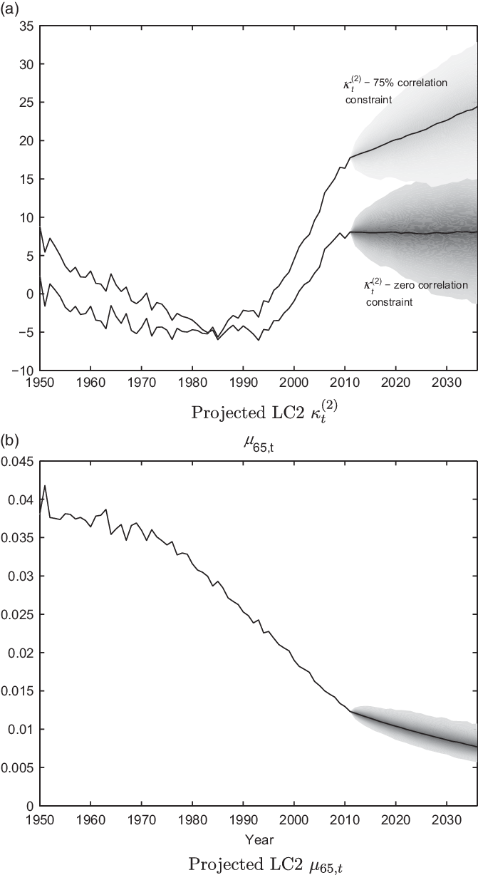
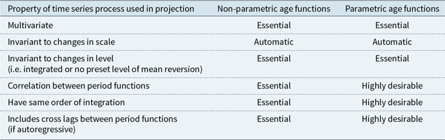
By interpreting the angle between different period functions as their correlation, as discussed in section 2, we also see that the lack of identifiability issues in AP mortality model means that correlations between different period functions are also not meaningful, since they too depend upon the arbitrary identifiability constraints. More generally, the behaviour of any one period function has no objective meaning unless it is also true of any linear combination of all of the period functions. This has important consequences when performing graphical checks on the fitted parameters, and also when we come to project a model, as discussed in section 9.
In the terminology of section 2.2, we see that a general AP model of the form in equation (3) has  $X+N(X+T)$
parameters, i.e., the parameter space has dimension
 $X+N(X+T)$
. However, the invariant transformations in equations (11) and (12) have
 $N(N+1)$
parameters which imply that we need to impose
 $N(N+1)$
identifiability constraints in order to specify a unique set of parameters. This means that the restricted parameter space,
 $\mathcal{P}$
, is an
 $X+N(X+T) - N(N+1)$
dimensional subspace of
 $\mathbb{R}^X \times \mathbb{R}^{NX} \times \mathbb{R}^{NT}$
, and, correspondingly, the model space
 $\mathcal{M}$
is an
 $X+N(X+T) - N(N+1)$
dimensional subspace of
 $\mathbb{R}^{X \times T}$
.
The  $N(N+1)$
constraints imposed will still be arbitrary in the sense that they are entirely the choice of the model user. It is impossible to choose between models with the same structure in equation (1) and the same fitting procedure but different identifiability constraints by statistical methods. However, the different terms in them may have different subjective demographic significance depending upon the identifiability constraints imposed.
5. Identifiability in the LC2 Model
In section 3, we saw how the different identifiability issues were solved in the simplest and most commonly used AP mortality model. We now take the intuition derived from that model and also the theory discussed in section 4 and apply them to the next simplest AP mortality model with non-parametric age functions. The two-term model in Renshaw & Haberman (Reference Renshaw and Haberman2003b) (which we shall refer to as the LC2 model) is usually written as
 \begin{align}\ln(\mu_{x,t}) &= \alpha_x + \beta^{(1)}_x \kappa^{(1)}_t + \beta^{(2)}_x \kappa^{(2)}_t\end{align}
The LC2 model applies the same normalisation scheme to the age functions to set their scale and the same level for the period functions to set their location as in the original LC model. Doing so, however, can lead to identifiability issues in this more complicated model as we now show.
5.1 Location
Because the location of the period functions is not identifiable, Renshaw & Haberman (Reference Renshaw and Haberman2003b) set their level by imposing  $\sum_t \kappa^{(i)}_t = 0$
for
 $i = 1,2$
. As with the LC model, this gives the static age function the demographic significance of representing “average” mortality rates across the period range of the data. This does not cause any additional issues for the LC2 model, so long as it is imposed via an identifiability constraint on
 $\kappa_t$
and not by imposing the form of
 $\alpha_x$
(as discussed in Appendix A).
5.2 Scale
To set the scale of the AP terms, Renshaw & Haberman (Reference Renshaw and Haberman2003b) imposed the constraint  $\sum_x \beta^{(i)}_x\,{=}\,1$
for
 $i = 1,2$
, again, in order to be consistent with the convention established by Lee & Carter (Reference Lee and Carter1992). However, the justification for this normalisation scheme makes most sense under the assumption that
 $\beta^{(i)}_x \geq 0$
for all x – indeed, this is imposed on the LC model in Haberman & Renshaw (Reference Haberman and Renshaw2009) at the expense of goodness of fit to the data. If
 $\beta^{(i)}_x \geq 0$
, then
 $\sum_x \beta^{(i)}_x = 1$
constrains the age function to be in the range [0, 1]. The values of
 $\beta^{(i)}_x$
, therefore, can be felt to represent a proportion of the factor
 $\kappa^{(i)}_t$
impacting mortality at age x. In general, however, it may be the case that
 $\beta^{(i)}_x < 0$
at some ages, especially in models with multiple AP terms. If so, the interpretation of the age functions as measuring the proportion of the change is no longer applicable.
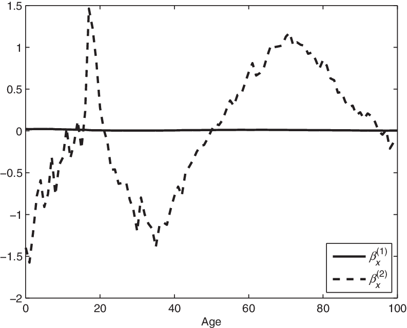
Figure 1 shows the age functions from the LC2 model fitted to data for men in the UKFootnote 12 with the constraint  $\sum_x \beta^{(i)}_x = 1$
for
 $i=1,2$
. We see that if
 $\beta^{(i)}_x \leq 0$
for some x, as is the case for the second age function, then the identifiability constraint on the age function no longer limits it to a particular range of values. Indeed,
 $\beta^{(i)}_{x_1}$
can take arbitrarily high positive values, as long as there exists a correspondingly low
 $\beta^{(i)}_{x_2}$
(i.e. large magnitude and negative) to compensate. This is in contrast to
 $\beta^{(1)}_x$
, which is greater than zero for all ages, and hence is comparatively close to zero across the whole age rangeFootnote 13. This undermines the rationale for selecting a common normalisation scheme for the age functions, which was to aid comparisons of the relative importance of the different AP terms.
LC2 age functions with  $\sum_x \beta^{(i)}_x = 1.$

The identifiability constraint  $\sum_x \beta^{(i)}_x = 1$
can also, theoretically, lead to numerical problems when fitting the model to data. In practice, the constraint is imposed by taking the set of parameters generated by the fitting algorithm (which do not have any identifiability constraints imposed) and using the transformation in equation (8) with
 $b = \sum_x \beta^{(i)}_x$
, i.e.,
 $\hat{\beta}^{(i)}_x = \frac{1}{\sum_\xi \beta^{(i)}_\xi }\beta^{(i)}_x$
. This gives an equivalent set of parameters (with the same fit to the data), but where
 $\sum_x \hat{\beta}^{(i)}_x = 1$
by construction. If, however,
 $\sum_x \beta^{(i)}_x = 0$
for whatever reason, this procedure will fail as applying the transformation involves dividing by zero, even if the age function fitted originally by the algorithm is reasonable. While this is unlikely, it is far more common that we find
 $\sum_x \beta^{(i)}_x \approx 0$
, which will then lead to the revised parameters (with the constraint imposed) being infeasibly large, and which may, in turn, generate problems with the fitting algorithm.
Both of these problems with the normalisation scheme are caused because simple summation over x is not a true norm. A true norm,  $\|v\|$
, for a vector space,
 $\mathcal{V}$
, of a vector, v, is defined by the properties
1.
$\|v \| \geq 0 \; \forall v \in \mathcal{V}$
;2.
$\|v \| = 0 \iff v = 0$
;3.
$\| a v \| = |a| \| v \| \; \forall a \in \mathbb{R}$
; and4.
$\| v_1 + v_2 \| \leq \|v_1\| + \| v_2 \|$
.


These properties mean that we can use a true norm to define distances and scales within the vector space and therefore make them useful when specifying a normalisation scheme. However, since  $\sum_x \beta^{(i)}_x$
is not a true norm in
 $\mathbb{R}^X$
, we are not able to use this normalisation scheme to compare scales for the age functions, and cannot assume that
 $\sum_x \beta^{(i)}_x >0$
in our fitting algorithms when we come to impose the identifiability constraints.
Normalisation schemes using true norms on  $\mathbb{R}^X$
, such as
 $\sum_x |\beta^{(i)}_x| = 1$
or
 $\sum_x (\beta^{(i)}_x)^2 = 1$
, will not suffer from these issues. When it comes to normalising the fitted age function, a procedure using a true norm for the normalisation scheme will never involve division by zero if the transformation in equation (8) is used with any non-trivial age functions. Therefore, in most circumstances, normalisation schemes based on true norms will be preferableFootnote 14.
However, we note that normalisation schemes based on true norms are not perfectly identified, since the transformation
 \begin{align}\{\hat{\beta}^{(i)}_x, \hat{\kappa}^{(i)}_t \} = \{-\beta^{(i)}_x, -\kappa^{(i)}_t\} \end{align}
is an invariant transformation of the parameters where the new parameters still satisfy the identifiability constraints. In principle, we could solve this by choosing alternative sets of normalisation constraints, for instance
 \begin{align*}sign\left(\sum_x \beta^{(i)}_x \right) \sum_x \left( \beta^{(i)}_x \right)^2 = 1\end{align*}
which are still based on using true norms but are not invariant to changing the sign of the age function. However, the specific transformation causing this problem has few practical consequences when fitting the model, since the transformation is not continuous. When fitting the LC or LC2 models using maximum likelihood techniques, for instance, we make small adjustments to the parameters at each iteration and so it is not possible to move smoothly from one set of acceptable parameters to another when fitting the model. In addition, the transformation in equation (14) can be applied to any set of parameters after fitting the model and, hence, can be used to select the sign of the age function based on the judgement of the user when reviewing the fitted parameters.
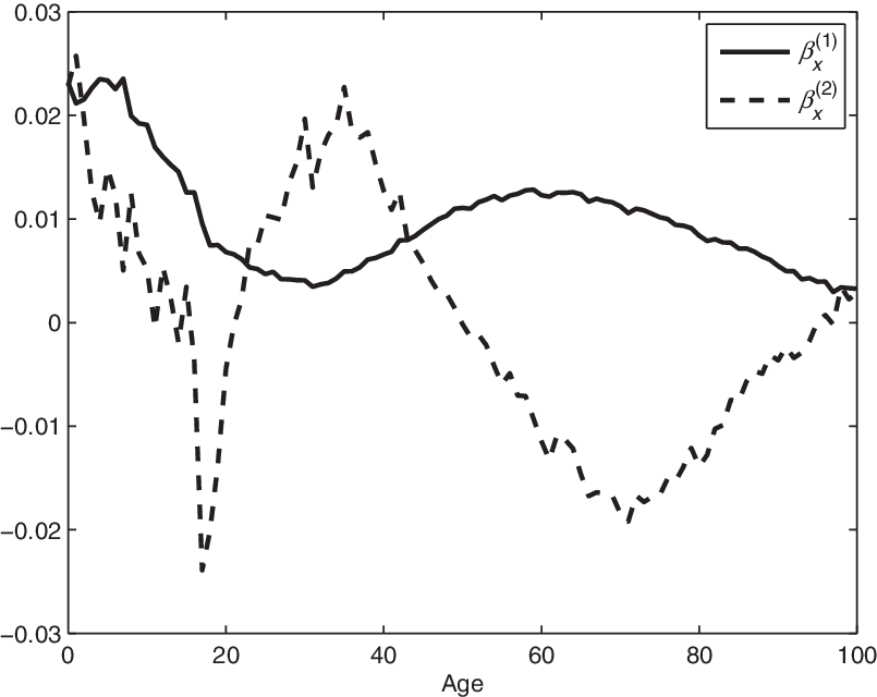
To illustrate this, consider the age functions shown in Figure 2 which fit the LC2 model to the same data as in Figure 1 with the normalisation scheme  $\sum_x |\beta^{(i)}_x| = 1$
. This normalisation scheme gives a model with exactly the same fit to the data, but the estimated parameters for the age and period functions are now of the same order of magnitudeFootnote 15, which may make this model easier to project. We also avoid the possibility of any computational problems when imposing the identifiability constraint, since the divisor,
 $\sum_x |\beta^{(i)}_x|$
, will not be zero for any non-trivial age function.
LC2 age functions with  $\sum_x |\beta^{(i)}_x| = 1.$

5.3 Rotation
We established in section 4 that  $N(N+1)$
constraints were necessary to restrict the parameters in a general AP mortality model with non-parametric age functions, due to the number of free parameters in the transformations in equations (11) and (12). In the context of the LC2 model, this means that we would require six identifiability constraints. However, only four identifiability constraints (two on the level of the two period functions, two on the normalisation of the two age functions) were described in Renshaw & Haberman (Reference Renshaw and Haberman2003b). We, therefore, have an additional two invariant transformations of the parameters which give the same fit to data and which satisfy the constraints already explicitly imposed by Renshaw & Haberman (Reference Renshaw and Haberman2003b). These can be written as
 \begin{align}\begin{pmatrix} \hat{\beta}^{(1)}_x \\[4pt] \hat{\beta}^{(2)}_x \end{pmatrix} &= \left(\begin{array}{c@{\quad}c} \theta & 1-\theta \\[4pt] 0 & 1 \end{array}\right) \begin{pmatrix} \beta^{(1)}_x \\[4pt] \beta^{(2)}_x \end{pmatrix} \notag \\[4pt]\begin{pmatrix} \hat{\kappa}^{(1)}_t \\[4pt] \hat{\kappa}^{(2)}_t \end{pmatrix} &= \frac{1}{\theta} \left(\begin{array}{c@{\quad}c} 1 & \theta-1 \\[4pt] 0 & \theta \end{array}\right)\begin{pmatrix} \kappa^{(1)}_t \\[4pt] \kappa^{(2)}_t \end{pmatrix} \end{align}
and
 \begin{align}\begin{pmatrix} \hat{\beta}^{(1)}_x \\[4pt] \hat{\beta}^{(2)}_x \end{pmatrix} &= \left(\begin{array}{c@{\quad}c} 1 & 0 \\[4pt] 1-\phi & \phi \end{array}\right) \begin{pmatrix} \beta^{(1)}_x \\[4pt] \beta^{(2)}_x \end{pmatrix} \notag \\[4pt]\begin{pmatrix} \hat{\kappa}^{(1)}_t \\[4pt] \hat{\kappa}^{(2)}_t \end{pmatrix} &= \frac{1}{\phi} \left(\begin{array}{c@{\quad}c} \phi & 0 \\[4pt] \phi-1 & 1 \end{array}\right)\begin{pmatrix} \kappa^{(1)}_t \\[4pt] \kappa^{(2)}_t \end{pmatrix}\\[-15pt]\nonumber \end{align}
These transformations can be thought of as “rotations” of the AP functions, because they change the angle between age and period functions, but the normalisation scheme  $\sum_x \hat{\beta}^{(i)}_x = 1$
still holds. They also clearly illustrate that we have an additional two degrees of freedom, given by the free parameters
 $\theta$
and
 $\phi$
, which do not change the fitted mortality rates but which should be used to impose two more identifiability constraints on the model.
This does not necessarily mean that the model in Renshaw & Haberman (Reference Renshaw and Haberman2003b) was poorly identified, however. Although the authors did not explicitly acknowledge the existence of these additional identifiability constraints, their use of singular value decomposition to fit the model imposed them implicitly. By taking singular values (or equivalently, principal components), age and period functions are selected so that  $\sum_t \kappa^{(i)}_t \kappa^{(j)}_t = 0$
and
 $\sum_x \beta^{(i)}_x \beta^{(j)}_x = 0$
for
 $i \neq j$
. We call such age and period functions “orthogonal” to each other as the angle between them defined earlier using the standard inner product will be
 $\frac{\pi}{2}$
. This implicit imposition of additional identifiability constraints leads to a fully identified model.
If alternative fitting methods are used, such as maximum likelihood (e.g. in Brouhns et al. (Reference Brouhns, Denuit and Vermunt2002a)) or minimal deviance (e.g. in Renshaw & Haberman (Reference Renshaw and Haberman2003a)), then these constraints must be imposed explicitly in order to obtain a fully identified model. To impose these orthogonality constraints for a general set of LC2 parameters, we would therefore need to solve  $\sum_t \hat{\kappa}^{(i)}_t \hat{\kappa}^{(j)}_t = 0$
and
 $\sum_x \hat{\beta}^{(i)}_x \hat{\beta}^{(j)}_x = 0$
with the transformed parameters defined by equations (15) and (16) in order to find
 $\theta$
and
 $\phi$
.
We also note the special case where  $A= \left(\begin{array}{c@{\quad}c} 0 & 1 \\[1pt] 1 & 0 \end{array}\right)$
(i.e.
 $\theta = \phi = 1$
when equations (15) and (16) are composed), which relates to the transformation
 \begin{align}\{ \hat{\beta}^{(1)}_x, \hat{\kappa}^{(1)}_t, \hat{\beta}^{(2)}_x, \hat{\kappa}^{(2)}_t \} = \{ \beta^{(2)}_x, \kappa^{(2)}_t, \beta^{(1)}_x, \kappa^{(1)}_t \} \end{align}
This is an invariant transformation of the parameters where the new parameters still satisfy the identifiability constraints. However, it amounts to simply re-labelling the AP terms and arises because the identifiability constraints are the same for all AP terms. Similar to the case in equation (14), this situation could, in principle, be solved by using different identifiability constraints for the different AP terms, for instance
 \begin{align*}\sum_x | \beta^{(1)}_x | = 1 \\\sum_x \left( \beta^{(2)}_x \right)^2 = 1\end{align*}
which breaks the symmetry between the different AP terms and, thus, prevents them being relabelled. However, as with equation (14), the transformation in equation (17) has few practical consequences, since it is not continuous and so it is not possible to move smoothly from one set of acceptable parameters to another when fitting the model. Furthermore, using different identifiability constraints for the different AP terms conflicts with a desire for their scale to be comparable with each other and, hence, we do not believe that this issue is important in practice.
If maximum likelihood methods are used to estimate the parameters in a model, it is useful that these estimators are independent of each other. This helps to give more efficient fitting algorithms for estimation and is also useful when allowing for parameter uncertainty using the technique of Brouhns et al. (Reference Brouhns, Denuit and Vermunt2002b) discussed in section 8. Assuming the canonical link function is used as discussed in Hunt & Blake (Reference Hunt and Blake2020b), the independence of the estimators can be assessed by consideration of the information matrix for the different parameters
 \begin{align*}I(\beta^{(i)}_x, \beta^{(j)}_x) &= \mathbb{E}\left[\frac{\partial^2 \mathcal{L}}{\partial \beta^{(i)}_x \partial \beta^{(j)}_x} \right] \\[3pt]&= - \sum_t \mathbb{V}ar(D_{x,t}) \kappa^{(i)}_t \kappa^{(j)}_t \\[3pt]I(\kappa^{(i)}_t, \kappa^{(j)}_t) &= \mathbb{E}\left[\frac{\partial^2 \mathcal{L}}{\partial \kappa^{(i)}_t \partial \kappa^{(j)}_t} \right] \\[3pt]&= - \sum_x \mathbb{V}ar(D_{x,t}) \beta^{(i)}_x \beta^{(j)}_x\end{align*}
Therefore, we see that orthogonal age and period functions are independent of each other if  $\mathbb{V}ar(D_{x,t})$
is constant across ages and years. This assumption is implicitly made when using singular value decomposition or principal components analysis to estimate parameters. However, the assumption is not consistent with the use of the Poisson or binomial distribution for death counts, as discussed in Hunt & Blake (Reference Hunt and Blake2020b). Under these distributions, the variance of death counts depends upon the exposure to risk at different ages, which changes considerably over different ages and years and is more realistic in practice.
In principle, we could impose independent parameter estimates using the transformations in equations (15) and (16) with carefully selected values of  $\theta$
and
 $\phi$
to obtain an equivalent set of parameters. Doing so would simply be choosing an alternative (but equally valid) set of identifiability constraints. However, in practice, this would mean constraints that are both more difficult to impose than the traditional orthogonality constraints using the Euclidean inner product, and which lose the connection between the inner product and the sample moments of
 $\kappa^{(i)}_t$
. In practice, imposing
 $\sum_t \kappa^{(i)}_t \kappa^{(j)}_t = 0$
and
 $\sum_x \beta^{(i)}_x \beta^{(j)}_x = 0$
for
 $i \neq j$
to obtain orthogonal age and period functions is a convenient and useful set of identifiability constraints.
Whichever set of constraints is imposed on the angles between different period functions, the most important thing is, however, to impose some form of constraint. A failure to do so may result in the fitting routine failing to converge or, alternatively, the fitting routine may give model parameters which depend upon the initial parameter estimates used in the algorithm. Similarly, the angles between different age functions must also be constrained in order to fully identify the model. This has implications for estimated parameter uncertainty, as discussed in section 8.
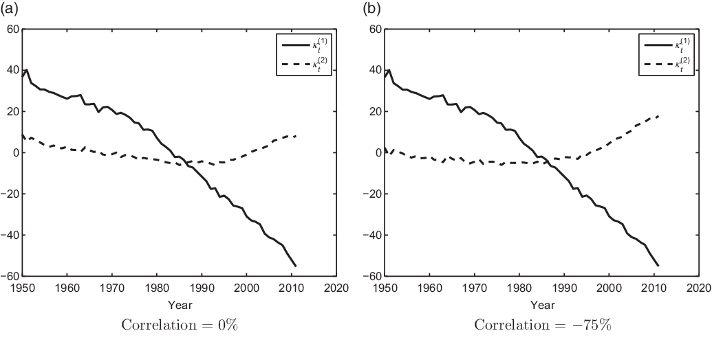
We noted in section 2 that the correlation between two different period functions depends on the angle between them. This means that we see that the correlations we find between period functions from our fitted parameters depends only on the identifiability constraints chosen, and so are not meaningful. For instance, the constraint  $\sum_t \kappa^{(i)}_t \kappa^{(j)}_t = 0$
imposes independence on the period functions over the historical range of the data when they are considered as time series. Figure 3 shows period functions for the LC2 model fitted to the same data as above, but with two different constraints on the angles between them. In Figure 3(a), the period functions are orthogonal whereas, in Figure 3(b), they have a correlation of 75%Footnote 16. However, both sets of parameters give identical fits to the historical data. This will have important consequences when we come to project the model in section 9.
Period functions from the LC2 model.

In situations such as Renshaw & Haberman (Reference Renshaw and Haberman2003b), where orthogonality constraints on the AP terms have been imposed implicitly by the fitting mechanism, we believe that it is important to recognise and state them clearly. Not only will this clarify which features of graphs of the age and period terms are meaningful but it also ensures that we assess the dimension of  $\mathcal{P}$
(i.e. the number of degrees of freedom in the model) correctly. This is important when assessing the goodness of fit for the model.
As an example of this, in Haberman & Renshaw (Reference Haberman and Renshaw2011), the LC2 model is compared against other mortality models using various measures including the Akaike Information Criterion, Bayes Information Criterion and Hannan-Quinn Criterion. All of these measures use the number of degrees of freedom (i.e.  $dim(\mathcal{P}$
)) of the model to penalise the log-likelihood. By failing to explicitly state the orthogonality constraints placed on the AP terms in the LC2 model and, therefore, failing to include them in the count of restrictions placed upon the model parameters, the study overestimates the number of degrees of freedom in the model. This excessively penalises the LC2 model relative to its comparators.
Using the invariant transformations to impose orthogonality on the age and period functions generalises naturally to more complicated models with  $N > 2$
. Identifiability in-sample in a model with non-parametric AP terms is therefore not problematic if fitting methods based on singular value decomposition or principal component analysis are used (except for setting the locations of the
 $\kappa^{(i)}_t$
and the scale for the
 $\beta^{(i)}_x$
by imposing an appropriate normalisation scheme).
6. Identifiability in Models with Parametric Age Functions
In contrast to the non-parametric age functions considered above, we define a “parametric” age function to be one which takes a specific functional form that is defined by an algebraic formula, i.e.,  $\beta^{(i)}_x = f^{(i)}(x;\,\theta^{(i)})$
Footnote 17. In order to specify a mortality model with parametric age functions, we need to define these formulae. Mathematically, AP mortality models with parametric age functions are similar to their non-parametric counterparts, except that the age functions are fixed or selected from a family with a small number of free parameters rather than being allowed to vary freely across
 $\mathbb{R}^X$
. This has important consequences for the identifiability issues in the model.
To illustrate, let us consider the following two pedagogical mortality models
 \begin{align}\eta_{x,t} &= \alpha_x + \kappa^{(1)}_t + (x-\bar{x}) \kappa^{(2)}_t \end{align}
 \begin{align}\eta_{x,t} &= \alpha_x + \kappa^{(1)}_t + e^{-\lambda x} \kappa^{(2)}_t \quad\end{align}
where  $\bar{x} =0.5(X+1)$
. The first of these is similar to the widely used Cairns-Blake-Dowd (CBD) model of Cairns et al. (Reference Cairns, Blake and Dowd2006a), but with the inclusion of an explicit static age function, and therefore we refer to it as the CBDX model. The second model, which we refer to as the exponential model, uses an exponentially decreasing function of age as the second age function, with the parameter
 $\lambda$
being a free parameter of the model determined by the data. Such a model has not been proposed to date, but similar terms have been used within the “general procedure” of Hunt & Blake (Reference Hunt and Blake2014).
We say that the formulae used for the age functions in equations (18) and (19) “define” these models. Different definitions for the age functions give different models. However, we also define the concept of “equivalence” between models with parametric age functions. Two models are equivalent in this sense if they have different definitions for the age functions, but still give the same fitted mortality rates and hence the same fit to data.
We note that the CBDX model is linear in its parameters, and so can be fitted using generalised linear models, as discussed in McCullagh & Nelder (Reference McCullagh and Nelder1983) and Currie (Reference Currie2014). However, since  $\lambda$
is a free parameter of the model, the second AP term in the exponential model is non-linear in the sense of McCullagh & Nelder (Reference McCullagh and Nelder1983), Chapter 11, and so more complicated methods for fitting the model are necessary. Therefore, using parametric age functions is not equivalent to using a linear model except in a few simple cases. We will see below that it is these non-linear cases which tend to have more complicated identifiability issues.
Mathematically, we can see that both models in equations (18) and (19) are similar to the LC2 model, but with specific parametric functions for  $\beta^{(1)}_x$
and
 $\beta^{(2)}_x$
. One might be tempted to believe that they have exactly the same identifiability issues as those in the LC2 model discussed in section 5. However, the imposition of specific functional forms for the age functions has changed whether the invariant transformations of the LC2 model can be applied in practice.
Because the form of the age functions defines the model being used, these forms cannot change under invariant transformations, otherwise we would obtain a different model. Therefore, we require that any invariant transformations of the model also leave the age functions unchanged, i.e.,  $\hat{f}^{(i)}(x;\,\theta^{(i)}) = f^{(i)}(x;\,\theta^{(i)})$
. This restriction reduces the number of invariant transformations, and therefore the number of identifiability constraints which need to be imposed when fitting the model to data. We discuss the implications of this on the different identifiability issues below.
6.1 Location
We noted in section 4 that the transformation in equation (12) does not change the form of the age functions. Accordingly, it can still be applied to change the levels of the period parameters in exactly the same manner as described in section 4, whilst leaving the fitted mortality rates and the functional forms of the age functions unchanged. The period functions in models with parametric age functions therefore still have unidentified locations, and so we still need to impose levels on the period parameters in exactly the same manner as we did in section 5. Most users of such models impose  $\sum_t \kappa^{(i)}_t = 0$
, consistent with the choice made for models with non-parametric age functions and with a similar interpretation. However, for models which have a specific form of the static age function imposed a priori, this is not necessary, as discussed in Appendix A.
6.2 Scale
We see that the transformation in equation (11) takes linear combinations of the old age and period functions in order to create new AP terms. Therefore, these transformations will change the form of the age functions in a model with parametric age functions. Since the form of the age functions defines the model being used, the transformations in equation (11) cannot be used in models with parametric age functions.
In section 5, we saw that these transformations were useful in models with non-parametric age functions when it came to imposing a normalisation scheme on the age functions and orthogonalising them with respect to each other. This was beneficial as it enabled comparability and near-independence between different AP terms. It is therefore desirable to also achieve the same properties for models with parametric age functions.
We also see that although using the transformations in equation (11) in models with parametric age functions gives different age functions (and therefore different models), they do not affect the fitted mortality rates: all the models obtained by using these transformations are equivalent in the sense defined above. It therefore makes sense to choose, from the set of models equivalent to the one we are interested in, a model with age functions which have the desirable properties of possessing a standard normalisation scheme and being orthogonal. We discuss how this can be done in this section and section 6.3, respectively.
Most mortality models with parametric age functions have the age functions defined in their simplest and most natural form. However, choosing definitions for their simplicity rather than for desirable statistical properties, such as having a common normalisation scheme, can lead to issues when comparing age and period terms within the same model and between different models. We show this below for the CBDX and exponential models in equations (18) and (19), respectively. However, for each of these models, we also show how this issue can be resolved by using alternative definitions of the age functions to give models which have far more comparable age and period terms.
First, let us consider how a common normalisation scheme for the age functions can be achieved in the CBDX model in equation (18). In the LC2 model, Renshaw & Haberman (Reference Renshaw and Haberman2003b) imposed the normalisation scheme  $\sum_x \beta^{(i)}_x = 1$
on the age functions in the model, using the transformations in equation (11). In contrast, the age functions in equation (18) already have defined scales, i.e.,
 $\sum_x\, f^{(1)}(x) = \sum_x 1 = X$
and
 $\sum_x\, f^{(2)}(x) = \sum_x (x-\bar{x}) = 0$
.
However, these defined scales cause problems when it comes to comparing the AP terms. The most important of these issues is that the scale of  $f^{(2)}(x)$
is zero, which is not sensible for a functions which is not identically equal to zero. This is a consequence of using a normalisation scheme which is not based on using a true norm. In section 5, we saw that a more sensible choice of normalisation scheme was to use
 $\sum_x |\beta^{(i)}_x|$
to define the scales of the age functions. Using this for the CBDX model, we find
 $\sum_x |\,f^{(1)}(x)| = \sum_x 1 = X$
and
 $\sum_x |\,f^{(2)}(x) |= \sum_x |(x-\bar{x})| = 0.25X^2$
if X is even or
 $0.25(X-1)(X+1)$
if X is odd.
However, this fails to resolve the second problem, which is that different scales are defined for each of the AP terms, i.e., the scale of the first age function is proportional to the number of ages, X, whilst the scale of the second in proportional to  $X^2$
. This makes comparisons difficult, both between the CBDX and LC2 models and between the first and second AP terms within the CBDX model. The differing scales of the corresponding period functions can also lead to numerical problems when we try to project them using multivariate methods, as discussed in section 9.
To ensure that the age functions have the same scale, we need to define a model equivalent to that in equation (18) where the age functions have this property. Trivially, we see that the model
 \begin{align}\eta_{x,t} &= \alpha_x + \frac{1}{X}\kappa^{(1)}_t + \frac{4(x-\bar{x})}{X^2} \kappa^{(2)}_t \end{align}
(assuming X is even) is equivalent to the model in equation (18)Footnote 18. All that differs between the models in equations (18) and (20) is the precise definition of the age functions, although the age functions in both models have the same functional form (i.e. a constant and a linear function of age, x). In addition, we see that in the model in equation (20),  $\sum_x |\,f^{(i)}(x) |= 1$
for both age functions. In particular, this has the advantage of greater comparability between the AP terms.
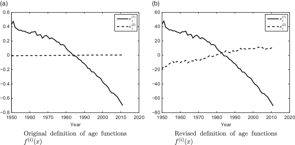
To illustrate the impact of ensuring that the age functions have a common normalisation scheme, Figure 4 shows the period functions from the two CBDX models in equations (18) and (20), fitted to the same data as used for the LC2 model in section 5, with both the original and the revised normalisation schemes. We see that the magnitude of the different period functions fitted with the original model in equation (18) differs enormouslyFootnote 19. This can be a problem as most numerical algorithms for analysing time series are optimised to work best on series of comparable orders of magnitude. In contrast, the revised CBDX model in equation (20) gives period functions of comparable magnitudeFootnote 20. The common scale also means that it is easier to compare these period functions with those in Figure 3 from the LC2 model.
Period functions from the CBDX model.

Turning now to the exponential model in equation (19), we find similar issues for the normalisation scheme of the age functions. In the exponential model,  $\sum_x |\,f^{(1)}(x)| = X$
as before for the CBDX model, which can be dealt with in exactly the same manner. In addition,
 $\sum_x |\,f^{(2)}(x;\,\lambda)| = \sum_x e^{-\lambda x} = \frac{e^{-\lambda}(1-e^{-\lambda (X+1)})}{ 1-e^{-\lambda}} \approx \frac{e^{-\lambda}}{1-e^{-\lambda}}$
for the second age function. Not only will this be different from the scale of the first AP term, but the scale is a function of the free parameter
 $\lambda$
. Since
 $\lambda$
varies during the fitting process, this will alter the scale of
 $f^{(2)}(x;\,\lambda)$
. Hence,
 $\lambda$
will be trying to fulfil two purposes simultaneously: first, describing the shape of the age function and second, determining its scale, i.e., the relative importance of the AP term. This confusion of different purposes can cause numerical instability in most fitting algorithms, which may be one reason why age functions with free parameters have not been commonly used in practice.
For the CBDX model, we obtained a common normalisation scheme for the age functions by choosing slightly different definitions for the age functions, i.e., we defined alternative age functions which were equal to the original ones, but rescaled by  $\sum_x |\,f^{(i)}(x)|$
. For the exponential model, we do the same thing, to obtain
 \begin{align}\eta_{x,t} &= \alpha_x + \frac{1}{X}\kappa^{(1)}_t + \frac{ 1-e^{-\lambda}}{e^{-\lambda}(1-e^{-\lambda (X+1)})} e^{-\lambda x} \kappa^{(2)}_t \end{align}
The only difference in this case is that the second age function is rescaled by a function of the free parameter,  $\lambda$
, rather than a constant in the case of the CBDX model. Again, we see that the age functions have the same functional forms (a constant and an exponential function of age) as before, but with the normalisation scheme
 $\sum_x |\,f^{(2)}(x;\,\lambda)| = 1 \; \forall \lambda$
as
 $\lambda$
is varied when fitting the model. This contrasts with the model in equation (19) and ensures that both age functions have the same normalisation scheme and so are more comparable.
We call age functions such as the revised  $f^{(2)}(x;\,\lambda)$
in equation (21) “self-normalising”, as they have the property that our desired normalisation scheme is imposed automatically for all values of the free parameters in the age function (i.e.
 $\sum_x |\,f^{(i)}(x;\, \theta^{(i)})| = 1 \; \forall \theta^{(i)}$
). Self-normalisation is an important and useful property. Most importantly, the common normalisation scheme allows for comparability between different age functions (potentially with very different functional forms) in a model, independent of their shape. Furthermore, by allowing the value of the free parameter to describe the shape of the age function, without impacting the scale of the AP term, we find that self-normalising age functions are considerably more robust (in the sense of being likely to converge) and stable to small changes in the data. For this reason, the age functions used in the “toolkit” in the Appendix of Hunt & Blake (Reference Hunt and Blake2014) are all self-normalising with respect to the normalisation scheme
 $|\,f^{(i)}(x;\,\theta^{(i)})|\,{=}\,1$
Footnote 21. However, the trade-off is that the numerical routines are significantly more complicated to implement and may need to be written specially for the specific circumstances, rather than adapted from “off-the-shelf” statistical packagesFootnote 22.
In summary, we see that, when the age functions in a mortality model are defined parametrically, a common normalisation scheme for all of them can be achieved by defining the age functions carefully. For more sophisticated age functions involving free parameters estimated from the data, this means defining age functions which are self-normalising, so that the normalisation scheme holds for all values of these parameters as they are varied during the fitting procedure.
6.3 Rotation
In section 6.2, we saw that for models with parametric age functions, we could ensure that the age functions had the same normalisation scheme by carefully defining them to have this property when we specified the model. The same is also true if we want our age functions to be orthogonal to each other.
Again, similar to section 6.2, we start from the fact that most mortality models have their age functions defined in the simplest form, such as in equations (18) and (19). These simple forms are not, necessarily, orthogonal. However, we can define equivalent models where the age functions are orthogonal. Unlike the case of ensuring a common normalisation scheme, however, we will see that orthogonality between age functions is not always a desirable property and may conflict with other desirable properties, such as the terms in the model having distinct demographic significance. Therefore, the choice of whether to define orthogonal age functions or not will depend upon the model in question and the aims of the model user.
For example, consider the CBDX model of equation (18) before normalisation. The model already has orthogonal age functions, since  $\sum_x\, f^{(1)}(x) f^{(2)}(x) = \sum_x (x-\bar{x}) = 0$
. However, we could also consider an equivalent model, with simpler definitions of the age functions of the form
 \begin{align}\eta_{x,t} &= \alpha_x + \kappa^{(1)}_t + x \kappa^{(2)}_t \end{align}
This model is more similar to the form of the original CBD model proposed in Cairns et al. (Reference Cairns, Blake and Dowd2006a). However, we observe that the age functions are not orthogonal, i.e.,  $\sum_x\, f^{(1)}(x) f^{(2)}(x) = \sum_x x= \frac{1}{2}X(X+1)$
. It is easy to see that models in equations (18) and (22) are equivalent, in that they give the same fitted mortality rates and are linked through a transformation of the form in equation (11). The form of the age functions in equation (18) was introduced in Cairns et al. (Reference Cairns, Blake, Dowd, Coughlan, Epstein, Ong and Balevich2009) and, in practice, has proved far more popular than the simpler age functions in equation (22), in part because it is more robust to fit to data due to the parameter estimates for the period functions being nearly independent of each other. Consequently, we see that defining orthogonal age functions can be desirable, even if it comes at the expense of a slightly more complicated definition of the age functions.
The age functions in the CBDX model are of constant and linear form, i.e., polynomials of order zero and one, respectively. Defining orthogonal age functions, as in equation (18), has not changed this form, merely selected the first two members of the orthogonal family of polynomials, i.e., the Legendre polynomialsFootnote 23. The orthogonal age functions in equation (18) have the same demographic significance as the simpler age functions in equation (22), but the additional desirable property of orthogonality. Generalising this, we see that choosing orthogonal age functions does not change their form and hence does not affect their demographic significance when the age functions come from the same functional family (e.g. polynomials).
However, this is not the case when the age functions come from different functional families. We see this by considering the exponential model once more. To define orthogonal age functions for this model, we could select a model equivalent to that in equation (19) with orthogonal age functions, namely,
 \begin{align*}f^{(2)}(x;\,\lambda) &= e^{-\lambda x} - \frac{e^{-\lambda}(1-e^{-\lambda (X+1)})}{ 1-e^{-\lambda}}\end{align*}
We see that the age functions in this model are orthogonal as  $\sum_x\, f^{(1)}(x) f^{(2)}(x;\,\lambda) = 0 \; \forall \lambda$
. This revised model is equivalent to that in equation (19), as it gives the same fitted mortality rates and the two models are linked by a transformation of the form of that in equation (11).
However, it is likely that we originally selected an exponential function for its demographic significance (e.g. a mortality effect which decreases rapidly with age, such as that associated with the relatively high rate of infant mortality). The redefined  $f^{(2)}(x;\,\lambda)$
will not possess this demographic significance, as it will start positive and then tend rapidly to a negative constant. This lack of demographic significance is unlikely to be desirable. Therefore, orthogonal age functions can conflict with a desire for each AP term to have distinct demographic significance for models with parametric age functions coming from different functional families.
In summary, we find that orthogonality between age functions makes most sense when the age functions come from the same family, such as polynomials, and therefore can be orthogonalised easily. For models with very different functional forms for the age functions, orthogonalisation is unlikely to be desirable as it will conflict with a desire to give each AP term distinct demographic significance.
7. Identifiability in Mixed Models
Some AP mortality models have mixed parametric and non-parametric age functions, such as the model of Wilmoth (Reference Wilmoth1990) (excluding the cohort term) and the models used to explore the data in Hunt & Blake (Reference Hunt and Blake2014). Other studies, such as Reichmuth & Sarferaz (Reference Reichmuth and Sarferaz2008), have proposed extending the LC model with exogenous variables, such as economic or health indicators, which take the form of period functions with a prescribed form. The identifiability issues in such mixed models, however, are similar to those addressed in sections 4 and 5 above.
As with models with purely parametric age functions, in mixed models, the prescribed form of the age or period functions means that we must restrict the transformations in equations (11) and (12) so that they remain unchanged. For instance, consider the model
 \begin{align}\eta_{x,t} &= \alpha_x + f(x) \kappa^{(1)}_t + \beta_x \kappa^{(2)}_t \end{align}
This model has one parametric age function, f(x), and one non-parametric age function,  $\beta_x$
, while the two period functions are freely varying. We see that the transformation in equation (12) is still applicable, as it will not change the form of f(x) and therefore we still need to define the location of the period functions via an identifiability constraint.
However, we see that the transformation
 \begin{align}\{ \hat{f}(x), \hat{\kappa}^{(1)}_t, \hat{\beta}_x, \hat{\kappa}^{(2)}_t\} = \left\lbrace f(x), \kappa^{(1)}_t + ab\kappa^{(2)}_t, \frac{1}{a} \beta_x - b f(x), a \kappa^{(2)}_t \right\rbrace\end{align}
is an invariant transformation of the model in equation (23) and avoids changing the form of f(x). This is a special case of the general transformation in equation (11), with the matrix, A, taking the restricted form  $A = \left(\begin{array}{c@{\quad}c} 1 & ab \\ 0 & a \end{array}\right)$
. We can see that this transformation corresponds to a reduced set of invariant transformations compared with the LC2 model, since it only has two degrees of freedom, compared with the four in the unrestricted matrix, A.
The form of the restrictions on A means that only the scale of  $\beta_x$
(set by a) and the angle between
 $\beta_x$
and f(x) (set by b) are undefined. In such a model, it therefore makes sense to impose a standard normalisation scheme on
 $\beta_x$
, for example,
 $\sum_x |\beta_x| = 1$
, and an orthogonality constraint between
 $\beta_x$
and f(x), i.e.,
 $\sum_x \beta_x\, f(x) = 0$
.
Next, consider the alternative model
 \begin{align}\eta_{x,t} &= \alpha_x + \beta^{(1)}_x K(t) + \beta^{(2)}_x \kappa_t \end{align}
where K(t) is either a deterministic function, such as in Callot et al. (Reference Callot, Haldrup and Lamb2014), or an exogenous variable such as real GDP or an indicator variable to account for an epidemic, such as in Liu & Li (Reference Liu and Li2015), or a war. We also note that this type of model is common in multi-population models where the period function in one population is required to be the same as that in another, for instance, those of Carter & Lee (Reference Carter and Lee1992) and Li & Lee (Reference Li and Lee2005). In this case, we see that we can no longer use the unrestricted transformation in equation (12), since the location of K(t) is set a priori. Therefore, we only need to impose a constraint on the level of the remaining period function, such as  $\sum_t \kappa_t = 0$
.
As with the model in equation (23), we also have a restricted set of transformations of the form in equation (11) in order to avoid changing K(t) in the transformation. In this case, the transformation of the parameters is
 \begin{align}\{ \hat{\beta}^{(1)}_x, \hat{K}(t), \hat{\beta}^{(2)}_x, \hat{\kappa}_t\} = \left\lbrace \beta^{(1)}_x + \frac{b}{a} \beta^{(2)}_x, K(t), \frac{1}{a}\beta^{(2)}_x, a\kappa_t - bK(t)\right\rbrace\end{align}
which leaves K(t) unchanged. In this case, the restricted form of the matrix, A, in equation (11) is  $A = \begin{pmatrix} 1 & 0 \\ -b & a \end{pmatrix}$
, which can be compared to the restricted form for the model in equation (23).
Similarly, these restricted transformations mean that only the scale of  $\beta^{(2)}_x$
(set by a) and the angle between K(t) and
 $\kappa_t$
(set by b) are undefined. Consequently, this transformation can be used to impose a normalisation scheme on
 $\beta^{(2)}_x$
and orthogonalise K(t) and
 $\kappa_t$
by means of additional identifiability constraints. In this case, the orthogonalisation of the period functions has the clear interpretation that
 $\kappa_t$
explains that part of the variation that is independent of the factor K(t). However, this was not done in Liu & Li (Reference Liu and Li2015), which, in the context of that study, made it difficult to interpret the meaning of
 $\kappa_t$
for years when there was an epidemic.
Hence, we see that mixed models act to impose restrictions on the more general set of invariant transformations present in a model with fully non-parametric age functions. These restrictions are specific to different models and depend upon the specification of the model in question. This is especially common in many multi-population mortality models, such as some of those discussed in Villegas & Haberman (Reference Villegas and Haberman2014), which can be interpreted as mixed models where the form of different age and period functions is common to different populations and hence restricted. Consequently, we must analyse each individual model in order to determine which identifiability issues it possesses and, hence, a suitable set of identifiability constraints to impose.
8. Parameter Uncertainty and Hypothesis Testing
8.1 Parameter uncertainty
Having obtained a set of parameters by fitting a model to data with some set of arbitrary identifiability constraints, it is common to investigate the degree of uncertainty associated with these estimated parameters. A number of techniques have been developed to do this, for instance
using the asymptotic normality of parameters estimated by maximum likelihood methods, as in Brouhns et al. (Reference Brouhns, Denuit and Vermunt2002b);
using a “semi-parametric” bootstrap based on Poisson (or binomial) death counts, as in Brouhns et al. (Reference Brouhns, Denuit and Van Keilegom2005);
using a residual bootstrapping method, such as that developed in Koissi et al. (Reference Koissi, Shapiro and Hognas2006) or the more complicated techniques discussed in D’Amato et al. (Reference D’Amato, Lorenzo, Haberman, Russolillo and Sibillo2011) and Debón et al. (Reference Debón, Montes, Mateu, Porcu and Bevilacqua2008), (Reference Debón, Martinez-Ruiz, Montes, Martínez-Ruiz and Montes2010), and
using Bayesian Markov chain Monte Carlo (MCMC) methods, as in Czado et al. (Reference Czado, Delwarde and Denuit2005).
All of these techniques were developed for the LC model, as the simplest and most widely used mortality model. In the following section, we follow this convention and implicitly assume that we are dealing with the LC model. However, in principle, they could all be used with any other AP mortality model.
The first three of these methods have been tested and compared in Renshaw & Haberman (Reference Renshaw and Haberman2008) and all four were compared in Li (Reference Li2014). It is important that any conclusions drawn from them do not depend upon the arbitrary identifiability constraints imposed in the model. Since the fitted mortality rates do not change under the invariant transformations of the model, their variability due to parameter uncertainty should not depend on the identifiability constraints imposed either. Appropriate methods for determining parameter uncertainty should ensure this. Two users of a mortality model, using the same data and method for investigating parameter uncertainty, but using different (but equally valid) identifiability constraints should find the same degree of variability of mortality rates under parameter uncertainty.
It is therefore desirable to start from the difference between the observed and fitted mortality rates, since this will be independent of the identifiability constraints chosen from them model and ensure that our results are consistent with observations. For instance, in Brouhns et al. (Reference Brouhns, Denuit and Van Keilegom2005), Poisson-distributed random death counts were generated at each age and yearFootnote 24. The distribution of the bootstrapped death counts is therefore unaffected by which identifiability constraints are imposed. Likewise, the fitting residuals used in Koissi et al. (Reference Koissi, Shapiro and Hognas2006) depend only on the actual and fitted death counts and thus not on the identifiability constraints used in fitting the model. Therefore, estimates of the impact of parameter uncertainty on observable quantities, such as fitted mortality rates or life expectancies, will be independent of the arbitrary identifiability constraints.
However, estimates for the variability of the model parameters will still only be valid conditional on the chosen set of identifiability constraints. For instance, imposing the constraint  $\kappa^{(i)}_1 = 0$
in a model will mean that
 $\kappa^{(i)}_1$
will trivially not show any variability using the Brouhns et al. (Reference Brouhns, Denuit and Van Keilegom2005) or Koissi et al. (Reference Koissi, Shapiro and Hognas2006) methods, but this will not be the case for other choices of constraints. Therefore, the observed parameter uncertainty should be seen only in the context of the identifiability constraints applied.
It is also important to ensure that the model is fully identified when using these bootstrapping approaches. If the model is not fully identified, we may observe spurious variation in the parameters which does not lead to real variability in the fitted mortality rates. This is of most practical relevance with the orthogonality constraints for models such as the LC2 model in equation (13), as these are often overlooked if maximum likelihood or minimum deviance techniques are used to fit the model.
The alternative approach to starting from the difference between observed and expected mortality rates is to consider the distribution of the model parameters directly. However, methods which generate new samples of parameters directly, such as the asymptotic method of Brouhns et al. (Reference Brouhns, Denuit and Vermunt2002b) or the Bayesian techniques of Czado et al. (Reference Czado, Delwarde and Denuit2005), must be used with considerably more care.
First, consider the asymptotic method of Brouhns et al. (Reference Brouhns, Denuit and Vermunt2002b). This assumes that the variation of the maximum likelihood parameters is given by the information matrix (i.e. the second derivative of the log-likelihood,  $\mathcal{L}$
, with respect to the model parameters evaluated at the selected parameter estimates). The first thing to note here is that, in order to identify the model, the likelihood being maximised is the constrained likelihood. Starting from the forms of the likelihood function in Hunt & Blake (Reference Hunt and Blake2020b), this means that we use Lagrangian multipliers to impose the constraints. For example, to impose the Lee & Carter (Reference Lee and Carter1992) model constraints involves adjusting the likelihood function by
 \begin{align*}\mathcal{L}(d_{x,t};\,\{\alpha,\beta,\kappa\}) &\to \mathcal{L}(d_{x,t};\,\{\alpha,\beta,\kappa\}) - \lambda_1 \sum_t \kappa_t - \lambda_2 \left(1-\sum_x \beta_x\right)\end{align*}
Therefore, the information matrix is explicitly dependent upon the identifiability constraints imposed. For instance, we can see this by considering the second derivative of the likelihood with respect to the age function  $\beta_x$
 \begin{align*}\frac{\partial^2 \mathcal{L}}{\partial (\beta_x)^2} &= -\sum_t \mathbb{V}ar(D_{x,t}) (\kappa_t)^2\end{align*}
if we use the canonical link function, as discussed in Hunt & Blake (Reference Hunt and Blake2020b). If we apply the transformation in equation (9),  $\beta_x$
is unchanged. However, we have
 \begin{align*}\frac{\partial^2 \mathcal{L}}{\partial (\hat{\beta}_x)^2} &= -\sum_t \mathbb{V}ar(D_{x,t}) (\hat{\kappa}_t)^2 \\&= -\sum_t \mathbb{V}ar(D_{x,t}) (\kappa_t + b)^2 \\&= \frac{\partial^2 \mathcal{L}}{\partial (\beta_x)^2} +2b\sum_t \mathbb{V}ar(D_{x,t})\kappa_t - b^2 \sum_t \mathbb{V}ar(D_{x,t})\end{align*}
In this case, the form of the information matrix with respect to  $\beta_x$
has changed under a transformation which did not change
 $\beta_x$
itself. This needs to be taken into consideration carefully and may explain the variation in the uncertainty in the fitted mortality rates observed in Renshaw & Haberman (Reference Renshaw and Haberman2008) when the identifiability constraints are altered.
Next, we consider Bayesian techniques, such as MCMC. As discussed in Nielsen & Nielsen (Reference Nielsen and Nielsen2014), these can often appear to solve identifiability issues but in fact confuse and disguise them. The use of Bayesian methods often involves consideration of the posterior distribution,  $\pi$
, of the parameters given by
 \begin{align*}\ln(\pi(\{\alpha,\beta,\kappa\})) &= \mathcal{L}(d_{x,t};\,\{\alpha,\beta,\kappa\}) + \ln(\phi(\{\alpha,\beta,\kappa\})) + \text{constant}\end{align*}
where  $\phi$
is the prior distribution for the parameters. The log-likelihood function,
 $\mathcal{L}(d_{x,t};\,\{\alpha,\beta,\kappa\})$
, is unchanged by the invariant transformations of the model parameters and so does not depend upon the chosen identifiability constraints. However, in general, the prior distribution
 $\phi$
will change under these transformations, unless it is very carefully chosen. This, in turn, means that the posterior distribution will also vary under the invariant transformations of the model, and so will depend implicitly on any identifiability constraints imposed.
A poorly chosen set of priors implicitly imposes a set of identifiability constraints upon the model. For example, a prior distribution that assumes  $\kappa^{(i)}_t$
follows an AR(1) process around zero implicitly imposes a level on the period parameters. These implicit constraints may conflict with the explicit constraints subsequently imposed (such as a subsequent choice of the level of
 $\kappa^{(i)}_t$
). Even when there are no conflicts, this implicit selection of identifiability constraints is opaque, and it is not clear which features of the posterior distribution are meaningful and which are mere artefacts of the identifiability scheme implicit in the prior.
We therefore recommend that the prior distribution of the model parameters,  $\phi$
, is selected so that it is unchanged by the invariant transformations of the model. This enables a single set of identifiability constraints to be imposed upon the model without internal conflicts, with these constraints being clear and transparent to all other model users, and with the posterior distribution being independent of the arbitrary choice of identifiability constraints (just as the likelihood is).
8.2 Hypothesis testing
Identifiability issues also have important consequences if hypothesis testing on the parameters is performed. In general, hypotheses cannot be tested on the parameter values directly, since they depend upon the identifiability constraints. For instance, testing the hypothesis  $\kappa_T = 0$
in the LC model is meaningless, since we can impose
 $\kappa_T = 0$
(or any other value) by our choice of identifiability constraint. We might be tempted to find combinations of the parameters which are invariant to the transformations of the parameters and test hypotheses based on these. For instance, we may wish to test the hypothesis that mortality is declining faster at age
 $x_1$
than at age
 $x_2$
using the LC model. To do this, we might note that the expected value of
 $B \equiv \frac{\beta_{x_1}}{\beta_{x_2}}$
is invariant under the transformation in equation (11) and so does not depend on the identifiability constraints, making it a suitable candidate for hypothesis testing. However, we would have to take care when using a statistic such as this, since it will be undefined in the case
 $\beta_{x_2} = 0$
, which could not be known before the model is fitted to data. In general, therefore, any tests of hypotheses should be performed on observable quantities such as the fitted mortality rates rather than the model parameters.
Direct hypothesis testing of the parameters in an AP model is not often performed in the literature, and therefore this discussion may appear to be of theoretical interest only. However, it is common to use a variety of statistical tests when determining the time series properties of the period functions. For instance, in Lee & Carter (Reference Lee and Carter1992) and Cairns et al. (Reference Cairns, Blake, Dowd, Coughlan, Epstein and Khalaf-Allah2011), Box–Jenkins methods were used to determine the preferred time series process for the period functions of different models. Based on the conclusions above, in many cases, the results of these statistical tests will depend on arbitrary choices made when identifying the model. The properties typically tested, such as stationarity, lagged dependence and cross correlation, will affect our projected mortality rates and so are matters of great practical importance. We should therefore treat with extreme caution the results of any such analysis. This subject is dealt with further in section 9.
In summary, not only do our estimates of the parameters of an AP model depend on the identifiability constraints when fitting the model, so do our estimates of the uncertainty attached to those parameter estimates. We should therefore avoid testing hypotheses on these parameter estimates, as our results will be dependent on the arbitrary identification scheme imposed. In general, methods of estimating parameter uncertainty which use bootstrapping techniques on the fitted mortality rates, which are independent of our choice of identifiability constraints, are likely to be preferred over methods which target the parameters directly. We must still ensure, however, that our models are fully identified when testing parameter uncertainty, as the parameters in a poorly identified model may show spurious differences in ways which do not affect the variability of the fitted mortality rates.
9. Projection
In the preceding sections, we have seen that AP mortality models are not uniquely identified and that we need to impose arbitrary identifiability constraints on the parameters in order fit them to historical data. Two different modellers using the same data and the same model but different arbitrary identification constraints will, consequently, obtain different sets of parameters, but these will give identical fitted mortality rates and, therefore, fits to the data.
For the majority of practical purposes, we not only need to fit a mortality model to historical data but also to use it to project mortality rates into the future. In order to make projections of future mortality rates, we typically model the period parameters as being generated by time series processes and use these to project the parameters stochastically into the future. However, the time series processes generating the period parameters are unknown. To find which processes to use, we typically analyse the fitted parameters by statistical methods, such as the Box–Jenkins procedure, to determine which processes from the ARIMA family provide the best fit.
Nevertheless, when it comes to projecting mortality rates, we need to recognise that there is a fundamental symmetry between the processes of estimating a model and projecting it. The former takes observations to calibrate the model, whilst the latter uses this calibration to produce projected observations of the future. Due to this symmetry, identification issues which exist when fitting the model may also yield problems when projecting it.
We formalise this by saying that:
Two sets of model parameters, which give identical fitted mortality rates for the past, should give identical projected mortality rates when projected into the future.
We say that time series processes which satisfy this property are “well-identified”.
In particular, the invariant transformations of the parameters of the model which leave the fitted mortality rates unchanged should also leave the projected mortality rates unchanged and, hence, the time series processes used to generate the projected mortality rates unchanged. Consequently, we should use the same time series processes for all sets of parameters from a model which give the same fitted mortality rates. If this is not the case, different processes will be used for different arbitrary identifiability constraints, giving different projected mortality rates. A well-identified time series process should be equally appropriate for all equivalent sets of parameters. For example, we should use the same time series processes to project the period parameters shown in Figure 3(a) for the LC2 model as those shown in Figure 3(b). Similarly, we should use the time series processes to project the period parameters in the CBDX models in equations (18), (20) and (22), since all three of these models are equivalent. To confirm this, we need to check that applying the invariant transformations to the parameters, which leave the fitted mortality rates unchanged, do not also affect the time series processes used to project the parameters.
Current practice is to:
1. Fit the chosen model to data, imposing any arbitrary identifiability constraints needed to specify the parameters uniquely;
2. Select time series processes for projecting the parameters based on either using a statistical method (such as the Box–Jenkins procedure to select the preferred processes from the ARIMA class of models) or by directly choosing the time series processes to ensure biologically reasonableFootnote 25 projections by making an appeal to the demographic significance of the parameters.
However, such an approach often leads to projections of mortality rates which are not well-identified. This is because the second step in the process assumes that the parameters found at the first step are known, rather than merely estimated up to an arbitrary identifiability constraint. This means that current practice builds the arbitrary identifiability constraint into the projection process, ensuring that the projected mortality rates are also arbitrary.
In order to obtain well-identified projections, we need to select our projection methods carefully. This means that the time series model we estimate based on the fitted parameters and project into the future should not change form under the transformations in equations (11) and (12). However, we saw in section 4 that we cannot use the transformation in equation (11) in models with non-parametric age functions. Therefore, our selection of well-identified projection methods in such models has to be subtly different, as discussed below.
9.1 Models with non-parametric age functions
Consider the case of projecting an AP mortality model with non-parametric age functions, which has been fitted using data over the period [1, T] to give mortality rates at time  $\tau > T$
. From equation (2), we could write this as
 \begin{align*}\eta_{x,\tau} &= \alpha_x + \boldsymbol{\beta}^\top_x \boldsymbol{\kappa}_\tau\end{align*}
We can also see that the projected mortality rates for the future are unchanged by the use of the invariant transformations of the parameters in equations (12) and (11), just as the fitted mortality rates were for the past, i.e.,
 \begin{align*}\eta_{x,\tau} &= \hat{\alpha}_x + \boldsymbol{\hat{\beta}}^\top_x \boldsymbol{\hat{\kappa}}_\tau\end{align*}
where
 \begin{align*}\hat{\boldsymbol{\kappa}}_\tau &= A \boldsymbol{\kappa} _\tau + B \\\hat{\boldsymbol{\beta}}^\top_x &= \boldsymbol{\beta}^\top_x A^{-1} \\\hat{\alpha}_x &= \alpha_x - \boldsymbol{\beta}^\top_x A^{-1}B\end{align*}
Unlike the fitted parameters, however, the projected  $\boldsymbol{\kappa}_\tau$
will be some random variable, whose distribution is a function of the fitted parameters, i.e.,
 $\boldsymbol{\kappa}_\tau = P_\kappa(\tau;\,\{\boldsymbol{\kappa}\})$
. We said previously that we should use the same method of projection for all sets of parameters as a first step in ensuring that the projected mortality rates do not depend upon the identifiability constraints. However, for different identifiability constraints, these processes will be estimated from different sets of fitted parameters, e.g., if we use
 $P_\kappa(\tau;\,\{\boldsymbol{\kappa}\})$
to project the untransformed period parameters, we must use
 $P_\kappa(\tau;\,\{\boldsymbol{\hat{\kappa}}\})$
to project the transformed period parameters. If we combine this with the invariance of the projected mortality rates, we have
 \begin{align}\alpha_x + \boldsymbol{\beta}^\top_x P_\kappa(\tau;\,\{\boldsymbol{\kappa}\}) &= \hat{\alpha}_x + \boldsymbol{\hat{\beta}}^\top _x P_\kappa(\tau;\,\{\boldsymbol{\hat{\kappa}}\}) \notag \\[3pt]\alpha_x + \boldsymbol{\beta}^\top _x P_\kappa(\tau;\,\{\boldsymbol{\kappa}\}) &= \alpha_x - \boldsymbol{\beta}^\top_x A^{-1}B + \boldsymbol{\beta}^\top_x A^{-1} P_\kappa(\tau;\,\{A\boldsymbol{\kappa} + B\}) \notag \\[3pt]\boldsymbol{\beta}^\top_x P_\kappa(\tau;\,\{\boldsymbol{\kappa}\}) &= \boldsymbol{\beta}^\top_x A^{-1} \left[P_\kappa (\tau;\,\{A\boldsymbol{\kappa} + B\}) - B \right] \notag \\[3pt]P_\kappa(\tau;\,\{\boldsymbol{\kappa}\}) &= A^{-1} \left[P_\kappa(\tau;\,\{A\boldsymbol{\kappa} + B\}) - B \right] \notag \\[3pt]P_\kappa (\tau;\,\{A\boldsymbol{\kappa} + B\}) &= A P_\kappa (\tau;\,\{\boldsymbol{\kappa}\}) + B \end{align}
for general  $\boldsymbol{\beta}_x$
, i.e., that the time series processes we use to project the period functions are location and scale preserving. This is also discussed in Nielsen & Nielsen (Reference Nielsen and Nielsen2014).
One common practice is to use univariate time series processes to project the period functions, on the grounds that they are uncorrelated over the historical sample. For example, in Hyndman & Ullah (Reference Hyndman and Ullah2007), p. 4948, when considering the selection of suitable time series processes for projecting a model with non-parametric age functions, it was statedFootnote 26
For  $N>1$
this is a multivariate time series problem. However, because of the way the basis functions
 $\beta^{(i)}_x$
have been chosen, the coefficients
 $\kappa^{(i)}_t$
and
 $\kappa^{(j)}_t$
are uncorrelated for
 $i \neq j$
. Therefore it is likely that univariate methods will be adequate for forecasting each series
 $\kappa^{(i)}_t$
, for
 $i =1,\ldots,N$
.
This logic was reiterated in Hyndman et al. (Reference Hyndman, Booth and Yasmeen2013) for a related model, as “There is no need to consider vector models because the  $\kappa^{(i)}_{t}$
coefficients are all uncorrelated by construction”.
However, we saw in section 5 that the lack of correlation between the different period functions is a product of the choice of identifiability constraints, and that we could find alternative parameters which gave identical fitted mortality rates which had non-zero correlation. Choosing univariate time series processes will therefore not give well-identified projections, but instead will give projected mortality rates which are dependent upon the identifiability constraints chosen.
The first conclusion we can draw is that we should always use multivariate processes to project mortality models with more than one AP term. Using a multivariate framework allows us to consider the period functions together and so encourages a unified approach to modelling them, rather than focusing on each period function separately. It also allows the invariant transformations in equations (11) and (12) to be applied to the time series processes directly to check whether they are well-identified.
The use of multivariate processes means that the order of integration of each of the time series processes should be the same. We should only consider the stationarity of the vector process as a whole, rather than of its individual components. It is common practice to use the highest order of integration for any of the individual period functions (usually first order) as the order of integration for all of them to avoid identification issues.
We can see this by taking a general multivariate time series process for  $\boldsymbol{\kappa}_t$
from the class of VARIMA(p,d,q) processes
 \begin{align}\Delta^d \boldsymbol{\kappa}_t &= \boldsymbol{\mu} + \sum_{s=1}^p \Phi_s \Delta^d \boldsymbol{\kappa}_{t-s} + \sum_{r=0}^{q} \Psi_r \boldsymbol{\epsilon}_{t-r} \end{align}
and applying the transformations in equation (11) and (12) to give
 \begin{align*}\Delta^d \boldsymbol{\hat{\kappa}}_t &= A\boldsymbol{\mu} + \Delta^d B - \sum_{s=1}^p A \Phi_s A^{-1} \Delta^d B + \sum_{s=1}^p A \Phi_s A^{-1} \Delta^d \boldsymbol{\hat{\kappa}}_{t-s} + \sum_{r=0}^{q} A\Psi_r \boldsymbol{\epsilon}_{t-r} \\&= \boldsymbol{\hat{\mu}} + \sum_{s=1}^p \hat{\Phi}_s \Delta^d \boldsymbol{\hat{\kappa}}_{t-s} + \sum_{r=0}^{q} \hat{\Psi}_r \boldsymbol{\hat{\epsilon}}_{t-r}\end{align*}
We therefore see that all general VARIMA(p, d, q) processes are location and scale invariant in the sense of equation (27), and so are well identified.
However, we also see from this that any specific structure we impose a priori on  $\boldsymbol{\mu}$
,
 $\Phi_s$
and
 $\Psi_r$
will not be invariant under these transformations. Our second conclusion is, therefore, that we should not assume any pre-specified locations, scales or correlations between our period functions by assuming a prior structure for the matrices governing the time series processes that drives them.
In practice, in order to be invariant to transformations of the form in equation (11), we should always allow for the possibility of both cross-lags between the time series and contemporaneous correlations between the innovations, even if these are not evident from inspection of the fitted time series. In situations where our arbitrary identification constraints set some of these time series parameters to zero, this will emerge naturally from their estimation and do not need to be imposed by the model user.
Finally, we observe that all VARIMA time series models are invariant to simple rescalings of the period functions, i.e., using the transformation in equation (11), the matrix A being diagonal. Therefore, all time series processes are invariant under alternative choices of normalisation scheme. However, having a consistent scale for all period functions is desirable as it assists with the numerical estimation of the time series parameters.
In summary, the use of multivariate time series processes means that we should not treat the period functions differently when projecting them, as the invariant transformation in equation (11) means that the AP terms are interchangeable, which, in turn, means that we can rotate them without changing the fit to data or the demographic significance of any of the parameters.
9.2 Projecting the LC2 model
As a practical example of this, consider projecting the LC2 model in section 5. Tests on the fitted time series processes from Figure 3(a) show that they are uncorrelated, which is a direct result of the identifiability constraint  $\sum_t \kappa^{(1)}_t \kappa^{(2)}_t = 0$
. However, we saw that the model period functions given in Figure 3(b) had a correlation of 75%, but gave exactly the same fitted mortality rates. We should, therefore, use multivariate processes for both set of parameters.
Testing these parameters for stationarity, we find that both of the period functions in Figure 3 are non-stationary. We would, therefore, be justified in using a multivariate random walk for both sets of period functions (i.e. those from both Figure 3(a) and from Figure 3(b)).
We can see directly that this time series process is well identified, since if
 \begin{align*}\boldsymbol{\kappa}_t &= \boldsymbol{\kappa}_{t-1} + \boldsymbol{\mu} + \boldsymbol{\epsilon}_t\end{align*}
then
 \begin{align*}\boldsymbol{\hat{\kappa}}_t &= \boldsymbol{\hat{\kappa}}_{t-1} + A \boldsymbol{\mu} + A\boldsymbol{\epsilon}_t\end{align*}
after applying the transformations in equations (12) and (11). We see that integrated time series are unchanged by changes in the level of the period functions, and so are automatically invariant to the transformation in equation (12).
At this point, it is also worth noting an important side effect of imposing orthogonality on the period functions in the LC2 model.  $\kappa^{(1)}_t$
is usually found to be linear to quite a good approximation; so much so that this was called the “universal pattern of mortality decline” in Tuljapurkar et al. (Reference Tuljapurkar, Li and Boe2000). By construction, therefore,
 $\kappa^{(2)}_t$
cannot be roughly linear if we impose orthogonality, which makes projecting it trickier. We believe that this could be one of the reasons why the LC2 model is not more widely used, despite being a natural extension of the classic LC model. Often, the second term appears quadratic to quite a good approximationFootnote 27. Various authors (such as Renshaw & Haberman (Reference Renshaw and Haberman2003b) and Yang et al. (Reference Yang, Yue and Huang2010)) have suggested using break points or “hinges” in order to continue to use linear projection processes. However, this is a case of selecting a time series process specifically because of a feature of the period functions that is present solely because of the particular identifiability constraints imposed, and therefore the resulting projections will not be well identified.
Using a multivariate random walk with drift for the time series processes in Figures 3(a) and (b) gives the projected  $\kappa^{(2)}_t$
period functions in Figure 5(a)Footnote 28. While these projections appear quite different, the projected mortality rates from them at age 65, shown in Figure 5(b), are identical, thereby demonstrating that we have, indeed, chosen a well-identified projection method for the LC2 model.
Projections from the LC2 model.

9.3 Models with parametric age functions
In section 6, it was shown that models with parametric age functions have subtly different identifiability issues when fitting them to data to those with non-parametric age functions. This is due to the transformations in equation (11) not being allowed, since they changed the definition of the age functions and hence gave a different, but equivalent, model. However, we saw that this meant we could select between equivalent models, which had different definitions of the age functions, but gave identical fitted mortality rates. This was done in order to choose models with desirable properties such as a common normalisation scheme and orthogonal age functions. These subtle differences are also present when projecting the model.
First, the transformations in equation (12) are used to impose a level on the period functions through identifiability constraints in models with parametric age functions in exactly the same manner as for models with non-parametric age functions. Consequently, we need to ensure that the time series processes used to project the period functions are identifiable under changes in location in exactly the same way as described for non-parametric AP terms above. This means either using integrated time series processes or allowing for mean reversion to a non-zero level.
However, the transformations in equation (11) are not needed in models with parametric age functions, since applying them would fundamentally change the model. Since we cannot normalise the age functions during the fitting process, we must instead define normalised (or self-normalising) age functions in advance. We cannot impose orthogonality on the age functions, although we could define orthogonal age functions a priori.
In addition, we cannot impose orthogonality on the period functions, as was done for the LC2 model, and therefore the period functions in models with parametric age functions will be correlated in general. This means that it is natural to project the period functions in such models using multivariate time series processes, just as we should in models with non-parametric age functions. However, because the transformations in equation (11) are not applicable in models with parametric age functions, if we use a VARIMA(p, d, q) time series process for the period functions, as in equation (28), we only have to ensure that the time series process is invariant to the transformation in equation (12). To do this, we substitute the transformed parameters,  $\hat{\boldsymbol{\kappa}}_t = \boldsymbol{\kappa}_y + B$
, into equation (28) to find
 \begin{align*}\Delta^d \boldsymbol{\hat{\kappa}}_t &= \boldsymbol{\mu} + \Delta^d B - \sum_{s=1}^p \Phi_s \Delta^d B + \sum_{s=1}^p \Phi_s \Delta^d \boldsymbol{\hat{\kappa}}_{t-s} + \sum_{r=0}^{q} \Psi_r \boldsymbol{\epsilon}_{t-r} \\&= \boldsymbol{\hat{\mu}} + \sum_{s=1}^p \Phi_s \Delta^d \boldsymbol{\hat{\kappa}}_{t-s} + \sum_{r=0}^{q} \Psi_r \boldsymbol{\epsilon}_{t-r}\end{align*}
Although the drift term,  $\boldsymbol{\mu}$
, has changed as a result of this transformation the matrices
 $\Phi_s$
and
 $\Psi_r$
have not. Consequently, we see that any structure we impose a priori upon the moving average and autocorrelation of the time series process is also unchanged by changes in the identifiability constraints in models with parametric age functions. This means that, in theory, it is possible to give each term distinct structure, such as different orders of integration or numbers of lags. This may be felt to be desirable if doing so gives projections with greater demographic significance.
For example, consider the exponential model in equation (19). In this, we interpret  $\kappa^{(2)}_t$
as representing the component of mortality change specific to very young ages, in excess of the changes in general mortality rates governed by
 $\kappa^{(1)}_t$
. If we had a strong prior belief that these should mean-revert to a natural level (for instance, because we believed that infants should not receive systematically better or worse medical care than the general population), we might chose to allow our subjective demographic significance for the term to overrule a purely statistical evaluation of the time series process in this case. Because we do not use the transformation in equation (11) to enforce a constraint when fitting the model, we do not have to ensure that our projection process is robust to its application when the model is projected.
We may also feel that such a restriction will give projected mortality rates with greater biological reasonableness. For example, we may have biological reasons for believing that infant mortality rates should always be higher than those for young children at age five, say. However, using a non-stationary time series process for  $\kappa^{(2)}_t$
allows there to be scenarios with non-zero probability where this is violated, and therefore we might wish to use a stationary time series process for
 $\kappa^{(2)}_t$
to avoid any scenarios felt to be biologically unreasonableFootnote 29.
However, such arguments ignore the fact that, for any model with parametric age functions, there are a range of equivalent models which give identical fitted mortality rates and so, ideally, should be projected using the same time series processes to give identical projected mortality ratesFootnote 30. There may also be features, such as changes in trend, which are present in the period functions for one model but absent in an equivalent model, and so are not objective features of the data. Since these equivalent models are linked by the transformation in equation (11), it is still highly desirable to use general VARIMA processes, with no a priori structure placed on them, just as for models with non-parametric age functions.
In practice, it is not often that the demographic significance of a term in an AP mortality model leads to specific requirements about how it should be projected. For instance, while we may seek to rule out any possibility of mortality rates being lower at birth than at age five in the exponential model, this is highly unlikely to occur even if non-stationary time series processes are used for  $\kappa^{(2)}_t$
, since it is inconsistent with the historical data. We therefore recommend that general, well-identified, multivariate VARIMA processes are used to project the period functions in models with parametric age functions, unless these are shown experimentally to give biologically implausible projected mortality ratesFootnote 31.
9.4 Summary
In summary, we can say that in order to obtain projections which are well-identified from an AP model, we need to work backwards from our desire for time series processes which do not change form under the invariant transformations in equations (11) and (12). This means that we should always use multivariate time series processes, as these support a unified approach to projection and allow us to check identifiability easily.
Identifiability also means, in general, that we should not treat the different period functions differently. In practice, this means assuming as little structure a priori for the time series processes as possible and using the same order of integration for each period function. In models with parametric age functions, however, there may be conflicts between achieving this and the biological reasonableness of the projected mortality rates. Treating the different period functions in the same manner is still highly desirable, however, as it avoids using different processes to project equivalent models, and often emerges naturally out of a statistical analysis of the fitted period functions. These conclusions are summarised in Table 1 below.
Requirements for identifiable projection methods in AP mortality models.

10. Conclusions
Most AP mortality models are not fully identified, since different sets of parameters will give identical fits to the observable data. This lack of identifiability requires us to impose additional constraints upon the parameters, which may help us interpret them and give them demographic significance. However, these additional constraints are chosen by the model user and therefore are subjective and arbitrary.
When using mortality models, it is important to be aware of all of the identification issues present and also how they need to be resolved. In many cases, this is done explicitly, such as in the model of Lee & Carter (Reference Lee and Carter1992). In others, it is done implicitly through the use of particular fitting procedures (e.g. Renshaw & Haberman (Reference Renshaw and Haberman2003b) or Yang et al. (Reference Yang, Yue and Huang2010)). In cases where it is done implicitly, the identifiability constraints should still be clearly stated. This ensures that users of the model can correctly identify features of the fitted parameters which relate to the data (and so are worthy of investigation) and those which are merely artefacts of the identification scheme (such as the independence of the period functions in the LC2 model) and so are not. It also allows goodness of fit tests which use penalties based on the number of degrees of freedom in a model to be used reliably.
In addition, in parametric models, it is often desirable to select the age functions so that they have a consistent normalisation scheme based on a true norm, as this will allow comparisons to be made between the different AP terms and will aid in the robustness of the projections. For models where the age functions have free parameters that are set with reference to the data, it is desirable to use self-normalising age functions to improve the stability of the numerical algorithms used to estimate the parameters and, hence, the model’s robustness. However, these are properties of the age functions which are selected in advance of fitting the model, rather than being imposed during the fitting process via identifiability constraints.
These identification issues also have consequences when projecting the models. In general, in order to obtain identifiable projections, we should choose to project the model using multivariate processes which do not treat the period functions differently. It is also advisable to leave any vector representation of the time series as unstructured as possible (i.e. using general time series parameter matrices rather than imposing any structure on them a priori) in order for the representation to be robust across all identification schemes. Structure imposed through the arbitrary identifiability constraints will emerge when estimating these parameters. In models with parametric age functions, however, the use of identifiable projection methods is often desirable and natural, but may be subordinated to our desire for biological reasonableness in the projections.
In short, identification in AP mortality models is a non-trivial exercise which requires careful consideration and has consequences when we use the models to compare datasets or project future mortality rates. A lack of understanding of this can lead to projections which depend upon the arbitrary decisions made by the model user rather than the data. By understanding these issues, we can build more complex mortality models, for instance, via the “general procedure” of Hunt & Blake (Reference Hunt and Blake2014), and be confident that they are founded on a secure knowledge of the underlying mathematical structure of AP models. The subject of identifiability becomes considerably more complicated when we move beyond the AP structure to include the effects of year of birth (or cohort) as discussed in Hunt & Blake (Reference Hunt and Blake2020a).
Acknowledgements
We are grateful to Bent Nielsen for his advice in improving this paper immeasurably to Steven Haberman, Ana Debón, Andrew Cairns and Pietro Millossovich for their comments and to Andrés Villegas for many useful discussions on this and related topics.
Disclaimer
This study was performed when Dr Hunt was a PhD student at Cass Business School, City University London, and therefore the views expressed within it are held in a personal capacity and do not represent the opinions of Pacific Life Re and should not be read to that effect.
A. Models Without a Static Age Function
As discussed in Hunt & Blake (Reference Hunt and Blake2020b), a number of AP mortality models have been proposed which do not have an explicit static age function,  $\alpha_x$
. These include the CBD model of Cairns et al. (Reference Cairns, Blake and Dowd2006a) and the model of Aro & Pennanen (Reference Aro and Pennanen2011), along with extensions of these. In order to achieve this, the age functions in the model must be parametric and therefore known in advance of fitting the model to data. The structure of the AP model in this case is therefore
 \begin{align*}H &= \beta \kappa\end{align*}
where  $H = \{ \eta_{x,t} \}$
as in section 2.
In this case, we see that the identifiability issues in the model are simplified relative to the full structure in equation (3). In particular, we see that the transformation in equation (12) is no longer relevant and so the location of the period functions is no longer unidentified. Instead, the locations of the period functions are determined by the data, and we no longer need to set them through identifiability constraints. Further, in the case where the age functions in the model are parametric, the transformation in equation (11) is also no longer applicable, meaning that the model is fully identified. This is why no additional constraints are required for the models in Cairns et al. (Reference Cairns, Blake and Dowd2006a) and Aro & Pennanen (Reference Aro and Pennanen2011).
When projecting these models, we do not need to ensure that the time series processes are invariant to changes in the locations of the period parameters. However, since the fitted period parameters will have levels set by the data and these will typically be significantly different from zero, we need to allow for this possibility in our choice of time series processes. Consequently, in practice, time series processes which are either integrated or have the level of the period functions as a free parameter are often used to project the period functions. For instance, Cairns et al. (Reference Cairns, Blake and Dowd2006a) and Aro & Pennanen (Reference Aro and Pennanen2011) both used multivariate random walks with drift, which are invariant to changes in level even though this property is not strictly required.
Alternatively, some studies implicitly dispense with a static age function by fixing it in advance. For instance, Renshaw & Haberman (Reference Renshaw and Haberman2003b) imposed
 \begin{align}\alpha_x = \frac{1}{T} \sum_t \ln \left( \frac{d_{x,t}}{E^c_{x,t}} \right) \end{align}
before estimating the other terms in the model. This sets the static age function as the average of observed mortality rates in the period. The value of the static age function is not subsequently revised when estimating the model.
In this case, the structure of the model becomes
 \begin{align*}\tilde{H} &= \beta \kappa\end{align*}
where  $\tilde{H} = \left\lbrace \eta_{x,t} - \frac{1}{T} \sum_\tau \ln \left( \frac{d_{x,\tau}}{E^c_{x,\tau}} \right) \right\rbrace$
.
This means that equation (12) is not an invariant transformation of the model and, consequently, the locations of the period functions are identifiable (i.e. defined by the data). Consequently, we do not need to then impose a constraint on the level of the period functions and, indeed, cannot do so without affecting the fitted mortality rates.
This is important when it comes to assessing the number of degrees of freedom in the mortality model, for instance, for the purposes of comparing the goodness of fit. For models where the level of the period functions is set via identifiability constraints, the model has  $X + N(X+T)$
parameters and impose N level constraints and
 $N^2$
scale and orthogonality constraints on the model. In contrast, for models with a fixed static age function, the model has
 $N(X+T)$
free parameters and requires only the
 $N^2$
scale and orthogonality constraints. Therefore, models with a fixed static age function have
 $X-N$
fewer free parameters than might otherwise be expected. This was not allowed for in Haberman & Renshaw (Reference Haberman and Renshaw2011) when comparing the goodness of fit for different models, which brings some of the conclusions of that study into question.
We also note that, in common with most statistical models with a two-stage estimation process (as discussed in Murphy & Topel (Reference Murphy and Topel2002)), parameters estimated at the second stage may be biased and have distorted asymptotic distributions, compared with those estimated by a one-stage process. This is because of the hierarchical structure of the model: the second-stage parameters are only estimated conditional on the estimates of the first-stage parameters previously obtained, which are not known with certainty. To avoid this, we must either use a one-stage estimation process or use a bootstrapping procedure, such as those proposed in Brouhns et al. (Reference Brouhns, Denuit and Van Keilegom2005) or Koissi et al. (Reference Koissi, Shapiro and Hognas2006) discussed in section 8.1. These will allow fully for the uncertainty in both the parameters estimated at the first and second stages.
One reason for imposing the particular form of the static age function in equation (A.1) is to give it approximately the same demographic significance as that which comes from using the constraint  $\sum_t \kappa^{(i)}_t = 0$
, i.e., that the static age function should represent the average mortality rate at each age over the period of the data, as shown in equation (10). We might, therefore, expect to find
 \begin{align*}\sum_t \kappa^{(i)}_t \neq 0\end{align*}
for such a model. The difference between imposing the form of the static age function in equation (A.1) and the estimate of the static age function found by maximising the fit to data and applying the identifiability constraint will depend on whether there are any systematic differences across periods between the fitted and observed mortality rates. We might, therefore, expect the difference between the two to be small if the model is a good fit to the data. Hence, for a model where the static age function is imposed, how different the value of  $\sum_t \kappa^{(i)}_t$
is from zero is a measure of whether there are systematic differences between the observed and fitted mortality rates (i.e. whether there is structure remaining in the residuals from the model)Footnote 32. For models which do not provide an adequate fit to the data, there are likely to be systematic differences between the fitted and observed mortality rates and, hence, we will observe a value of
 $\sum_t \kappa^{(i)}_t$
further from zero if the static age function is imposed.
Nevertheless, even for a well-fitting model, it should be borne in mind that the period functions do possess an identifiable level when projecting them, even if this is small. It is therefore recommended that a non-zero level is allowed for in the time series processes used to project the period functions. In particular, we should not assume that any of the period functions mean-revert around zero, but, instead, allow them to mean-revert around an unspecified level. Nevertheless, this level would probably be close to zero, if the model is a good fit to the data, and could be tested for statistical significance (since it does not depend on an identifiability constraint).
In summary, models which either impose the value of the static age function a priori or which do not include an explicit static age function have a reduced set of identifiability constraints compared with otherwise similar AP models where the static age function is unrestricted. Such models have levels for the period functions which are set with reference to the data rather than via an identifiability constraint. It is therefore necessary to include the period function levels when making projections from these models, even if the levels that have been estimated are close to zero. In most circumstances, they should therefore be treated in the same fashion as models with an explicit static age function. In contrast, models with no explicit age function but with a cohort term possess different identifiability issues to comparable models with an explicit static age function, as discussed in Hunt & Blake (Reference Hunt and Blake2020a).
B. Maximal Invariants
An alternative approach to using an arbitrary identification scheme was suggested by Nielsen & Nielsen (Reference Nielsen and Nielsen2014). This is to change the parameterisation of the model to an equivalent form with reduced dimensionality which does not suffer from identifiability issues. We can think of this reparameterisation as mapping the old parameters to a new set
 \begin{align*}g(\alpha, \beta, \kappa ) &= \{\tilde{\alpha}, \tilde{\beta}, \tilde{\kappa} \}\end{align*}
The new parameters are chosen so that the new parameter space has the same dimension as the model space,  $\mathcal{M}$
, and so the mapping
 \begin{align*}\tilde{\Theta} (\tilde{\alpha},\tilde{\beta},\tilde{\kappa}) &= \Theta(g(\alpha, \beta, \kappa ))\end{align*}
is injective (and so will not suffer from identification issues). The new parameters,  $\{\tilde{\alpha}, \tilde{\beta}, \tilde{\kappa} \}$
, are known as “maximal invariant” parameters, since they are the set with the largest number of parameters (i.e. are “maximal”), and are injective and give the same fitted mortality rates as the original model in equation (1) (i.e. the reparameterisation is “invariant”).
As all of the maximally invariant parameters are freely varying (i.e. unconstrained) and  $dim(\{\tilde{\alpha}, \tilde{\beta}, \tilde{\kappa} \}) = dim(\mathcal{M}) = X+N(X +T) - N(N+1)$
, we see that there are
 $X+N(X +T) - N(N+1)$
parameters in the maximally invariant parameterisation. We can think of this as finding a parameterisation of the model which gives the same fit to data, but where every possible degree of freedom in the model is fully utilised in fitting the data.
Nielsen & Nielsen (Reference Nielsen and Nielsen2014) showed that one way that maximal invariant parameters can be used in the LC model in order to remove the lack of identifiability under the transformation in equation (9) is through the use of the orthogonal complement to  $\texttt{1}$
(the
 $T \times 1$
column vector of ones defined in section 2). This is a
 $T \times (T-1)$
matrix,
 $\texttt{1}_{\perp}$
, used in section 4, where every column is orthogonal to
 $\texttt{1}$
, i.e.,
 $\texttt{1}^\top \texttt{1}_\perp = 0$
.
Using the identity  $\texttt{I} = \texttt{1} (\texttt{1}^\top \texttt{1})^{-1} \texttt{1}^\top + \texttt{1}_{\perp} ( \texttt{1}_{\perp}^\top \texttt{1}_{\perp} )^{-1} \texttt{1}_{\perp}^\top$
, we can decompose equation (3) as
 \begin{align}H &= \alpha \texttt{1}^\top + \beta \kappa (\texttt{1} (\texttt{1}^\top \texttt{1})^{-1} \texttt{1}^\top + \texttt{1}_{\perp} (\texttt{1}_{\perp}^\top \texttt{1}_{\perp})^{-1} \texttt{1}_{\perp}^\top) \notag \\[4pt]&=(\alpha + \beta \kappa \texttt{1} (\texttt{1}^\top \texttt{1})^{-1}) \texttt{1}^\top + \beta (\kappa \texttt{1}_{\perp} (\texttt{1}_{\perp}^\top \texttt{1}_{\perp})^{-1}) \texttt{1}_{\perp}^\top \notag \\[4pt]&= \tilde{\alpha} \texttt{1}^\top + \beta \tilde{\kappa} \texttt{1}_{\perp}^\top\end{align}
where  $\tilde{\kappa}$
is now a
 $N \times (T-1)$
matrix. We can see that if we transform the original parameters using equation (12), we obtain
 \begin{align*}\tilde{\hat{\kappa}} &= \hat{\kappa} \texttt{1}_{\perp} (\texttt{1}_{\perp}^\top \texttt{1}_{\perp})^{-1} \\[4pt]&= (\kappa + B\texttt{1}^\top ) \texttt{1}_{\perp} (\texttt{1}_{\perp}^\top \texttt{1}_{\perp})^{-1}\\[4pt]&= \kappa \texttt{1}_{\perp} (\texttt{1}_{\perp}^\top \texttt{1}_{\perp})^{-1} \\[4pt]&= \tilde{\kappa}\end{align*}
i.e., the lack of injectivity in the model is now between the mapping from the old parameterisation to the new, but the transformation of the new parameters to the fitted mortality rates is injective. This has explicitly reduced the number of parameters in the model from  $X+N(X+T)$
to
 $X + N(X+T-1)$
and means that the revised
 $\tilde{\kappa}$
parameters have identifiable location. However, the parameters are still not fully identified under the transformations in equation (11), and therefore the maximally invariant reparameterisation has not completely solved the identifiability issues in the model.
It is also apparent that this technique does not depend on the form of the matrix  $\beta$
. Specifically, if we use parametric age functions, then we can still use the same analysis to remove the lack of identifiability in the level of the period functions.
Mathematically, the approach suggested in Nielsen & Nielsen (Reference Nielsen and Nielsen2014) is very elegant. However, in practice, the approach has hidden rather than removed the lack of identifiability to the transformations in equation (12). This is because  $\texttt{1}_{\perp}$
is not unique, but can be chosen by the model user. The model user’s choice does not have any statistical consequences and is equivalent to choosing a basis in the
 $(T-1)$
dimensional orthogonal subspace of
 $\mathbb{R}^T$
spanned by
 $\texttt{1}_{\perp}$
. Nonetheless, this choice will have consequences when we come to interpret the demographic significance and project the parameters in the model. For instance, we might choose
 \begin{align}\texttt{1}_{\perp} &= \left(\begin{array}{c@{\quad}c@{\quad}c@{\quad}c} -1 & \phantom{-}0 & \phantom{-}0 & \cdots \\[2pt] \phantom{-}1 & -1 & \phantom{-}0 & \\[2pt] \phantom{-}0 & \phantom{-}1 & -1 & \\[2pt] \phantom{-}0 & \phantom{-}0 & \phantom{-}1 & \\[2pt] \phantom{-}\vdots & & & \ddots \end{array}\right)\end{align}
This choice means that  $(\kappa \texttt{1}_{\perp})^{(i)}_t$
corresponds to
 $\Delta \kappa^{(i)}_t = \kappa^{(i)}_t - \kappa^{(i)}_{t-1}$
, the first differences between successive period parameters, which is invariant to change in the level of
 $\kappa^{(i)}_t$
. This has a natural interpretation and is related to modelling “mortality improvement rates” as was done in Haberman & Renshaw (Reference Haberman and Renshaw2012) and Mitchell et al. (Reference Mitchell, Brockett, Mendoza-Arriaga and Muthuraman2013). Alternatively, we could choose
 \begin{align}\texttt{1}_{\perp} &= \left(\begin{array}{c@{\quad}c@{\quad}c@{\quad}c} -1 & -1 & -1 & \cdots \\[2pt] \phantom{-}1 & \phantom{-}0 & \phantom{-}0 & \\[2pt] \phantom{-}0 & \phantom{-}1 & \phantom{-}0 & \\[2pt] \phantom{-}0 & \phantom{-}0 & \phantom{-}1 & \\[2pt] \phantom{-}\vdots & & & \ddots \end{array}\right)\end{align}
This choice implies that  $(\kappa \texttt{1}_{\perp})^{(i)}_t$
corresponds to
 $\kappa^{(i)}_t - \kappa^{(i)}_1$
, the changes in the period function from its initial value. This is also invariant to change in the level of
 $\kappa^{(i)}_t$
, but will have a very different pattern from that of the first differences used previously (and be projected using different methods). We could consider these choices as analogous to the imposition of the identifiability constraints
 $\sum_t \kappa^{(i)}_t = 0$
and
 $\kappa^{(i)}_1 = 0$
, respectively. Most statistical packages will select a
 $ \texttt{1}_{\perp}$
matrix using a numerical algorithm and so
 $\kappa \texttt{1}_{\perp}$
will not have a natural interpretation, limiting the demographic significance of any maximally invariant parameters.
When we come to project the model, we will need to extend  $\texttt{1}_{\perp}$
as well as
 $\tilde{\kappa}_t$
. For instance, to project
 $\tau$
years into the future, we will need to generate a
 $((T+\tau) \times (T+\tau-1))$
matrix
 $\tilde{\texttt{1}}_{\perp}$
. However, in order to be consistent with the fitted mortality rates, we will also need to ensure that the
 $(T \times (T-1))$
upper left submatrix of
 $\tilde{\texttt{1}}_{\perp}$
is identical to the matrix
 $\texttt{1}_{\perp}$
used when fitting the model. This may not be the case when using some common algorithms to generate these orthogonal matrices, leading to inconsistencies between the fitted and projected mortality rates, and so it is important that we understand the method used to generate orthogonal matrices in order to ensure consistency.
Even more problematic, our choice of  $\texttt{1}_{\perp}$
might not preserve the time ordering of
 $\kappa_t$
. For instance, we can re-order the columns of the
 $ \texttt{1}_{\perp}$
matrix in equation (B.2), so that
 $(\kappa \texttt{1}_{\perp})^{(i)}$
is still a row vector of the first differences in
 $\kappa^{(i)}_t$
but not in chronological order. Since it is the time ordering of
 $\kappa^{(i)}_t$
which allows us to interpret it as a time series and project it into the future in order to forecast mortality rates, this is highly undesirable.
Furthermore, we have not removed the lack of identifiability under the transformations in equation (11). We, therefore, will still need to impose a normalisation scheme on the AP terms and can select orthogonal age functions using this transformation. Hence, much of the discussion in section 9 is still relevant, even using a choice for  $\texttt{1}_{\perp}$
which preserves the time ordering of
 $\kappa_t$
.
In summary, the use of maximal invariants in AP mortality models has a number of elegant mathematical properties. However, moving to this framework involves losing much of the demographic significance associated with the parameters in a standard AP mortality model and does not solve many of the key issues with projecting such models. It is, therefore, unlikely that such an approach will be suitable for the purposes of most users of mortality models.