


Introduction
Germination experiments are becoming increasingly complex and they are now routinely involving several experimental factors. For instance, effect of temperature, drought, sowing depth and combinations thereof are examples of often evaluated variables in factorial designs. Moreover, such experiments often involve blocks where all experimental factors are varied; differences between blocks reflect variation in factors that are not controlled in the experiment.
The statistical analysis of germination data obtained from a simple experiment involving a single container (Petri dish or pot), which we will refer to as a sub-experiment below, has been discussed in detail previously (Ritz et al., Reference Ritz, Pipper and Streibig2013). Survival analysis methods, which are commonly used in medical research, have been proposed for analysis of complex germination experiments (Onofri et al., Reference Onofri, Mesgaran, Tei and Cousens2011; McNair et al., Reference McNair, Sunkara and Frobish2012). However, to our knowledge, fully parametric statistical models, which are readily interpretable, have not yet been developed for complex germination experiments. Jensen et al. (Reference Jensen, Andreasen, Streibig, Keshtkar and Ritz2017) proposed an alternative approach that allows incorporation of the experimental design into the statistical analysis while using appropriate models at the level of the individual sub-experiments. Specifically, this so-called meta-analytic approach involves two steps: (1) For each sub-experiment, a suitable parametric model is fitted and the parameter of interest (often the time to 50% germination, t 50) extracted from the model fit along with the corresponding estimated standard error. (2) Estimates from step (1) are combined in a weighted average: $\;\hat{{t_{50}}} = \sum w_i\cdot \hat{{t_{50i}}}/\sum w_i$ using weights essentially defined as the reciprocal of the corresponding estimated standard errors:
 $w_i = 1\,\hbox{SE}_i^2 + {\hat{\rm \tau }}^2\;$, where
 ${\hat{\rm \tau }}$ denotes the variation between the estimate s
 $\hat{{t_{50i}}}\;$ (Normand, Reference Normand1999). The smaller the standard error (compared to the standard errors obtained in the other sub-experiments), the more weight the sub-experiment will receive when estimates are combined. Weighted averages are calculated for each treatment combination. As the statistical model fitted in step (2) is a linear mixed model, it is possible additionally to incorporate additional information about the original complex experiment, such as a hierarchical structure, through the inclusion of suitable random effects.
One shortcoming of the two-step approach as described above is that the statistical analysis in step (2) only involves a single model parameter such as t 50 but not all model parameters that describe the model function used in step (1). Each model parameter requires a separate step (2). This may not pose a problem for statistical inference. However, for visualization of the fitted germination curves and their corresponding confidence bands, results from all model parameters are needed. This shortcoming has also been noted in other applications of the two-step meta-analytic approach beyond germination experiments (Martelloni et al., Reference Martelloni, Fontanelli, Pieri, Frasconi, Caturegli, Gaetani, Grossi, Magni, Pirchio, Raffaelli, Volterrani and Peruzzi2019).
As a consequence, a number of authors have had to resort to simpler solutions to provide visualizations of results obtained from using the two-step meta-analytic approach. Solutions include showing graphs based on simpler model fits that ignore some of the hierarchical structure in the experiment (Rossini et al., Reference Rossini, Ruggeri, Celli, Rogai and Kuzmanović2019; Wolkis et al., Reference Wolkis, Blackwell and Kaninauali‘i Villanueva2020) or redrawing fitted curves (without confidence bands) based on the parameter estimates from the two-step approach (Asadi-Sabzi et al., Reference Asadi-Sabzi, Keshtkar, Mokhtassi-Bidgoli and Moss2020).
The aim of this note is to introduce an improved two-step modelling approach, which enables a more comprehensive analysis of germination data, including visualization of fitted germination curves with accompanying confidence bands. This extension requires simultaneous modelling of several parameter estimates using multivariate meta-analysis methodology.
Materials and methods
Data
Example 1: a one-way factorial design
Wolkis et al. (Reference Wolkis, Blackwell and Kaninauali‘i Villanueva2020) investigated conservation seed physiology of the ciénega (freshwater emergent wetlands) endemic, Eryngium sparganophyllum (Apiaceae), including storage behaviour and dormancy. In this example, we re-examine the authors’ experiment testing germination response to varying concentrations of gibberellic acid. Seeds from approximately 50 individual E. sparganophyllum plants and accompanying herbarium voucher specimens (see collector and collector number Liz Makings 4459 and Dustin Wolkis 452 deposited into herbaria ASU and DES) were collected from La Cebadilla Ciénega east of Tucson, Arizona, USA, in the Arizona Upland Subdivision — Sonoran Desert Scrub (Brown et al., Reference Brown, Brennan and Unmack2007) on 1 September 2014. The seeds were kept in paper coin envelopes at ambient laboratory conditions (approximately 25°C/20% RH) until experiments commenced on 31 December 2014. To elucidate the effects of gibberellic acid (GA3) on germination, a one-way factorial layout with solutions of 0 (control), 250, 500, 750 and 1000 ppm GA3 was used. The full experimental design involved two factors but we followed the original analysis described by Wolkis et al. (Reference Wolkis, Blackwell and Kaninauali‘i Villanueva2020). For each solution, there were three replicates of 16 seeds that were sown in 90-mm Petri dishes on silica sand moistened with sterilized distilled water and placed inside a resalable zip-top plastic bag to preserve moisture. The Petri dishes were then placed germination chamber (Hoffman Manufacturing, model SG30) at a daily alternating 12/12-h lighting and 20/15°C temperature regimes. Seeds were assayed at 2–3-d intervals until 30 d had elapsed since sowing. Germinated seeds were indicated by the emergence of the radicle.
Example 2: a hierarchical three-way factorial design
We revisited the germination experiment carried out by Keshtkar et al. (Reference Keshtkar, Mathiassen, Beffa and Kudsk2017), who investigated effects of burial depths and temperature regimes on seedling emergence of two Danish sub-populations of herbicide-susceptible (S) and -resistant (R) black grass, Alopecurus myosuroides Huds. (Poaceae). The sub-populations were selected within a fenoxaprop-P non-target-site resistant (NTSR) population originated from Funen (54.956°N, 10.611°E), Denmark. Thirty-six similar size seeds of each sub-population were planted in plastic pots containing a potting medium of sandy loam soil (80% sand, 12% clay, 6.5% silt and 1.5% organic matter), sand and peat (4:1:1 w/w). The growing medium was sieved to remove the bulk particles (>4 mm). The seeds of each sub-populations were planted at different burial depths (0, 1, 3 and 6 cm), with a similar distance among seeds within each depth. The emergence of seeds was assessed under two temperature regimes, including 17/10°C and 10/5°C (day/night), representing early and late sowing date of winter wheat in Denmark, respectively. The experiment was carried out in a growth chamber with a photosynthetic photon flux density of 175 μmol m−2 s−1 with a photoperiod of 14/10-h day/night. The experiment consisted of two replications (repeated under the same conditions) of a completely randomized design where treatments were organized in a three-way factorial arrangement of two sub-populations, four burial depths and two temperature regimes (in total, 16 treatment combinations). There were four pots per treatment. Sub-irrigation of pots was done whenever required. A moistened filter paper was used to cover the soil surface leading to sufficient moisture for germination of seeds placed on the soil surface (0 cm treatment). Also, around 2 ml of water was poured to the soil surface every 72 h. The moistened filter paper was removed immediately after the emergence of the first seedlings. The emerged seedlings were counted at more or less regular time intervals until seedling emergence was no longer observed. Data from this experiment were re-analysed using the original two-step approach by Ritz et al. (Reference Ritz, Jensen, Gerhard and Streibig2019).
Statistical analysis
For germination data, there is an inherent discrepancy between statistical modelling and visualization. The common practice of summarizing germination data by means of cumulated proportions, which is very helpful for visualization, leads to correlated aggregate data that are not easily analysed correctly.
For the statistical analysis, germination data are best understood as so-called grouped event-time data where the response of interest is the time to germination (from the beginning of the experiment). Observing this time is subject to two limitations: (1) right-censoring (we may not observe germination at all during the study period) and (2) grouped observation at a number of time points over a certain time period (we do not observe germination instantly but delayed). The first aspect is intricately related to seed biology, whereas the second aspect reflects current, practical limitations in measurement techniques (which may change in the future). Suitable statistical event-time models have been described in detail by Ritz et al. (Reference Ritz, Pipper and Streibig2013).
Below, we describe an improved two-step analysis as compared to the approach previously outlined by Jensen et al. (Reference Jensen, Andreasen, Streibig, Keshtkar and Ritz2017). Briefly, the first step is the same: event-time models are fitted separately to data from each independent sub-experiment nested within the full germination experiment. Data from each sub-experiment allow fitting a single germination curve. The second step, however, involves fitting an extended statistical model including all parameter estimates in one go, that is, estimates for all model parameters for all sub-experiments are included in the same model; this is a more complex model than the one considered by Jensen et al. (Reference Jensen, Andreasen, Streibig, Keshtkar and Ritz2017) where only parameter estimates for a single model parameter were included in the same model. The simultaneous all-parameter model allows incorporating the available correlation between the different parameter estimates. This extra information was not utilized previously. This means that the simultaneous model allows more information to be propagated from the first step to the second step, enabling models in the second step to be used for plotting fitted germination curves with appropriate confidence bands.
Step 1
For each sub-experiment, a suitable parametric model for describing the cumulative germination curve is fitted. In principle, any sigmoidal model function may be used for fitting germination curves. In the two examples below, three-parameter log-logistic models were used. The corresponding model equation is
 $$F\lpar t \rpar = \displaystyle{d \over {1 + \hbox{exp}\lpar {b\lpar {\hbox{log\lpar t\rpar }- \hbox{log\lpar }t_{50}\rpar } \rpar } \rpar }}$$
where F(t) denotes the fraction of seeds germinating between time 0 (where the experiment started) and time t. The upper limit d denotes the maximal germination, b is proportional to the slope of the model function as time t = t 50 where 50% germination is reached relative to the maximal germination d (Ritz et al., Reference Ritz, Pipper and Streibig2013). However, there would also be a number of other suitable model functions resulting in somewhat different s-shaped germination curves.
The statistical event-time model is a multinomial model where probabilities for germinating in the intervals between time points are determined using equation (1), as differences of the form F(t 2) – F(t 1) for an interval [t 1, t 2]. Parameter estimates are determined in such a way that the predicted probabilities from the model fit as closely as possible to observed proportions of germinated seeds (where closeness is defined in terms of the likelihood function, see Ritz et al. (Reference Ritz, Pipper and Streibig2013) for more details on the estimation procedure). For each sub-experiment, graphical model checking will be based on visual inspection of the agreement between observed data and the fitted curve (residual and QQ plots could also be used).
Typically, the same model would be chosen for all sub-experiments, as it may be difficult to justify choosing different models in some cases and the two-step approach becomes more cumbersome and less automated in case some sub-experiments require different models. However, in some cases, the automated estimation procedure (such as implemented in the package ‘drc’ in R) may fail for some sub-experiments (often because data hold little information about the trajectory of the germination curve) while manual fitting may work out.
From the resulting model fits obtained for all sub-experiments, all parameter estimates (and how they were mutually correlated as quantified by means of the estimated variance–covariance matrix) were propagated to the second step. This means that for each sub-experiment, the three parameter estimates,  $\hat{b}$,
 $\hat{d}$ and
 $\hat{{t_{50}}}$ say, as well as the corresponding estimated variance–covariance matrix,
 $\hat{V}$ say, which is a symmetric 3-by-3 matrix with diagonal elements that are the squared estimated standard errors and off-diagonal elements that are the scaled correlations between pairs of parameter estimates.
Step 2
A hierarchical structured experimental design can be specified explicitly by means of the meta-analytic random-effects model, which is a special case of a linear mixed model.
In case, three model parameters are estimated for each sub-experiment (as described above), the statistical model may be written in the following way using three equations (we provide concrete examples in a subsequent section):
 $$\hat{{b_i}} = {\rm \mu }_{1i} + {\rm \theta }_{1i} + {\rm \varepsilon }_{1i}$$
 $$\hat{{d_i}} = {\rm \mu }_{2i} + {\rm \theta }_{2i} + {\rm \varepsilon }_{2i}$$
 $$\hat{{t_{50i}}} = {\rm \mu }_{3i} + {\rm \theta }_{3i} + {\rm \varepsilon }_{3i}$$
In equation (2), the left-hand side terms  $\;\hat{{b_i}}$,
 $\hat{{d_i}}$ and
 $\;\hat{{t_{50i}}}$ denote estimates for each of the three model parameters as obtained in Step 1 for sub-experiment i. The parameters μ1i, μ2i and μ3i describe the mean values of the Step 1 estimates when averaging across all sub-experiments that share a certain treatment combination. These parameters will be estimated from the data as weighted means for the estimates
 $\hat{{b_i}}$,
 $\hat{{d_i}}$ and
 $\hat{{\;t_{50i}}}$, respectively. The weighting will involve the corresponding estimated standard errors but also the scaled correlations (Jackson et al., Reference Jackson, Riley and White2011). Main interest lies in comparing treatment combinations for each of these three parameters. The terms θ1i, θ2i and θ3i denote random effects that describe differences in parameter estimates due to variation in environmental conditions between sub-experiments. In other words, these terms quantify between-sub-experiment variation. Moreover, as the three estimates obtained from the same sub-experiment may be correlated (as they are estimated from the same sub-experiment data), it is natural to assume that the three terms θ1i, θ2i and θ3i are correlated in an arbitrary way (estimates may be both negatively and positively correlated); this corresponds to the so-called unstructured correlation structure. All the assumptions are incorporated in the statistical model by assuming that the vector consisting of the three terms θ1i, θ2i and θ3i follow a three-dimensional normal distribution with mean zero (a vector of three zeros) and an unstructured variance–covariance matrix containing six parameters: the three standard deviations (squared) and the three pairwise correlations. These parameters will be estimated from the data. Finally, the residual error terms ɛ1i, ɛ2i and ɛ3i reflect within-sub-experiment variation in the Step 1 estimates. These terms are assumed to follow a three-dimensional normal distribution with mean zero (a vector of three zeros) and the variance–covariance matrix
 $\hat{V}$ obtained in Step 1 (as described above).
Estimation will usually be based on the restricted maximum likelihood estimation, which is the standard estimation procedure used for linear mixed models. It should be noted that estimation is conditional on the actual values in the matrix  $\;\hat{V}$, implying that the variation in these quantities is ignored; this is in general the case for most meta-analysis approaches. Graphical model checking will be based on residual and QQ plots.
Statistical model used in Example 1
The experiment had a one-way layout where a number of treatments were repeated three times. Consequently, the Step 2 model had to be a linear mixed (meta-analysis) model where the treatment-by-model parameter interaction was the only fixed effect and replicated sub-experiments were the random effects. Standard deviations for the random effects were assumed to differ between the three model parameters b, d and t 50 (as they were on different scales) and to be mutually correlated. Relevant comparisons would be between the different concentrations of gibberellic acid. To demonstrate the methodology, we restricted the analyses to the comparison of the two concentrations 0 and 1000 ppm GA3.
Statistical model used in Example 2
The hierarchical structure of the experiment implied that, Step 2, a linear mixed model (meta-analysis), was fitted. The model included the four-way interaction between biotype, depth, temperature and model parameter as fixed effects and replication- and pot-specific random effects with corresponding standard deviations that were assumed different for each of the three model parameters b, d and t 50 (as they were on different scales). Additionally, replication- and pot-specific standard deviations were assumed to be mutually correlated. Relevant comparisons would be between resistant and susceptible biotypes. We only considered the comparison of the two biotypes at a fixed depth of 3 cm and temperature of 10°C. However, it should be noted that such a comparison would not fully exploit the potential of the factorial design used in the experiment, which would also allow comparisons by means of differences.
Statistical software
Statistical analyses were carried out using the statistical environment R (R Core Team, 2020) together with the R extension packages ‘drc’ (Ritz et al., Reference Ritz, Jensen, Gerhard and Streibig2019), ‘metafor’ (Viechtbauer, Reference Viechtbauer2010) and ‘multcomp’ (Hothorn et al., Reference Hothorn, Bretz and Westfall2008). The datasets used are publicly available and may be accessed through the extension package ‘drcData’ (found on github: https://github.com/DoseResponse). Visualization was carried out with the R extension package ‘ggplot2’ (Wickham, Reference Wickham2016). The R code used as well as the resulting output were deposited in the online Supplementary material (https://zenodo.org/record/3930483).
Results
The main findings are reported below. Detailed results are found in the online Supplementary material.
Example 1
In Step 1, for each of 15 ( = 5 ⋅ 3) replicates (Petri dishes), the three-parameter log-logistic time-to-event model was fitted in an automated way. Model fitting was successful and parameter estimates were obtained in all 15 cases. Visual assessment of the model fits showed an appropriate fit to data in all cases.
The linear mixed model in Step 2 was successfully fitted and the model checking by means of residual and QQ plots showed no departures from the model assumptions (plots shown in the Supplementary material). The estimated standard deviations for the between-replicate variation were 1.12 (unitless), 0.09 (on the probability scale) and 0.98 (in days) for the parameters b, d and t 50, respectively.
The concentration of 1000 ppm GA3 compared to 0 ppm GA3 had a similar slope [estimated increase of 0.65 with a 95% confidence interval (CI) of [−3.19, 4.49]], a higher maximal rate of germination (estimated increase 0.49, 95% CI: [0.26, 0.71]) and a similar t 50 (estimated decrease 0.86, 95% CI: [−1.67, 3.39]). For comparison: fitting the single-parameter model for t 50 using the original two-step approach resulted in slightly wider 95% confidence intervals (shown in the detailed results deposited online).
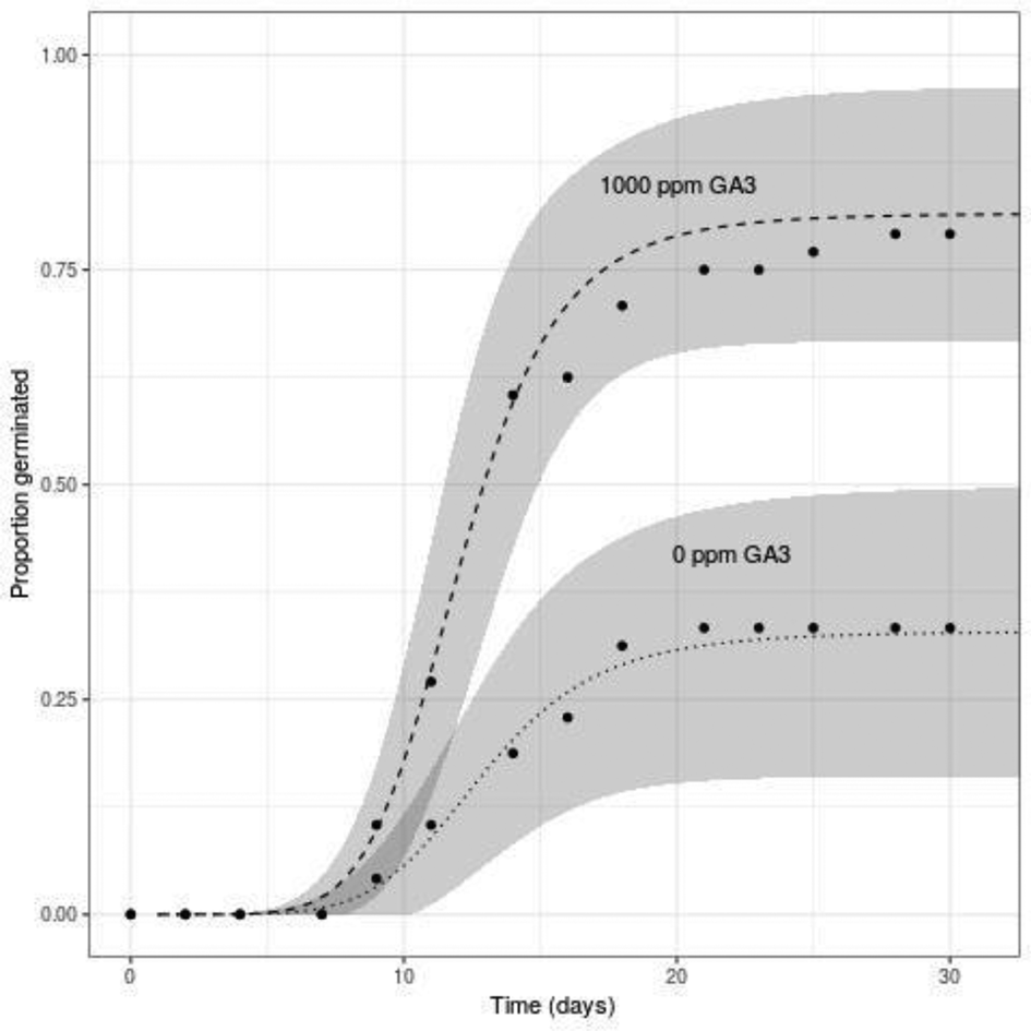
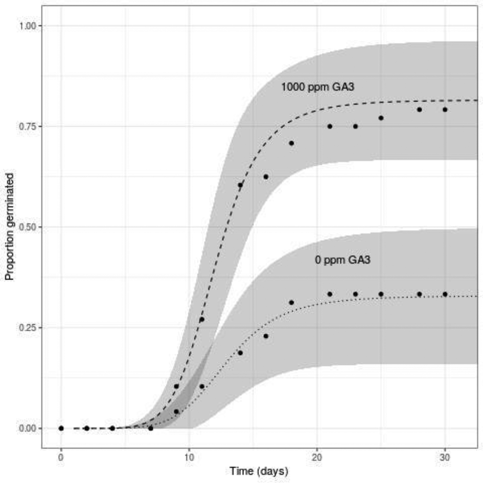
Figure 1 shows the fitted germination curves for 0 (dotted line) and 1000 (dashed line) ppm GA3 with corresponding (marginal) 95% confidence bands. The different maximal rates of germination (upper limits) are reflected in the non-overlapping confidence bands observed from day 13 and onward. It is also noteworthy that the fitted germination curve for the high concentration of 1000 ppm GA3 does not fit all data points equally well: there is an almost perfect fit up to almost 15 d (the time period where most seeds germinated), but then the fitted curve overshoots the observed data. The maximal rate of germination seems to be reached more rapidly than anticipated by the three-parameter log-logistic model. This is surprising as this feature was not apparent when looking at the individual model fits in Step 1 where the log-logistic model seemed appropriate (shown in the detailed results deposited online).
The effect of two concentrations of gibberellic acid on germination of E. sparganophyllum seeds: Two-fitted germination curves with corresponding 95% confidence bands based on the improved two-step analysis where replicate-specific three-parameter log-logistic models (equation 1) were fitted and combined using meta-analysis.
Example 2
For a total of 122 pots, the three-parameter log-logistic model could be fitted in Step 1. The automated model fitting failed for another six pots: five pots at a depth of 6 cm and one pot at a depth of 0 cm. For the pots at depth 6 cm, inspection of the data revealed that failure was due to no observed germination, implying that these pots provided no information on any parameters as the corresponding fitted seed germination curves were flat, horizontal lines coinciding with the time axis. For the pot at depth 0 cm, it was possible to manually fit an event-time model assuming a two-parameter log-logistic model (where the upper limit is fixed at 1) as all seeds germinated in this pot. Consequently, the data used in Step 2 were slightly unbalanced with a sample size of 368 ( = 122 ⋅ 3 + 1 ⋅ 2).
The linear mixed model in Step 2 was successfully fitted, but it took a few minutes due to the estimation of several correlations. Model checking by means of residual and QQ plots showed excellent agreement with the model assumptions (plots shown in the Supplementary material). The estimated standard deviations for the between-replication variation were small [0.88 (unitless), 0.03 (on the probability scale) and 6.72 (in hours) for the parameters b, d and t 50, respectively]. However, these estimates were based on only two replications, which naturally provided very little information. The estimated standard deviations for the between-pot variation were mostly somewhat larger [0.72 (unitless), 0.07 (on the probability scale) and 16.82 (in hours) for the parameters b, d and t 50, respectively] and, as they reflected variation between 122 pots, these standard deviations were much more precisely estimated.
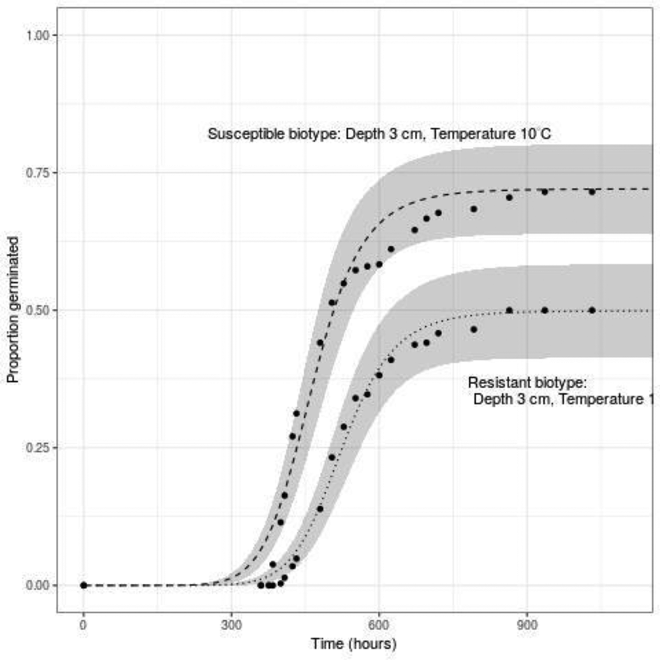
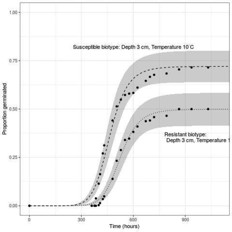
For a depth of 3 cm and a temperature of 10°C, the resistant biotype compared to the susceptible biotype had an estimated slope that was 0.94 (95% CI: −1.00, 2.87) smaller, an estimated maximal rate of germination that was 0.22 (95% CI: 0.12, 0.33) lower and an estimated t 50 that was 57 (95% CI: 32, 84) hours larger.
Figure 2 shows the corresponding fitted seed germination curves (dotted line for the resistant biotype, dashed line for the susceptible biotype) with the 95% confidence bands, which for almost the entire time axis do not overlap, confirming that two combinations were different in terms of the maximal rate of germination as well as t 50.
The difference in germination between resistant and susceptible biotypes of black grass for a specific depth and temperature: Two-fitted germination curves with corresponding 95% confidence bands based on the improved two-step analysis where pot-specific three-parameter log-logistic models (equation 1) were fitted and combined using meta-analysis.
Discussion
We propose an improved and flexible two-step meta-analytic approach that enables convenient visualization of fitted germination curves. This means that observed cumulated germination data may be shown together with the corresponding fitted germination curves and confidence bands, which are based on statistical analysis that incorporates all sources of variation present in even complex germination experiments.
Moreover, we have provided a much more comprehensive description of the workflow when carrying out the two-step approach in practice as documented in the detailed Supplementary material. In particular, we have shown how to incorporate manual model fits in case automated model fitting fails and we have shown how to check modelling assumptions both in Step 1 and Step 2.
One limitation of the proposed approach is that the joint linear mixed models may become difficult to fit for very large experiments as the estimation of the correlation structure can be challenging. The simpler joint model assuming uncorrelated parameter estimates (assuming a diagonal variance–covariance matrix) may be easier to fit in such situations without much loss in efficiency. Another limitation is the fact that the two-step approaches require a model fit for each sub-experiment. For sub-experiments exhibiting small sample sizes and large variability (insufficient data), it might be difficult to fit a model and there is no option of borrowing of strength across sub-experiments (such that information from other sub-experiments can help obtained a reasonable fit), in contrast to a one-step model such as mixed model if it were available.