1 Introduction
Determining transport of material particles or the advection of larger objects in turbulence is one of the most enduring problems of hydrodynamics with a broad range of applications (Monin & Yaglom Reference Monin and A. M.1975). For instance, particles of very different nature (seeds, pollutants, water droplets) can be carried by turbulence in the atmosphere or transported at the surface of the oceans. Turbulent transport plays an important role in the long-distance dispersal of seeds (Nathan et al. Reference Nathan, Katul, Horn, Thomas, Oren, Avissar, Pacala and Levin2002), in the development of pollution control strategies (Toschi & Bodenschatz Reference Toschi and Bodenschatz2009) or in rain prediction (Falkovich, Fouxon & Stepanov Reference Falkovich, Fouxon and Stepanov2002). In the case of larger objects, a better understanding of turbulent advection is crucial for the development of advanced sea search-and-rescue algorithms (Breivik et al. Reference Breivik, Allen, Maisondieu and Olagnon2013).
The dynamics of a particle advected in any flow depends on how its density and its size compare with the fluid density and a flow characteristic length scale (Guyon et al. Reference Guyon, Hulin, Petit and Mitescu2001). In laminar flows, this comparison is straightforward since such flows usually can be described by a single length scale. In contrast, turbulence is described as a hierarchy of eddies due to the presence of a broad range of scales. It is natural to ask which of these scales affect the most the dynamics of finite-size particles (Monin & Yaglom Reference Monin and A. M.1975; Kraichnan & Montgomery Reference Kraichnan and Montgomery1980). This challenging question makes the prediction of turbulent transport a remarkably difficult problem.
A particle is expected to faithfully follow turbulent fluid motion when it is neutrally buoyant and its size is smaller than the smallest turbulent eddy (Toschi & Bodenschatz Reference Toschi and Bodenschatz2009). Such a particle is called a Lagrangian tracer or more commonly a fluid tracer. The behaviour of fluid tracers in three-dimensional (3D) and two-dimensional (2D) turbulence has been the subject of intense research during the last 20 years, and significant advances have been made in the understanding of the Lagrangian properties of turbulence (Elhmaidi, Provenzale & Babiano Reference Elhmaidi, Provenzale and Babiano1993; Mordant et al. Reference Mordant, Metz, Michel and Pinton2001; Boffetta & Sokolov Reference Boffetta and Sokolov2002; Bourgoin et al. Reference Bourgoin, Ouellette, Xu, Berg and Bodenschatz2006; Toschi & Bodenschatz Reference Toschi and Bodenschatz2009; Xia et al. Reference Xia, Francois, Punzmann and Shats2013, Reference Xia, Francois, Punzmann and Shats2014; Xu et al. Reference Xu, Pumir, Falkovich, Bodenschatz, Shats, Xia, Francois and Boffetta2014; Francois et al. Reference Francois, Xia, Punzmann, Faber and Shats2015b ). In contrast, when the advected particle has a density that is different from that of the fluid and/or is of larger size, it can no longer be considered as a tracer and it is commonly called an inertial particle. The dynamics of such particles will deviate from that of the surrounding fluid (Gatignol Reference Gatignol1983; Maxey & Riley Reference Maxey and Riley1983; Qureshi et al. Reference Qureshi, Bourgoin, Baudet, Cartellier and Gagne2007).
The description of the transport of inertial particles in turbulent flows remains an open question which requires insights from experimental studies (Toschi & Bodenschatz Reference Toschi and Bodenschatz2009). For instance, important experiments in 3D turbulence have clarified how inertia affects the acceleration statistics of an advected particle or how it can lead to an apparent clustering of particles (Qureshi et al. Reference Qureshi, Bourgoin, Baudet, Cartellier and Gagne2007; Xu & Bodenschatz Reference Xu and Bodenschatz2008; Toschi & Bodenschatz Reference Toschi and Bodenschatz2009).
Here we focus on the transport of inertial particles in 2D turbulence. The domain of application of 2D turbulence has recently been broadened with the realisation that many 3D flows actually show properties consistent with 2D turbulence (see Falkovich et al. (Reference Falkovich, Boffetta, Shats and Lanotte2017) and Xia & Francois (Reference Xia and Francois2017) for recent reviews). Two-dimensional turbulence differs from 3D turbulence in many aspects. One important difference is that energy injected at an intermediate forcing scale
 $L_{f}$
is transferred to larger scales in a process known as the inverse energy cascade (Kraichnan Reference Kraichnan1967). To date, experimental effort on inertial particles in 2D turbulence has primarily focused on particles with sizes much smaller than
 $L_{f}$
(Ouellette, O’Malley & Gollub Reference Ouellette, O’Malley and Gollub2008). In this work we are interested in dispersion of neutrally floating discs placed in the wave-driven 2D turbulence (von Kameke et al.
Reference von Kameke, Huhn, Fernández-García, Muñuzuri and Pérez-Muñuzuri2011; Francois et al.
Reference Francois, Xia, Punzmann and Shats2013). We investigate the dynamics of these objects in a broad range of sizes
 $r_{p}$
relative to the turbulent forcing scale
 $L_{f}$
. All these objects disperse diffusively at long times and their diffusion coefficient
 $D$
is measured as a function of their radius
 $r_{p}$
, of the flow kinetic energy
 $U^{2}$
and for different forcing scale
 $L_{f}$
. We show that the dependence of
 $D$
on these parameters undergoes a sharp change for values of the object size close to the forcing scale
 $r_{p}\approx L_{f}$
. When
 $r_{p}/L_{f}$
is large, objects are dispersed slowly by the turbulence and the diffusion coefficient
 $D$
scales as
 $D\sim U^{2}/r_{p}$
. Small objects,
 $r_{p}<L_{f}$
, are dispersed much faster and
 $D$
scales as
 $D\sim U/r_{p}^{0.35}$
. We show that the transition is related to the underlying fabric of wave-driven turbulence which consists of anisotropic river-like structures whose width is comparable to
 $L_{f}$
. In the context of controlling the motion of floating objects by using surface waves (Chen et al.
Reference Chen, Luo, Guven, Tasoglu, Ganesan, Weng and Demirci2014; Punzmann et al.
Reference Punzmann, Francois, Xia and Shats2014; Francois et al.
Reference Francois, Xia, Punzmann, Fontana and Shats2017), these results offer methods to externally tune the diffusion coefficient of a floating object at a liquid surface perturbed by Faraday waves.
2 Experiments
2.1 Experimental protocol and data analysis
In these experiments, turbulent flows are produced on a liquid surface perturbed by Faraday waves (Faraday Reference Faraday1831). These parametrically excited waves are generated in a 290 mm diameter circular container filled with water up to its brim (the contact line is pinned to the wall edge with no meniscus). The container is vertically vibrated by a computer-controlled electrodynamic shaker. The forcing is monochromatic with a frequency set in the range
 $f_{s}=15{-}60~\text{Hz}$
. The amplitude of the vertical acceleration
 $a$
of the container is measured by an accelerometer that provides feedback to the system motion controller. Above a critical vertical acceleration, parametrically excited waves, or Faraday waves, appear at the liquid–gas interface. When the Faraday waves are steep, the wave motion is disordered (Xia, Shats & Punzmann Reference Xia, Shats and Punzmann2010; Francois et al.
Reference Francois, Xia, Punzmann and Shats2015a
). We study the flows generated by these waves (Hansen et al.
Reference Hansen, Schröder, Alstrøm, Andersen and Levinsen1997; von Kameke et al.
Reference von Kameke, Huhn, Fernández-García, Muñuzuri and Pérez-Muñuzuri2011; Francois et al.
Reference Francois, Xia, Punzmann and Shats2013, Reference Francois, Xia, Punzmann and Shats2015a
) in the range of vertical accelerations
 $a$
that correspond to the supercriticality factor of
 $0.5<\unicode[STIX]{x1D716}<3$
, where
 $\unicode[STIX]{x1D716}=(a-a_{th})/a_{th}$
and
 $a_{th}$
is the instability threshold of the Faraday waves. This method of turbulence generation relies on the ability of waves to generate vorticity at the fluid surface (Punzmann et al.
Reference Punzmann, Francois, Xia and Shats2014; Francois et al.
Reference Francois, Xia, Punzmann, Ramsden and Shats2014, Reference Francois, Xia, Punzmann, Fontana and Shats2017).
In this study, we are interested in the dispersion properties of large floating discs placed in the wave-driven flows. The liquid surface is seeded with microscopic floating tracers to visualise horizontal fluid motion. We use surfactant to reduce the particle propensity to aggregate. A high-resolution video camera (Andor Zyla) is used to record the motion of fluid tracers and large floating discs. The large floating discs are printed on a high-resolution 3D printer (Ultimaker 2+). The floaters studied here have a radius
 $r_{p}$
in the range of
 $r_{p}=0.5{-}40~\text{mm}$
and are made of a thermoplastic polymer (acrylonitrile butadiene styrene (ABS)). The density of the polymer matches that of water and the disc thickness is 0.5 mm. After printing, the floaters are carefully rinsed using water with surfactant and are kept in a water beaker for 24 hours to ensure they release any residual substances that could potentially pollute the water surface. In steep waves the floating disc might get gradually covered with a thin film of water; to ensure the top of the disc remains dry throughout the experiments, their top surfaces were coated with Teflon.
Quantitative data analysis of the flow and the dynamics of the large discs is performed by using particle image velocimetry (PIV) and particle tracking velocimetry (PTV) algorithms (Francois et al.
Reference Francois, Xia, Punzmann, Ramsden and Shats2014). The flow characterisation (based on both PIV and PTV) was performed with tracers with a diameter of either
 $50~\unicode[STIX]{x03BC}\text{m}$
or
 $150~\unicode[STIX]{x03BC}\text{m}$
. No effect of the tracer size was detected on these measurements: the two types of tracers provide very similar Eulerian and Lagrangian descriptions of the flow. For the PTV measurements, a typical sample of trajectories consists of 2000 trajectories. The PIV technique is used to obtain velocity fields of the horizontal fluid motion. During experiments, the motion of the fluid tracers is recorded at a frame rate of 120 frames per second to characterise flows of root-mean-square (r.m.s.) velocity
 $0.01<U<0.05~\text{m}~\text{s}^{-1}$
. For most of the data based on the PIV technique presented in the main text, the field of view used for the analysis is
 $80~\text{mm}\times 80~\text{mm}$
. The spatial resolution is
 $100~\unicode[STIX]{x03BC}\text{m}$
per pixel. The velocity fields are computed on a
 $100\times 100$
spatial grid (grid mesh size is
 ${\approx}0.8~\text{mm}$
), with a
 $1.6~\text{mm}\times 1.6~\text{mm}$
interrogation window size (the interrogation windows overlap). The measurement resolution of the instantaneous displacement is subpixel.
In the analysis presented in § 3.4, fluid particle trajectories are reconstructed by integrating the high-resolution velocity field measured using the PIV technique (Sokolov & Reigada Reference Sokolov and Reigada1999; Rivera & Ecke Reference Rivera and Ecke2016). Particle trajectories are obtained by integrating the equations of motion of particles starting from a given initial point
 $x(t_{0})$
, as
 $\text{d}\boldsymbol{x}(t)/\text{d}t=\boldsymbol{u}(\boldsymbol{x},t)$
. Here
 $\boldsymbol{x}(t)$
is a particle 2D coordinate and
 $\boldsymbol{u}(\boldsymbol{x},t)$
is the velocity field measured using PIV. The particles advected by the flow are tracked using the fourth-order Runge–Kutta method. In this study, the method is used to reconstruct the trajectories of virtual particles initially placed on a grid with a mesh size of
 ${\approx}0.15~\text{mm}$
. On a technical note, this method allows one to overcome the common experimental limitations of PTV encountered when a high density of fluid tracers is used, and therefore allows one to probe with accuracy the fine Lagrangian properties of turbulence such as higher-order statistical moments. As an additional test, we have also checked that the transport properties (single-particle dispersion and topological multi-particle descriptor) computed from the integrated trajectories are identical to those obtained using PTV and reported in Xia et al. (Reference Xia, Francois, Punzmann and Shats2013) and Francois et al. (Reference Francois, Xia, Punzmann, Faber and Shats2015b
).
2.2 Faraday wave-driven two-dimensional turbulence
Although energy is injected into vertical motion of a liquid, part of this energy is converted into turbulent horizontal fluid motion via the generation and interaction of surface vortices (Francois et al.
Reference Francois, Xia, Punzmann, Ramsden and Shats2014). These wave-driven flows are random, have no mean velocity and their dynamics is slow compared to the period of vertical oscillations in the wave. The kinetic energy of the horizontal flow
 $E_{f}$
is proportional to the square of the horizontal velocity fluctuations,
 $E_{f}\sim U^{2}$
(
 $U$
is the r.m.s. value of the fluctuations). The flow forcing scale is
 $L_{f}=\unicode[STIX]{x1D706}/2$
, where
 $\unicode[STIX]{x1D706}$
is the Faraday wavelength. Since the wavelength
 $\unicode[STIX]{x1D706}$
is a function of the forcing frequency
 $f_{s}$
, the flow forcing scale
 $L_{f}$
can be easily tuned by changing
 $f_{s}$
(Hansen et al.
Reference Hansen, Schröder, Alstrøm, Andersen and Levinsen1997; Francois et al.
Reference Francois, Xia, Punzmann and Shats2013). In these experiments,
 $L_{f}$
is in the range
 $4{-}20~\text{mm}$
. The forcing scale Reynolds number,
 $Re=UL_{f}/\unicode[STIX]{x1D708}$
(where
 $\unicode[STIX]{x1D708}$
is the kinematic viscosity of water), is in the range of 45–180.
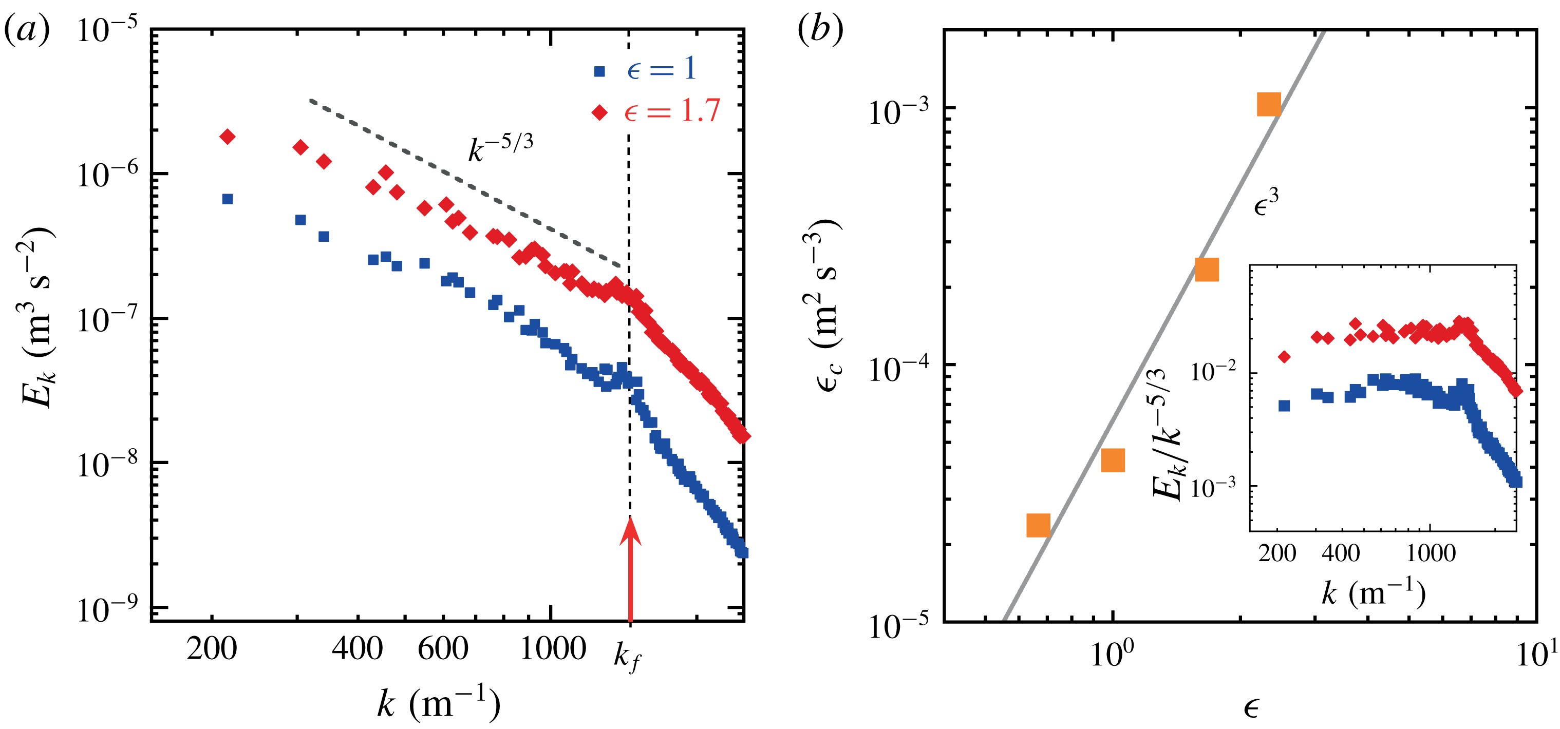
(a) Wavenumber spectra of kinetic energy
 $E_{k}(k)$
of the horizontal flow for increasing supercriticality parameter
 $\unicode[STIX]{x1D716}=(a-a_{th})/a_{th}$
. (b) Energy injection rate
 $\unicode[STIX]{x1D716}_{c}$
versus supercriticality parameter
 $\unicode[STIX]{x1D716}$
. Here
 $\unicode[STIX]{x1D716}_{c}=(E(k)/C)^{3/2}k^{5/2}$
is measured from the energy spectra shown in panel (a);
 $C=6$
is the Kolmogorov constant for 2D turbulence. Inset: compensated wavenumber spectra
 $E_{k}(k)/k^{-5/3}$
of the kinetic energy.

The r.m.s. fluid velocity
 $U$
depends on the kinetic energy accumulated over a broad range of scales, as demonstrated by computing the wavenumber spectrum of the kinetic energy of the horizontal flow (figure 1
a). Two scaling laws can be identified in these spectra: a
 $k^{-5/3}$
scaling for wavenumbers smaller than the forcing wavenumber
 $k_{f}\approx 2\unicode[STIX]{x03C0}/L_{f}$
(see also inset of figure 1
b), while for larger wavenumbers, the scaling becomes much steeper and is approximately equal to
 $k^{-3}$
. The
 $k^{-5/3}$
scaling is consistent with Kraichnan’s prediction of a 2D inverse energy cascade. It indicates that the wave-driven flows support spectral energy transfer from the forcing scale to large scales (von Kameke et al.
Reference von Kameke, Huhn, Fernández-García, Muñuzuri and Pérez-Muñuzuri2011; Francois et al.
Reference Francois, Xia, Punzmann and Shats2013, Reference Francois, Xia, Punzmann, Ramsden and Shats2014; Xia & Francois Reference Xia and Francois2017). The
 $k^{-3}$
scaling is consistent with the (direct) enstrophy cascade range. The kinetic energy of the flow
 $U^{2}$
depends almost entirely on the energy accumulated over the
 $k^{-5/3}$
range. The energy injection rate
 $\unicode[STIX]{x1D716}_{c}$
in the upscale cascade can be computed as
 $\unicode[STIX]{x1D716}_{c}=(E(k)/C)^{3/2}k^{5/2}$
, where
 $C=6$
is the Kolmogorov constant. Figure 1(b) shows
 $\unicode[STIX]{x1D716}_{c}$
as a function of the wave supercriticality factor
 $\unicode[STIX]{x1D716}$
. It is found that
 $\unicode[STIX]{x1D716}_{c}$
increases strongly with
 $\unicode[STIX]{x1D716}$
and its behaviour can be approximated by
 $\unicode[STIX]{x1D716}_{c}\sim \unicode[STIX]{x1D716}^{3}$
. The Taylor-microscale Reynolds number
 $Re_{\unicode[STIX]{x1D6EC}}=U\unicode[STIX]{x1D6EC}/\unicode[STIX]{x1D708}$
can be estimated using the Taylor microscale
 $\unicode[STIX]{x1D6EC}=\sqrt{U/\unicode[STIX]{x1D6FA}}$
, where
 $\unicode[STIX]{x1D6FA}$
is the enstrophy of the flow. Quantitatively,
 $\unicode[STIX]{x1D6EC}\approx 2~\text{mm}$
in experiments performed at
 $f_{s}=60~\text{Hz}$
and
 $Re_{\unicode[STIX]{x1D6EC}}$
is between 25 and 100.
Faraday flows are indisputably 3D on the time scale of a wave period, yet we have just discussed the fact that on larger time scales the motion of floating tracers reproduces properties of 2D turbulence. Recently, the question of the dimensionality of Faraday flows was addressed by investigating the compressibility of the horizontal velocity field, in particular its time dependence (Xia & Francois Reference Xia and Francois2017). This approach was based on the computation of a compressibility parameter that allows one to measure 3D effects quantitatively (Cressman et al. Reference Cressman, Davoudi, Goldburg and Schumacher2004). When this parameter is averaged over a few wave periods, it takes a value similar to that measured in double-layer electromagnetically forced turbulence, which is widely accepted as a good laboratory model of 2D flows. This confirms the quasi-2D and quasi-incompressible nature of the slow (compared to the wave frequency) horizontal motion produced by the Faraday waves. Moreover, we also note that the floating tracers stay homogeneously distributed over the water surface perturbed by Faraday waves. This is strong evidence that the 2D flow generated by the waves can be considered incompressible since a compressible surface flow would induce substantial floater clustering (Cressman et al. Reference Cressman, Davoudi, Goldburg and Schumacher2004).
2.3 Measuring turbulent dispersion in model experiments
The theory of diffusion by turbulent motion dates back to Taylor (Reference Taylor1921). Taylor introduced a conceptual framework in which the single-particle dispersion in turbulence is governed by the stochastic equation. He discussed the case of a fluid particle evolving in an unbounded turbulent flow and tackled the behaviour of the mean-squared displacement (MSD)
 $\langle \unicode[STIX]{x1D6FF}r^{2}\rangle =\langle |\boldsymbol{r}(t)-\boldsymbol{r}(0)|^{2}\rangle$
, where
 $\boldsymbol{r}(t)$
is the position of the particle at time
 $t$
and
 $\langle ~\rangle$
denotes statistical averaging. When the fluid particle dynamics can be described as a process having a finite velocity variance
 $U^{2}$
and a finite memory characterised by a time scale
 $T_{f}$
, an important result is that a transition exists in the MSD between a so-called ballistic regime and a diffusive behaviour characterised by a diffusion coefficient
 $D$
.
This theory gives
 $$\begin{eqnarray}\displaystyle & \displaystyle \langle \unicode[STIX]{x1D6FF}r^{2}\rangle \approx U^{2}t^{2},\quad t\ll T_{f}, & \displaystyle\end{eqnarray}$$
 $$\begin{eqnarray}\displaystyle & \displaystyle \langle \unicode[STIX]{x1D6FF}r^{2}\rangle \approx Dt,\quad t\gg T_{f}. & \displaystyle\end{eqnarray}$$
Under the aforementioned conditions, there is a direct kinematic relation between the MSD and the Lagrangian velocity autocorrelation function. Indeed
 $T_{f}=\int _{0}^{\infty }\unicode[STIX]{x1D70C}(\unicode[STIX]{x1D70F})\,\text{d}t$
is the Lagrangian integral time, which can be obtained from integrating
 $$\begin{eqnarray}\unicode[STIX]{x1D70C}(\unicode[STIX]{x1D70F})=\langle \boldsymbol{u}(t_{0}+\unicode[STIX]{x1D70F})\boldsymbol{\cdot }\boldsymbol{u}(t_{0})\rangle /U^{2},\end{eqnarray}$$
where
 $\boldsymbol{u}$
is the velocity vector of the fluid particle. Moreover, the diffusion coefficient is given by
 $D=U^{2}T_{f}$
.
This seminal contribution offers tools for studying turbulent dispersion in model experiments. However the variables of interest (i.e. MSD and
 $T_{f}$
) have been defined for unbounded domains and it is therefore interesting to discuss how such quantities are measured in an experiment which is by nature bounded in space and time.
In this study, we are interested in the dispersion of large floating discs placed in wave-driven turbulence. The typical time of a measurement is
 $T_{m}\approx 20~\text{s}$
and a disc trajectory is tracked in a 20 cm diameter circular window (the container diameter is 29 cm). Under these conditions, we will show that the motion of large floating discs becomes diffusive over a range of temporal and spatial scales. Moreover, we note that the transition from a ballistic to a diffusive regime has already been studied for fluid tracer particles in similar experimental conditions (Xia et al.
Reference Xia, Francois, Punzmann and Shats2013).
In the rest of this study, measurements of the diffusion coefficient
 $D$
, of the disc velocity variance
 $V_{p}^{2}$
and of the autocorrelation function are therefore performed by adapting Taylor’s original formulation to the finite experimental conditions. We will compare two time scales that can be independently measured. From the diffusion coefficient we define
 $T_{disc}=D/V_{p}^{2}$
, which characterises the transition from ballistic to diffusive regime in the MSD. We also measure independently the integral time scale
 $T_{p}$
as
 $T_{p}=\int _{0}^{T_{m}}\unicode[STIX]{x1D70C}(\unicode[STIX]{x1D70F})\,\text{d}t$
.
3 Results
3.1 Turbulent dispersion of finite-size discs
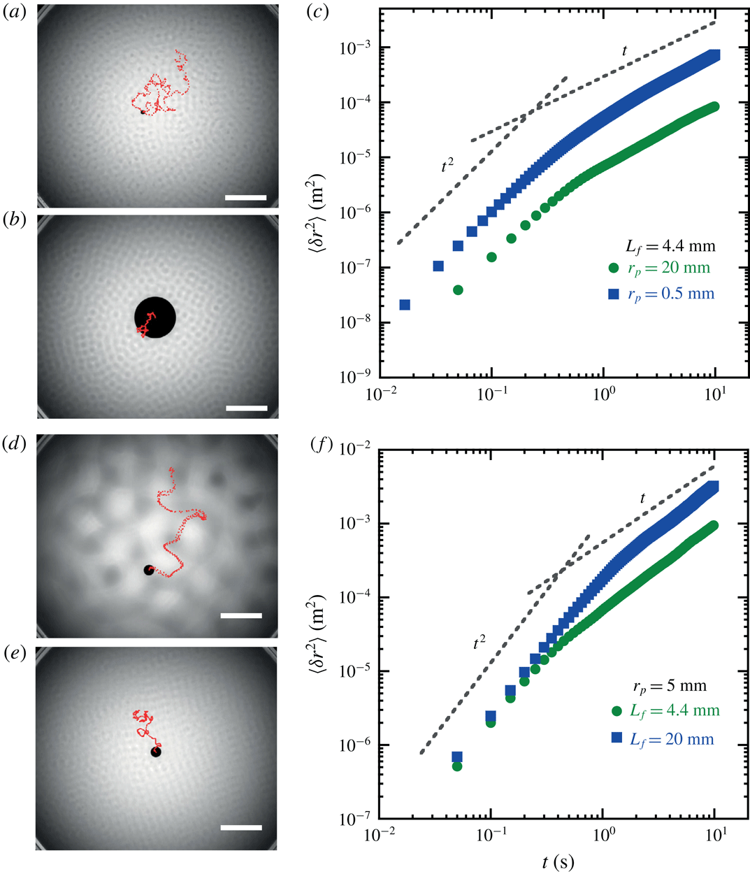
Figure 2(a,b,d,e) shows trajectories of floating discs placed in the wave-driven turbulent flows for three different sizes
 $r_{p}$
. Regardless of their size, the motion of the floaters is erratic. A typical experimental run consists in recording 2000 independent trajectories of a disc of radius
 $r_{p}$
for a given flow energy
 $U^{2}$
and a fixed value of the forcing scale
 $L_{f}$
. We use these statistical samples to characterise the single-particle dispersion of the floating discs. Our main focus is the behaviour of the MSD
 $\langle \unicode[STIX]{x1D6FF}r^{2}(t)\rangle$
as a function of the three parameters
 $U^{2}$
,
 $L_{f}$
and
 $r_{p}$
.
(a,b) Trajectories (red dots) of two floating discs in wave-driven turbulent flows having the same turbulence intensity and the same forcing frequency
 $f_{s}=60~\text{Hz}$
. Two floating discs having diameters
 $d_{p}$
of (a) 4 mm and (b) 40 mm, respectively, are advected with the turbulent flow. The disc centres are tracked for 15 s (scale bars in the bottom right corners are 40 mm). (c) Mean-squared displacement of the disc centres versus time for two particles with diameters 40 mm and 1 mm, respectively. Grey dashed lines highlight the transition from a ballistic to a diffusive regime. Experimental parameters:
 $f_{s}=60~\text{Hz}$
, the flow forcing scale and the turbulent kinetic energy are fixed at
 $L_{f}\approx 4.4~\text{mm}$
and
 $U^{2}=5.5\times 10^{-4}~\text{m}^{2}~\text{s}^{-2}$
. Data are averaged over 2000 independent trajectories. (d,e) Trajectories (red dots) of a floating disc of radius
 $r_{p}=5~\text{mm}$
in turbulent flows forced at two different frequencies: (d)
 $f_{s}=15~\text{Hz}$
,
 $L_{f}\approx 20~\text{mm}$
and (e)
 $f_{s}=60~\text{Hz}$
,
 $L_{f}\approx 4.4~\text{mm}$
. Turbulent kinetic energy in both (d) and (e) is fixed at
 $U^{2}=1.1\times 10^{-3}~\text{m}^{2}~\text{s}^{-2}$
. The disc centres are tracked for 15 s; the scale bar is 40 mm. (f) Mean-squared displacement versus time for the 5 mm radius disc measured at two forcing scales:
 $L_{f}=4.4~\text{mm}$
(circles) and
 $L_{f}=20~\text{mm}$
(squares). Data are averaged over 2000 independent trajectories.

Qualitatively, the motion of all discs shows the same statistical features (figure 2
c,f), namely: a ballistic regime at short times (
 $\langle \unicode[STIX]{x1D6FF}r^{2}\rangle \sim V_{p}^{2}t^{2}$
, at
 $t\ll T_{disc}$
), and a diffusive behaviour at longer times (
 $\langle \unicode[STIX]{x1D6FF}r^{2}\rangle =2Dt$
, at
 $t\gg T_{disc}$
). Here
 $V_{p}^{2}$
is the velocity variance measured on the statistical ensemble of trajectories. As mentioned in the previous section,
 $T_{disc}$
is defined as
 $T_{disc}=D/V_{p}^{2}$
; it characterises the transition from ballistic to diffusive regime in the MSD.
Quantitatively, figure 2(c,f) reveals several interesting features of the dispersive behaviour of the discs. Figure 2(c) shows the MSD of two discs with different sizes when both the forcing scale and the turbulent energy are fixed at
 $L_{f}\approx 4.4~\text{mm}$
and
 $U^{2}=5.5\times 10^{-4}~\text{m}^{2}~\text{s}^{-2}$
, respectively. The behaviour in the ballistic regime clearly shows that the velocity variance
 $V_{p}^{2}$
of the small disc (
 $r_{p}=0.11L_{f}$
) is an order of magnitude larger than that of the large disc (
 $r_{p}=4.5L_{f}$
), while the characteristic times
 $T_{disc}$
are roughly the same for both objects. Since
 $D=V_{p}^{2}T_{disc}$
, the change in
 $V_{p}^{2}$
has a direct consequence on the diffusion: small discs (
 $r_{p}=0.11L_{f}$
) diffuse much faster than larger ones (
 $r_{p}=4.5L_{f}$
).
In contrast, a different parameter is varied in figure 2(f). It shows the MSD of a 10 mm diameter disc placed in turbulent flows with identical turbulent energy (
 $U^{2}=1.1\times 10^{-3}~\text{m}^{2}~\text{s}^{-2}$
) but at two different forcing scales
 $L_{f}$
. Importantly, the forcing scale is chosen such that in one case
 $r_{p}<L_{f}$
while in the other
 $r_{p}>L_{f}$
. The ballistic regime reveals that the velocity variance
 $V_{p}^{2}$
is almost unchanged when
 $L_{f}$
is modified, while
 $T_{disc}$
has clearly changed. Quantitatively
 $T_{disc}$
increases by a factor of 3 when
 $L_{f}$
increases by a factor of 4. Consequently, the disc with small
 $r_{p}/L_{f}$
ratio diffuses faster due to its larger
 $T_{disc}$
.
Figure 2(f) suggests the existence of a threshold value
 $r_{p}/L_{f}=1$
separating two diffusive regimes. To investigate this effect further, we have performed experiments with discs of different sizes placed in turbulent flows with identical turbulent energy and forcing scale (
 $U^{2}=5.5\times 10^{-4}~\text{m}^{2}~\text{s}^{-2}$
,
 $L_{f}=4.4~\text{mm}$
). The measurements of the diffusion coefficient
 $D$
as a function of the disc radius
 $r_{p}$
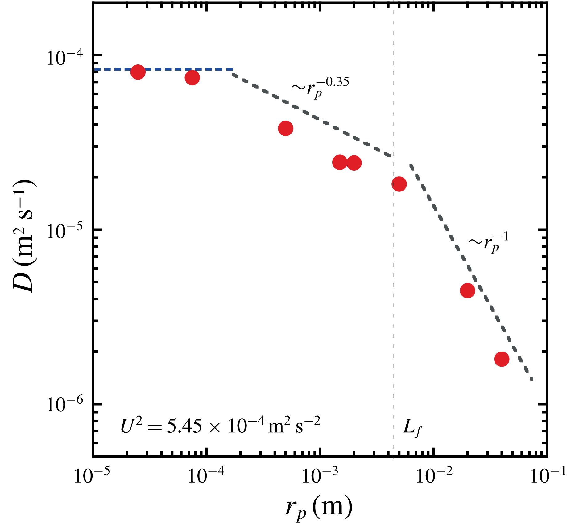
are shown in figure 3. The diffusion coefficient decreases with the radius
 $r_{p}$
. Most importantly, it turns out that the threshold value
 $r_{p}/L_{f}=1$
shows up clearly in this experiment. At high value of the ratio
 $r_{p}/L_{f}>1$
, the coefficient
 $D$
is inversely proportional to the radius
 $r_{p}$
. In the low-value domain
 $r_{p}/L_{f}<1$
, the dependence is weaker and can be fitted by the scaling law
 $D\sim 1/r_{p}^{0.35}$
. The coefficient
 $D$
eventually saturates to a constant value for fluid tracers.
Figure 2(c,f) and figure 3 reflect different information about the disc–turbulence coupling. They show that the dispersive properties of finite-size discs in turbulence depend on the disc radius
 $r_{p}$
but also on the flow forcing scale
 $L_{f}$
and on how those two parameters affect the disc kinetic energy and its memory. Our main interest in this paper is the diffusive regime with a diffusion coefficient given by
 $D=V_{p}^{2}T_{disc}$
. To better understand the previous observations, we will study the behaviour of the velocity variance
 $V_{p}^{2}$
and of the characteristic time
 $T_{disc}$
separately.
Diffusion coefficient
 $D$
as a function of the disc radius
 $r_{p}$
. The flow energy
 $U^{2}$
and the forcing scale
 $L_{f}$
are fixed. The vertical dashed line indicates the forcing scale
 $L_{f}$
. The coefficient measured for fluid tracers (
 $r=50~\unicode[STIX]{x03BC}\text{m}$
) is indicated. The horizontal blue line indicates the diffusion coefficient measured from the motion of virtual tracers obtained by integration of the PIV measurements. (Experimental parameters:
 $f_{s}=60~\text{Hz}$
,
 $L_{f}\approx 4.4~\text{mm}$
,
 $U^{2}=5.45\times 10^{-4}~\text{m}^{2}~\text{s}^{-2}$
.)

3.2 Kinetic energy of finite-size discs
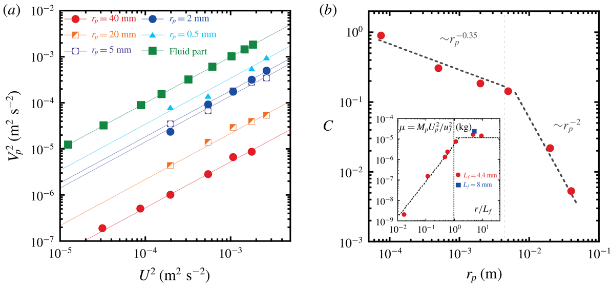
(a) Velocity variance of floating discs
 $V_{p}^{2}$
of various sizes versus the flow energy
 $U^{2}$
. The forcing scale
 $L_{f}$
is fixed. The dashed lines are linear fits. (b) Ratio
 $C=V_{p}^{2}/U^{2}$
as a function of the disc radius
 $r_{p}$
. The vertical dashed line indicates the forcing scale
 $L_{f}$
. (Experimental parameters:
 $f_{s}=60~\text{Hz}$
,
 $L_{f}\approx 4.4~\text{mm}$
.) Inset: Parameter
 $\unicode[STIX]{x1D707}=M_{p}V_{p}^{2}/U^{2}$
versus the size ratio
 $r_{p}/L_{f}$
.

In this section we study the dependence of the velocity variance
 $V_{p}^{2}$
of the floating discs on the turbulent flow energy
 $U^{2}$
, the forcing scale
 $L_{f}$
and the disc radius
 $r_{p}$
.
Figure 4(a) shows the velocity variance
 $V_{p}^{2}$
as a function of the flow energy
 $U^{2}$
for a broad range of disc sizes and a fixed forcing scale
 $L_{f}\approx 4.4~\text{mm}$
. In agreement with the data shown in figure 2(c), the smaller the size of the disc, the larger
 $V_{p}^{2}$
is. An important feature of all our experiments is that
 $V_{p}^{2}$
can be fitted accurately by
 $V_{p}^{2}=C\times U^{2}$
. The parameter
 $C=V_{p}^{2}/U^{2}$
decreases with
 $r_{p}$
as shown in figure 4(b). This figure clearly shows a transition in the behaviour of
 $C$
occurring at
 $r_{p}/L_{f}=1$
. For large objects (
 $r_{p}/L_{f}>1$
), the parameter
 $C$
is inversely proportional to the square of the radius, i.e.
 $C\approx (L_{f}/r_{p})^{2}$
. For objects with radius smaller than
 $L_{f}$
, the dependence is weaker and can be fitted by the scaling law
 $C\approx (L_{f}/r_{p})^{0.35}$
.
In these strongly out-of-equilibrium flows, the existence of the fit
 $V_{p}^{2}=C\times U^{2}$
is not trivial and it suggests a simple relation between the disc kinetic energy and the flow energy. To test this conjecture, we compute the parameter
 $\unicode[STIX]{x1D707}=M_{p}V_{p}^{2}/U^{2}$
, where
 $M_{p}$
is the mass of the disc. The parameter
 $\unicode[STIX]{x1D707}$
has the dimension of a mass. The behaviour of
 $\unicode[STIX]{x1D707}$
as a function of the disc radius
 $r_{p}$
is shown in the inset of figure 4(b). This inset reveals two regimes. When
 $r_{p}/L_{f}>1$
, the parameter
 $\unicode[STIX]{x1D707}$
is constant and a simple relation can be written between the kinetic energy of the disc and that of the fluid. At lower values of the size parameter
 $r_{p}/L_{f}<1$
, the parameter
 $\unicode[STIX]{x1D707}$
is no longer constant but it increases with
 $r_{p}$
according to
 $\unicode[STIX]{x1D707}\sim r_{p}^{1.65}$
.
The results of this section again highlight a transition in the coupling between finite-size disc and turbulence that occurs at
 $r_{p}/L_{f}=1$
.
3.3 Temporal memory of finite-size discs
Since the transition to a diffusive dynamics signals a loss of memory, in this section we study the temporal properties of the disc motion. First we compute the Lagrangian velocity autocorrelation function,
 $$\begin{eqnarray}\unicode[STIX]{x1D70C}_{p}(\unicode[STIX]{x1D70F})=\langle \boldsymbol{V}_{p}(t_{0}+\unicode[STIX]{x1D70F})\boldsymbol{\cdot }\boldsymbol{V}_{p}(t_{0})\rangle /V_{p}^{2},\end{eqnarray}$$
where
 $\boldsymbol{V}_{p}$
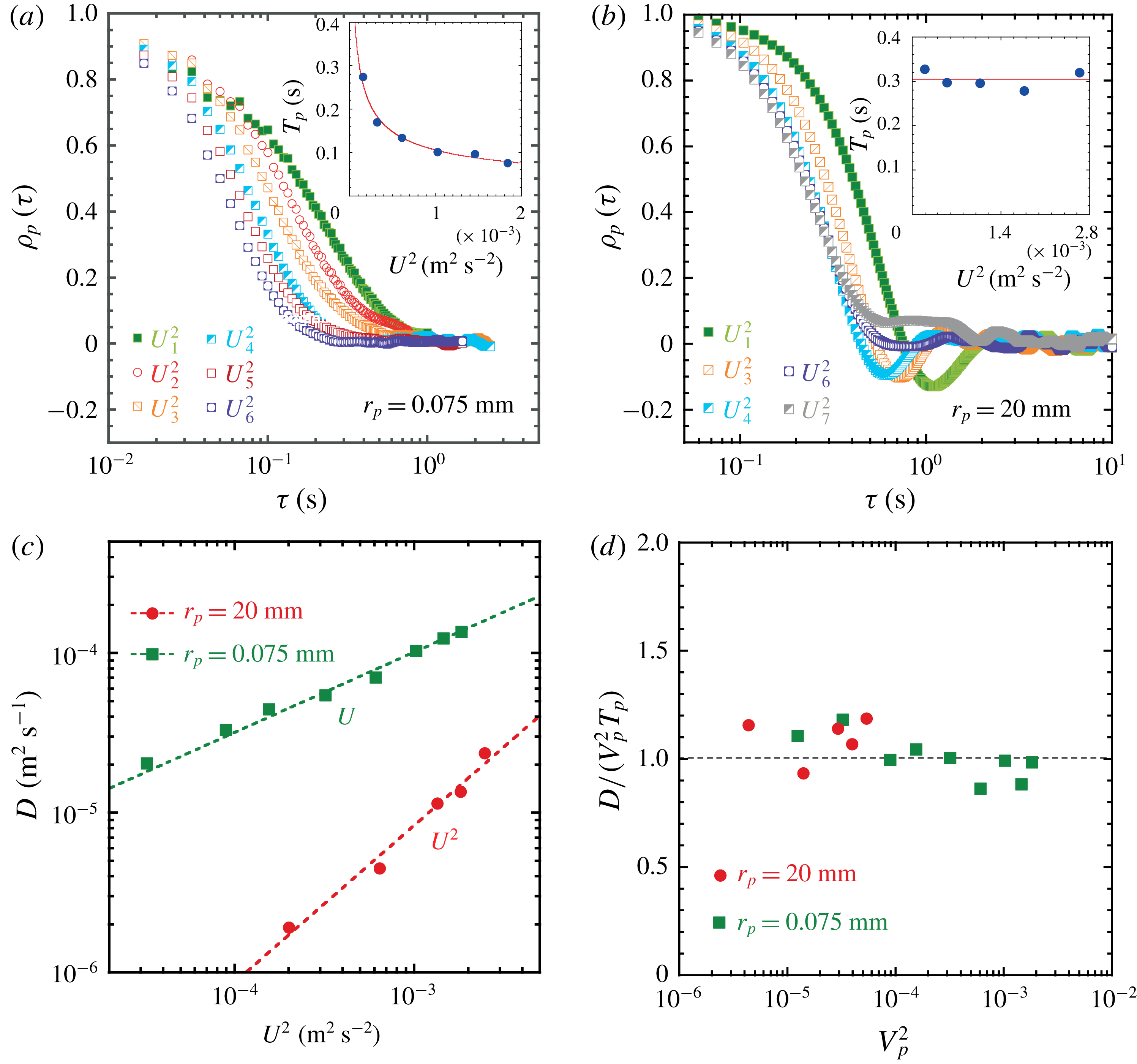
is the velocity vector of the disc. In figure 5(a,b), we show how
 $\unicode[STIX]{x1D70C}_{p}(\unicode[STIX]{x1D70F})$
depends on the turbulent flow energy
 $U^{2}$
and the disc radius
 $r_{p}$
at fixed forcing scale
 $L_{f}=4.4~\text{mm}$
. All these autocorrelation functions are decaying integrable functions of time. Therefore a Lagrangian integral time can be computed as
 $T_{p}=\int _{0}^{T_{m}}\unicode[STIX]{x1D70C}_{p}(\unicode[STIX]{x1D70F})\,\text{d}t$
, where
 $T_{m}$
is the time of the measurement as discussed in § 2.2. In these figures, a clear difference appears between discs larger than
 $L_{f}$
and those smaller than
 $L_{f}$
. For the smaller discs, the autocorrelation function
 $\unicode[STIX]{x1D70C}_{p}(\unicode[STIX]{x1D70F})$
is strongly dependent on the flow kinetic energy
 $U^{2}$
, and
 $\unicode[STIX]{x1D70C}_{p}(\unicode[STIX]{x1D70F})$
decreases faster with the increase in the flow energy. Consequently the integral time
 $T_{p}$
decreases with the increase in
 $U^{2}$
and we find the relation
 $T_{p}\sim 1/U$
(see the inset of figure 5
a). In contrast,
 $\unicode[STIX]{x1D70C}_{p}(\unicode[STIX]{x1D70F})$
is weakly affected by a change in the flow energy in the case of larger discs (
 $r_{p}=4.5L_{f}$
) as shown in figure 5(b). The associated integral time
 $T_{p}$
of these large discs is constant when plotted against the flow energy
 $U^{2}$
(see the inset of figure 5
b). These figures suggest a transition in the memory of the disc from
 $T_{p}\sim 1/U$
for small discs to a time scale
 $T_{p}$
independent of
 $U$
for larger discs.
Temporal autocorrelation functions
 $\unicode[STIX]{x1D70C}_{p}(\text{d}t)=\langle \boldsymbol{V}_{p}(t_{0}+\text{d}t)\boldsymbol{\cdot }\boldsymbol{V}_{p}(t_{0})\rangle /V_{p}^{2}$
computed (a) for particles of radius
 $r_{p}=75~\unicode[STIX]{x03BC}\text{m}$
and (b) for a disc of radius
 $r_{p}=20~\text{mm}$
. These functions are measured for increasing flow energy levels
 $U^{2}$
and at fixed forcing scale
 $L_{f}$
. Insets: Lagrangian integral time
 $T_{p}$
versus
 $U^{2}$
. (Experimental parameters:
 $f_{s}=60~\text{Hz}$
,
 $L_{f}\approx 4.4~\text{mm}$
,
 $U_{i}^{2}=[1.5\times 10^{-4},3.5\times 10^{-4},6.2\times 10^{-4},1\times 10^{-3},1.4\times 10^{-3},1.9\times 10^{-3},2.6\times 10^{-3}]~\text{m}^{2}~\text{s}^{-2}$
.) (c) Diffusion coefficient
 $D$
as a function of the flow energy
 $U^{2}$
for two different particle sizes
 $r_{p}=20~\text{mm}$
and
 $r_{p}=75~\unicode[STIX]{x03BC}\text{m}$
at fixed forcing scale
 $L_{f}$
. (Experimental parameters:
 $f_{s}=60~\text{Hz}$
,
 $L_{f}\approx 4.4~\text{mm}$
.) (d) Diffusion coefficient
 $D$
measured from the MSD normalised by the product of velocity variance
 $V_{p}^{2}$
and the integral time scale
 $T_{p}$
.

Such a transition should have a clear signature in the diffusion coefficient of the disc. In figure 5(c) we test this hypothesis. It shows the diffusion coefficient
 $D$
as a function of the flow energy
 $U^{2}$
for the two disc sizes studied in figure 5(a,b). For the large discs (
 $r_{p}/L_{f}=4.5$
) the diffusion coefficient is proportional to the flow kinetic energy, while for the small discs
 $D$
is proportional to the flow r.m.s. velocity
 $U$
. In other words,
 $D\sim (U^{2})^{\unicode[STIX]{x1D6FD}}$
, where
 $\unicode[STIX]{x1D6FD}=0.5$
for small floaters and
 $\unicode[STIX]{x1D6FD}=1$
for large ones.
(a) Plot of
 $T_{disc}=D/V_{p}^{2}$
as a function of
 $r_{p}$
at fixed flow energy and forcing scale (
 $U^{2}=1\times 10^{-3}~\text{m}^{2}~\text{s}^{-2}$
,
 $L_{f}\approx 4.4~\text{mm}$
). The red dashed line is a linear fit to data in the size range
 $r_{p}>L_{f}$
. (b) Exponent
 $\unicode[STIX]{x1D6FC}$
, derived from
 $T_{disc}\sim (U)^{\unicode[STIX]{x1D6FC}}$
, as a function of the ratio
 $r_{p}/L_{f}$
.

At this point, since our experiments are performed in bounded conditions (see § 2.2), we need to verify that the diffusion coefficient
 $D$
and the integral time
 $T_{p}$
are simply related. Figure 5(d) shows that the ratio of the diffusion coefficient
 $D$
over the product
 $V_{p}^{2}T_{p}$
is close to 1 over the range of flow energy
 $U^{2}$
studied. There is a direct equivalence
 $T_{disc}=D/V_{p}^{2}=T_{p}$
. Therefore
 $T_{disc}$
characterises both the transition from the ballistic to the diffusive regime seen in the MSD and the properties of the autocorrelation function.
In figure 6, we clarify the behaviour of
 $T_{disc}$
as a function of the three parameters
 $r_{p}$
,
 $U^{2}$
and
 $L_{f}$
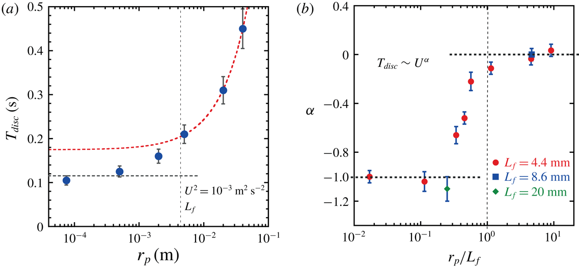
. Figure 6(a) shows the dependence of
 $T_{disc}$
on
 $r_{p}$
when both the flow energy and the forcing scale are fixed. The
 $T_{disc}$
value increases with the disc radius
 $r_{p}$
; more precisely, at large size (
 $r_{p}>L_{f}$
),
 $T_{disc}$
increases linearly with
 $r_{p}$
, while for small discs,
 $T_{disc}$
saturates to a constant value. This constant is given by
 $T_{p}\sim L_{f}/U$
, which is consistent with the behaviour of fluid tracers reported in Xia et al. (Reference Xia, Francois, Punzmann and Shats2013).
In figure 5(c) a transition in the exponent
 $\unicode[STIX]{x1D6FD}$
defined as
 $D\sim (U^{2})^{\unicode[STIX]{x1D6FD}}$
has been identified. It is convenient to characterise this transition from a memory perspective via the relation
 $T_{disc}=D/V_{p}^{2}\sim U^{\unicode[STIX]{x1D6FC}}$
, because it has been shown that
 $V_{p}^{2}=C\times U^{2}$
independently of the disc radius (figure 4
a). Figure 6(b) shows the dependence of the exponent
 $\unicode[STIX]{x1D6FC}$
on the size ratio
 $r_{p}/Lf$
. A transition occurs at
 $r_{p}/L_{f}=1$
; it separates the behaviour of large discs governed by a time scale independent of the flow energy from that of the small discs whose memory is characterised by the relation
 $T_{disc}\sim 1/U$
.
The diffusive nature of a transport phenomenon is an indication of a process with a loss of temporal memory. This memory is characterised by the time scale
 $T_{disc}$
. The transitions observed in the time scale
 $T_{disc}$
in figure 6(a,b) occur at a precise disc size
 $r_{p}=L_{f}$
. In the next sections, we will show that these transitions actually reflect the structure of the wave-driven turbulent flows, in particular the coexistence of random turbulent fluctuations with more coherent flow features.
Statistics of the turbulent flows. (a) Autocorrelation function
 $\unicode[STIX]{x1D70C}_{11}(\unicode[STIX]{x1D70F})$
and directional cross-correlation function
 $\unicode[STIX]{x1D70C}_{12}(\unicode[STIX]{x1D70F},d_{12}(t_{0}))$
of the turbulent flow velocity. The initial pair separation used to compute
 $\unicode[STIX]{x1D70C}_{12}$
is such that
 $d_{12}(t_{0})\ll L_{f}$
. (b) The cross-correlation functions
 $\unicode[STIX]{x1D70C}_{12}(\unicode[STIX]{x1D70F},d_{12}(t_{0}))$
at various initial separations
 $d_{12}(t_{0})$
. Dotted lines are exponential fits:
 $f(\unicode[STIX]{x1D70F})=A\exp (-\unicode[STIX]{x1D6FC}\unicode[STIX]{x1D70F})$
, where parameters
 $A$
and
 $\unicode[STIX]{x1D6FC}$
are both functions of the initial separation
 $d_{12}(t_{0})$
. (c) The cross-correlation time
 $T_{12}$
as a function of the initial separation
 $d_{12}(t_{0})$
. (Experimental parameters:
 $f_{s}=60~\text{Hz}$
,
 $L_{f}\approx 4.4~\text{mm}$
.)

3.4 Anisotropic flow structure of wave-driven turbulence
Eulerian properties of wave-driven turbulence have been shown in § 2.2. In this section, we study turbulence from a Lagrangian perspective. The fluid motion is characterised by using two types of Lagrangian correlation functions, computed on horizontal velocities
 $\boldsymbol{u}$
measured along fluid tracer trajectories. First, the single-particle velocity autocorrelation function is defined as
 $$\begin{eqnarray}\displaystyle \unicode[STIX]{x1D70C}_{11}(\unicode[STIX]{x1D70F})=\langle \boldsymbol{u}(t_{0}+\unicode[STIX]{x1D70F})\boldsymbol{\cdot }\boldsymbol{u}(t_{0})\rangle /U^{2}, & & \displaystyle\end{eqnarray}$$
where
 $\langle ~\rangle$
denotes statistical averaging over different particles. Second, a directional cross-correlation function (Vicsek & Zafeiris Reference Vicsek and Zafeiris2012) is computed as
 $$\begin{eqnarray}\displaystyle \unicode[STIX]{x1D70C}_{12}(\unicode[STIX]{x1D70F},d_{12}(t_{0}))=\langle \boldsymbol{u}_{1}(\unicode[STIX]{x1D70F})\boldsymbol{\cdot }\boldsymbol{u}_{2}(\unicode[STIX]{x1D70F})\rangle /U^{2}, & & \displaystyle\end{eqnarray}$$
where
 $d_{12}$
is the initial distance between two particles
 $(1,2)$
. The directional cross-correlation function is different from the usual cross-correlation which characterises the similarity between two signals separated by a time lag. Here
 $\unicode[STIX]{x1D70C}_{12}(\unicode[STIX]{x1D70F},d_{12}(t_{0}))$
measures to what degree the velocity of the first particle is correlated with that of second particle at time
 $\unicode[STIX]{x1D70F}$
, while the two particles are initially separated by
 $d_{12}(t_{0})$
.
These two autocorrelation functions provide different information on the memory of the flow, which can be characterised via the Lagrangian time scales,
 $T_{L}$
and
 $T_{12}$
. The time scale
 $T_{L}$
is given by the integral
 $T_{L}=\int _{0}^{T_{m}}\unicode[STIX]{x1D70C}_{11}(\unicode[STIX]{x1D70F})\,\text{d}\unicode[STIX]{x1D70F}$
(
 $T_{m}\approx 20~\text{s}$
is the typical time of a measurement; see § 2.2). Similarly the cross-correlation time scale is obtained as
 $T_{12}=\int _{0}^{T_{m}}\unicode[STIX]{x1D70C}_{12}(\unicode[STIX]{x1D70F})\,\text{d}\unicode[STIX]{x1D70F}$
.
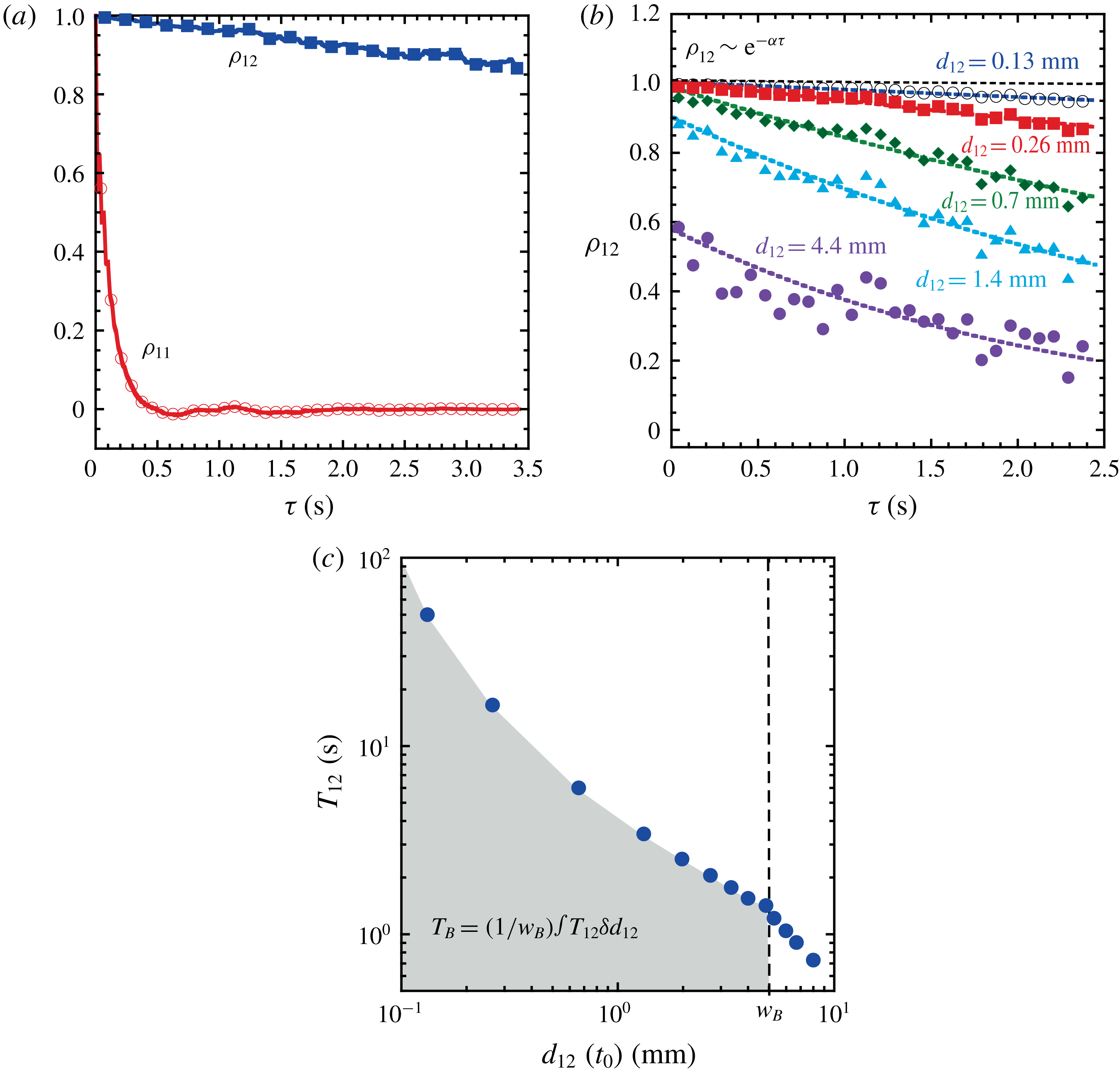
Figure 7(a) shows that the memory of a single particle is quite different from that of two particles very close to each other (
 $d_{12}(t_{0})\ll L_{f}$
). In that case, a single particle forgets about its initial motion on a time scale
 $T_{L}$
that is 250 times smaller than
 $T_{12}$
. To better understand this strong effect, we investigate the dependence of
 $\unicode[STIX]{x1D70C}_{12}$
on the initial separation distance
 $d_{12}$
at a fixed flow energy
 $U^{2}$
and fixed forcing scale
 $L_{f}\approx 4.4$
mm. As seen in figure 7(b), the larger the initial separation, the faster the decorrelation in the motion of the particle pair. Moreover, the cross-correlation function can be fitted by an exponentially decaying function
 $\unicode[STIX]{x1D70C}_{12}\approx A\exp (-\unicode[STIX]{x1D6FC}\unicode[STIX]{x1D70F})$
, where the parameters
 $A$
and
 $\unicode[STIX]{x1D6FC}$
are both decreasing functions of the initial separation
 $d_{12}(t_{0})$
.
The dependence of
 $\unicode[STIX]{x1D70C}_{12}$
on the initial separation
 $d_{12}(t_{0})$
is directly reflected in the behaviour of
 $T_{12}$
as a function of
 $d_{12}(t_{0})$
, which is shown in figure 7(c). The time scale
 $T_{12}$
decreases with the increase in the initial separation. The values taken by
 $T_{12}$
for small separation
 $d_{12}(t_{0})<L_{f}$
are much larger than
 $T_{L}$
. A clear kink can be seen at a length scale called
 $w_{B}$
beyond which
 $T_{12}$
decreases strongly to 0. The measurements give
 $w_{B}\approx 5~\text{mm}$
which is close to the forcing scale
 $L_{f}\approx 4.4~\text{mm}$
. These results suggest that a large number of fluid particles travel together forming trajectory bundles whose characteristic width is close to
 $w_{B}$
and which sustain a coherent motion for a long time.
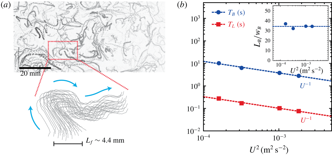
Such a bundle of trajectories is shown in figure 8(a). Figure 7(a) shows that the wave-driven turbulence possesses both random walk features with a short time scale
 $T_{L}$
dominating the single-particle statistics (Xia et al.
Reference Xia, Francois, Punzmann and Shats2013), and highly correlated features with a much longer time scale
 $T_{12}$
clearly identified by the cross-correlation function. Figure 8(a) illustrates that the random walk is executed by trajectory bundles as a whole, rather than by an ensemble of uncorrelated trajectories.
A bundle correlation time
 $T_{B}$
can be derived by integrating the cross-correlation time
 $T_{12}$
with respect to the initial separation
 $d_{12}(t_{0})$
, as
 $T_{B}=(1/w_{B})\int _{0}^{w_{B}}T_{12}\unicode[STIX]{x2202}d_{12}$
(see figure 7
c). Both the autocorrelation time
 $T_{L}$
and cross-correlation time
 $T_{B}$
are shown in figure 8(b) as a function of the flow kinetic energy. Although the lifetime of a bundle
 $T_{B}$
is much longer than the single-particle time scale
 $T_{L}$
, figure 8 shows that the two time scales are correlated. Indeed,
 $T_{B}$
and
 $T_{L}$
are both inversely proportional to the r.m.s. of the velocity fluctuations
 $U$
:
 $T_{B}\sim T_{L}\sim 1/U$
. This suggests that the same underlying process governs the randomisation of the bundle motion and its disappearance. The long lifetime of the bundle (
 $T_{B}\approx 30\times T_{L}$
) reflects the fact that the bundle length is much larger than its width (see figure 8
a). The bundle length is estimated as
 $L_{B}=U\times T_{B}$
. The resulting lengths of the bundles are shown as an inset in figure 8(b);
 $L_{B}$
is roughly 30 times the width of the bundle
 $w_{B}$
.
(a) A typical bundle of trajectories (lower panel) measured in wave-driven turbulence. The upper panel shows particle streaks measured in the turbulent flow (with
 $L_{f}=4.4~\text{mm}$
and
 $U^{2}=1\times 10^{-3}~\text{m}^{2}~\text{s}^{-2}$
). The bundle is tracked using PTV for a time interval
 $\text{d}t\approx 8T_{L}$
; the blue arrows indicate the bundle dynamics. (b) The autocorrelation
 $T_{L}$
and cross-correlation
 $T_{B}$
time of the flow velocity fluctuations, as functions of the kinetic energy of the flow. (Parameters:
 $f_{s}=60~\text{Hz}$
,
 $L_{f}\approx 4.4~\text{mm}$
.) Inset: the ratio of the length to the width of the coherent bundles.

3.5 Disc–turbulence coupling
3.5.1 Temporal memory
The results of the previous section help one to better understand the transition observed in figure 6(b) for the dependence of the characteristic time
 $T_{disc}$
on the flow energy
 $U^{2}$
. The flow analysis indicates that the building blocks of the wave-driven turbulent flow are coherent bundles, whose width is limited by the characteristic scale
 $w_{B}\approx L_{f}$
. It is reasonable to think that a small floater
 $r_{p}<w_{B}$
is carried and influenced at each instant by a unique bundle. It suggests a direct relationship between the disc memory time
 $T_{disc}$
and the bundle correlation time
 $T_{B}$
. In that respect, the functional dependence
 $T_{B}\sim 1/U$
is consistent with the scaling
 $T_{disc}\sim 1/U$
shown in figure 6(b) for a small disc (
 $r_{p}<L_{f}$
). In this regime, the diffusion coefficient of the discs depends on the flow energy according to
 $D=U^{2}T_{disc}\sim U$
(figure 5
c). This scaling is actually identical to that measured in the case of fluid tracers as reported in Xia et al. (Reference Xia, Francois, Punzmann and Shats2013).
In contrast, a large floater interacts continuously with many bundles. The interaction of the floater with this bath of fluid bundles results in a constant memory time
 $T_{disc}$
and a diffusion coefficient given by
 $D\sim U^{2}T_{disc}\sim U^{2}$
. This scaling suggests a fluctuation–dissipation-like relation, which we will discuss in the last section of the paper.
3.5.2 Floating discs as filters of the fluid dynamics
In figure 4(b), a clear transition in the velocity variance
 $V_{p}^{2}$
of the disc as a function of the size
 $r_{p}$
has been identified. This transition is related to a modification of the momentum transfer between the disc and the turbulent flow. In this section, we explore further this feature of the disc–turbulence coupling. An intuitive phenomenology to describe this coupling relies on the idea that the dynamics of finite-size discs reflects a filtered response of the turbulent fluid motion. In other words, the floating discs are filters of the fluid dynamics and the spatio-temporal parameters of these filters are the time scale
 $T_{disc}$
and the disc radius
 $r_{p}$
.
In the following, we compute the average of the fluid velocity vector
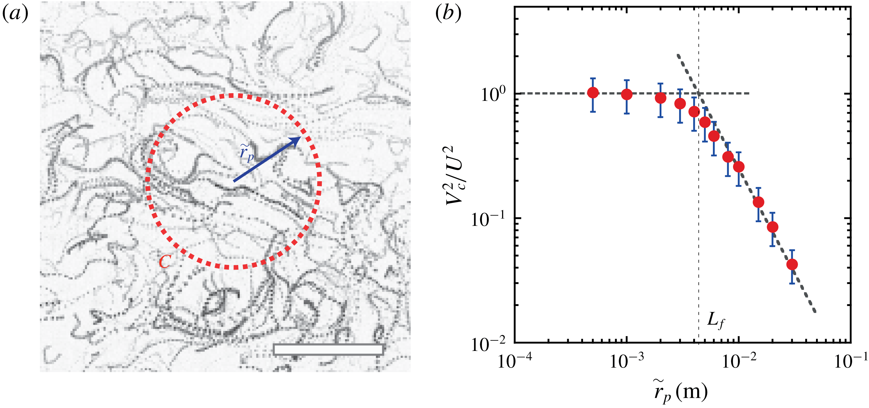
 $\boldsymbol{u}=(u_{x},u_{y})$
on a virtual circular contour placed in an unperturbed turbulent flow (i.e. a flow in the absence of the physical floating disc). Our approach is illustrated in figure 9(a). The figure shows fluid particle streaks and the red dotted circle indicates the contour
 $C$
on which we compute the square of the contour averaged velocity,
 $$\begin{eqnarray}V_{C}^{2}(r_{p})=\langle \overline{u_{x}}\rangle ^{2}+\langle \overline{u_{y}}\rangle ^{2},\end{eqnarray}$$
where the spatial averaging is
 $\overline{u_{i}}=(1/(2\unicode[STIX]{x03C0}r_{p}))\oint _{C}u_{i}r_{p}\,\text{d}\unicode[STIX]{x1D703}$
and
 $\langle ~\rangle$
denotes temporal over
 $T_{disc}$
and statistical averaging. It is important to note that
 $V_{C}^{2}$
is different from a simple averaging of squared velocity component. For instance, in the absence of mean flow
 $V_{C}^{2}$
tends to 0 for large radius
 $r_{p}$
because the spatial averaging is performed first.
(a) Schematic illustrating the measurement of the stress
 $\unicode[STIX]{x1D70E}_{r}$
on the virtual circular contour
 $C$
(red dotted circle) of radius
 $\tilde{r}_{p}$
. The background shows fluid particle streaks measured in the turbulent flow. Scale bar is
 $20~\text{mm}$
. (b) Filtered flow energy
 $V_{C}^{2}$
normalised by the flow energy
 $U^{2}$
as a function of
 $\tilde{r}_{p}$
. The squared velocity
 $V_{C}^{2}$
is averaged along the circular contour
 $C$
and over time
 $T_{disc}$
. The turbulent flow energy and the forcing scale are fixed:
 $U^{2}=1\times 10^{-3}~\text{m}^{2}~\text{s}^{-2}$
,
 $L_{f}\approx 4.4~\text{mm}$
.

We measure
 $V_{C}^{2}$
for different radii
 $\tilde{r}_{p}$
of the virtual contour. Figure 9(b) shows
 $V_{C}^{2}/U^{2}$
as a function of
 $\tilde{r}_{p}$
for a fixed flow energy
 $U^{2}$
. The filtered energy
 $V_{C}^{2}$
decreases when
 $\tilde{r}_{p}$
increases. A transition occurs at
 $\tilde{r}_{p}\approx L_{f}$
which is close to that observed for
 $V_{p}^{2}/U^{2}$
in figure 4(b). These data show two regimes in the spatio-temporal filtering of the fluid velocity along a circular contour. We propose a simple interpretation of these two regimes. As long as
 $\tilde{r}_{p}$
is varied in a range of size smaller than
 $L_{f}$
, a circular contour is most likely crossed by a single bundle; consequently the filtered velocity depends weakly on
 $\tilde{r}_{p}$
. This is consistent with the picture of a small disc advected by a unique bundle. In contrast, a larger contour
 $\tilde{r}_{p}>L_{f}$
intersects many bundles and the larger
 $\tilde{r}_{p}$
, the more independent bundles are crossing the contour. Consequently
 $V_{C}^{2}$
strongly decreases with
 $\tilde{r}_{p}$
, a feature similar to what is observed for large discs in figure 4(b).
We note that this similarity is quite remarkable because
 $V_{C}^{2}$
and
 $V_{p}^{2}$
are different quantities: the filtered velocity
 $V_{C}^{2}$
is an Eulerian quantity while
 $V_{p}^{2}$
is a Lagrangian quantity. The relationship between the Eulerian and Lagrangian description of turbulence remains an outstanding question in the theory of turbulence (Monin & Yaglom Reference Monin and A. M.1975). In this study, the knowledge of the fine structure of wave-driven turbulence helps to create a tantalising bridge between the size dependence of the Eulerian average velocity
 $V_{C}^{2}$
and the Lagrangian velocity
 $V_{p}^{2}$
.
4 Discussion
In these experiments, we have studied the turbulent diffusion coefficient
 $D$
of floating objects placed in wave-driven turbulence. Two regimes have been identified for the dependence of the diffusion coefficient on the size
 $r_{p}$
of the floating object. The diffusion coefficient can be written as
 $D\sim V_{p}^{2}T_{p}\sim CU^{2}T_{p}$
and our results allow a better understanding of the trends in function of the radius
 $r_{p}$
observed in figure 3; indeed,
(i) when
 $r<L_{f}$
we measured that
$C\sim r^{-0.35}$
and
$T_{p}\sim \text{const.}\sim L_{f}/U$
(see figures 4
b and 6
a), hence,
$D\sim r^{-0.35}$
; and
(ii) when
$r>L_{f}$
we measured that
$C\sim r^{-2}$
and
$T_{p}\sim r$
(see figures 4
b and 6
a), hence,
$D\sim r^{-1}$
.


We test these relations in figure 10(a) which shows that all our data can be collapsed onto a master curve by normalising the diffusion coefficient
 $D$
by the product of the flow velocity variance
 $U^{2}$
and the integral time scale
 $T_{p}$
and plotting it versus the ratio
 $C=V_{p}^{2}/U^{2}$
.
Though our system is macroscopic, analogies can be drawn with phenomena observed at the microscopic scale. Such analogies are often fruitful, as mentioned in the original paper of Taylor on turbulent diffusion (Taylor Reference Taylor1921). For instance, fluctuation–dissipation relations play a central role in statistical physics, and one famous instance is the Stokes–Einstein relation for diffusion of Brownian spherical particles of radius
 $r$
. This relation predicts that the diffusion coefficient
 $D$
increases linearly with the thermal energy
 $kT$
and is inversely proportional to the radius
 $r$
, namely
 $D=kT/(6\unicode[STIX]{x03C0}\unicode[STIX]{x1D702}r)$
, where
 $\unicode[STIX]{x1D702}$
is the fluid viscosity.
In the macroscopic turbulent flow described here, the behaviour of the large discs
 $r_{p}>L_{f}$
is interesting. Indeed the diffusion coefficient
 $D=V_{p}^{2}T_{disc}$
of large discs is inversely proportional to their radius
 $r_{p}$
(see figure 3); moreover it has been shown that their kinetic energy
 $M_{p}V_{p}^{2}$
is directly proportional to an effective flow kinetic energy,
 $M_{p}V_{p}^{2}=\unicode[STIX]{x1D707}U^{2}$
, where
 $\unicode[STIX]{x1D707}$
is a constant (see the inset of figure 4
b). These two features allow us to write a simple relation between
 $D$
and the effective flow energy, namely
 $D=\unicode[STIX]{x1D707}U^{2}/(\unicode[STIX]{x1D702}_{s}r_{p})$
, where
 $\unicode[STIX]{x1D702}_{s}$
is a constant that has the dimension of viscosity. Figure 10(b) shows the behaviour of the dimensionless number
 $D/(\unicode[STIX]{x1D707}U^{2}/(\unicode[STIX]{x1D702}r_{p}))$
(
 $\unicode[STIX]{x1D702}$
is the viscosity of water) as a function of the ratio
 $C=V_{p}^{2}/U^{2}$
. It confirms the existence of a relation analogous to the Stokes–Einstein relation for low values of
 $C$
corresponding to large floating objects. Similar relations have recently been studied in the Faraday wave system (Welch, Liebman-Pelaez & Corwin Reference Welch, Liebman-Pelaez and Corwin2016). It would be interesting to see how they can be connected to other properties of the liquid–gas interface perturbed by waves (Domino et al.
Reference Domino, Tarpin, Patinet and Eddi2016). The behaviour of the small discs
 $r_{p}<L_{f}$
does not allow for such a simple relation to be written but instead reflects the memory of this strongly out-of-equilibrium flow via diffusion coefficients that are proportional the flow r.m.s. velocity
 $U$
.
It is interesting to note that the coupling between the flow fabric with large floating objects can give rise to interesting phenomena if the object has an asymmetric shape (Francois et al. Reference Francois, Xia, Punzmann and Shats2018). Recently, it has been demonstrated that such objects are able to extract energy from 2D turbulence and this offers methods to create turbulence-driven turbines or self-propelled vehicles (Francois et al. Reference Francois, Xia, Punzmann and Shats2018; Yang et al. Reference Yang, Davoodianidalik, Xia, Punzmann, Shats and Francois2019).
(a) Non-dimensional diffusion coefficient
 $D/U^{2}T_{p}$
versus the ratio
 $C=V_{p}^{2}/U^{2}$
. The diffusion coefficient of the floating object
 $D$
is normalised by the product of the flow velocity variance
 $U^{2}$
and the corresponding integral time scale
 $T_{p}$
. (b) Non-dimensional diffusion coefficient
 $D=\unicode[STIX]{x1D707}U^{2}/(\unicode[STIX]{x1D702}r_{p})$
versus the ratio
 $C=V_{p}^{2}/U^{2}$
. The vertical dashed line indicates the transition observed at
 $r_{p}=L_{f}$
in the dependence of
 $C$
on
 $r_{p}$
shown in figure 4(b). (Experimental parameters:
 $f_{s}=60~\text{Hz}$
,
 $L_{f}\approx 4.4~\text{mm}$
.)

5 Conclusions
Summarising, here we show a connection between the turbulent diffusion of inertial particles and the Lagrangian structure of 2D turbulence. We demonstrate that anisotropic river-like structures are the underlying fabric of 2D turbulence generated by steep waves at the liquid surface. Depending on their size, floating discs interact differently with these transient river-like structures. While large objects interact with many bundles, small objects can only be influenced by a single bundle at a time. These two distinct behaviours are directly reflected by how the diffusion coefficient depends on both the object size and the flow kinetic energy. This finding opens ways of engineering a non-equilibrium liquid interface with tunable diffusion coefficient (Welch et al. Reference Welch, Liebman-Pelaez and Corwin2016; Francois et al. Reference Francois, Xia, Punzmann, Fontana and Shats2017). In the case of a liquid surface perturbed by Faraday waves, our results offer methods to externally tune the diffusion coefficient of a floating object by changing the amplitude or the frequency of the vertical oscillation.
Acknowledgements
This work was supported by the Australian Research Council’s Discovery Projects funding scheme (DP150103468 and DP160100863). H.X. acknowledges support from the Australian Research Council’s Future Fellowship (FT140100067). N.F. acknowledges support by the Australian Research Council’s DECRA award (DE160100742). The authors thank K. Szewc for developing the analysis code of the PIV trajectories. We thank the anonymous referees for their constructive comments.