1. Introduction
The transition from laminar to turbulent boundary layer occurs through the spatial sporadic onset of turbulence. These sporadic regions of turbulence superimposed over a laminar boundary layer are called ‘turbulent spots’. The turbulent spots are convected downstream from the location of their inception during which they grow in size and merge to result in a fully developed turbulent boundary layer (Emmons Reference Emmons1951). The boundary layer exhibits an intermittent nature, alternating between laminar and turbulent states, during convection and growth of the turbulent spots. A formal mathematical definition of intermittency associated with transitional boundary layers was proposed by Narasimha (Reference Narasimha1957). A review of earlier works on turbulent spots in subsonic and low supersonic flows can be found in Narasimha (Reference Narasimha1985). A general outline and recommendations for experimental measurement of intermittency was given by Hedley & Keffer (Reference Hedley and Keffer1974) and Narasimha (Reference Narasimha1985). Experimental measurements on the intermittent nature of compressible high-speed transitional boundary layers have been usually carried out by using thermal sensors such as thin film sensors or thermocouples. The intermittency distribution on a compressible boundary layer developed over a cone closely followed the incompressible distribution (Owen & Horstman Reference Owen and Horstman1972). Turbulent spots developed on a zero pressure gradient and a favourable pressure gradient planar boundary layer were characterised in terms of their leading- and trailing-edge speeds for a range of free-stream Mach numbers with a conclusion that a favourable pressure gradient led to an increase in trailing-edge speeds of the spots while the leading-edge speeds remained unaffected (Clark, Jones & LaGraff Reference Clark, Jones and LaGraff1994). Surface heat transfer measurements were used to calculate speeds and length scales associated with turbulent spots developed on a cylinder with a blunt spherical nose (Fiala et al. Reference Fiala, Hillier, Mallinson and Wijesinghe2006). Speeds associated with turbulent spots developed on a
 $5^{\circ }$
cone under high enthalpy hypersonic flow were calculated from experimental measurements of heat transfer (Jewell et al. Reference Jewell, Parziale, Leyva and Shepherd2012). Mee & Tanguy (Reference Mee and Tanguy2015) established a logarithmic linear corelation for the spot initiation rate with unit Reynolds number for planar boundary layers. The efficacy of methods for calculating intermittency other than surface heat transfer measurements, such as density and pressure fluctuation data, was studied on a hypersonic boundary layer formed over a flat plate by Lunte and Schülien (Reference Lunte and Schülein2025). The turbulent spots in hypersonic transitional boundary layers have also been studied numerically using direct numerical simulations (Krishnan & Sandham Reference Krishnan and Sandham2006; Hader & Fasel Reference Hader and Fasel2019). The numerical simulations showed turbulent spots to have an upstream-pointed arrowhead shape with a leading-edge overhang, followed by a turbulent core and a calmed region at the rear interface.
Although the basic structure of a turbulent spot in a hypersonic boundary layer is well understood from the works described in this section, data pertaining to the characteristics associated with the spots such as convection speeds, length scales and generation rate are scarce in the open literature. Existing studies have explored turbulent spots on a particular test model and a comparison between the spots developed on different test models under similar free-stream conditions has not been reported in the open literature. The present work was conducted with a motivation to address this lacunae in the existing work since it can provide insights which can be used to explain subtle differences in transitional boundary layer characteristics across different test models. The objectives of the present work include characterising the turbulent spots developed in a planar and an axisymmetric boundary layer. The planar boundary layer was developed on a flat plate and the axisymmetric boundary layer was developed on a right angled cone. The test models were kept under similar free-stream conditions such that the boundary layer edge Mach number and unit Reynolds number on both the test models remained same within uncertainty limits.
Figure depicting schematic of HST4.

2. Experimental details
2.1. Hypersonic shock tunnel 4 (HST4) facility
The experiments in the present work were conducted in Hypersonic Shock Tunnel 4 (HST4) of the Laboratory for Hypersonic and Shockwaves Research at Indian Institute of Science. The HST4 is a pressure-driven shock tunnel equipped with an axisymmetric contour nozzle capable of generating hypersonic flow in the test section for a useful test duration of
 ${3.5}\,\textrm {ms}$
. A schematic of the facility is shown in figure 1. In the present work HST4 is operated to result in a free-stream Mach number of
 $5.8\pm 0.1$
. The free-stream unit Reynolds number varied in the range of
 $(3.0-6.0)\times 10^{6}$
m−1. Further details on the facility can be found in Bajpai and Jagadeesh (Reference Bajpai and Gopalan2023).
2.2. Models, test conditions and instrumentation
A flat plate with a sharp leading edge and a right angled cone with a sharp tip have been used as test models in the present work. The length of the flat plate and the axial length of the cone was
 ${800.0}\,\textrm {mm}$
. The test models were fabricated with duralumin with stainless steel leading edge and cone tip. The surface roughness of the test models was maintained at N10 ISO grade and the mating surfaces had a tolerance of
 $50\pm 10\,{\unicode{x03BC}}$
m. Both the leading edge of the flat plate and the tip of cone were machined to a sharpness of
 $80\pm 10\, {\unicode{x03BC}}$
m. The test models were equipped with 20 platinum thin film sensors for wall heat transfer measurements. The heat transfer measurement is used to ascertain the state of the boundary layer at a given spatial and temporal location. The distance between the thin film sensors varied along the length of the test model (from
 ${10.0}\,\textrm {}$
to
 ${70.0}\,\textrm {mm}$
) such that the sensors can monitor heat transfer levels in all the three states of the boundary layer, namely laminar, transitional and turbulent. The output from the heat transfer sensors was acquired at
 ${1.0}\,\textrm {MSas}^{-1}$
with a NI PXI 6133 DAQ. Figure 2 shows the schematic of the test models along with the typical placement of thin film sensors used in the present study.
Figure depicting schematics of flat plate and cone used in present work.

Similar free-stream conditions were maintained over both test models for various cases considered in the present work. The boundary layer edge conditions over both the test models were calculated using inviscid relations. In these calculations, the specific heat at constant pressure was held constant at
 ${1.005}\,\rm kJ\,kg^{-1}$
. The dynamic viscosity varied with temperature following Sutherland’s law with reference viscosity taken as
 $1.716\times 10^{-5}$
kg ms−1, reference temperature taken as
 ${273.15}\,\textrm {K}$
and Sutherland temperature taken as
 ${110.4}\,\textrm {K}$
. The boundary layer edge conditions over the cone are governed by the semi-angle of the cone, which is
 $12^{\circ }$
. The flat plate in the present work was kept at an angle of attack of
 $10^{\circ }\pm 0.5^{\circ }$
so that the edge Mach number (
 $M_{e}$
) and edge unit Reynolds number (
 $\textit{Re}_{e}$
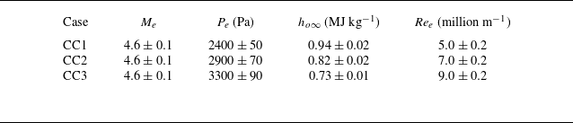
) over the plate can match with corresponding edge conditions of the cone. Tables 1 and 2 show the boundary layer edge conditions maintained over the flat plate and cone, respectively, in the experiments.
Typical boundary layer edge conditions for flat plate.

Typical boundary layer edge conditions for cone (no transition onset observed for CC1).

3. Results and discussion
3.1. Heat transfer and intermittency calculations
Figure 3 shows the typical heat transfer time history acquired from a thin film sensor and its association with convection of a turbulent spot over the sensor location. The deviation of heat transfer from theoretical laminar levels marks the passage of the leading edge of the spot over the sensor location and the return of heat transfer to the theoretical laminar levels marks the passage of trailing edge of the spot. Figure 3 shows that the heat transfer values deviate from the theoretical laminar level between
 $3.8$
and
 $4.3$
ms due to the passage of a turbulent spot over the sensor. Heat transfer time histories were used to quantify intermittency (
 $\gamma$
), which is a measure of the fraction of the boundary layer that has transitioned into fully turbulent state at a given location on a test model.
(a) Typical raw signal and post-processed heat transfer time history obtained through a thin film sensor. (b) Zoomed in view of heat transfer time history and its association with various features of a typical turbulent spot; ( ) and (
 ) lines show theoretical laminar and turbulent heat transfer levels, respectively, and
 $U_{\textit{le}}$
and
 $U_{\textit{te}}$
are the speeds associated with the leading and trailing edges of the spot, respectively. Here,
 $Q$
is the wall heat flux rate.

(a) Work flow involved in intermittency calculation from heat transfer time history. Here,
 $D_{i}$
and
 $C_{i}$
are the detector function and criterion function for the
 $i{\rm th}$
data point, respectively, and
 $\gamma _{e}$
is the intermittency calculated from experimental measurement of surface heat transfer. (b,c,d,e) Typical heat transfer time histories along with criterion function (
 ) and intermittency (
 ) time histories from sensors placed in transitional boundary layers developed over the flat plate (d,e) and cone (b,c).

The procedure for the calculation of the intermittency for both the flat plate and the cone is the same and is outlined in figure 4(a). The procedure closely follows the methodology outlined in Clark et al. (Reference Clark, Jones and LaGraff1994) and Mee & Goyne (Reference Mee and Goyne1996). The definition of detector function (
 $D_{i}$
) has been modified in the present work and a comparison between earlier definitions of the detector function and the present definition is outlined in Appendix A. In the present work, the detector function expression scales the square of the time derivative of the heat transfer using the maximum and mean values of the heat transfer registered by a heat transfer sensor. The temporal derivative of heat transfer was calculated using a second-order finite difference method. From the detector function, a criterion function (
 $C_{i}$
) was defined, which is an exponentially weighted (
 $\omega _{j}$
) centred moving average based on the sampling interval (
 $h$
) and smoothing period (
 $\tau =20\, {\unicode{x03BC}} \textrm{s}$
). The purpose of the criterion function is to sensitise the detector function to efficiently distinguish between turbulent and non-turbulent regions of the boundary layer. The criterion function is normalised by its maximum value obtained from the data of all the sensors for a particular experiment. The intermittency is then set to
 $1$
if the criterion function crosses a certain threshold (
 $C_{\textit{th}}$
), otherwise it is set to
 $0$
. In the present work, the value of
 $C_{\textit{th}}$
is taken as
 $0.1$
times the maximum value of the normalised criterion function obtained in a particular experimental run. The intermittency is also set to
 $1.0$
if the heat transfer level at a particular sensor location crosses
 $0.8$
times the theoretical turbulent heat transfer levels calculated from Eckert’s method.
A typical result from the application of this work flow for the calculation of the intermittency time history from the heat transfer time history is shown in figure 4(b,c,d,e). More details on the intermittency calculation methodology followed in the present work can be found in Appendix A. From figure 4(b,c,d,e) it is clear that the methodology followed in the present work efficiently captures the intermittency associated with the transitional boundary layers encountered in the present work. The average of the intermittency time history results in the intermittency at a sensor location. A spatial distribution of intermittency is thus obtained, as shown in figure 5. In figure 5, the spatial distribution of intermittency obtained through all the experiments conducted in the present campaign is compared with the universal intermittency distribution on the flat plate and cone. The universal intermittency distribution for flat plate (
 $\gamma _{\textit{plate}}$
) and cone (
 $\gamma _{\textit{cone}}$
) is calculated based on the following analytical relations (Narasimha Reference Narasimha1985):
 \begin{equation} \gamma _{\textit{plate}} = 1.0 - \textit{exp}\left [-(x-x_{tr})^{2}\frac {n\sigma }{U_{e}}\right ]\!, \end{equation}
 \begin{equation} \gamma _{\textit{cone}} = 1.0 - \textit{exp}\left [-\frac {n\sigma }{U_{e}}x_{tr}\left (ln\frac {x}{x_{tr}}\right )(x-x_{tr})\right ]\!. \end{equation}
In (3.1) and (3.2),
 $n$
refers to the spot generation parameter,
 $U_{e}$
refers to the boundary layer edge speed,
 $x_{tr}$
refers to the transition onset location and
 $\sigma$
denotes the spot growth parameter defined by (3.3) (Vinod & Govindarajan Reference Vinod and Govindarajan2004)
 \begin{equation} \sigma = \left [\frac {1}{U_{\textit{te}}}-\frac {1}{U_{\textit{le}}}\right ]U_{e} \textit{tan}{\alpha }. \end{equation}
In (3.3),
 $\alpha$
is the spot spread angle defined as a function of the boundary layer edge Mach number in (3.4) (Doorly & Smith Reference Doorly and Smith1992). Experimental calculation of the leading (
 $U_{\textit{le}}$
) and trailing (
 $U_{\textit{te}}$
) edge speeds is discussed in the next section
 \begin{equation} \alpha = 3^{-3/2}2^{1/2}M_{e}^{-1}. \end{equation}
Figure 5 clearly shows that the boundary layer on a flat plate experiences an early onset of transition when compared with the cone under similar boundary layer edge conditions. It also clearly indicates that, for the same unit Reynolds number, the transitional boundary layer length on a flat plate is shorter than the one developed on a cone.
Spatial distribution of intermittency along the length of the (a) flat plate and (b) cone for all the experimental runs; ( ) line represents universal intermittency for one of the shots for every experimental condition.

3.2. Turbulent spot speeds, streamwise length scales and generation rates
Figure 6(a) shows typical convection of a turbulent spot identified by using the heat transfer and intermittency time histories of three heat transfer sensors placed over the surface of cone. The leading edge and trailing edge of the turbulent spot is identified by the intermittency switch. A similar technique was used in the case of the flat plate as well. The distance between the sensors and the time taken by the leading and trailing edges of the spot to traverse the distance between the sensors is known. The speeds associated with the leading edge (
 $U_{\textit{le}}$
) and trailing edge (
 $U_{\textit{te}}$
) of the turbulent spots can be calculated. In the present work, 19 distinct turbulent spots were identified in all the experiments for the flat plate and 16 distinct spots were identified for the cone. For each one of the spots, a distance time trace for the leading and trailing edges of the spot was plotted, as shown in figure 6(b), the slope of which is the corresponding speeds of the spot. The distance time trace, for each turbulent spot, was plotted for its convection across 2–5 heat transfer sensors. The calculated leading- and trailing-edge speeds were normalised with the boundary layer edge speed to result in the normalised leading (
 $C_{\textit{le}}$
) and trailing (
 $C_{\textit{te}}$
) edge speeds associated with turbulent spots for both the flat plate and the cone, as shown in figure 7.
(a) Heat transfer and intermittency time history capturing the convection of a turbulent spot over the cone. The first two sensors are 70 mm apart and the second and third sensors are 60 mm apart. The leading edge ( ) and trailing edge (
 ) of the spot are identified using the intermittency levels. Intermittency over each sensor location is shown by (
 ). (b) Distance vs time trace of leading and trailing edges of a typical spot developed on the cone and flat plate. The leading- and trailing-edge speeds are calculated from the slope of these traces, shown by (
 ) for the cone and (
 ) for the flat plate.

From figure 7 it is evident that, for a given boundary layer edge speed, the leading edge of the turbulent spots developed on the cone and flat plate are convected at comparable speeds, while the trailing edge of the spots on the flat plate moves with a slower speed than those developed on the cone. It is evident, from the spot velocity data, that the spots developed in a planar boundary layer have a larger streamwise growth rates than their axisymmetric counterpart. A first-order approximation of the length of the turbulent spots can further elucidate this aspect. The maximum and minimum streamwise length scales (
 $l_{\textit{max}}$
and
 $l_{\textit{min}}$
) associated with the turbulent spots can be estimated by (3.5) and (3.6) (Fiala et al. Reference Fiala, Hillier, Mallinson and Wijesinghe2006). In (3.5) and (3.6) and subsequent equations,
 $t_{\textit{te}}$
and
 $t_{\textit{le}}$
are the time stamps where the trailing edge and the leading edge of the spot cross the sensor location
 \begin{equation} l_{\textit{max}}=U_{\textit{le}}(t_{\textit{te}}-t_{\textit{le}}), \end{equation}
 \begin{equation} l_{\textit{min}}=U_{\textit{te}}(t_{\textit{te}}-t_{\textit{le}}). \end{equation}
The convection speed of a turbulent spot varies along its length and in the present work it is assumed that the spot convects at a speed (
 $U_{sc}$
) which is the mean of the leading-edge and trailing-edge speeds ((3.7)). This assumption leads to a first-order approximation of the spot streamwise length scales, given by (3.8), which is reasonable enough to compare streamwise growth rate of turbulent spots generated in the flat plate and cone
 \begin{equation} U_{sc}=0.5(U_{\textit{le}}+U_{\textit{te}}), \end{equation}
 \begin{equation} l_{ts} \approx U_{sc}(t_{\textit{te}}-t_{\textit{le}}). \end{equation}
Normalised spot leading-edge ( ) and trailing-edge (
 ) speeds of turbulent spots identified in all the experiments conducted over (a) the flat plate and (b) the cone. In both the figures (
 ) and (
 ) show the lower and upper bounds of the 95 % confidence interval for normalised leading-edge and trailing-edge speeds, respectively.

Streamwise length scale estimates of turbulent spots identified from (3.8) at various sensor locations along the (a) flat plate’s surface and (b) cone’s surface. The ( ) line shows the linear fit to the spot length data with slope ranges indicated in the figure. The intersection of the (
 ) line with the x-axis shows an approximate location of the generation of the turbulent spots on a particular test model surface (Fiala et al. Reference Fiala, Hillier, Mallinson and Wijesinghe2006).

The streamwise length estimates obtained from (3.8) at various locations on the flat plate and cone are shown in figure 8. A quick comparison between figures 8(a) and 8(b) shows that turbulent spots generated on a flat plate experience a larger streamwise growth rate along the length of the plate owing to their slower trailing-edge speed when compared with the spots generated on the cone. This aspect is clearly elucidated in the schematic shown in figure 9(a). Here, the turbulent spot developed on a flat plate enlarges more when compared with the spot developed on the cone if both the spots traverse a similar length along the plate and cone. It is to be noted that the transitional boundary layer onset location and length are different for the plate and cone.
The spot generation rates in the present work have been calculated from (3.1) and (3.2). The right-hand side of both (3.1) and (3.2) is determined from experimental data with the procedure outlined in § 3.1. All the quantities on the left-hand side and right-hand side of both (3.1) and (3.2) have been calculated from present experiments, except for the spot generation rate parameter,
 $n$
. Hence the value of the spot generation parameter can be calculated by using the experimental outcomes of the present work and the same is shown in figure 9(b). For the same unit boundary layer edge Reynolds number, a higher number of turbulent spots are generated on a flat plate in comparison with a cone.
(a) Schematic depicting growth of a typical turbulent spot developed on a flat plate and the cone’s surface over the same longitudinal length. (b) Turbulent spot generation rate for the flat plate ( ) and the cone (
 ).

Earlier studies have shown that the transition onset Reynolds number for flat plate is lower than the one encountered in the case of a cone. Stability computations have also revealed that planar boundary layers are more receptive to the free-stream noise in comparison with the axisymmetric conical boundary layers (Chen, Malik & Beckwith Reference Chen, Malik and Beckwith1989; Schneider Reference Schneider2001). Hence, earlier transition onset is witnessed in a planar boundary layer in comparison with an axisymmetric boundary layer. A similar trend was found in the present study as well (figure 5). Furthermore, in the present study, the transitional boundary layer length over the flat plate was found to be shorter than its axisymmetric counterpart. The spot generation rate results reported here, in combination with the spot growth rate aspects, provide an explanation for the transitional boundary layer length being shorter in the flat plate when compared with the cone. For the same edge unit Reynolds number, a larger number of turbulent spots are generated on the flat plate in comparison with the cone (figure 9 b). After convecting through the same length a larger area would be occupied by the turbulent spots developed on the plate, owing to their higher longitudinal growth rate when compared with spots developed on the cone. The merging of turbulent spots to give rise to a fully developed turbulent boundary layer occurs over a shorter distance in the flat plate when compared with the cone owing to the aforementioned outcomes and observations. The experiments and analysis presented here provide a reason and explanation for the observations on boundary layer transition over a flat plate and cone reported in the earlier and present work.
4. Conclusions
The present work offers a unique comparison between transitional planar and axisymmetric boundary layers in terms of intermittency and turbulent spot characteristics such as spot leading- and trailing-edge speeds, growth of streamwise length scales and spot generation rates. Surface heat transfer measurement was carried out using platinum thin film sensors to ascertain the nature of the boundary layer developed on the test models. A methodology to calculate the intermittency from surface heat transfer measurements was outlined and a modified detector function definition was proposed and used in the present work. Characteristics of turbulent spots such as their leading-edge and trailing-edge speeds, length scales and spot generation rates were calculated for both the test modes. The leading edge of the turbulent spots developed on both the flat plate and cone convected at similar speeds which, in the present work, was found to be approximately 90 % of the boundary layer edge speed. It was found that the trailing edge of the spot developed in a planar boundary layer convected at a lower speed than the spot developed on an axisymmetric boundary layer. This difference in trailing-edge convection speed of turbulent spots affects their streamwise growth rate, with a higher growth rate for spots developed over a flat plate. It was also found that, for a similar boundary layer edge Reynolds number and Mach number, a higher number of turbulent spots are generated on planar boundary layers in comparison with axisymmetric boundary layers. These outcomes of the present work provide an explanation for the shorter transition lengths observed in the flat plate when compared with the cone.
Acknowledgements
The authors acknowledge funding from DRDO, New Delhi to carry out this work.
Declaration of interests
The authors declare no conflicts of interests.
Appendix A. Details of intermittency calculation procedure used in the present work
The heart of the intermittency calculation in the present and earlier works lies in the definition of the detector function (
 $D_{i}$
). The procedure in this work closely follows the recommendations from Hedley & Keffer (Reference Hedley and Keffer1974), Narasimha (Reference Narasimha1985) and the methodology from Clark et al. (Reference Clark, Jones and LaGraff1994) and Mee & Goyne (Reference Mee and Goyne1996). The general definition of the detector function used in the present as well as earlier works is shown in (A1)
 \begin{equation} D_{i} = m_{i}\!\left (\frac {{\rm d}Q}{{\rm d}t}\right )_{i}^{n} \end{equation}
In (A1),
 $m_{i}$
is a scaling parameter and
 $ {{\rm d}Q}/{{\rm d}t}$
is the time derivative of the heat transfer obtained from the sensor. Both Clark et al. (Reference Clark, Jones and LaGraff1994) and Mee & Goyne (Reference Mee and Goyne1996) have used n = 1 in the above formulation. Clark et al. (Reference Clark, Jones and LaGraff1994) used minimum and maximum values of the heat transfer obtained through a single gauge in the definition of
 $m_{i}$
. On the other hand, Mee & Goyne (Reference Mee and Goyne1996) have used theoretical laminar and turbulent heat transfer values in the definition of
 $m_{i}$
. The derivative of the heat transfer changes sign at critical points in the heat transfer time history, such as points of maximum heat transfer registered by the sensor. Since the detector function is to be designed to act as a switch of intermittency, a negative derivative is not desired. Mee & Goyne (Reference Mee and Goyne1996) overcame this problem by taking the absolute value of the heat transfer derivative. Clark et al. (Reference Clark, Jones and LaGraff1994) did not mention any such measures taken in their work but the authors in the present work assumed that the absolute value of the derivative was used in the formulation of the detector function in Clark et al. (Reference Clark, Jones and LaGraff1994). While comparing the present formulation of
 $D_{i}$
with that of Clark et al. (Reference Clark, Jones and LaGraff1994) both the original formulation and the formulation with our absolute value assumption are considered.
Hedley & Keffer (Reference Hedley and Keffer1974) recommended that the square of the derivative of a measured quantity is more efficient in distinguishing turbulent and non-turbulent regions of a boundary layer. Based on this recommendation, in the present work, n = 2 is used in (A1) to result in positive heat transfer derivative values. In (A1),
 $m_{i}$
is formulated by using the mean and maximum values of the heat transfer acquired from a heat transfer sensor. Furthermore, the absolute value of
 $m_{i}$
is taken in the present work. The formulation of the present detector function is shown in figure 4(a) and other formulations can be found in the aforementioned references and are not repeated here. All other aspects of the intermittency calculation such as sensitisation of the detector function to arrive at a criterion function and its normalisation are the same as in Clark et al. (Reference Clark, Jones and LaGraff1994), Mee & Goyne (Reference Mee and Goyne1996) and the present work but different smoothing periods (
 $\tau$
) and thresholds (
 $C_{\textit{th}}$
) have been used. The smoothing period (
 $\tau =20\,{\unicode{x03BC}}$
s for the present work) is used to efficiently distinguish between turbulent and non-turbulent parts of the boundary layer and was calculated based on the recommendations from Hedley & Keffer (Reference Hedley and Keffer1974). The smoothing period is a function of the boundary layer edge conditions and the sampling rate of data acquisition (
 $h$
). Clark et al. (Reference Clark, Jones and LaGraff1994) and Mee & Goyne (Reference Mee and Goyne1996) used a smoothing period of
 $10$
and
 $15\,{\unicode{x03BC}}$
s respectively according to their boundary layer edge conditions and data acquisition system. Another important parameter is the normalised threshold criterion function (
 $C_{\textit{th}}$
) and in the present work its value is taken as 10 % of the maximum normalised criterion (
 $C_{\textit{max}}$
) function obtained in a single experimental run. While Clark et al. (Reference Clark, Jones and LaGraff1994) did not mention their threshold criterion, Mee & Goyne (Reference Mee and Goyne1996) used 2.5 % of the
 $C_{\textit{max}}$
obtained in an experimental run as
 $C_{\textit{th}}$
.
A comparison among various criterion functions discussed here is shown in figure 10(a,b,c). The criterion functions are calculated for a typical heat transfer time history with an isolated turbulent spot. The smoothening time (
 $\tau$
) for all the formulations was taken as 20
 ${\unicode{x03BC}}$
s. From figure 10(b), it is evident that the original Clark et al. (Reference Clark, Jones and LaGraff1994) formulation does not capture the spot due to a sign change of the criterion function at a critical point in the heat transfer time history. Adopting the absolute value of the derivative in the same formulation improves the performance of the criterion function and it closely follows the formulation by Mee & Goyne (Reference Mee and Goyne1996). The theoretical laminar and turbulent heat transfer values used in the formulation by Mee & Goyne (Reference Mee and Goyne1996) were obtained using Eckert’s method. If Spalding’s method were used to obtain theoretical heat transfer levels, the intermittency calculated by Mee & Goyne (Reference Mee and Goyne1996) would decrease by 8 % and is not shown in figure 10(a,b,c) for clarity. Figure 10(a,b) shows that the formulation of the square of the heat transfer derivative, used in the present work, is better in capturing the turbulent spot while other formulations over-predict the intermittency by
 $38\,\%{-}50\,\%$
. Since the present formulation does not depend on theoretical estimates of the heat transfer, intermittency variations introduced due to such estimates are also avoided.
(a,b,c) Comparison of various formulations of the detector function for intermittency calculation on a typical heat transfer time history ( ). Clark-o represents original formulation of Clark et al. (Reference Clark, Jones and LaGraff1994) and Clark-m represents the same formulation with the absolute value of the heat transfer derivative. (d,e) Effect of change in smoothing period (
 $\tau$
) on normalised criterion function and intermittency (
 $\gamma _{e}$
). ( f) Effect of change in
 $C_{\textit{th}}$
on intermittency (
 $\gamma _{e}$
). Here,
 $C_{\textit{max}}$
is the maximum normalised criterion function obtained in an experimental test.

The effect of a change in the smoothing period on the criterion and intermittency function is shown in figure 10(d,e). The parameter
 $\tau$
was varied by 50 %–100 % from baseline
 $\tau =20\,{\unicode{x03BC}}$
s in this analysis, resulting in a intermittency variation of 15 %–30 % from the baseline value. It is clear that
 $\tau =20\,{\unicode{x03BC}}$
s is apt for the present work. The effect of a change in the criterion function threshold (
 $C_{\textit{th}}$
) on the intermittency calculation is also shown in figure 10( f). Here,
 $C_{\textit{th}}$
was also varied by 50 %–100 % from the baseline value which resulted in a
 $7.5\,\%$
change in intermittency from the baseline value. This shows that the intermittency calculated from the present work is more sensitive to the variation in
 $\tau$
than
 $C_{\textit{th}}$
.
A secondary criterion for intermittency switch was used in the present work to account for intermittency in fully developed turbulent boundary layers. The time derivative values in the detector function approach zero in fully developed laminar and turbulent boundary layers, as shown in figure 11. This is due to the fact that the heat transfer signals in both fully developed laminar and turbulent regions of the boundary layer have a relatively flatter signature parallel to the time axis. Hence a switch based on detector function alone would result in zero intermittency in fully developed laminar and turbulent boundary layers. While zero intermittency is correct for laminar boundary layers the same is not correct in turbulent boundary layers. Hence the need for a second intermittency criterion. In the context of identifying intermittency in fully developed turbulent boundary layers, the secondary criterion based on heat transfer should be high enough to not register any intermittency in a laminar boundary layer. In the present work, a switch based on
 $80\,\%$
of the theoretical turbulent heat transfer level was found to be apt. The threshold for this switch can be as high as the equivalent theoretical turbulent heat transfer levels.
Performance of the criterion function ( ) on fully developed (a) laminar (b) turbulent boundary layers. Heat transfer in the figure is shown by (
 ). Intermittency and theoretical heat transfer levels are shown by (
 ) and (
 ), respectively. The intermittency is 1 in (b) due to the secondary criterion.