1. INTRODUCTION
Since the Global Positioning System (GPS) signal is susceptible to interferences, land vehicle navigation systems cannot rely solely on GPS to be integrated with Strapdown Inertial Navigation Systems (SINS). An Odometer (OD) is a completely autonomous device to measure vehicle travelling distance/speed (Ding et al., Reference Ding, Li and Xiong2006). Therefore, SINS/OD integrated navigation systems may be considered as reliable schemes for vehicle navigation systems (Ding et al., Reference Ding, Li and Xiong2006; Yan, Reference Yan2006; Xiao et al., Reference Xiao, Wang, Cheng, Fu and Liu2012; Zhao et al., Reference Zhao, Miao and Shen2014). Zhao et al. (Reference Zhao, Miao and Shen2014) presented a high accuracy algorithm for a SINS/OD integrated navigation system. In the algorithm, two installation error angles and the OD scale factor error are augmented to be the system states, and the dimension of the system states increases to 18. That increases the computation amount and makes the performance of the Kalman filter degraded in real-time. Moreover, in SINS/OD integrated navigation systems, the variations of roadways or vehicle loads may cause changes to the OD scale factor errors, and the random noises of gyros and accelerometers tend to vary with time. Both of these may result in degradation or even divergence in the performance of the Kalman filter.
A unique procedure for estimating the dynamic states of a linear system in the presence of unknown constant biases was described by Friedland (Reference Friedland1969). This filter is called a Two-stage Kalman Filter (TKF). Ignagni (Reference Ignagni1981) proposed an alternate derivation of Friedland's result in which it was proved that TKF is equivalent to the Generalised Kalman Filter (GKF). Recently, TKF has been improved for the case that the biases are not only constant but also random (Ignagni, Reference Ignagni1990; Alouani et al., Reference Alouani, Xia, Rice and Blair1993; Keller and Darouach, Reference Keller and Darouach1997; Hsieh and Chen, Reference Hsieh and Chen1999; Ignagni, Reference Ignagni2000; Kanev and Verhaegen, Reference Kanev and Verhaegen2005; Hsieh, Reference Hsieh2010). However, TKF has the same drawbacks as a Kalman filter. Inaccuracy in system models may seriously degrade the performance of the filter. For example, TKF has high sensitivity to the stochastic information of noise and has no tracking ability to the suddenly changing bias. To overcome these drawbacks, Kim et al. (Reference Kim, Lee and Park2006; Reference Kim, Lee and Park2009) proposed the Adaptive Two-stage Kalman Filter (ATKF) and Adaptive Two-stage Extended Kalman Filter (ATEKF) in the presence of unknown random biases. But both of the filters used an incorrect condition that the innovations in a Bias-Free Estimator (BFE) are white noises with zero-mean.
In Adaptive Kalman filters (AKFs), adaptive algorithms are based on the important property that innovations in filters are white noise sequences with zero-mean (Xia et al., Reference Xia, Rao, Ying and Shen1994; Mohamed and Schwarz, Reference Mohamed and Schwarz1999; Hide et al., Reference Hide, Moore and Smith2003; Geng and Wang, Reference Geng and Wang2008; Shi et al., Reference Shi, Miao and Ni2010; Gao et al., Reference Gao, Miao and Ni2011). Xia et al. (Reference Xia, Rao, Ying and Shen1994) presented Multiple Adaptive factors Kalman Filter (MAKF) and Single Adaptive factor Kalman Filter (SAKF). Due to the complexity of computing multiple adaptive factors, MAKF is difficult to implement in real time. In contrast, SAKF is easier to apply. For complicated multivariable systems, the performance of MAKF is better than SAKF (Geng and Wang, Reference Geng and Wang2008; Gao et al., Reference Gao, Miao and Ni2011). Based on the special form of observation matrix, a class of MAKF algorithms were presented, in which the algorithms of computing adaptive factors were simple and easy to implement in real time (Geng and Wang, Reference Geng and Wang2008; Shi et al., Reference Shi, Miao and Ni2010; Gao et al., Reference Gao, Miao and Ni2011). But these algorithms cannot be used in the multivariable system with the general form of an observation matrix.
This paper proves that the innovation sequence of BFE in TKF is not zero-mean and the innovation of Bias Estimator (BE) is the same as the innovation of GKF which is equivalent to TKF. Therefore, it can be concluded that only the innovation of BE can be used in ATKF, which is a white noise sequence with zero-mean. Based on this conclusion, an ATKF algorithm for SINS/OD integrated navigation systems is proposed. Zhao et al. (Reference Zhao, Miao and Shen2014) presented a method of OD fault detection which is based on innovations. The method is used in the process of computing the multiple adaptive factors in the ATKF algorithm, which can avoid the complicated algorithm and constraint on the form of observation matrix.
2. PROBLEM FORMULATION
2.1. Coordinate Frames
Coordinate frames related in this paper are described as follows.
Navigation frame (n frame): is a local geographic coordinate frame. x n axis points towards east, and y n axis points towards north; z n axis is parallel to the upward vertical at the local position.
Calculated navigation frame (n′ frame): This is the navigation frame calculated by SINS.
Body frame (m frame): m frame is rigidly attached to the vehicle carrying the navigation system. x m axis is along the vehicle transverse axis; y m axis is along the vehicle longitudinal axis; z m axis is upward.
SINS frame (b frame): b frame is parallel to the strapdown inertial sensor axes, which should coincide with the m frame. Since the installation is not perfect, there are installation error angles between the b frame and the m frame.
2.2. Error Model of SINS/OD Integrated Navigation System
Zhao et al. (Reference Zhao, Miao and Shen2014) presented a novel error model of SINS/OD integrated navigation system based on velocity measurements in the b frame. A Kalman filter is designed for this model and a method of detecting OD fault is proposed. This error model is introduced as follows.
The state vector of this model with 18 dimensions is defined as:
 $$\eqalign{{\bi z} & = \left[ {\matrix{ {{\bi z}_{{\rm SINS}}^{\rm T} } & {{\bi z}_{{\rm OD}}^{\rm T} } \cr } } \right]^{\rm T}\cr & = \left[ {\matrix{ {{(\delta {\bi v}_{{\rm SINS}}^{\rm n} )}^{\rm T}} & {{({\bi \phi }^{\rm n})}^{\rm T}} & {{(\delta {\bi p})}^{\rm T}} & {{(\!{\nabla}^{\rm b})}^{\rm T}} & {{({\bi \varepsilon }^{\rm b})}^{\rm T}} & {\delta k} & {\delta \theta } & {\delta \psi } } } \right]^{\rm T}}$$
where
 ${\bi z}_{{\rm SINS}} $
is the state vector of SINS with 15 dimensions which consists of the velocity error vector
 $\delta {\bi v}_{{\rm SINS}}^{\rm n} $
, the attitude error vector
φ
n, the position error vector
 $\delta {\bi p}$
, the constant bias vector of accelerometers
 ${\nabla}^{\rm b}$
and the constant bias vector of gyros
ε
b,
 ${\bi z}_{{\rm OD}} $
is defined as the OD error state vector with three dimensions which is composed of the OD scale factor error δk, the pitch installation error of SINS δθ and the azimuth installation error of SINS δψ.
The OD scale factor error and the installation errors of SINS can be represented as
 $${\dot {\bi z}}_{{\rm OD}} = \left[ {\matrix{ {\delta \dot k} & {\delta \dot \theta} & {\delta \dot \psi} \cr}} \right]^{\rm T} = \left[ {\matrix{ 0 & 0 & 0 \cr}} \right]^{\rm T} $$
The state equation of SINS/OD integrated navigation system can be written as
 $$\eqalign{{\dot {\bi z}} & = {\bi \Phi} {{\bi z} + {\bi G}^{\prime}{\bi w}} \quad \cr & = \left[ {\matrix{ {{\bi F}_{{\rm SINS}}} & {{\bf 0}_{15 \times 3}} \cr {{\bf 0}_{3 \times 15}} & {{\bf 0}_{3 \times 3}} \cr}} \right]\left[ {\matrix{ {{\bi z}_{{\rm SINS}}} \cr {{\bi z}_{{\rm OD}}} \cr}} \right]{\rm +} \left[ {\matrix{ {{\bi G}_{{\rm SINS}}} \cr {{\bf 0}_{3 \times 6}} \cr}} \right]{\bi w}}$$
where
Φ
is the state transition matrix of SINS/OD integrated navigation system,
 ${\bi G^{\prime}}$
is the process noise input matrix,
 ${\bi w}$
is the process noise,
 ${\bi F}_{{\rm SINS}} $
is the state transition matrix of SINS,
 ${\bi G}_{{\rm SINS}} $
is the process noise input matrix of SINS,
 ${\bf 0}_{i \times j} $
is the null matrix with i × j dimensions.
The OD output model can be described as
 $$\eqalign{{\hat {\bi v}}_{\rm OD}^{\rm m} & = (1 + \delta k){\bi v}_{\rm OD}^{\rm m} \quad \cr & = (1 + \delta k)[\matrix{ 0 & {v_{{\rm OD}}} & 0 \cr} ]^{\rm T} }$$
where
 ${\hat {\bi v}}_{{\rm OD}}^{\rm m} $
is the measurement of vehicle's velocity, v
OD is the real velocity of the vehicle.
In general, installation errors of SINS are small angles which describe the angular misalignment of the b frame relative to the m frame. If the installation errors are not small angles, one calibration process can make the residual installation errors small angles (Fu et al., Reference Fu, Qin, Li and Wang2012). Suppose that the installation error
 $\delta {\bi \Phi} = [\matrix{ {\delta \theta} & {\delta \gamma} & {\delta \psi} \cr} ]$
where δγ is the roll installation error of SINS, and
 ${\bi C}_{\rm m}^{\rm b} $
is the direction cosine matrix from the m frame to the b frame. Then, the relation between
 ${\bi C}_{\rm m}^{\rm b} $
and
 $\delta {\bi \Phi} $
can be described as
 $${\bi C}_{\rm m}^{\rm b} = {\bi I} - (\delta {\bi \Phi} \times )$$
where
 ${\bi I}$
is the unit matrix and
 $(\delta {\bi \Phi} \times )$
is the skew-symmetric matrix of
 $\delta {\bi \Phi} $
.
 ${\bi v}_{{\rm SINS}}^{\rm b} $
and
 ${\bi v}_{{\rm OD}}^{\rm m} $
are the real velocity of SINS and OD, respectively, which do not include any errors. Then, according to Equation (3),
 ${\bi v}_{{\rm SINS}}^{\rm b} $
can be written as
 $${\bi v}_{{\rm SINS}}^{\rm b} {\bi = C}_{\rm m}^{\rm b} {\bi v}_{{\rm OD}}^{\rm m} = [{\bi I} - (\delta {\bi \Phi} \times )]{\bi v}_{{\rm OD}}^{\rm m} = \left[ {\matrix{ {v_{{\rm OD}} \delta \psi} \cr {v_{{\rm OD}}} \cr { - v_{{\rm OD}} \delta \theta} \cr}} \right]$$
As shown in Equation (4), only δθ and δψ affect the velocity components in the b frame while δγ has no impact on the velocity. Therefore δθ and δψ must be considered in the SINS/OD integrated navigation system when using the outputs of SINS and OD as the system measurement.
The velocity calculated by SINS in the b frame is
 $${\hat {\bi v}}_{{\rm SINS}}^{\rm b} = ({\bi C}_{\rm b}^{{\rm n^{\prime}}} )^{\rm T} {\hat {\bi v}}_{{\rm SINS}}^{{\rm n^{\prime}}} = ({\bi C}_{\rm b}^{\rm n} )^{\rm T} {\bi C}_{{\rm n^{\prime}}}^{\rm n} ({\bi v}_{{\rm SINS}}^{\rm n} + \delta {\bi v}_{{\rm SINS}}^{\rm n} )$$
where
 ${\hat {\bi v}}_{{\rm SINS}}^{{\rm n^{\prime}}} $
is the velocity calculated by SINS in the n′ frame,
 ${\bi v}_{{\rm SINS}}^{\rm n} $
is the real velocity of the vehicle,
 $\delta {\bi v}_{{\rm SINS}}^{\rm n} $
is the velocity error calculated by SINS in the n′ frame,
 ${\bi C}_{\rm b}^{{\rm n^{\prime}}} $
is the direction cosine matrix from the b frame to the n′ frame,
 ${\bi C}_{\rm b}^{\rm n} $
is the direction cosine matrix from the b frame to the n frame,
 ${\bi C}_{{\rm n^{\prime}}}^{\rm n} $
is the direction cosine matrix from the n′ frame to the n frame, and
 ${\bi C}_{{\rm n^{\prime}}}^{\rm n} $
is described as
 $${\bi C}_{{\rm n^{\prime}}}^{\rm n} = {\bi I +} ({\bi \phi} ^{\rm n} \times )$$
Substituting Equation (6) into Equation (5) and eliminating the second order and higher order small quantities,
 ${\hat {\bi v}}_{{\rm SINS}}^{\rm b} $
can be presented as
 $$\eqalign{{\hat {\bi v}}_{{\rm SINS}}^{\rm b} & = ({\bi C}_{\rm b}^{\rm n} )^{\rm T} {\bi v}_{{\rm SINS}}^{\rm n} + ({\bi C}_{\rm b}^{\rm n} )^{\rm T} ({\bi \phi} ^{\rm n} \times ){\bi v}_{{\rm SINS}}^{\rm n} + ({\bi C}_{\rm b}^{\rm n} )^{\rm T} \delta {\bi v}_{{\rm SINS}}^{\rm n} \cr \qquad = & {\bi v}_{{\rm SINS}}^{\rm b} + ({\bi C}_{\rm b}^{\rm n} )^{\rm T} ({\bi \phi} ^{\rm n} \times ){\bi v}_{{\rm SINS}}^{\rm n} + ({\bi C}_{\rm b}^{\rm n} )^{\rm T} \delta {\bi v}_{{\rm SINS}}^{\rm n}}$$
Using Equations (3) and (4),
 ${\bi v}_{{\rm OD}}^{\rm m} $
can be obtained as
 $${\bi v}_{{\rm OD}}^{\rm m} = ({\bi C}_{\rm m}^{\rm b} )^{\rm T} {\bi v}_{{\rm SINS}}^{\rm b} = [{\bi I} + (\delta {\bi \Phi} \times )]{\bi v}_{{\rm SINS}}^{\rm b} $$
Rearranging Equation (8), then
 $${\bi v}_{{\rm SINS}}^{\rm b} - {\bi v}_{{\rm OD}}^{\rm m} = - (\delta {\bi \Phi} \times ){\bi v}_{{\rm SINS}}^{\rm b}$$
Using Equations (2), (7) and (9), we can obtain
 $$\eqalign{{\hat {\bi v}}_{{\rm SINS}}^{\rm b} - {\hat {\bi v}}_{{\rm OD}}^{\rm m} & = ({\bi C}_{\rm b}^{\rm n} )^{\rm T}\delta {\bi v}_{{\rm SINS}}^{\rm n} + ({\bi C}_{\rm b}^{\rm n} )^{\rm T}({\bi \phi }^{\rm n} \times ){\bi v}_{{\rm SINS}}^{\rm n} + ({\bi v}_{{\rm SINS}}^{\rm b} - {\bi v}_{{\rm OD}}^{\rm m} ) - {\bi v}_{{\rm OD}}^{\rm m} \delta k \quad \cr & = ({\bi C}_{\rm b}^{\rm n} )^{\rm T}\delta {\bi v}_{{\rm SINS}}^{\rm n} - ({\bi C}_{\rm b}^{\rm n} )^{\rm T}({\bi v}_{{\rm SINS}}^{\rm n} \times ){\bi \phi }^{\rm n} - (\delta {\bi \Phi } \times ){\bi v}_{{\rm SINS}}^{\rm b} - {\bi v}_{{\rm OD}}^{\rm m} \delta k \quad \cr & = ({\bi C}_{\rm b}^{\rm n} )^{\rm T}\delta {\bi v}_{{\rm SINS}}^{\rm n} - ({\bi C}_{\rm b}^{\rm n} )^{\rm T}({\bi v}_{{\rm SINS}}^{\rm n} \times ){\bi \phi }^{\rm n} + ({\bi v}_{{\rm SINS}}^{\rm b} \times )\delta {\bi \Phi } - {\bi v}_{{\rm OD}}^{\rm m} \delta k}$$
Equation (10) is the measurement equation of SINS/OD integrated navigation system. It can be rewritten as
 $${\bi y = Lz + v}$$
where the measurement vector
 ${\bi y} = {\hat {\bi v}}_{{\rm SINS}}^{\rm b} - {\hat {\bi v}}_{{\rm OD}}^{\rm m} = [\matrix{ {y(1)} & {y(2)} & {y(3)} \cr} ]^{\rm T} $
,
 ${\bi L}$
is the measurement matrix and
 ${\bi v}$
is the measurement noise.
Suppose that,
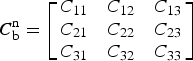 ${\bi C}_{\rm b}^{\rm n} = \left[ {\matrix{ {C_{11}} & {C_{12}} & {C_{13}} \cr {C_{21}} & {C_{22}} & {C_{23}} \cr {C_{31}} & {C_{32}} & {C_{33}} \cr}} \right]$
,
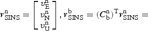 ${\bi v}_{{\rm SINS}}^{\rm n} = \left[ {\matrix{ {v_{\rm E}^{\rm n}} \cr {v_{\rm N}^{\rm n}} \cr {v_{\rm U}^{\rm n}} \cr}} \right], {\bi v}_{{\rm SINS}}^{\rm b} = ({\bi C}_{\rm b}^{\rm n} )^{\rm T} {\bi v}_{{\rm SINS}}^{\rm n}= $
 $ \left[ {\matrix{ {v_{\rm x}^{\rm b}} \cr {v_{\rm y}^{\rm b}} \cr {v_{\rm z}^{\rm b}} \cr}} \right]$
,
 ${\bi \phi} ^{\rm n} = \left[ {\matrix{ {\phi _{\rm E}} \cr {\phi _{\rm N}} \cr {\phi _{\rm U}} \cr}} \right]$
.
According to Equation (10),
 ${\bi L}$
can be presented as
 $${\bi L} = \left[ {\matrix{ {({\bi C}_{\rm b}^{\rm n} )^{\rm T}} & {{\bi M}_1} & {{\bf 0}_{3 \times 9}} & {{\bi M}_2} \cr}} \right]$$
where
 $${\bi M}_1 = \left[ {\matrix{ {C_{31} v_{\rm N}^{\rm n} - C_{21} v_{\rm U}^{\rm n}} \cr {C_{32} v_{\rm N}^{\rm n} - C_{22} v_{\rm U}^{\rm n}} \cr {C_{33} v_{\rm N}^{\rm n} - C_{23} v_{\rm U}^{\rm n}} \cr} \;\;\matrix{ {C_{11} v_{\rm U}^{\rm n} - C_{31} v_{\rm E}^{\rm n}} \cr {C_{12} v_{\rm U}^{\rm n} - C_{32} v_{\rm E}^{\rm n}} \cr {C_{13} v_{\rm U}^{\rm n} - C_{33} v_{\rm E}^{\rm n}} \cr} \;\;\matrix{ {C_{21} v_{\rm E}^{\rm n} - C_{11} v_{\rm N}^{\rm n}} \cr {C_{22} v_{\rm E}^{\rm n} - C_{12} v_{\rm N}^{\rm n}} \cr {C_{23} v_{\rm E}^{\rm n} - C_{13} v_{\rm N}^{\rm n}} \cr}} \right],\,\,{\bi M}_2 = \left[ {\matrix{ 0 & 0 & {v_{\rm y}^{\rm b}} \cr { - v_{{\rm OD}}} & 0 & 0 \cr 0 & { - v_y^{\rm b}} & 0 \cr}} \right].$$
As shown in Equation (12), the measurement matrix
 ${\bi L}$
in this paper is different from Xiao et al. (Reference Xiao, Wang, Cheng, Fu and Liu2012). The measurement coefficients of installation errors in this paper is the velocity calculated by SINS in the b frame while the one in Xiao et al. (Reference Xiao, Wang, Cheng, Fu and Liu2012) is the measurement velocity obtained by OD in the n′ frame. When an OD fault occurs, the information of the OD fault has no impact on the measurement coefficients of installation errors in this paper. Therefore, after isolating the OD's output, the navigation system can switch into the navigation mode aided by vehicle kinematic constraints (Fu et al., Reference Fu, Qin, Li and Wang2012).
The dimension of state vector in this model Equations (1) and (11) is 18, which reduces the computational efficiency of the Kalman filter. TKF is a good solution for this problem. To apply TKF, the error model of the SINS/OD integrated navigation system is translated as the following form:
 $$\left\{ \matrix{{\dot {\bi x}} = {\bi Ax} + {\bi Bb} + {\bi Gw} \hfill \cr {\bi y} = {\bi Hx} + {\bi Db} + {\bi v} \hfill} \right.$$
where
 ${\bi x} = [\matrix{ {(\delta {\bi v}_{{\rm SINS}}^{\rm n} )^{\rm T}} & {({\bi \phi} ^{\rm n} )^{\rm T}} & {(\delta {\bi p}{\rm )}^{\rm T}} \cr} ]^{\rm T} $
is the system state with nine dimensions,
 ${\bi b} = [\matrix{ {({\nabla}^{\rm b} )^{\rm T}} & {({\bi \varepsilon} ^{\rm b} )^{\rm T}} & {\matrix{ {\delta k} & {\delta \theta} & {\delta \psi} \cr}} \cr} ]^{\rm T} $
is the constant bias vector with nine dimensions,
 ${\bi w} = {\rm [}\matrix{ {w_{{\rm ax}}} & {w_{{\rm ay}}} & {w_{{\rm az}}} & {w_{{\rm gx}}} & {w_{{\rm gy}}} & {w_{{\rm gz}}} \cr} {\rm ]}^{\rm T} $
is the system process noise,
 ${\bi v}$
is the system measurement noise. The state matrix
 ${\bi A}$
is the same as
Φ
9×9 (
Φ
9×9 denotes the nine-dimensional matrix in the upper left corner of the matrix
Φ
). Matrices
 ${\bi B}$
,
 ${\bi G}$
,
 ${\bi H}$
and
 ${\bi D}$
are given as
 $${\bi B} = \left[ {\matrix{ {{\bi C}_{\rm b}^{\rm n}} & {{\bf 0}_{3 \times 3}} & {{\bf 0}_{3 \times 3}} \cr {{\bf 0}_{3 \times 3}} & {{\bi C}_{\rm b}^{\rm n}} & {{\bf 0}_{3 \times 3}} \cr {{\bf 0}_{3 \times 3}} & {{\bf 0}_{3 \times 3}} & {{\bf 0}_{3 \times 3}} \cr}} \right],\,{\bi G} = \left[ {\matrix{ {{\bi C}_{\rm b}^{\rm n}} & {{\bf 0}_{3 \times 3}} \cr {{\bf 0}_{3 \times 3}} & {{\bi C}_{\rm b}^{\rm n}} \cr {{\bf 0}_{3 \times 3}} & {{\bf 0}_{3 \times 3}} \cr}} \right],\,{\bi H} = \left[ {\matrix{ {({\bi C}_{\rm b}^{\rm n} )^{\rm T}} & {{\bi M}_1} & {{\bf 0}_{3 \times 3}} \cr}} \right],\, {\bi D} = \left[ {\matrix{ {{\bf 0}_{3 \times 6}} & {{\bi M}_2} \cr}}\right].$$
Equation (13) is transformed into the discrete-time form as
 $$\left\{ \matrix{{\bi x}_k = {\bi A}_{k,k - 1} {\bi x}_{k - 1} + {\bi B}_{k,k - 1} {\bi b} + {\bi G}_{k,k - 1} {\bi w}_{k - 1} \hfill \cr {\bi y}_k = {\bi H}_k {\bi x}_k + {\bi D}_k {\bi b} + {\bi v}_k \hfill} \right.$$
where
 ${\bi A}_{k,k - 1} $
,
 ${\bi B}_{k,k - 1} $
,
 ${\bi G}_{k,k - 1} $
,
 ${\bi H}_k $
and
 ${\bi D}_k $
are the discrete-time forms of
 ${\bi A}$
,
 ${\bi B}$
,
 ${\bi G}$
,
 ${\bi H}$
and
 ${\bi D}$
, respectively. The process noise
 ${\bi w}_k $
and the measurement noise
 ${\bi v}_k $
are zero-mean white Gaussian sequences with the following covariances:
 $E[{\bi w}_k {\bi w}_j^{\rm T} ] = {\bi Q}_k^x \delta _{kj} $
,
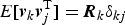 $ E[ {\bi v}_k {\bi v}_j^{\rm T} ] = {\bi R}_k \delta _{kj} $
,
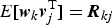 $E[{\bi w}_k {\bi v}_j^{\rm T} ] = {\bi R}_{kj}$
(
 $ {\bi Q}_k^x \gt 0$
,
 ${\bi R}_k \gt 0$
and δ
kj
is the Kronecker delta).
3. TKF ALGORITHM.
3.1. TKF Algorithm for The Linear System with Constant Bias Vector
The conventional TKF algorithm for the linear system with the constant bias vector is described by (Friedland, Reference Friedland1969; Ignagni, Reference Ignagni1981)
 $${\hat {\bi x}}_{k,k - 1} = {\tilde {\bi x}}_{k,k - 1} + {\bi U}_k {\hat {\bi b}}_{k,k - 1} $$
 $${\hat {\bi x}}_k = {\tilde {\bi x}}_k + {\bi V}_k {\hat {\bi b}}_k $$
 $${\bi P}_{k,k - 1}^x = {\tilde {\bi P}}_{k,k - 1}^x + {\bi U}_k {\bi P}_{k,k - 1}^b {\bi U}_k^{\rm T} $$
 $${\bi P}_k^x = {\tilde {\bi P}}_k^x + {\bi V}_k {\bi P}_k^b {\bi V}_k^{\rm T} $$
- BFE:
 $${\tilde {\bi x}}_{k,k - 1} = {\bi A}_{k,k - 1} {\tilde {\bi x}}_{k - 1} $$
 $${\tilde {\bi P}}_{k,k - 1}^x = {\bi A}_{k,k - 1} {\tilde {\bi P}}_{k - 1}^x {\bi A}_{k,k - 1}^{\rm T} + {\bi G}_{k,k - 1} {\bi Q}_{k - 1}^x {\bi G}_{k,k - 1}^{\rm T} $$
 $${\tilde {\bi K}}_k^x = {\tilde {\bi P}}_{k,k - 1}^x {\bi H}_k^{\rm T} [{\bi H}_k {\tilde {\bi P}}_{k,k - 1}^x {\bi H}_k^{\rm T} + {\bi R}_k ]^{ - 1} $$
 $${\tilde {\bi x}}_k = {\tilde {\bi x}}_{k,k - 1} + {\tilde {\bi K}}_k^x [{\bi y}_k - {\bi H}_k {\tilde {\bi x}}_{k,k - 1} ]$$
 $${\tilde {\bi P}}_k^x = [{\bi I} - {\tilde {\bi K}}_k^x {\bi H}_k ]{\tilde {\bi P}}_{k,k - 1}^x $$
- BE:
 $${\hat {\bi b}}_{k,k - 1} = {\hat {\bi b}}_{k - 1} $$
 $${\bi P}_{k,k - 1}^b = {\bi P}_{k - 1}^b $$
 $${\bi K}_k^b = {\bi P}_{k,k - 1}^b {\bi S}_k^{\rm T} [{\bi H}_k {\tilde {\bi P}}_{k,k - 1}^x {\bi H}_k^{\rm T} + {\bi S}_k {\bi P}_{k,k - 1}^b {\bi S}_k^{\rm T} + {\bi R}_k ]^{ - 1} $$
 $${\hat {\bi b}}_k = {\hat {\bi b}}_{k,k - 1} + {\bi K}_k^b [{\bi r}_k^x - {\bi S}_k {\hat {\bi b}}_{k,k - 1} ]$$
 $${\bi P}_k^b = [{\bi I} - {\bi K}_k^b {\bi S}_k ]{\bi P}_{k,k - 1}^b $$
with the coupling equations
 $${\bi U}_k = {\bi A}_{k,k - 1} {\bi V}_{k - 1} + {\bi B}_{k,k - 1} $$
 $${\bi V}_k = {\bi U}_k - {\tilde {\bi K}}_k^x {\bi S}_k $$
 $${\bi S}_k = {\bi H}_k {\bi U}_k + {\bi D}_k $$
 $${\bi r}_k^x = {\bi y}_k - {\bi H}_k {\tilde {\bi x}}_{k,k - 1} $$
3.2. Innovations in TKF
Lemma 1. The innovation
 ${\bi r}_k^x = ({\bi y}_k - {\bi H}_k {\tilde {\bi x}}_{k,k - 1} )$
in BFE is not zero-mean.
Proof. The two-stage Kalman filter is optimal in the sense that it is equivalent to the GKF. Thus, the estimates
 ${\hat {\bi x}}_k $
and
 ${\hat {\bi b}}_k $
are the unbiased estimates of the states
 ${\bi x}_k $
and
 ${\bi b}$
, i.e.
 $E[{\hat {\bi x}}_k ] = E[{\bi x}_k ]$
,
 $E[{\hat {\bi b}}_k ] = E[{\bi b}_k ] = {\bi b}$
.
Using Equation (14), the innovation can be written as
 $$\eqalign{{\bi r}_k^x & = {\bi y}_k - {\bi H}_k {\tilde {\bi x}}_{k,k - 1} \quad \cr & = {\bi H}_k ({\bi A}_{k,k - 1} {\bi x}_{k - 1} + {\bi B}_{k,k - 1} {\bi b} + {\bi G}_{k,k - 1} {\bi w}_{k - 1} ) \quad \cr & \quad + {\bi D}_k {\bi b} + {\bi v}_k - {\bi H}_k {\bi A}_{k,k - 1} {\tilde {\bi x}}_{k - 1} }$$
Substituting Equation (16) into Equation (33), the above becomes
 $$\eqalign{{\bi r}_k^x & = {\bi H}_k ({\bi A}_{k,k - 1} {\bi x}_{k - 1} + {\bi B}_{k,k - 1} {\bi b} + {\bi G}_{k,k - 1} {\bi w}_{k - 1} ) +{\bi D}_k {\bi b} + {\bi v}_k - {\bi H}_k {\bi A}_{k,k - 1} ({\hat {\bi x}}_{k - 1} - {\bi V}_{k - 1} {\hat {\bi b}}_{k - 1} ) \quad \cr & = {\bi H}_k {\bi A}_{k,k - 1} ({\bi x}_{k - 1} - {\hat {\bi x}}_{k - 1} ) + {\bi H}_k {\bi G}_{k,k - 1} {\bi w}_{k - 1} + {\bi v}_k + ({\bi H}_k {\bi B}_{k,k - 1} + {\bi D}_k ){\bi b}\cr & \qquad +{\bi H}_k {\bi A}_{k,k - 1} {\bi V}_{k - 1} {\hat {\bi b}}_{k - 1}}$$
Then, the expected value of
 ${\bi r}_k^x $
is
 $$\eqalign{E[{\bi r}_k^x ] & = E[{\bi H}_k {\bi A}_{k,k - 1} ({\bi x}_{k - 1} - {\hat {\bi x}}_{k - 1} ) + {\bi H}_k {\bi G}_{k,k - 1} {\bi w}_{k - 1} + {\bi v}_k \quad \cr &\quad + ({\bi H}_k {\bi B}_{k,k - 1} + {\bi D}_k ){\bi b + H}_k {\bi A}_{k,k - 1} {\bi V}_{k - 1} {\hat {\bi b}}_{k - 1} ] \quad \cr & = {\bi H}_k {\bi A}_{k,k - 1} (E[{\bi x}_{k - 1} ] - E[{\hat {\bi x}}_{k - 1} ]) + {\bi H}_k {\bi G}_{k,k - 1} E[{\bi w}_{k - 1} ] + E[{\bi v}_k ] \cr &\quad + ({\bi H}_k {\bi B}_{k,k - 1} + {\bi D}_k ){\bi b} + {\bi H}_k {\bi A}_{k,k - 1} {\bi V}_{k - 1} E[{\hat {\bi b}}_{k - 1} ] \quad \cr & = [{\bi H}_k ({\bi B}_{k,k - 1} + {\bi A}_{k,k - 1} {\bi V}_{k - 1} ) + {\bi D}_k ]{\bi b}} $$
By utilising Equation (29) and Equation (31), the above becomes
 $$E[{\bi r}_k^x ] = {\bi S}_k {\bi b}$$
In general, since
 ${\bi b}$
is a vector with no zero components and
 ${\bi S}_k $
is a nonzero matrix, then
 $E[{\bi r}_k^x ] \ne {\bf 0}$
. Thus, the innovation
 ${\bi r}_k^x = ({\bi y}_k - {\bi H}_k {\tilde {\bi x}}_{k,k - 1} )$
in BFE is not zero-mean.
From Lemma 1, it can be concluded that using the innovation
 ${\bi r}_k^x = ({\bi y}_k - {\bi H}_k {\tilde {\bi x}}_{k,k - 1} )$
as zero-mean sequence in ATKF such as Kim et al. (Reference Kim, Lee and Park2006; Reference Kim, Lee and Park2009) is not correct.
As described in Ignagni (Reference Ignagni1981), if BFE has perfect knowledge of
 ${\bi b}$
, the covariance matrix of
 $({\bi r}_k^x - {\bi S}_k {\bi b})$
is
 $$E[({\bi r}_k^x - {\bi S}_k {\bi b})({\bi r}_k^x - {\bi S}_k {\bi b})^{\rm T} ] = {\bi H}_k {\tilde {\bi P}}_{k,k - 1}^x {\bi H}_k^{\rm T} + {\bi R}_k $$
In fact, the perfect knowledge of
 ${\bi b}$
cannot be obtained. Only the estimate
 ${\hat {\bi b}}_{k,k - 1} $
of
 ${\bi b}$
by BE can be obtained. That is to say, the estimator cannot obtain the white noise sequence
 $({\bi r}_k^x - {\bi S}_k {\bi b})$
with the covariance matrix
 $({\bi H}_k {\tilde {\bi P}}_{k,k - 1}^x {\bi H}_k^{\rm T} + {\bi R}_k )$
, but only obtains the sequence
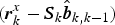 $({\bi r}_k^x - {\bi S}_k {\hat {\bi b}}_{k,k - 1} )$
which is the same as the innovation in BE.
Lemma 2. The innovation
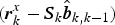 $({\bi r}_k^x - {\bi S}_k {\hat {\bi b}}_{k,k - 1} )$
in BE is identical with the innovation in GKF.
Proof. Treating
 ${\bi x}_k $
and
 ${\bi b}$
as the augmented system state, the GKF for the linear system Equation (14) is described by (Ignagni, Reference Ignagni1981)
 $${\hat {\bi z}}_{k,k - 1} = {\bi \phi} _{k,k - 1} {\hat {\bi z}}_{k - 1} $$
 $${\bi P}_{k,k - 1} = {\bi \phi} _{k,k - 1} {\bi P}_{k - 1} {\bi \phi} _{k,k - 1}^{\rm T} + {\bi G^{\prime}}_{k,k - 1} {\bi Q}_{k - 1} ({\bi G^{\prime}}_{k,k - 1} )^{\rm T} $$
 $${\bi K}_k = {\bi P}_{k,k - 1} {\bi L}_k^{\rm T} [{\bi L}_k {\bi P}_{k,k - 1} {\bi L}_k^{\rm T} + {\bi R}_k ]^{ - 1} $$
 $${\hat {\bi z}}_k = {\hat {\bi z}}_{k,k - 1} + {\bi K}_k [{\bi y}_k - {\bi L}_k {\hat {\bi z}}_{k,k - 1} ]$$
 $${\bi P}_k = [{\bi I} - {\bi K}_k {\bi L}_k ]{\bi P}_{k,k - 1} $$
where
 ${\hat {\bi z}}_k $
is the estimate of
 ${\bi z}_k $
,
 ${\bi z}_k = [\matrix{ {{\bi x}_k^{\rm T}} & {{\bi b}^{\rm T}} \cr} ]^{\rm T} $
,
 ${\bi L}_k = [\matrix{ {{\bi H}_k} & {{\bi D}_k} \cr} ], {\bi \phi} _{k,k - 1} =$
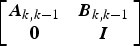 $ \left[ {\matrix{ {{\bi A}_{k,k - 1}} & {{\bi B}_{k,k - 1}} \cr {\bf 0} & {\bi I} \cr}} \right]$
,
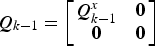 ${\bi Q}_{k - 1} = \left[ {\matrix{ {{\bi Q}_{k - 1}^x} & {\bf 0} \cr {\bf 0} & {\bf 0} \cr}} \right]$
,
 ${\bi P}_{k,k - 1} = \left[ {\matrix{ {{\bi P}_{k,k - 1}^x} & {{\bi P}_{k,k - 1}^{xb}} \cr {({\bi P}_{k,k - 1}^{xb} )^{\rm T}} & {{\bi P}_{k,k - 1}^b} \cr}} \right],{\bi G^{\prime}}_{k,k - 1} = $
 $\left[ {\matrix{ {{\bi G}_{k,k - 1}} \cr {\bf 0} \cr}} \right]$
and
 ${\bi P}_{k,k - 1}^{xb} = {\bi U}_k {\bi P}_{k,k - 1}^b $
.
The innovation in GKF is
 $({\bi y}_k - {\bi L}_k {\hat {\bi z}}_{k,k - 1} )$
with the covariance matrix
 $({\bi L}_k {\bi P}_{k,k - 1} {\bi L}_k^{\rm T} + {\bi R}_k )$
.
Using Equations (15), (31) and (32), the innovation in BE can be rewritten as
 $$\eqalign{{\bi r}_k^x - {\bi S}_k {\hat {\bi b}}_{k,k - 1} & = {\bi y}_k - {\bi H}_k {\tilde {\bi x}}_{k,k - 1} - {\bi S}_k {\hat {\bi b}}_{k,k - 1} \quad \cr & = {\bi y}_k - {\bi H}_k [{\hat {\bi x}}_{k,k - 1} - {\bi U}_k {\hat {\bi b}}_{k,k - 1} ] - [{\bi H}_k {\bi U}_k + {\bi D}_k ]{\hat {\bi b}}_{k,k - 1} \quad \cr & = {\bi y}_k - {\bi H}_k {\hat {\bi x}}_{k,k - 1} - {\bi D}_k {\hat {\bi b}}_{k,k - 1} \quad \cr & = {\bi y}_k - {\bi L}_k {\hat {\bi z}}_{k,k - 1}} $$
The covariance matrix of the innovation in BE is
 $$\eqalign{& {\bi H}_k {\tilde {\bi P}}_{k,k - 1}^x {\bi H}_k^{\rm T} + {\bi S}_k {\bi P}_{k,k - 1}^b {\bi S}_k^{\rm T} + {\bi R}_k \cr & = {\bi H}_k [{\bi P}_{k,k - 1}^x - {\bi U}_k {\bi P}_{k,k - 1}^b {\bi U}_k^{\rm T} ]{\bi H}_k^{\rm T} + [{\bi H}_k {\bi U}_k + {\bi D}_k ]{\bi P}_{k,k - 1}^b [{\bi H}_k {\bi U}_k + {\bi D}_k ]^{\rm T} + {\bi R}_k \cr & = {\bi H}_k {\bi P}_{k,k - 1}^x {\bi H}_k^{\rm T} + {\bi H}_k {\bi U}_k {\bi P}_{k,k - 1}^b {\bi D}_k^{\rm T} + {\bi D}_k {\bi P}_{k,k - 1}^b [{\bi H}_k {\bi U}_k ]^{\rm T} + {\bi D}_k {\bi P}_{k,k - 1}^b {\bi D}_k^{\rm T} + {\bi R}_k \cr & = [\matrix{ {{\bi H}_k} & {{\bi D}_k} \cr} ]\left[ {\matrix{ {{\bi P}_{k,k - 1}^x} & {{\bi U}_k {\bi P}_{k,k - 1}^b} \cr {({\bi U}_k {\bi P}_{k,k - 1}^b )^{\rm T}} & {{\bi P}_{k,k - 1}^b} \cr}} \right][\matrix{ {{\bi H}_k} & {{\bi D}_k} \cr} ]^{\rm T} + {\bi R}_k \cr & = [\matrix{ {{\bi H}_k} & {{\bi D}_k} \cr} ]\left[ {\matrix{ {{\bi P}_{k,k - 1}^x} & {{\bi P}_{k,k - 1}^{xb}} \cr {({\bi P}_{k,k - 1}^{xb} )^{\rm T}} & {{\bi P}_{k,k - 1}^b} \cr}} \right][\matrix{ {{\bi H}_k} & {{\bi D}_k} \cr} ]^{\rm T} + {\bi R}_k \cr & = {\bi L}_k {\bi P}_{k,k - 1} {\bi L}_k^{\rm T} + {\bi R}_k} $$
Therefore, the innovation
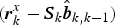 $({\bi r}_k^x - {\bi S}_k {\hat {\bi b}}_{k,k - 1} )$
in BE is identical to the innovation in GKF.
4. ATKF ALGORITHM
When developing the AKF algorithm, we employ an important property of the optimal filter, that is, the innovation in this filter is a white noise sequence with zero-mean when the filter is optimal (Xia et al., Reference Xia, Rao, Ying and Shen1994; Mohamed and Schwarz, Reference Mohamed and Schwarz1999; Hide et al., Reference Hide, Moore and Smith2003; Geng and Wang, Reference Geng and Wang2008; Shi et al., Reference Shi, Miao and Ni2010; Gao et al., Reference Gao, Miao and Ni2011). Through Lemma 1 and 2, it can be concluded that only the innovation
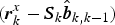 $({\bi r}_k^x - {\bi S}_k {\hat {\bi b}}_{k,k - 1} )$
in BE can be used in an ATKF algorithm. Lemma 2 shows the innovation
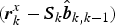 $({\bi r}_k^x - {\bi S}_k {\hat {\bi b}}_{k,k - 1} )$
in BE is the same as the innovation in Zhao et al. (Reference Zhao, Miao and Shen2014). Thus, the method of detecting an OD fault in Zhao et al. (Reference Zhao, Miao and Shen2014) is employed to form the multiple adaptive factors scheme in ATKF.
4.1. Fault diagnosis
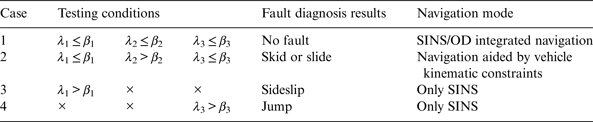
If a vehicle skids or slides, OD outputs false information. If a vehicle sideslips or jumps, the condition of vehicle kinematic constraints is broken. Thus, the system must have the ability of fault diagnosis.
Suppose that
 ${\bi r}_k^b = {\bi r}_k^x - {\bi S}_k {\hat {\bi b}}_{k,k - 1} $
and
 ${\bi M}_k = {\bi H}_k {\tilde {\bi P}}_{k,k - 1}^x {\bi H}_k^{\rm T} + {\bi S}_k {\bi P}_{k,k - 1}^b {\bi S}_k^{\rm T} + {\bi R}_k $
. As indicated by Lemma 2,
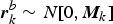 ${\bi r}_k^b \sim N[0,{\bi M}_k ]$
and
 ${\bi r}_k^b = {\bi y}_k - {\bi L}_k {\hat {\bi z}}_{k,k - 1} $
when TKF is optimal. When the vehicle skids, slides, sideslips or jumps, the expectation of
 ${\bi r}_k^b $
would become non-zero and/or its covariance larger than
 ${\bi M}_k $
. A simple and effective testing approach for this case is the chi-square test (Shi et al., Reference Shi, Miao and Ni2010). From the fact that the normalised sequence
 $$\lambda _i = \displaystyle{{[{\bi r}_k^b (i)]^2} \over {{\bi M}_k (i,i)}} \sim \chi ^2 (1)$$
is chi-square distributed with one degree of freedom, where
 ${\bi r}_k^b (i)$
and
 ${\bi M}_k (i,i)$
are, respectively, the ith component of
 ${\bi r}_k^b $
and the ith diagonal component of
 ${\bi M}_k $
.
Zhao et al. (Reference Zhao, Miao and Shen2014) indicates that the innovation consists of
 ${\bi y}_k $
and
 ${\bi L}_k {\hat {\bi z}}_{k,k - 1} $
. The fault information affects the innovation only by
 ${\bi y}_k $
and
 ${\bi L}_k $
. Since the measurement vector
 ${\bi y}_k $
can be described as
 ${\bi y}_k = {\hat {\bi v}}_{{\rm INS}}^{\rm b} - {\hat {\bi v}}_{{\rm OD}}^{\rm m} = [\matrix{ {\hat v_{\rm x}^{\rm b}} & {\hat v_{\rm y}^{\rm b} - \hat v_{{\rm OD}}} & {\hat v_{\rm z}^{\rm b}} \cr} ]^{\rm T} $
, it can be determined that the OD's fault information only affects the measurement information
 ${\bi y}_k (2)$
. Otherwise,
 ${\bi y}_k (1)$
is affected when the vehicle sideslips and
 ${\bi y}_k (3)$
is affected when the vehicle jumps, where
 ${\bi y}_k (i)$
is the ith component of
 ${\bi y}_k $
(i = 1, 2, 3). As shown in Equation (12), the OD fault information affects the measurement matrix
 ${\bi L}_k $
, and only
 ${\bi r}_k^b (2)$
is affected by
 ${\bi L}_k {\hat {\bi z}}_{k,k - 1} $
. From the above discussion, the fault criteria are obtained as Table 1.
Fault criterions.

Note: β i (i = 1, 2, 3) is the threshold obtained from the chi-square distribution table with the required rates of the missing and false detection, × denotes no need to test the condition.
4.2. Adaptive Fading Algorithm
As the same as Kim et al. (Reference Kim, Lee and Park2006; Reference Kim, Lee and Park2009), the adaptive factors are inserted into the prior error covariance equations as the following forms
 $${\tilde {\bi P}}_{k,k - 1}^x = \lambda _k^x [{\bi A}_{k,k - 1} {\tilde {\bi P}}_{k - 1}^x {\bi A}_{k,k - 1}^{\rm T} + {\bi G}_{k,k - 1} {\bi Q}_{k - 1}^x {\bi G}_{k,k - 1}^{\rm T} ]$$
 $${\bi P}_{k,k - 1}^b = \lambda _k^b {\bi P}_{k - 1}^b $$
In AKF algorithms (Xia et al., Reference Xia, Rao, Ying and Shen1994), if an adaptive factor can be chosen so that
 $${\bi P}_{k,k - 1} {\bi H}_k^{\rm T} - {\bi K}_k {\bi C}_k = 0$$
then the filter is optimal. The optimal condition Equation (42) is equivalent to
 $${\bi H}_k {\bi P}_{k,k - 1} {\bi H}_k^{\rm T} + {\bi R}_k = {\bi C}_k $$
where
 ${\bi C}_k $
in Equations (42) and (43) is the real covariance matrix of innovation which is computed from measured data.
By the optimal condition Equation (43) and Lemma 2, the optimal condition in ATKF algorithm is
 $${\bi H}_k {\tilde {\bi P}}_{k,k - 1}^x {\bi H}_k^{\rm T} + {\bi S}_k {\bi P}_{k,k - 1}^b {\bi S}_k^{\rm T} + {\bi R}_k = {\bi C}_k^b $$
where
 ${\bi C}_k^b $
is the real covariance matrix of innovation in BE which is computed from measured data.
From the discussion in Section 4.1, it can be determined that the changes of the OD scale factor error and the process noise also affect the innovation. The change of the OD scale factor error would lead to a change in OD's output, thus it can affect
 ${\bi r}_k^b (2)$
but has no impact on the other components of the innovation. When the process noises change, one component at least would be affected. Then, the adaptive rules are obtained as Table 2.
Adaptive rules.

Note: ε i (i = 1, 2, 3) is the threshold obtained from the chi-square distribution table with the chosen false alarm probability ξ i .
As shown in Tables 1 and 2, the fault criteria seem to conflict with the adaptive rules. In general, the innovation is more seriously affected by the vehicle skid, slide, sideslip and jump than by the changes of the OD scale factor error and the process noise, and λ i (i = 1, 2, 3) calculated by the chi-square test in the fault criterions is much bigger than the one in the adaptive rules. So the threshold β i (i = 1, 2, 3) is much higher than ε i . Therefore in the execution process of the algorithm proposed in this paper, the fault diagnosis must be implemented at first, and, only when the result of fault diagnosis is no fault, the adaptive algorithm can be implemented. From the discussion, it can be seen that there is no conflict between the fault criteria and the adaptive rules.
In case 1,
 $\lambda _k^x = \lambda _k^b = 1$
implies that ATKF functions in the same way as the normal TKF and provides the optimal estimation.
In case 2, when the OD scale factor error changes,
 $\lambda _k^x = 1$
and
 $\lambda _k^b $
needs to be computed. Substitution of Equations (40) and (41) into Equation (44) results in the following
 $$\lambda _k^b {\bi S}_k {\bi P}_{k - 1}^b {\bi S}_k^{\rm T} = {\bi C}_k^b - {\bi R}_k - {\bi H}_k {\tilde {\bi P}}_{k,k - 1}^x {\bi H}_k^{\rm T} $$
Take trace in both sides of Equation (45), then
 $\lambda _k^b $
can be obtained as
 $$\lambda _k^b = {{{\rm trace}[{\bi C}_k^b - {\bi R}_k - {\bi H}_k {\tilde {\bi P}}_{k,k - 1}^x {\bi H}_k^{\rm T} ]} / {{\rm trace}[{\bi S}_k {\bi P}_{k - 1}^b {\bi S}_k^{\rm T} ]}}$$
and
 $\lambda _k^b \ge 1$
.
In case 3, when
 ${\bi Q}_k^x $
changes (at the same time, δk may change),
 $\lambda _k^x = \lambda _k^b $
. Substitute Equations (40) and (41) into Equation (44), then Equation (44) can be expressed as
 $$\lambda _k^x {\bi H}_k [{\bi A}_{k,k - 1} {\tilde {\bi P}}_{k - 1}^x {\bi A}_{k,k - 1}^{\rm T} + {\bi G}_{k,k - 1} {\bi Q}_{k - 1}^x {\bi G}_{k,k - 1}^{\rm T} ]{\bi H}_k^{\rm T} + \lambda _k^b {\bi S}_k {\bi P}_{k - 1}^b {\bi S}_k^{\rm T} = {\bi C}_k^b - {\bi R}_k $$
Since
 $\lambda _k^x = \lambda _k^b $
, Equation (47) can be written as
 $$\lambda _k^x \left[ {{\bi H}_k [{\bi A}_{k,k - 1} {\tilde {\bi P}}_{k - 1}^x {\bi A}_{k,k - 1}^{\rm T} + {\bi G}_{k,k - 1} {\bi Q}_{k - 1}^x {\bi G}_{k,k - 1}^{\rm T} ]{\bi H}_k^{\rm T} + {\bi S}_k {\bi P}_{k - 1}^b {\bi S}_k^{\rm T}} \right] = {\bi C}_k^b - {\bi R}_k $$
Take trace in both sides of Equation (48), then
 $\lambda _k^x $
and
 $\lambda _k^b $
can be obtained as
 $$\lambda _k^x = \lambda _k^b = {{{\rm trace}\left[ {{\bi C}_k^b - {\bi R}_k} \right]} / {{\rm trace}\left[ {{\bi H}_k [{\bi A}_{k,k - 1} {\tilde {\bi P}}_{k - 1}^x {\bi A}_{k,k - 1}^{\rm T} + {\bi G}_{k,k - 1} {\bi Q}_{k - 1}^x {\bi G}_{k,k - 1}^{\rm T} ]{\bi H}_k^{\rm T} + {\bi S}_k {\bi P}_{k - 1}^b {\bi S}_k^{\rm T}} \right]}}$$
and
 $\lambda _k^x = \lambda _k^b \ge 1$
.
4.3. Algorithm of Computing C k b
In the process of computing the adaptive factors
 $\lambda _k^x $
and
 $\lambda _k^b $
,
 ${\bi C}_k^b $
is employed as the real covariance matrix of innovation in BE which is computed from measured data. Only when
 ${\bi C}_k^b $
accurately indicates the changes of the innovation covariance, the adaptive factors
 $\lambda _k^x $
and
 $\lambda _k^b $
can be computed optimally. Through improving the method presented in Xia et al. (Reference Xia, Rao, Ying and Shen1994), a novel algorithm for computing
 ${\bi C}_k^b $
is proposed as:
 $${\bi \alpha} _k (i) = {{{\bi \alpha} _{k - 1} (i)} / {\rho _i}} + [{\bi r}_k^b (i)]^2 $$
 $${\bi \gamma} _k (i) = {{{\bi \gamma} _{k - 1} (i)} / {\rho _i}} + 1$$
 $${\bi C}_k^b (i,i) = {{{\bi \alpha} _k (i)} / {{\bi \gamma} _k (i)}}$$
where
 ${\bi r}_k^b (i)$
is the ith element of the innovation
 ${\bi r}_k^b $
, the adaptive factors ρ
1 = ρ
2 = ρ
3 = ρ in case 1 (ρ is slightly greater than 1, generally ρ = 1·001), ρ
1 = ρ
3 = ρ and
 $\rho _2 = (\xi )^{{\rm INT}(\lambda _2 )} $
in case 2 (
 ${\rm INT}(*)$
denotes the rounding function, ξ is slightly greater than 1, generally ξ = 1·01),
 $\rho _i = (\xi )^{{\rm INT}(\lambda _i )} $
in case 3 (i = 1, 2, 3), λ
i
(i = 1, 2, 3) is defined in Section 4.1. The initial conditions are
 ${\bi \alpha} _0 (i) = 0$
and
 ${\bi \gamma} _0 (i) = 0$
(i = 1, 2, 3).
The method of computing
 ${\bi C}_k^b $
in Xia et al. (Reference Xia, Rao, Ying and Shen1994) used the adaptive factor calculated in the last step. The adaptive factor may be far greater than 1 because of the influence of the random noise. Therefore, the value of the innovation covariance computed by this method may fluctuate when the innovation remains unchanged. This fluctuation incorrectly indicates the change of innovation. The algorithm for computing
 ${\bi C}_k^b $
in this paper can not only ensure the stability of
 ${\bi C}_k^b $
in the false alarm case of the chi-square test, but also ensure the ability to track the change of innovation, which guarantees the accurate calculation of adaptive factors.
5. SIMULATION RESULTS AND ANALYSIS
Simulation conditions are set as follows: the constant drift and random noise of each gyro are 0·02o/h and 0·02o/h(1σ) respectively; the constant bias and random noise of each accelerometer are 1 × 10⁻⁴ g and 1 × 10⁻⁴ g(1σ) respectively; the OD scale factor error is 0·002; each installation error angles is 0·5°; after the initial alignment, the horizontal accuracy is 1′, and the azimuth accuracy is 10′; the initial latitude error, longitude error and height error are 10 m respectively.
The simulation time is 1 h. At first, the vehicle remains static for 100 s, and then begins to move. The trajectory is shown as Figure 1, and the total distance is about 49 km. The vehicle manoeuvres mainly include the course turn, acceleration and deceleration, where the maximum acceleration is 3 m/s2 and the maximum speed is 20 m/s.
Vehicle trajectory.

5.1. Algorithm performance verification
To verify the performance of ATKF for the SINS/OD integrated navigation system, we set the changes of the OD scale factor error and the process noise as Table 3.
Changes of states.

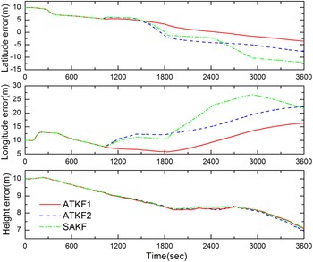
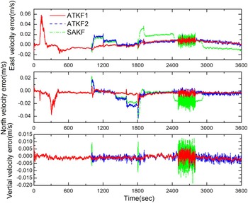
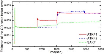
Suppose that the ATKF proposed in this paper is denoted as ATKF1, the ATKF formed by the adaptive algorithm in Kim et al. (Reference Kim, Lee and Park2006; Reference Kim, Lee and Park2009) is denoted as ATKF2 and the single adaptive factor Kalman filter presented in Xia et al. (Reference Xia, Rao, Ying and Shen1994) is denoted as SAKF. Comparing these three filters, the results are shown in Figures 2, 3 and 4.
Position errors.

Velocity errors.

Estimate of the OD scale factor error.

Figures 2, 3 and 4 show respectively the position errors, velocity errors and estimate of the OD scale factor error after the corrections to the output of the SINS/OD integrated navigation system by the three filters. As shown in Figures 2 and 3, for the SINS/OD integrated navigation system, the position errors and velocity errors using ATKF1 are significantly smaller than using ATKF2 and SAKF. In Figure 2, there is significant difference in the latitude and longitude direction between the three methods, but the difference is small in the height direction. That is because the vehicle moves only in the horizontal plane but not in the height direction.
In Figure 4, when the OD scale factor error first changes, ATKF2 cannot identify this change, but ATKF1 is able to track the change of the OD scale factor error well. As mentioned in Section 1, ATKF2 employs that the innovation in BFE is a white noise sequence with zero-mean, but Lemma 1 indicates the mean of the innovation in BFE is
 ${\bi S}_k {\bi b}$
. Thus, in the ATKF2 algorithm, the probability that the adaptive factor in BFE incorrectly functions would be greatly increased. From the optimal condition Equation (44), that would damage the optimal condition of filtering and degrade the performance of filtering, which causes the position and velocity errors to increase. At the same time, the case that ATKF2 cannot track the first change of the OD scale factor error, further exacerbates the performance degradation of filtering; when ATKF2 estimates the second change of the OD scale factor error, the performance of filtering is improved (seen in Figure 3). When the OD scale factor error changes for the first time, the incorrect function of the adaptive factor in BFE interferes with the calculation of the adaptive factor in BE, which causes ATKF2 to fail to track the change of the OD scale factor error; when the OD scale factor error changes for the second time, since the error accumulates to a certain extent, the adaptive algorithm in BE functions in the right way, then the OD scale factor error is estimated, but its estimation precision is still lower than ATKF1.
As shown in Figures 2 and 3, the position errors and velocity errors using SAKF are the biggest in the three filters. At the same time, Figure 4 shows that the estimation accuracy of the OD scale factor error using SAKF is the lowest. Since SAKF has only one adaptive factor, it cannot distinguish the change of the OD scale factor error from the change of the process noise. Therefore, the estimation error of δk is much bigger than the other two filters, which is the main reason that the position errors and velocity errors using SAKF are the biggest.
5.2. Algorithm performance verification with fault
To verify the performance of ATKF1 when the fault occurs, we increase the fault conditions as Table 4 on the basis of the vehicle motion states in Section 5.1.
Fault conditions.

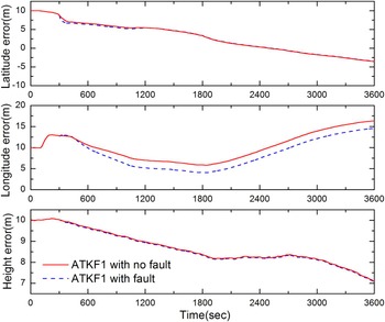
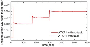
To verify the performance of ATKF1 when the fault occurs, the simulation results with fault and with no fault are both presented. As shown in Figure 5, the differences between the two results with regard to the position errors are very little. The position accuracy with fault is basically equivalent to that with no fault. Figure 6 shows that the estimation accuracy of the OD scale factor error with fault is almost as same as that with no fault. When the fault occurs, ATKF1 still has the ability to track the changes of the OD scale factor error. It can be concluded that ATKF1 can handle the problems of fault diagnosis and adaptive adjustment simultaneously.
Position errors.

Estimate of the OD scale factor error.

6. REAL EXPERIMENT RESULTS AND ANALYSIS
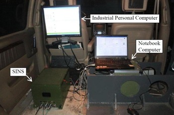
To further verify the performance of the proposed algorithm, a real experiment is carried out. The experimental equipment is shown in Figure 7. The differential GPS receiver is fitted on the roof of the experimental vehicle, and the OD is installed on the driving wheels of the experimental vehicle. By error compensation, the statistical characteristics of inertial devices in SINS are as follows: the constant drift of each fibre optic gyro is about 0·1o/h, and the random noise is about 0·2o/h(1σ); the constant bias of each accelerometer is about 5 × 10⁻⁵ g, and the random noise is about 1 × 10⁻⁴ g(1σ). The data acquisition periods of the inertial measurement unit (IMU) and the OD are 5 ms and 20 ms respectively, and the filtering period is set to 20 ms.
Experimental equipment.

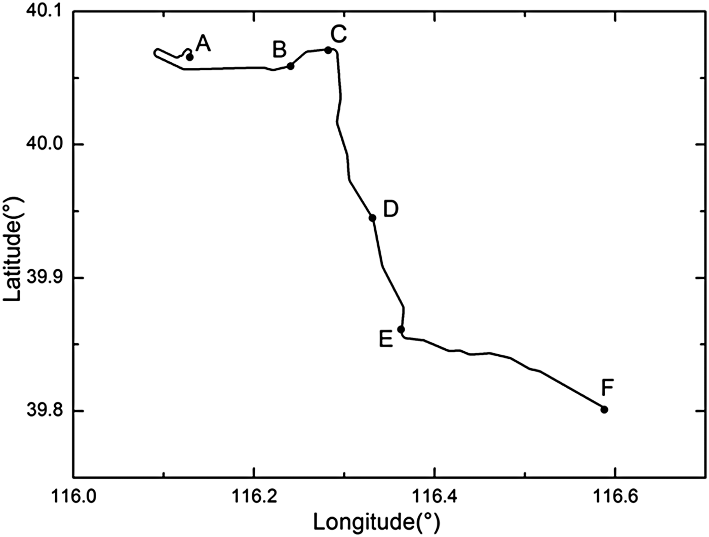
All of the experimental data is stored in the external computers. In order to prevent data loss, a notebook computer and an industrial personal computer are both used to store the experimental data. Then, the method of offline calculation is adopted to validate the performance of the proposed algorithm. The differential GPS positioning accuracy is about 1 m, and its positioning results are used as a positioning reference to evaluate the positioning accuracy of the SINS/OD integrated navigation system. Figure 8 shows a trajectory of the experimental vehicle, which only shows the changes in the directions of latitude and longitude (the height variation throughout the process of experiment is less than 5 m). The experimental vehicle starts from point A and ends at point F. The whole experiment lasts 3,600 s, and the total distance is about 55 km.
Experimental vehicle trajectory.

As we were limited by the conditions of this experimental road in Beijing, it is difficult to achieve the OD scale factor error changes in the experimental process, and the faults of vehicle skids, slides, sideslips and jumps are also difficult to achieve. In practice, when the vehicle skids, the OD output speed is generally much larger than the true value of vehicle speed; while when the vehicle slides, the OD output speed is less than the real speed of vehicle, and in extreme instances the OD output speed is zero. To verify the effectiveness of the proposed algorithm, while the offline data is kept close to the actual situation as much as possible, the offline data is processed in two ways: first, the OD output value between 1,200 s – 2,500 s is multiplied by a fixed coefficient of 1·0005 to simulate the OD scale factor error changes, and the corresponding traveling track is from point C to point E in Figure 8; second, the OD output value between 1,000 s – 1,010 s plus a fixed value of 10 m/s simulates the vehicle skid, while the OD output value between 2,000 s – 2,010 s is set to 0, to simulate the vehicle slide, which respectively correspond to point B and point D in Figure 8 (as the travelling distances of the experimental vehicle are too short in the time of 10 s, the points B and D are used to represent the moving trajectories of vehicle skid and slide respectively).
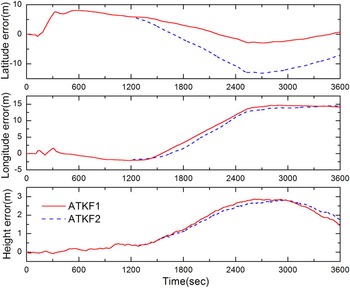
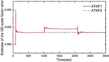
In the actual experiment, two algorithms of ATKF1 and ATKF2 are compared. Figure 9 shows the positioning errors of the integrated navigation system using ATKF1 and ATKF2 respectively. The results show that the positioning accuracy using ATKF1 is much higher than using ATKF2. As shown in Figure 10, the initial estimates of the OD scale factor error by ATKF1 and ATKF2 are both about 0·001386; After the OD scale factor error changed, the estimate of the OD scale factor error by ATKF1 is about 0·001854 while the estimate by ATKF2 is still about 0·001386. According to that, the OD output value between 1,200 s – 2,500s is multiplied by a fixed coefficient of 1·0005, and the initial estimates of the OD scale factor error is about 0·001386, we can calculate that the changed OD scale factor error is about 0·001887 (the calculation method is:1·001386 × 1·0005 − 1 ≈ 0·001887). Thus, the estimate of the changed OD scale factor error is basically consistent with the actual value. From the above discussion, the conclusion can be reached that ATKF1 has good performance in tracking the change of the OD scale factor error, while ATKF2 cannot distinguish the change of the OD scale factor error, which is the main reason that the positioning accuracy using ATKF1 is better than using ATKF2.
Position errors.

Estimate of the OD scale factor error.

It should be noted that in the process of the experiment, the same fault diagnosis algorithm is used in both ATKF1 and ATKF2. That can minimise the effects of vehicle skids and slides on the performance of the two algorithms. Therefore, our conclusion about the two algorithms’ performance comparison is objective and reliable.
7. CONCLUSION
This paper first analyses the problems of ATKF in Kim et al. (Reference Kim, Lee and Park2006; Reference Kim, Lee and Park2009) and proves that only the innovation in BE can be used in the ATKF algorithm. On this basis, a novel multiple adaptive factors ATKF algorithm is presented through utilising the method of detecting an OD fault in Zhao et al. (Reference Zhao, Miao and Shen2014), which is used to solve the problem that the changes of the OD scale factor error and the process noise degrades the filtering performance. This algorithm has the same advantages as TKF; for example, it mitigates the computational difficulties associated with large matrices and it is suitable for parallel computing hardware design. The performance of the ATKF proposed in this paper has been verified by simulations and actual experiments.
The algorithm derived in this paper is based on unknown constant biases. For situations where the biases are randomly varying, the corresponding algorithm requires further research.
FINANCIAL SUPPORT
This work was supported by National Natural Science Foundation of China (grant number 61153002).