


When politicians formulate policies, they weigh many factors. Does the policy help achieve political and ideological goals or advance moral values? Is the policy likely to be successful and cost efficient? To answer these questions, policy makers may rely on information from within their polities, as well as from without. Internally, they may learn about the preferences of the public, the goals of interest groups and other politicians, and the effects of previous policies. Externally, they may learn about what policies have been successful at meeting the needs of similar governments elsewhere. To the extent that policy makers rely on external information, we may see policies spread from one government to another through a process of learning-based policy diffusion.
Uncovering the extent to which such learning-based diffusion occurs is of great scholarly and practical importance. If learning is vital to policy choice, then research focused solely on the internal politics within governments will provide inaccurate assessments of policy making. If, however, learning from others is limited, then studying the internal workings of political systems may be relatively more valuable than examining their situation in a larger intergovernmental context. Normatively, uncovering the extent of learning-based policy diffusion is also of great significance. For example, the devolution of authority in federal systems is often based on the argument that states and localities may act as policy laboratories, experimenting with various alternatives, abandoning the failures, and adopting successful policies found elsewhere. If such learning and diffusion is in fact quite limited, then one of the major justifications for decentralization is lost. Central governments may then want to reassess their positions on the best structure for policy making in such areas as welfare, health care, education, environmental protection, and business regulation.
Unfortunately, despite decades of study, systematic evidence that governments learn from one another has been limited. This is not to say that political scientists have been unable to find what has been labeled “policy diffusion.” Rather, we argue that much of the evidence of diffusion could instead arise through a process of similar governments responding to a common policy problem independently, without learning from one another's experiences.
Consider the following stylized example of U.S. state policy making. In the latter part of the twentieth century, the adverse effects of tobacco smoking became widely known, scientifically verified, and commonly accepted. State policy makers adopted laws restricting smoking in public and private places, banning cigarette advertising, adopting larger excise taxes, and implementing youth access restrictions. What would the pattern of these adoptions have looked like had each state acted independently of the others? Because they faced a common problem at about the same time, each state would likely act within a few years of one another. States with similar public or interest group pressures or similar ideological leanings would be more likely to act simultaneously with similar antismoking restrictions.Footnote 1
Political scientists have generally interpreted such adoption patterns as evidence that states learn from one another. Over the past few decades, many accounts have posited causal mechanisms behind this learning. First, some states would be seen as “leaders” and others as “laggards” (Walker Reference Walker1969). Second, given a roughly unimodal distribution of adoption timing across the states, the cumulative number of adoptions over time would resemble an S-shaped curve (Gray Reference Gray1973). Third, geographically neighboring states would adopt similar policies because of similarities in tobacco production, percentage of smokers, political ideologies, and the like.Footnote 2 Fourth, geographically distant states with similar demographics, political ideologies, and other characteristics would adopt similar policies over time (e.g., Case, Hines, and Rosen Reference Case Anne, Hines and Rosen1993; Grossback, Nicholson-Crotty, and Peterson Reference Grossback, Nicholson-Crotty and Peterson2004; Volden Reference Volden2006). Fifth, states with strong health advocates or other political entrepreneurs would be more likely to adopt innovations (e.g., Balla Reference Balla2001; Mintrom Reference Mintrom1997).
We do not claim that the existing accounts are inconsistent with learning-based diffusion. Rather, we argue that many current techniques to uncover evidence of diffusion could find such patterns even if government decisions were made independently of one another. Moreover, these concerns extend beyond the American setting to comparative studies of the spread of policies across countries (e.g., Gilardi Reference Gilardi2005; Simmons and Elkins Reference Simmons and Elkins2004). Excellent reviews of the diffusion literature exist in the American politics setting (Karch Reference Karch2007), in comparative politics and international relations (Stone Reference Stone1999), and for the diffusion of innovations more generally (Rogers Reference Rogers2003).
Because of the scholarly and practical importance of discerning the degree to which governments learn from one another, and because of the likelihood of identifying diffusion where none may be present, we believe that a new theoretical approach to studying policy diffusion is warranted. We advance such an approach here. This article develops a game-theoretic model of learning and policy diffusion across independent policy makers, which we often refer to as “states” but which could also represent localities, countries, or even firms, organizations, or individuals adopting any of a variety of innovations. A key feature of the game is that a state's assessment of a policy alternative may depend on what others learn about its quality. Thus, states may experiment with an unknown policy, or shirk (by choosing a policy with known payoffs) and let others experiment. To focus on such informational externalities, there are no direct policy externalities in the game.Footnote 3
This game is compared against a “myopic” model that features no cross-state learning, and is therefore essentially decision theoretic. We find many similarities between the two models. But we also reveal significant differences. For example, although similar states make similar policy choices in both models, policy makers in the decision-theoretic model do not respond to successful experiments of others. In contrast, evidence of policy success is important in the game-theoretic model, but the response of states to such evidence is conditional on the preferences of the policy makers involved in the learning process. Such differences point to directions for future empirical research to distinguish learning-based diffusion of innovations from isolated adoptions. Only after properly characterizing learning-based diffusion can scholars adequately address the questions of when, how, and why such diffusion takes place.
In addition to addressing key questions about policy diffusion, our work contributes to a growing theoretical literature on learning. This literature, which includes multiarmed bandit models, examines the decision-theoretic choice between multiple policies with possibly uncertain payoffs (e.g., Aghion et al. Reference Aghion, Bolton, Harris and Jullien1991; Klimenko Reference Klimenko2004) and the strategic nature of policy choice (e.g., Strumpf Reference Strumpf2002). Aspects of searching, learning, or diffusion have been incorporated into formal models in the fields of economics (e.g., Besley and Case Reference Besley and Case1995; Dixit and Pindyck Reference Dixit and Pindyck1994), political science (e.g., Carpenter Reference Carpenter2004), sociology (e.g., Chang and Harrington Reference Chang and Harrington2005), and organizational behavior (e.g., Rosenkopf and Abrahamson Reference Rosenkopf and Abrahamson1999), among others. These processes have also been examined under assumptions of bounded rationality (e.g., Kollman, Miller, and Page Reference Kollman, Miller and Page2000). By incorporating multiple actors facing unknown policies in a setting that combines spatial and valence considerations, we offer a theoretical as well as a substantive contribution.
THE MODEL STRUCTURE
In our model, policy makers select one of two policies in each of two time periods. Two versions of this model are presented: a decision-theoretic version with no learning from others, and a game-theoretic version in which learning from others is possible. Policy makers may be thought of as elected politicians (e.g., governors, legislators) or as bureaucrats, depending on the policy area in question. Whether motivated by reelection, reappointment, or other goals, the policy makers pursue ideological ends as well as effective public policies.Footnote 4 Policies have known ideological locations along a single-dimensional line, and policy makers have ideal points along that line. In addition, policies have a discrete type variable that represents quality or valence. One policy is of known quality, perhaps due to experience. The alternative policy's quality is initially relatively unknown, and thus, the policy may have “good” or “bad” effects if adopted. These effects might represent the policy's degree of effectiveness or its actual budgetary cost, although for simplicity we describe it as “effectiveness” throughout. Policy makers may desire to experiment with the unknown policy. Adoption of this policy in the first period may reveal its effectiveness, providing evidence to inform second-period choices.
This framework implies that policy makers in both the decision- and game-theoretic models will balance ideologically proximity against effectiveness. Policy makers would, for example, adopt a slightly more distant policy if it were more effective than a closer policy. Moreover, some policy makers in the first period would adopt a seemingly less attractive policy in order to learn about its effectiveness. If found effective, the policy is kept; otherwise, it is abandoned. However, because policy makers in the game-theoretic model may learn from others, some may opt for the known policy in the first period and free-ride on the experiments in other states. Such learning externalities generate a number of differences in the policy choices between the two models.
Players and Policies
In formal terms, there are n ≥ 2 players (or state policy makers), S1, . . ., Sn, each of whom sets policy in his or her own jurisdiction. We label Sj's jurisdiction j. The game takes place over two periods, denoted where appropriate by t = 1, 2. In period t, Sj chooses a policy p jt ∈ {1, 2}. States discount period 2 payoffs by a common factor 0 < δ < 1.
If chosen in period t by state Sj, policy i produces two publicly observable outcomes in the jurisdiction in which it was chosen. The first is a publicly known spatial outcome x i ∈  , with x1 < x 2 = 0 (without loss of generality). The second is a valence outcome (e.g., a budgetary impact) ωijt. By assumption, policy 2 is a “default” policy with a valence of zero, and so ω2jt = 0. This policy could therefore represent a known status quo policy. Policy 1 is an experimental policy, whose payoffs depend on an ex ante unknown type θ ∈ {θ, θ}.Footnote 5 Throughout, we refer to type θ as “effective” and type θ as “ineffective.” Policy makers share common prior beliefs about θ, where Pr{θ = θ} = ρ. For ease of exposition, we assume that a policy that is effective in one state is equally effective elsewhere.Footnote 6
The experimental policy may yield a payoff of ω, 0, or ω, where ω < 0 < ω. The valence outcome is distributed as follows:
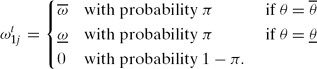
Put simply, these payoffs imply that the effectiveness of a policy might be clearly discerned (and experienced as an added benefit or cost) on adoption, or they might not be so immediately evident. We allow for the possibility that ω ≠ − ω, so that the ex ante expectation of the valence outcome ω1jt may be nonzero.
This characterization of the valence benefit (or cost) as only revealed and experienced with some probability embodies a number of simplifying assumptions.Footnote 7 The draws of ω1jt are independent across both time and states. The revelation probability π is strictly positive and is common knowledge. For π < 1, there could be “false-negative” inferences, because a payoff of zero does not establish the unknown policy's type. However, “false positives” cannot occur, because a payoff of ω or ω automatically implies that policy 1 is of type θ or θ, respectively. Combined with the perfect observability of valence outcomes, the model provides a tractable (if somewhat restrictive) framework for solving the inference problems of potentially large numbers of policy makers.Footnote 8
We assume that the spatial and valence components affect a policy maker's utility function in an additive manner.Footnote 9 In each period, policy maker Sj receives the following utility from the outcomes in his or her jurisdiction:

where u: + → − is continuous, strictly concave, and decreasing (e.g., the commonly assumed quadratic loss function), and z j ∈ is Sj's ideal point. For convenience, and without loss of generality, we spatially order the policy makers, such that z j′ ≤ z j″ for any j′ < j″.
Sequence and Solution Concept
Nature begins the game by choosing the type θ for policy 1. The game sequence for each period is as follows:
1. Each state Sj simultaneously chooses policy p jt.
2. Nature reveals the chosen policy's valence outcome ωijt for p jt = i for each state Sj.
As is common in games of information revelation, we derive perfect Bayesian equilibria in pure strategies. Let H represent the set of all game histories, and h a generic element thereof. In addition, let H 1 represent the set of all one-period histories (consisting of each state's policy choices and the associated set of possible valence outcome realizations). The equilibrium consists of a strategy pair for each Sj, {p j1, p j2}, where p j1 ∈ {1,2} and p j2 : H 1 → Δ({1,2}) maps the period 1 game history into a period 2 policy choice. In the game's pure strategy equilibrium, we assume that policy makers break ties in favor of policy 2 where applicable.
For each history, policy makers also have beliefs about the probabilities of the unknown policy's type. Because all payoff realizations are observable, policy makers share common beliefs.Footnote 10 Thus, let ρ(h) denote the probability that policy 1 is of type θ given the information revealed to date (where the initial beliefs with no information being revealed are assumed to be ρ(∅) = ρ).
Preliminary Developments
We begin with two preliminary developments that are used throughout the article. First, a central feature of the model is that the information available to policy makers in period 2 is endogenous. State policy makers update their beliefs over the unknown policy's type through the period 1 policy choices using Bayes' rule. Suppose that k policy makers choose policy 1 in period 1. By (1), it is clear that if, under history h, ω1j1 = ω for any policy maker, then ρ(h) = 1. Likewise, if ω1j1 = ω for any policy maker, then ρ(h) = 0. Otherwise, in the event that all k trials of policy 1 result in a payoff of zero, Bayes' rule yields:

Thus, k valence outcomes of ω1j1 = 0 out of k choices of policy 1 reveal no additional information about the type θ. In other words, unless at least one state experiences the policy as particularly effective or particularly ineffective immediately on adoption, state policy makers remain unaware of the effectiveness of the policy.
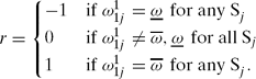
As becomes clear, the existence of only three possible values of ρ(h) greatly simplifies the analysis. It also allows us to adopt the following shorthand for game histories prior to period 2. To summarize the relevant information about experimental results, let r denote whether policy 1 has been revealed to be effective, ineffective, or still unknown:
Second, much of our analysis is based on the location of “cut points” on , which partition states by ideal points. The cut points are used both to identify short-term assessments of each policy's expected value in a single period and to characterize over-time strategic assessments of the expected utility of experimentation. To construct these cut points, it will be convenient to define the expected value of policy 1's valence component for a single period as:

This is the probability of policy i's effectiveness multiplied by the expected valence conditional on being effective, added to the analogous term for ineffectiveness. Note that under our payoff assumptions, policy 2's valence is known and normalized to zero.
It is clear then that, given beliefs over each policy's type ρ(h), state Sj prefers policy 1 over policy 2 in the short term (based on the current period alone) if:

Intuitively, Sj's current-period ranking of two policies is determined by the distance between their policy components, adjusted for uncertainty over the policies' valence types. This determines a unique cut point c(h) satisfying:

Note that if μ(ρ(h)) = 0 (i.e., neither policy has an expected valence advantage), then c(h) = x 1/2 and Sj simply prefers the “closer” policy. As ρ(h) increases, policy 1 becomes more desirable. To see this, observe that an increase in ρ(h) increases μ(ρ(h)) and, in turn, c(h) as well. This expands the set of possible policy makers who would prefer policy 1 to policy 2. For sufficiently large ρ(h), it is possible that c(h) > 0, and thus even a policy maker with ideal point at 0 might prefer policy 1 to policy 2.
These cut points establish the desirability of policy 1's immediate payoff relative to that of policy 2 for each policy maker. Because u(·) is strictly concave, it follows from (6) that regardless of the game history h, each player's relative expected utility for choosing policy 2 (instead of policy 1) is strictly increasing in his or her ideal point z j. Because Sj is indifferent between the policies when z j = c(h), any player with ideal point greater than z j must receive higher expected utility from policy 2, and any player with ideal point less than z j must receive higher expected utility from policy 1. Thus, in period 2, each Sj will prefer policy 1 to policy 2 if and only if z j < c(h).
The following lemma summarizes the period 2 policy choices by rewriting them in terms of the information revealed to policy makers based on first-period policy choices. The result follows directly from the preceding discussion and is thus presented without formal proof. Since policy 2 has a valence of zero for all h, it will be convenient to adopt the following simplifying notation. Let c = c(h) when r = 1, c = c(h) when r = −1, and c = c(∅), thus characterizing the single-period cut points between policies 1 and 2 when policy 1 is effective, ineffective, or unknown, respectively.
Lemma 1. (Period 2 Policy Choice).
![$$
p_j^{2*} = \left\{
\begin{array}{ll}
1 & \mathrm{if~} z_j < \underline c, \mathrm{or~} z_j \in [\underline c, c)
{\hbox{\rm{~and~}}} r > -1, \\[6pt]
& \quad {\hbox{\rm{or~}}} z_j \in [c, \overline c) {\hbox{\rm{~and~}}} r = 1 \\[6pt]
2 & {\hbox{\rm {otherwise}}}.
\end{array}\right.
$$](https://static.cambridge.org/binary/version/id/urn:cambridge.org:id:binary:20151024011004486-0406:S0003055408080271_eqnU1.gif?pub-status=live)
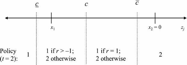
Policy makers select ideologically close policies, but also account for expected valence values. Because x 1 < 0, we may illustrate the result by labeling policy 1 as the “leftist” policy relative to policy 2, as shown in Figure 1. An extreme leftist policy maker will adopt policy 1 regardless of its effectiveness. A slightly more moderate policy maker will adopt policy 1 unless it has been found to be ineffective. Still more moderate policy makers adopt policy 1 only if it were found to be effective, thus possibly abandoning their first-period choice of policy 2. Rightist policy makers always choose policy 2 because of ideological proximity.
Second-Period Policy Choices, Based on Ideology and Information

THE DECISION-THEORETIC MODEL
As established in Lemma 1, policy makers in the second period simply balance each policy's ideological proximity and effectiveness. Fully characterizing policy maker strategies requires also that first-period choices be derived. These decisions are more complex because they incorporate anticipated second-period choices, which depend on information revealed through first-period policy adoptions. Moreover, the value of policy experimentation depends on how much information could be gleaned from other states' experiments.
In this section, we set aside this latter concern and derive the first-period strategies in a decision-theoretic version of the model. Here, any given policy maker, S, acts independently of others, so we suppress notation for the other jurisdictions j. This case is equivalent to a single centralized policy maker or, more interestingly, to a myopic world in which each state acts independently of one another. It therefore serves as a benchmark against which we can compare the learning-based game-theoretic model of the next section. The first-period strategies in this model share many of the complexities of the game-theoretic model, but with the key difference that learning takes place entirely within one state.
The main complexity in calculating S's first-period policy choice is that S must take into account the “option value” of experimenting with an uncertain policy. To gain some intuition, consider the different possible spatial preferences of the state policy maker. The simplest cases involve relatively extreme policy makers. A rightist policy maker with ideal point z ≥ c prefers policy 2 because it yields a higher utility than even an effective policy 1, and S therefore chooses policy 2 in both periods. A leftist policy maker with z ≤ c prefers the expected value of the unknown policy 1 to that of the known policy 2. As a result, S experiments with policy 1 in period 1. If, in addition, z ≥ c, then S switches back to policy 2 in period 2 if policy 1 is found to be ineffective (i.e., r = −1). But if z < c, then S keeps policy 1 regardless of any revealed information.
The most interesting case arises where S's ideal point lies between these clear choices (c < z < c). Here, S prefers policy 2 over an unknown policy 1 based on first-period utilities only. However, experimenting with policy 1 provides an additional learning value: if found effective, it will be retained in the second period, yielding a higher overall utility. In this region, S weighs the expected utilities from (1) experimenting with policy 1 and switching to policy 2 unless policy 1 is found to be effective, against (2) staying with policy 2 in both periods. This trade-off also depends on S's spatial distance from the two policies. Formally, S experiments with policy 1 if and only if:

This equation helps us discover the range of policy makers for whom experimentation is preferred. For the rightmost policy maker in this region (at z = c), S has no incentive to experiment with policy 1, because the policy maker would be indifferent between the two policies even if θ = θ were known with certainty. In contrast, for the leftmost policy maker in this region (at z = c), S will definitely experiment with policy 1, as its expected period 1 payoff equals that of policy 2, and there is an informational benefit to experimenting. Specifically, if found effective, that good policy (and its higher utility) can be experienced for two periods, whereas ineffective policies can be abandoned and are thus experienced for only one period.
Let e be the experimental cut point, or the ideal point for which S is indifferent between policy 2 and experimenting with policy 1. Manipulating (8), e satisfies:

This cut point e is unique and satisfies e ∈ (c, c). By the same argument as was used for the nonexperimental cut points, the strict concavity of u(·) implies that S's best response is completely characterized by the location of z relative to e. S chooses policy 2 if z ≥ e. He or she experiments with policy 1 if z < e and stays with policy 1 if it is found to be effective (r = 1); otherwise, he or she switches to policy 2 in the second period.
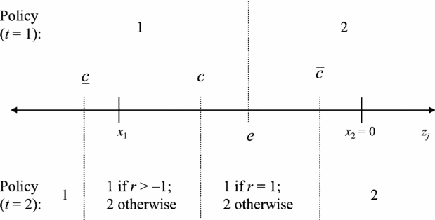
Putting the subcases together, we see that experimentation is monotonic in preferences---a policy maker to the left of the experimental cut point e chooses policy 1 in period 1, but her willingness to stay with policy 1 in the second period varies with both z and r, as illustrated in Figure 1. It is also affected by the degree to which state policy makers value the future because (9) implies that higher values of δ expand the set of ideal points for which experimentation would be desirable.
Proposition 1 formally establishes the equilibrium of the decision-theoretic case.
Proposition 1. (Nonstrategic Experimentation). In period 1,
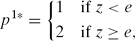
and period 2 strategies are given by Lemma 1.
Proof. All proofs are in the Appendix.
Figure 2 illustrates these results by adding the experimental cut point and first-period strategies to the second-period choices of Figure 1.
Policy Choices Based on Ideology and Information

The intuition of this model is that, although policy choices correspond to preferences along the spatial dimension, they are also affected by the presence of an unknown valence effect. This may give a policy maker an incentive not to choose the policy with the highest immediate payoff. In particular, if his or her ideal point lies in the interval [c, e), he or she forgoes a higher immediate payoff from policy 2 to see if policy 1 is effective. This allows him or her to make a better, more informed second-period choice.
The comparative statics on the experimental cut points follow intuitive patterns. For example, states across a broader range of ideal points are willing to experiment with policy 1 if it is more likely to be effective (ρ increasing) or if it has higher expected valence benefits (ω − ω increasing). There is also more experimentation when the value of the future is greater (δ high) because of the larger potential benefit from learning about the policy's effectiveness. These features of the learning process also hold in the game-theoretic model, to which we now turn.
THE GAME-THEORETIC MODEL
The most intriguing result from the decision-theoretic model is that moderate policy makers in the first period try new policies partly for the learning benefit that allows a better second-period decision. This incentive appears in the game-theoretic model as well. However, now learning can be accomplished by watching the experiments of others as well as by conducting one's own experiment. If other states try a new policy, then the marginal benefit from experimenting is diminished relative to an environment in which experiments are unobservable. Because of this lower value from experimentation, some policy makers who would have adopted an unknown policy in the decision-theoretic model now stay with the safe known policy, essentially free-riding on the experiments of others. Thus, the derivation of the equilibrium strategies resembles that of the previous section, but with the exception that the experimental cut point now depends on other states' actions.
A Simple Example
To see how the presence of multiple experimenters affects policy choice, suppose that there are two policy makers, one of whom chooses policy 1 in the first period. How does this choice affect the incentives of the other state, Sj, in the key potential experimentation region, where c < z j < c? Now policy 1's type θ will be revealed with probability π even if Sj does not choose policy 1. Recall that ρ is the ex ante probability of a high type. The revelation of the high type occurs with probability ρ(1 − (1 − π)2) if both states choose policy 1, and with probability ρπ if there is one experimenter. The revelation probabilities are important because Sj will only choose policy 1 in the second period if it has been proven effective. Analogously to (8), Sj will prefer experimenting with policy 1 over choosing policy 2 if and only if:
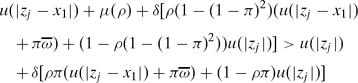
The first part of this expression is the expected utility from choosing policy 1 in the first period and keeping that policy if it is revealed to be effective by either experimenter; otherwise, policy 2 is returned to in the second period. That overall expected utility is compared to the expected utility of choosing policy 2 initially, and only switching if the other state's experiment proves effective. Simplifying this equation, we obtain:

Let e(1) denote the value of z j satisfying (11) with equality. This is the experimental cut point between policies 1 and 2 when one other state experiments with policy 1. Analogously with (9), Equation (11) implies that Sj prefers policy 1 to policy 2 if z j < e(1). A comparison of (9) with (11) reveals the effect of the additional experimenter. The only difference in (11) is that the last terms of the numerator and denominator of the right-hand side are multiplied by (1 − π). This decreases the value of the right-hand side, which is the policy-utility differential between policies 1 and 2 required to induce experimentation.
Comparing Equations (9) and (11) also allows us to establish the relative positions of e and e(1). Because u(|z j|) − u(|z j − x 1|) is increasing in z j, the lower value of the right-hand side of (11) in comparison to (9) implies that e(1) < e. Moreover, e(1) > c because any policy maker for which z j = c must strictly benefit from experimenting. Thus, the presence of a single experiment with policy 1 reduces the set of other policy makers who would experiment with policy 1 from those with z j < e (as in the decision-theoretic model) to those with z j < e(1).
Main Results
This example generalizes to larger numbers of policy makers. Extending the notation for experimental cut points, let e(k) be the value of z j such that policy maker Sj is indifferent between policies 1 and 2 in period 1, given that k other policy makers experiment with policy 1. Given optimal period 2 strategies, all policy makers with ideal points to the left of e(k) prefer policy 1, and those to the right prefer policy 2. We continue to use e to denote e(0). The following result establishes the important properties of experimental cut points for all configurations of experimenters.
Lemma 2. (Experimental Cut Points with Multiple Players). For all k ≥ 0, there exists a unique experimental cut point e(k) ∈ (c, c). The cut point is decreasing in k: e(k + 1) < e(k).
This lemma is useful for developing the intuition for policy makers' strategies. Given any number of experimenters with policy 1, there is a unique experimental cut point that can identify period 1 policy choices. By suitably modifying (10), the equation characterizing e(k) becomes:

The location of the cut point implies that some policy makers to the right of c would be willing to sacrifice some expected utility in period 1 in order to benefit from the possible later adoption of an experimental policy. However, additional experiments with policy 1 will reduce the set of policy makers willing to experiment with that policy relative to policy 2. As with (9), (12) implies that the set of experimenters expands as δ increases.
In equilibrium, the strategies of policy makers who are sufficiently predisposed toward policies 1 or 2 do not change from those in Proposition 1. However for other policy makers, strategies will differ from those of Proposition 1 because the location of the experimental cut point now endogenously depends on one another's choices.
Where exactly the experimental cut point is located can be understood through the following intuition. Suppose that there are k′ policy makers to the left of e. By Lemma 2, there are then no more than k′ policy makers to the left of e(1), and still fewer to the left of e(2). We continue moving to the left until reaching e(k* − 1), the farthest experimental cut point with at least k* policy makers to its left. Given that the k* leftmost policy makers experiment with policy 1, no others would adopt policy 1 in period 1. The remaining legislators (i.e., those with ideal points to the right of z k*) choose policy 2 in period 1.Footnote 11 Compared to the illustration in Figure 2, the first-period choices are thus divided into two regions at z k*, to the left of e(k* − 1), rather than by e from the decision-theoretic case.
Using this approach to construct a pure strategy equilibrium by iteration results in the following proposition. The construction ensures that all sufficiently “leftist” policy makers choose policy 1 in the first period, and all others choose policy 2.
Proposition 2. (Strategic Experimentation). There exists a pure strategy equilibrium characterized by k* = max{k | z k < e(k − 1)}, where in period 1:
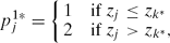
and period 2 strategies are given in Lemma 1.
The equilibrium constructed in the proof of Proposition 2 may not be unique. However, when they exist, the alternative pure strategy equilibria are constrained by the experimental cut points to be very similar to the one constructed here. To see this, consider the set of policy makers whose ideal points fall in the interval (e(k*), e(k* − 1)). If in equilibrium  * > 0 policy makers in this interval choose policy 1, then it is also an equilibrium for any combination of * policy makers in this interval to choose policy 1.Footnote 12 The reason is that, within this interval, all policy makers' induced preferences are essentially identical: given k* − 1 other experimenters, they are each willing to choose policy 1. Proposition 2 selects the simplest such equilibrium, which lets the leftmost of these policy makers choose policy 1. This also happens to be the equilibrium that maximizes aggregate welfare because the leftmost policy makers in this interval receive (slightly) more utility from that policy. The other equilibria are sufficiently similar that relying on one of them instead would not affect the empirical implications discussed later in this article.
Mixed strategy equilibria may also exist in this model. As our preceding discussion established, for a wide range of ideal points, policy makers must choose pure strategies because their preference for one policy over another will not depend on the number of experimenters. But for policy makers with ideal points in (c, c), the decision to experiment depends more generally on the expected number of other experimenters, which may be noninteger valued under mixed strategies. A policy maker whose ideal point exactly equals an experimental cut point will be indifferent between policies, and can therefore mix. Interestingly, because e(·) is decreasing in the number of experimenters, this implies that a mixing policy maker who is ideologically closer to policy 2 must face a lower number of expected experiments by other players than a mixing policy maker who is ideologically closer to policy 1. Thus, somewhat counterintuitively, we conjecture that states that adopt mixed strategies will be more likely to experiment the further they are from the experimental policy.
The result in Proposition 2 contrasts sharply with that of the decision-theoretic model, in which every policy maker to the left of e experiments in the first period. In any pure strategy equilibrium of the game-theoretic model, the definition of the experimental cut points implies that given k* experimenters, no policy maker with an ideal point in the interval (e(k* − 1), e) would experiment with policy 1. Thus, the range of possible experimenters shrinks when players can learn from one another.
Propositions 1 and 2 allow us to analyze the level of information revelation and comparative policy choices between the independent adoptions of the decision-theoretic model and the learning-based diffusion of the game-theoretic model. The following comments formalize two differences across these models, which are used in the Empirical Implications section.
Comment 1. (Learning and Ideological Sorting). In the game-theoretic model, for all first-period histories h, p j2* = 1 if and only if z j < c(h).
Comment 1 says that ideologically similar states (with the exception of those immediately on either side of the cut point c(h)) have the same induced preferences over policy. This follows directly from the common learning in the game-theoretic model. In contrast, ideologically similar states in the decision-theoretic model will have the same induced policy preferences in period 2 only if they observe identical results within their jurisdictions in period 1. Although ideologically extreme states behave the same way in both models, learning coupled with ideological similarity leads moderate states to adopt more similar policies in the game-theoretic model than absent policy learning.
Comment 2. (Free-Riding and Revelation Probabilities). Due to free-riding, the number of experimenting states and the probability that θ is revealed (to at least one state) is at least as high in the decision-theoretic model as in the game-theoretic model.
This result suggests that, in any given policy area, learning-based policy diffusion should be consistent with lower numbers of initial adopters than would be found without learning, given the same number of states in each model. As intuition would suggest, free-riding in the game-theoretic model reduces the probability of revealing the effectiveness of the unknown policy. If one were to consider different policy areas that varied by ease of learning across states, Comment 2 implies more early experimenters in areas with limited policy learning than in areas where learning (and thus free-riding) is easily achieved.
Policy Window Considerations
Throughout the previous model, we assumed that all states are able to change their policies both in period 1 and in period 2. In reality, we know that opportunities for policy change are not so uniform. “Windows” for the adoption of policy innovations may open up at different times in different states (Kingdon Reference Kingdon1984). We therefore briefly note here how the model could be modified to account for such policy windows. Consider the n states of the model to be only a subset of all states. Now, we add N ≥ 1 more states S′1, . . ., S′N that, for whatever reason, do not have an open policy window in period 1. How would they behave in period 2?
The answer depends on whether learning takes place across the states. Absent learning, these states with a newly opened policy window and no information yet revealed will adopt policy 1 if they are located to the left of cut point c and will adopt policy 2 if they are to the right of c. If learning is possible, however, these policy makers take the revealed information into account in choosing their policies, as detailed in Lemma 1. Note that these decisions do not rely on the experimental cut point e because these states did not have an open policy window in which to experiment.
Although thus adding little complexity to the previous findings, the consideration of policy windows is nevertheless valuable in discerning patterns between the decision-theoretic and game-theoretic versions of the model. For example, absent policy windows, a new adoption of experimental policy 1 in period 2 would only occur through learning in the game-theoretic version. In the real world, states adopt policy innovations at different times. Scholars should not simply see the temporal spread of such policies as evidence of learning-based policy diffusion. Independent adoptions by states with different opportunities for change over time would also produce a spread of policy adoptions, as indicated here, simply because of differences in when their policy windows open.
To discern whether adoptions are based on learning or on independent decisions, scholars must look beyond simple over-time policy changes. Instead, evidence of free-riding, of adopting successful policies, or of making decisions based conditionally on which other states have kept or abandoned new policies will be useful to explore whether learning-based policy diffusion is occurring.
Multiple Unknown Policies
The results of the previous model lay the groundwork for numerous empirical implications. However, one perhaps crucial simplifying assumption is the limitation to one unknown and one known policy. In the policy world, there are often competing policy ideas, each with unknown effects. A key question, then, is whether our results are affected by the presence of more than one experimental policy.
Elsewhere, we consider an extension of the model that features two unknown policies, one on each ideological side of x 2.Footnote 13 The analysis of this model is complicated by the fact that “moderate” policy makers may plausibly choose from up to three policies, depending on the experimental results of period 1. Thus, equilibrium strategies depend on not one but three cut points. In this environment, pure strategy equilibria are difficult to characterize because the technique used to prove Proposition 2 may not yield an equilibrium. However, mixed strategy equilibria exist and share many characteristics of the equilibria identified in our baseline model. As in the two-policy model presented previously, (1) similarly positioned states adopt similar policies; (2) the ideological sorting of Comment 1 more cleanly separates states in the second period of the game-theoretic model due to identical learning; and (3) free-riding is only evident in the game-theoretic model, with a larger range of free-riding when there are more states to free-ride on.
EMPIRICAL IMPLICATIONS
Having derived the basic features of both the decision-theoretic and the game-theoretic models, we can now assess whether scholars have been looking in the right places for evidence of learning and policy diffusion. Put simply, would we expect similar behavior in environments with and without communication and learning externalities across jurisdictions? Has behavior that could have arisen from the decision-theoretic model been heralded as evidence of policy diffusion?
The predictions of the decision-theoretic and game-theoretic models are similar in many ways. Most important, in both models, similar states are expected to adopt similar policies. Throughout the previous models, we used the term “ideology” to characterize states' similarity to one another in the one-dimensional space. In reality, that location could capture anything that affects a state's propensity to choose one policy over another. Although political ideology may play such a role, so too would state demographics, interest group involvement, economic circumstances, and numerous other considerations. Importantly, both with and without learning, states that are highly predisposed toward experimental or nonexperimental policies will adopt them in both periods. More “moderate” states may experiment initially, but their subsequent choices will depend on the experimental results. “Leaders” in both the decision-theoretic and game-theoretic models will be those similar states that are most highly predisposed to adopt the policy, with later adopters being less predisposed initially (as in the game-theoretic model) or simply having a later policy window open up (in either model).
Unfortunately, these similarities mean that much of the empirical work to date has not adequately distinguished learning-based policy diffusion from myopic individual adoptions. In the introduction, we noted five types of evidence that scholars typically offer in support of policy diffusion. Because each emerges not only from the learning-based game-theoretic model but also based on the independent actions of the decision-theoretic model, these earlier findings cannot be seen as strong evidence in support of learning-based policy diffusion. To be more specific, first, Walker's (Reference Walker1969) leader states appear in both models because some states are more predisposed to adopt policy changes than are others. Second, Gray's (Reference Gray1973) S-shaped “diffusion curves” could arise from individual states' policy windows opening at about the same time because they face similar policy problems.Footnote 14 Third, if geographically neighboring states share ideological positions or other similarities that predispose them to favor a particular policy change over the status quo, they would be more likely in both the decision-theoretic and game-theoretic models to adopt similar policies at the same time. Fourth, noncontiguous and yet demographically, ideologically, or otherwise similar states likewise would adopt the same policies at similar times in both the decision-theoretic and game-theoretic models. Fifth and finally, assuming strong policy advocates or entrepreneurs could affect policy makers' preferences (in ways consistent with current understandings of interest group politics), such efforts would result in an increased likelihood of policy adoption with or without actual learning-based diffusion.
In short, many of the main approaches used to study policy diffusion do not meet the standard raised here of presenting phenomena emerging from the game-theoretic learning model and not from the decision-theoretic model of individual adoptions. We are not suggesting, however, that policy learning is absent from the decision-making processes of politicians and bureaucrats worldwide. Rather, we argue that scholars must redirect our efforts toward providing evidence that distinguishes between policy diffusion and myopic choice. The models presented here suggest multiple ways of doing so. We briefly raise four differences between the decision-theoretic and game-theoretic versions of our model, noting how empirical tests based on these differences could be constructed.
First, unsurprisingly, increased adoption following evidence of policy success elsewhere emerges only in the game-theoretic model. Straightforwardly, then, scholarship providing evidence of a greater likelihood of policy adoption given earlier effectiveness elsewhere would lend convincing support to the concept of learning-based policy diffusion. Although the idea of policy success being relevant to diffusion is hardly new (Brandeis Reference Brandeis1932), and although studies focusing on such wide-ranging behaviors as airplane hijacking (Holden Reference Holden1986) and coal mining strikes (Conell and Cohn Reference Conell and Cohn1995) have illustrated success-based learning, similar systematic studies of learning from effective policies had been surprisingly absent in the policy diffusion literature until quite recently. Perhaps part of this hesitance arose from the need to confront and overcome a number of methodological issues in studying the effect of policy successes across states (e.g., Manski Reference Manski1993). However, some promising initial steps have been taken in this direction. Volden (Reference Volden2006), for example, devises a dyad-based variant on the classic event history analysis, uncovering learning-based diffusion in the Children's Health Insurance Program across the American states. Meseguer (Reference Meseguer2006) illustrates how to incorporate measures of policy success into a more standard event history analysis framework.
A second potentially fruitful empirical strategy moves away from reliance on direct evidence of policy success. In many cases, researchers lack adequate data regarding the direct effectiveness of new policies.Footnote 15 For example, Boehmke and Witmer (Reference Boehmke and Witmer2004), Berry and Baybeck (Reference Berry and Baybeck2005), and Shipan and Volden (Reference Shipan and Volden2008) all seek to disentangle learning from other potential mechanisms of policy diffusion. They rely on the existence over time of the policy elsewhere (typically among geographic neighbors), with the assumption that a greater exposure to the new policy creates a more substantial opportunity to learn about its characteristics, including its effectiveness.
As noted, researchers should be cautious to not simply accept the adoption of similar policies by neighbors as evidence of policy diffusion. However, distinctions between our decision-theoretic and game-theoretic models offer a path forward even in the absence of direct measures of policy effectiveness. Consider, for example, the policy choices of the leftmost and rightmost states in our model. Due to their extreme predispositions, these states keep their first-period policy for the second period, regardless of internal or external evidence of the policy's effectiveness. More moderate states, however, would abandon an ineffective policy. Thus, the longevity of moderate states' policy choices is more informative than any behavior of extreme states. Observing empirically that the longevity of policy adoptions in other states matters for policy adoption, and matters differentially based on the propensity of those states to keep the policy even if ineffective, would thus be strong evidence of learning-based policy diffusion.
Notice that this conditional-effect prediction differs from that of previous studies relying simply on the proportion of similar states that had already adopted a policy. Revisiting our example of antismoking restrictions from the introduction, consider a ban on smoking in restaurants and bars that tends to be supported by liberal policy makers. The decision-theoretic model predicts that liberal states will adopt the policy and conservative states will not. Evidence of earlier adoptions by other states should be irrelevant. However, because states in the real world may vary in the timing of policy windows opening due to policy crises or political opportunities, spurious evidence of adoption based on prior adoption by ideologically similar states may emerge. Liberal states would adopt the earlier bans in other liberal states, and conservative states would “mimic” one another in not adopting bans. The resulting pattern would resemble one in which states adopted policies according to ideological similarity (e.g., Grossback, Nicholson-Crotty, and Peterson Reference Grossback, Nicholson-Crotty and Peterson2004), but it arises simply in a decision-theoretic model with differing policy windows across states.
In contrast, the game-theoretic model suggests a more systematic and conditional pattern to the effect of previous adoptions. Liberal states will of course adopt the policy regardless of other states' experiments, and conservative states will not adopt the policy regardless of others. However, depending on their positions relative to the new policy, moderate states either will adopt the policy initially but will abandon it if not proven broadly effective, or they will adopt the policy only if others establish its effectiveness. Thus, the game-theoretic model predicts a more conditional pattern of adoption by similar states.Footnote 16 This pattern would not arise from variations in policy window openings and separates the analysis based on our model from previous similar-states analyses.
To test for learning in the absence of direct measures of success, researchers could incorporate interactions between state (moderate) ideology and the (moderate) ideology of previous adopters into standard event history analysis models. Many moderate states will not adopt the policy absent evidence of success, and researchers can detect that evidence via the longevity of policy maintenance by other moderate states that would have otherwise abandoned an ineffective policy. Moreover, such tests need not be based solely on ideology, but on any variable affecting the propensity of policy adoption, as discussed previously. Policy duration--based learning is more likely from states that adopted the policy despite a lower propensity for adoption than from the high-propensity adopters that would keep the policy even if ineffective.
Third, stepping away from the concept of policy adoption, patterns of policy abandonment also provide an opportunity to distinguish learning-based policy diffusion from independent actions. As noted in Comment 1, the game-theoretic model features ideological sorting. Specifically, because all states receive the same information about the policy successes of one another, all moderate states would abandon the new policy uniformly on evidence of its ineffectiveness. This is in contrast to the decision-theoretic model, in which only one's own experience with the policy is weighed in making subsequent policy choices (and the effectiveness of the policy may not be revealed after experiencing it only for one period).
Empirically, consider once again an antismoking policy that could be less beneficial than expected, due to public backlash, declines in business in nonsmoking restaurants and bars, or insufficient effects on teen smoking rates, for example. If states do not learn from one another, evidence of this particular policy being ineffective would emerge one by one across the states, perhaps a number of years after the policy's adoption. If states do learn from one another, however, once evidence of the policy's downside emerges in one state, that evidence affects the other states' decisions. An empirical examination of policy abandonment based on the decision-theoretic model would predict the abandonment to be a function of years since the policy was adopted in the given state, in order to capture the time until its downside is discovered within that state. In contrast, evidence of abandonment when others are similarly abandoning the policy, with a temporal cluster of ideologically (or otherwise) similar states all abandoning their policies at the same time, would be consistent with cross-state learning, rather than with individual experiences.
Fourth, another striking feature of the game-theoretic model that was absent from the decision-theoretic model was the free-riding behavior of states who understood that they could allow other states to experiment with the risky policy and learn from their experiences, rather than taking on the experiment themselves. Thus, finding free-riding behavior with respect to learning would support the game-theoretic model over the decision-theoretic model. However, detecting such free-riding may be a difficult problem. One possibility is to exploit variation in the number of potential experimenters. In the game-theoretic model with just a few states, the informational contribution of each experiment is relatively large. But with more states, Lemma 2 and Comment 2 suggest that the increased level of experimentation due to the high number of extremists would reduce the marginal value of experimentation and allow many policy makers to free-ride. As a result, the ratio of early adopters to total adopters decreases with the number of states in the game-theoretic model, while remaining constant in the decision-theoretic model.
Empirically, one would expect more free-riding in studies of hundreds of local governments than in studies of 50 states, and still less in studies of diffusion across a limited number of countries, such as European Union governments. Returning once more to the antismoking policy area, consider the possibility of intercity learning within each state (e.g., Shipan and Volden Reference Shipan and Volden2008). States such as California have many more cities with populations over 50,000 than most smaller states. All else equal, one would expect intrastate adoptions to exhibit a different over-time pattern, depending on the number of cities.Footnote 17 Where there are many potential experimenters, more free-riding is likely, and therefore, the probability of early adoption compared to later adoption is lower. Given learning across cities within each state, an event history model that incorporates a variable capturing time since first adoption in the state interacted with the number of cities in the state should find a negative effect. This effect would indicate greater hesitance to experiment in larger states, due to free-riding off the information of a larger number (but not proportion) of early adopters.
Many considerations must be weighed as to how to best explore the free-riding concept in any particular policy area. As a quite preliminary test of this free-riding concept, we reran the full model of local antismoking policy diffusion presented in Shipan and Volden (Reference Shipan and Volden2008). In addition to their independent variables, we added a simple variable capturing how many cities (using Shipan and Volden's 50,000 population threshold) were in the state. This approach uncovered systematic evidence of free-riding, even controlling for all other mechanisms of diffusion explored in the original study. Specifically, in the early years of the data set (when less than 10% of the state population was covered by local antismoking restrictions), each additional city in existence in the state is associated with 0.5% lower odds of policy adoption by the city being examined. Consequently, cities in states with few large cities were more than twice as likely to be early adopters of antismoking policies as were the free-riders in California (with 152 cities with populations in excess of 50,000). This effect is not evident for later periods in the data-set, when the consequences of these policies were likely already known and the benefits of free-riding were thus diminished.
In sum, our theory calls for a major shift in the nature of empirical research on policy diffusion. As demonstrated in the simple models of this article, much of the scholarly work seen previously as evidence of policy diffusion could have arisen through independent actions of states that confront common problems at about the same time and only learn from their own experiences. However, by redirecting our efforts toward exploring behavior that emerges only in a cross-state learning environment, we can start to uncover more systematic evidence of when and where learning-based policy diffusion occurs. We suggest that such evidence can be found through studies that focus on policy success, on conditional patterns of policy maintenance and longevity, on policy abandonment, and on free-riding behavior. We believe that these avenues for future research provide a substantial range of possible new approaches through which scholars can analyze policy diffusion.
CONCLUSIONS
Localities, states, and countries have the potential to learn from one another's policy experiments. Whether and when they actually learn, resulting in policy diffusion, remain open questions. We present two models of learning and policy choice, differentiated solely by whether learning takes place across governments or only within governments over time. In so doing, we establish that much of the existing support for policy diffusion could just as easily have been generated through the individual decisions of myopic policy makers unaware of one another's experiences. However, differences between the decision-theoretic and game-theoretic models show numerous ways to proceed in empirical attempts to uncover the extent of learning-based policy diffusion.
Although our main goal in developing these models was to confront the issue of discerning learning-based diffusion from individualized policy choices, the game-theoretic model presented here has the potential to provide even greater insight into the diffusion and learning processes across governments. Due to space considerations, we did not fully report comparative statistics results regarding how such features as policy location, probability of policy success, benefit from policy success, or discounting affect experimentation and policy adoption. Exploring these in greater detail may lend further insights into when and where policy diffusion takes place.
Moreover, the baseline model presented here can be extended in ways that could lead to other theoretical and empirical advancements. For example, this model of learning and policy diffusion may be thought of as representing decentralized policy making in a federal system. A complementary model of centralized policy making would help determine when policy decentralization is desirable (Kollman, Miller, and Page Reference Kollman, Miller and Page2000; Strumpf Reference Strumpf2002). Alternatively, the inclusion of elected policy makers, or those with different time horizons, could better explain how policy diffusion is affected by electoral politics. Costs of switching from one policy to the next could be incorporated to further explore the relationship between free-riding and the hesitance policy makers may feel in adopting new policies that are difficult to reverse. Finally, extending the model beyond two periods or exploring variations in the flow of information between the extreme cases of no transmission and perfect transmission would better approximate real-world decision-making environments. These and other extensions would help provide more solid theoretical ground for future empirical explorations of policy diffusion.
APPENDIX
Proof of Proposition 1. There are three possible realizations of r, which define the cut points (in decreasing order) c, c, and c. These cut points partition the set of ideal points into four segments, which we analyze as follows:
1. z ≥ c: S prefers policy 2 to policy 1 even if r = 1, and therefore chooses policy 2 in both periods: p 1* = p 2* = 2.
2. z < c: S prefers policy 1 to policy 2 even if r = −1, and therefore p 1* = p 2* = 1.
3. z ∈ [c, c): S prefers policy 1 to policy 2 if solely focused on period 1. If r = −1, then the optimal period 2 choice is policy 2; otherwise, he or she prefers policy 1. Clearly, in both periods, S's expected payoff is at least that of choosing policy 2. Thus,

4. z ∈ [c, c): S prefers policy 2 to policy 1 if solely focused on period 1, and would choose policy 1 in period 2 if and only if r = 1. Comparing expected utilities, S chooses policy 1 in period 1 iff (8) holds. Simplifying (8) yields:
(13)The left side of (13) is the expected payoff along the nonpolicy dimension under optimal experimentation. The right side is a weighted difference in utility along the policy dimension; it is continuous, unbounded, and increasing in z. By the results of segments 1 and 3, the expression is satisfied at z = c, but not at z = c. Thus, (13) characterizes a unique experimental cut point e ∈ (c, c), solving (9), such that S experiments with policy 1 if and only if z < e. Thus,



Combining the results of these segments yields the main result.
Proof of Lemma 2. Observe first that for all k, by the argument in the proof of Proposition 1, experimentation with policy 1 cannot be optimal if z j ≥ c, and that experimentation with policy 1 is optimal if z j < c. Thus, it is sufficient to consider only z j ∈ [c, c).
We first show uniqueness. Given that k ≥ 0, other policy makers experiment with policy 1 and that r < 1 results in a switch to policy 2, Sj experiments with policy 1 iff:
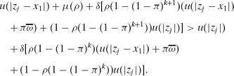
Simplifying yields:

By the strict concavity of u(·), u(|z j|) − u(|z j − x 1|) is continuous, unbounded, and strictly increasing in z j, and the right-hand side of (15) is constant. Thus, there is a unique e(k) ∈ [c, c) satisfying (15) with equality. Sj then prefers experimentation with policy 1 iff z j < e(k).
To show that e(k) > c (and, hence, e(k) ∈ (c, c)), it is sufficient to demonstrate that Sj experiments if z j = c. If z j = c, then in period 1 Sj receives the same expected utility from policies 1 and 2 (i.e., u(|z j − x 1|) + μ(ρ) = u(|z j|)). Rewriting (14) then yields the following condition for experimentation:
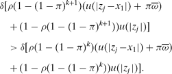
Simplifying yields:

Clearly, δρπ (1−π)k > 0 for all k. By the fact that c < c, u(|z j − x 1|) + π ω > u(|z j|). Therefore, (16) holds for all k.
Finally, to show that e(k + 1) < e(k), it is sufficient to show that the right-hand side of (15) (i.e., the expected policy utility differential required to induce Sj to choose policy 1) is decreasing in k:
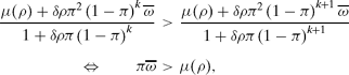
which holds trivially. Thus, e(k) has all claimed properties of an experimental cut point.
Proof of Proposition 2. We construct the equilibrium strategies as follows. At t = 2, the strategies follow directly from Lemma 1. At t = 1, consider first policy makers for which z j < c. By an argument identical to that in the proof of Proposition 1, all such policy makers strictly prefer experimenting with policy 1 to policy 2. Thus, p 1* = 1.
For players for whom z j ≥ c, we consider those players with ideal points z j < c. We assign period 1 experimentation strategies iteratively as follows. Let n 1 be the number of players for which z j ≤ c. Begin by assigning players S1, . . ., Sn 1 to policy 1, and players Sn 1+1, . . ., Sn to policy 2. Let κ serve as a counting variable, with an initial value of n 1. Recall that by assumption, z j is increasing in j. Each stage of the iteration is then:
1. If κ = n or z κ + 1 ≥ e(κ), then the iterative process is complete; let k* = κ.
2. If z κ + 1 < e(κ), then assign Sκ + 1 to policy 1.
3. Increase κ by 1, and return to step (1).
This procedure assigns players S1, . . ., Sk* to policy 1. To show that it converges, note that by Lemma 2, e(k) is decreasing in k and e(k) ∈ (c, c) for all k ≥ 0. Then because n is finite and z k is increasing in k, the iteration clearly terminates at a well-defined k* = max{k | z k < e(k − 1)}. This implies z k* ∈ [c, e(k* − 1)) ⊂ [c, c).
To show that these experimentation strategies are optimal, consider first the policy makers S1, . . ., Sk*. By the definition of e(·), given that k* − 1 other players experiment with policy 1, each of S1, . . ., Sk* choose policy 1 at t = 1. Now consider the policy makers Sk*+1, . . ., Sn. Given that k* players experiment with policy 1, policy 2 is a best response by the definition of e(k*). Because e(k*) is invariant with respect to the number of players choosing policy 2, the strategies of the players assigned to policy 1 remains optimal. Thus, p j2* = 1 if z j ≤ z k*, and p j2* = 2 otherwise.
Proof of Comment 1. This follows immediately from the construction of c(h).
Proof of Comment 2. In the decision-theoretic model, all players for whom z j < e (≥e) choose policy 1 (2) at t = 1. By Proposition 2, in the game-theoretic model, all players for whom z j < e(k*) (≥ e(k*)) choose policy 1 (2). Because k* ≥ 0, Lemma 2 implies e(k*) ≤ e. Thus, the number of players choosing policy 1 at t = 1 is weakly higher in the decision-theoretic model. The result on the probability of revelation follows immediately.



Comments
No Comments have been published for this article.