1. Introduction
1.1. The broader context
Gas bubbles bursting at the surface of a liquid are known, under the appropriate conditions, to eject drops in their surrounding environment. It is not only a fascinating problem per se, but also important to understand for its ubiquitous applications: disease and pathogen transport (Poulain & Bourouiba Reference Poulain and Bourouiba2019), lava bubble bursting (Wilson Reference Wilson1980; Vergniolle & Brandeis Reference Vergniolle and Brandeis1996; Gonnermann & Manga Reference Gonnermann and Manga2007), formation of condensation nuclei (Woodcock et al. Reference Woodcock, Kientzler, Arons and Blanchard1953), champagne aroma transport (Ghabache et al. Reference Ghabache, Liger-Belair, Antkowiak and Séon2016), and broader role in liquid fragmentation (Villermaux Reference Villermaux2007).
In the open sea, such drops are propelled in the atmospheric boundary layer, where they may travel upwards for times much longer than their gravity settling time in a quiescent atmosphere. Constituted of sea water, these spray drops carry salts (among other materials), which remain in suspension in the atmosphere once the liquid has evaporated. In this way, bubbles bursting at the surface of the ocean contribute to sea spray aerosols, whose implication as cloud condensation nuclei has long been established, since the pioneering works of Coulier (Reference Coulier1875) and Aitken (Reference Aitken1880), and later Blanchard (Reference Blanchard1954) and Mason (Reference Mason1971). Their precise chemical composition and role in atmospheric processes remains an active area of research (DeMott et al. Reference DeMott2016; Cochran et al. Reference Cochran, Ryder, Grassian and Prather2017), and requires an understanding of the production processes.
1.2. Sea spray aerosols: the quest for parameterization
One of the related challenges in ocean and atmospheric sciences has long been to parameterize accurately sea spray aerosol production, through the use of a sea spray generation function. Classic sea spray generation functions depend on meteorological parameters, primarily the wind speed (Fairall, Kepert & Holland Reference Fairall, Kepert and Holland1994; Lewis & Schwartz Reference Lewis and Schwartz2004), but significant scatter remains in current formulations, in part due to the large range of scales involved (de Leeuw et al. Reference de Leeuw, Andreas, Anguelova, Fairall, Lewis, O'Dowd, Schulz and Schwartz2011; Veron Reference Veron2015). Sea spray generation is related to surface breaking waves, either directly during wave impact and atomization by wind shear (Veron et al. Reference Veron, Hopkins, Harrison and Mueller2012; Erinin et al. Reference Erinin, Wang, Liu, Towle, Liu and Duncan2019), or through bubble bursting following air entrainment by breaking (Deike, Melville & Popinet Reference Deike, Melville and Popinet2016; Deike, Lenain & Melville Reference Deike, Lenain and Melville2017; Deike & Melville Reference Deike and Melville2018) so that the sea state modulates the droplet production (Lenain & Melville Reference Lenain and Melville2017), together with the precise ocean water temperature and composition (salinity, biological activity, etc.) which will impact interfacial phenomena (Wang et al. Reference Wang2017; Frossard et al. Reference Frossard2019).
1.3. Bubbles at the surface
In this oceanographic context of sea spray production, bubble bursting mechanisms have been singled out and identified, as reviewed by Veron (Reference Veron2015) and illustrated in figure 1. Jet drops are produced when the bubble cavity collapses and forms a vertical upward jet that destabilizes into drops (Blanchard Reference Blanchard1954; Duchemin et al. Reference Duchemin, Popinet, Josserand and Zaleski2002; Ghabache et al. Reference Ghabache, Antkowiak, Josserand and Séon2014; Gañán-Calvo Reference Gañán-Calvo2017; Brasz et al. Reference Brasz, Bartlett, Walls, Flynn, Yu and Bird2018; Deike et al. Reference Deike, Ghabache, Liger-Belair, Das, Zaleski, Popinet and Séon2018; Lai, Eggers & Deike Reference Lai, Eggers and Deike2018; Berny et al. Reference Berny, Deike, Séon and Popinet2020; Blanco–Rodríguez & Gordillo Reference Blanco–Rodríguez and Gordillo2020). The mechanism concerns mostly small bubbles, when compared to the capillary length  $\ell _c = \sqrt {\gamma /\rho g}\ (= 2.7$ mm in water), with
 $\rho$ the water density,
 $\gamma$ the air–water interfacial tension and
 $g$ the gravitational acceleration (Jurin Reference Jurin1717). It is thus dominated by capillarity, and occurs on the inertio-capillary time scale
 $\tau _c = \sqrt {\rho d^3/\gamma }$, with
 $d$ the bubble diameter.
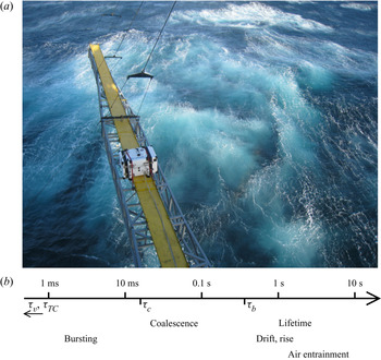
(a) Photograph taken after a large breaking event from R/P FLIP during the SoCal 2013 programme off the coast of southern California in November 2013. Bubble activity at the ocean surface is clearly visible after the breaking event. (b) A schematic of the wide range of time scales involved in bubble processes at the surface estimated for a typical bubble size  $d = \ell _c$, the capillary size. The visco-capillary time
 $\tau _v = \mu d/\gamma \simeq 0.04$ ms and cap retraction time
 $\tau _{TC} = d/\sqrt {2\gamma /\rho h} \simeq 0.1$ ms are too short to appear in the diagram. Time
 $\tau _c = \sqrt {\rho d^3/\gamma } \simeq 17$ ms is the inertio-capillary time, appearing in the reorganization of the bubble cavity at bursting and coalescence. Time
 $\langle \tau _s \rangle \propto \tau _v \sqrt {d/\ell _c} \simeq 0.7$ s is the typical surface bubble lifetime predicted by Poulain et al. (Reference Poulain, Villermaux and Bourouiba2018). Rising and drifting are estimated from a typical rise velocity of 0.1 m s
 $^{-1}$ over distances of 0.1–1 m.

Film drops are generated by the puncture, retraction and destabilization of the thin cap of mainly large bubbles with  $d > \ell _c$ (Blanchard & Syzdek Reference Blanchard and Syzdek1988; Spiel Reference Spiel1998; Lhuissier & Villermaux Reference Lhuissier and Villermaux2012; Poulain, Villermaux & Bourouiba Reference Poulain, Villermaux and Bourouiba2018). Capillarity once again dominates the dynamics, by setting the retraction velocity of the film:
 $V = \sqrt {2\gamma /\rho h}$ (Taylor Reference Taylor1959; Culick Reference Culick1960) and thus the relevant time scale
 $\tau _{TC} = \sqrt {\rho h d^2/\gamma }$, with
 $h$ the cap film thickness.
Figure 1 illustrates bubble plumes generated by breaking waves at the ocean surface, seen from above. The presence of whitecaps indicates that the bubbles, once they have reached the surface, do not burst immediately, but instead spend some time there, much longer than the scales  $\tau _c$ and
 $\tau _{TC}$. Figure 1(b) shows the different time scales involved on a single schematic scale, starting with the fast bursting and coalescence scales, driven by capillarity (10 ms and below; Vella & Mahadevan Reference Vella and Mahadevan2005; Paulsen et al. Reference Paulsen, Carmigniani, Kannan, Burton and Nagel2014), up to the slower scales of bubbles rising in the plume (Clift, Grace & Weber Reference Clift, Grace and Weber1978), drifting at the surface (Deike et al. Reference Deike, Melville and Popinet2016) and lifetimes (Poulain et al. Reference Poulain, Villermaux and Bourouiba2018) from 0.1 s and longer. Surface bubbles thus evolve on a wide range of time scales, all of which have to be taken into consideration for a complete understanding, as well as accurate parameterizations, of sea spray production.
1.4. Surfactants and the physicochemistry of the interface
The behaviour of the ocean surface, partly covered by a biofilm, can be modelled with the help of surfactants, following the approach of Wurl et al. (Reference Wurl, Wurl, Miller, Johnson and Vagle2011) and benefiting from decades of research on the physicochemistry of liquid–gas interfaces. Surface-active materials are known to modify the static and dynamic behaviours of a water–air interface in many different ways. Of primary interest to us, they favour foam stability by delaying or preventing bubble coalescence (Garrett Reference Garrett1967; Oolman & Blanch Reference Oolman and Blanch1986; Weaire & Hutzler Reference Weaire and Hutzler1999; Stevenson Reference Stevenson2012; Cantat et al. Reference Cantat, Cohen-Addad, Elias, Graner, Höhler, Pitois, Rouyer and Saint-Jalmes2013; Langevin & Rio Reference Langevin and Rio2015) and increasing bubble lifetime (Modini et al. Reference Modini, Russell, Deane and Stokes2013; Poulain et al. Reference Poulain, Villermaux and Bourouiba2018). They also readily dampen capillary waves (Franklin Reference Franklin1774; Liu & Duncan Reference Liu and Duncan2006) and ‘rigidify’ interfaces (Levich Reference Levich1962), among important features still under active scrutiny.
In the oceanographic context, the composition of the sea-surface microlayer plays a major role in the later composition of aerosols, hand in hand with spray production mechanisms (Modini et al. Reference Modini, Russell, Deane and Stokes2013; Collins et al. Reference Collins2014; Cochran et al. Reference Cochran, Ryder, Grassian and Prather2017; Wang et al. Reference Wang2017). Multiple approaches have attempted to describe the role of the physicochemical parameters in bubble bursting and the subsequent droplet and aerosol production, with large variations in protocols and results sometimes contradicting each other. Frossard et al. (Reference Frossard2019) describe a bubble plume simulator, taken aboard a cruise to produce an abundant sea spray with real-time ocean conditions, and observe an increase in spray production with increased biological activity and inferred surfactant conditions. The laboratory experiment of Modini et al. (Reference Modini, Russell, Deane and Stokes2013), which investigates the effect of surfactant on saltwater single bubble bursting, yields the opposite conclusion that the aerosol production efficiency is decreased by the addition of surfactant. The approach by Prather et al. (Reference Prather2013) intends to bring the ocean, with all its complexity, into the laboratory, with a controlled blooming experiment, along with carefully injected bubbles, to observe the associated aerosol production. In this case, the large variations of biological activity during the bloom went almost undetected in the sea spray properties (aerosol numbers and sizes). The problem is certainly complex, as even the major trends seem to remain not perfectly clear, and a physics-based parameterization is still to be unveiled. All three articles finally acknowledge and discuss the likely role of bubble clustering in rafts, or whitecaps, but remain elusive about actual mechanisms (Modini et al. Reference Modini, Russell, Deane and Stokes2013), or applicability of very dense foams to oceanic conditions (Frossard et al. Reference Frossard2019). Numerous other studies have been performed (see for instance the introduction and comparison in Modini et al. (Reference Modini, Russell, Deane and Stokes2013)) but the inclusion of a universal physicochemical control on aerosol production remains an open question.
1.5. A dedicated study of collective surface bubble dynamics in controlled conditions
Therefore, on the one hand, individual bursting mechanisms have benefited over the years from detailed laboratory experiments, high-fidelity simulations and a comprehensive theoretical framework. On the other hand, intense research both on the physicochemistry of interfaces and on the sea surface in the laboratory as well as in the field has highlighted the critical role of surface-active material, whether biological (biofilm) or engineered (surfactants). In between, data that would embrace the full complexity of the problem are hard to acquire and to rationalize according to available physics-based parameterizations.
We present a laboratory study aiming at filling this gap in knowledge, and attempt to quantify the role of collective effects from bubbles assembled at the surface of water. Two complementary set-ups are designed, that altogether fully characterize the dynamical and statistical evolution of bubbles at the surface of water. The experimental facilities allow for a careful control of the underwater bubble plume, characterized by its size distribution and density. Independently from bubble production, we investigate the role of water surface contamination by adding various concentrations of surfactant (sodium dodecylsulphate (SDS) and Triton X-100 (Triton)). We monitor the surface bubble dynamics over time scales nearly covering the range highlighted in figure 1, short enough to capture the dynamics (down to 10 ms), as well as long enough (up to hours) to achieve and study converged statistics.
The paper is organized as follows. We depict the experimental set-ups in § 2: a time-resolved bubble raft decay in § 2.2 and a statistically stationary bubble plume in § 2.3. The dynamics of the bubble raft for increasing levels of surface contamination is first analysed in the freely decaying configuration in § 3, from which global bubble merging and bursting rates are measured for increasing surfactant concentrations. Next, the raft dynamics under a continuous injection of bubbles is described in § 4, where we identify two regimes of collective surface bubble evolution: one featuring relatively clean water, high probabilities of coalescence and short bubble lifetime, and another one with contaminated water, no coalescence and longer lifetime. We characterize the statistics of these regimes in § 5. The findings are finally rationalized in a cellular automaton model in § 6, before conclusions and recommendations are given in § 7.
2. Experimental set-ups
2.1. Surface contamination
We investigate and present in this article the influence of surface contamination by the model surfactants SDS (by Sigma-Aldrich) and Triton (by Sigma-Aldrich) on the behaviour of bubbles at the surface. Surfactants SDS and Triton are chosen as common and well-known anionic and non-ionic surfactants, respectively (Mysels Reference Mysels1986; Fainerman et al. Reference Fainerman, Lylyk, Aksenenko, Makievski, Petkov, Yorke and Miller2009, Reference Fainerman, Lylyk, Aksenenko, Petkov, Yorke and Miller2010). Whether initially solid (SDS) or liquid (Triton), a controlled mass (precision 1 mg) of surfactant is dissolved into water, in concentrations  $c$ smaller than the critical micellar concentration (CMC):
 $c = 0.1$–
 $300$
 $\mathrm {\mu }$mol l
 $^{-1}$ (hereafter
 $\mathrm {\mu }$M), with
 ${\rm CMC} = 8.2$ mmol l
 $^{-1}$ for SDS; and
 $c = 0.25\text {--}50\ \mathrm {\mu }$M with
 ${\rm CMC} = 220\ \mathrm {\mu }$M for Triton. The large volume of water in the main set-up (at least 84 l; see § 2.3) allows for such low surfactant concentrations, and solutions for the raft decay experiment (described in § 2.2) were sampled in situ, scooping the required liquid quantity out of the bath surface. Deionized, clean water at room temperature was systematically used, and atmospheric conditions (temperature, humidity and pressure) were frequently recorded in the course of the experimental runs.
Static surface tension  $\gamma (c)$ is measured by the pendant drop method (Berry et al. Reference Berry, Neeson, Dagastine, Chan and Tabor2015), with the results plotted with respect to the concentration
 $c$ of surfactant in figure 2. Our values are consistent with data tabulated in the literature (Mysels Reference Mysels1986; Fainerman et al. Reference Fainerman, Lylyk, Aksenenko, Makievski, Petkov, Yorke and Miller2009, Reference Fainerman, Lylyk, Aksenenko, Petkov, Yorke and Miller2010). However, note that the static surface tension is not the main control parameter in the context of the dynamical processes of bubbles merging and bursting at a free surface. Instead, we keep the surfactant concentration
 $c$ as the experimental contamination parameter. In particular, below a certain concentration
 $c_0$ and within the pendant drop observation time (typically a few seconds to a few minutes), the static surface tension does not depart significantly from the clean water value
 $\gamma \simeq \gamma _w$ (for a departure of 2 % from
 $\gamma _w$,
 $c_0 \approx 200\ \mathrm {\mu }$M for SDS and
 $c_0 \approx 5\ \mathrm {\mu }$M for Triton). Most interesting behaviours, including the cancelling of coalescence probability between two bubbles (Yang & Maa Reference Yang and Maa1984; Oolman & Blanch Reference Oolman and Blanch1986; Shaw & Deike Reference Shaw and Deike2021), occur below that concentration. Above
 $c_0$,
 $\gamma$ eventually decreases within observable time (a few seconds), a signature of adsorption dynamics of surfactant molecules from the bulk to the surface, triggered by the increase in surface area when creating the pendant drop (Fainerman et al. Reference Fainerman, Lylyk, Aksenenko, Makievski, Petkov, Yorke and Miller2009, Reference Fainerman, Lylyk, Aksenenko, Petkov, Yorke and Miller2010; Cantat et al. Reference Cantat, Cohen-Addad, Elias, Graner, Höhler, Pitois, Rouyer and Saint-Jalmes2013).
Static surface tension  $\gamma$ of solutions of SDS (black,
 $\textrm {CMC} = 8.2$ mM) and Triton (red,
 $\textrm {CMC} = 220$
 ${\mathrm {\mu }}$M) in deionized water, by the pendant drop method. The concentration
 $c_0$ indicates a departure of 2 % from the value in pure water
 $\gamma _w = 72$ mM m
 $^{-1}$, highlighted by the shaded grey area.

2.2. Bubble raft decay
The first experiment, intended to characterize bubble rafts dynamically, is shown schematically in figure 3. A raft of monodisperse bubbles is formed at the surface of a water bath by blowing air underwater at a controlled flow rate through a thin needle ( $q_{v} = {O}(5)$ cm
 $^3$ s
 $^{-1}$; needle inner diameter of 180
 $\mathrm {\mu }$m). The level of water in the container (a Petri dish with diameter of 9 cm and height of 13 mm) is kept slightly above the dish edges, so that the concave meniscus prevents bubbles from accumulating on the sides. As seen in figure 3(b), the typical bubble diameter
 $\langle d_b \rangle = 1.9 \pm 0.1$ mm lies in the millimetric range, and the raft extent does not exceed a third of the dish diameter. Potential influence from the container sides may therefore be safely neglected. For each solution, the experiment is repeated at least 10 times under the same atmospheric conditions (temperature, relative humidity, pressure), with some variability in the number of initial bubbles
 $N_0$. The mean bubble size
 $\langle d_b \rangle$ is not modified by the addition of surfactant (see also § 2.3.2 and figure 6).
Bubble raft decay experiment. (a) Monodisperse bubbles injected by blowing air through a needle. The needle is removed from the field of view prior to triggering image acquisition. (b) A sample image of a raft with  $N = 149$ bubbles, shortly after needle removal (SDS,
 $c = 256\ \mathrm {\mu }$M). Detected positions, sizes
 $d_s$ (white dashed circles) and velocities (red arrows) are overlaid on top of the original image.

Image acquisition, from above, is triggered when the bubbling needle is removed from the bath (and out of the field of view), at a frame rate of 100 Hz, or higher. The bath is illuminated from below with a uniform light-emitting diode panel. On every frame, bubble diameter  $d_s$ and
 $x, y$ position on the water surface are detected unequivocally by intensity thresholding. Individual bubbles are then tracked across frames, giving access to their horizontal displacements and velocities (figure 3b).
In the course of a raft lifetime, bubbles do not only move at the surface, they may also merge, and they eventually burst. Coalescence events are tracked based on bubble volume conservation. At merging, two bubbles  $i, j$ with respective diameters
 $d_i, d_j$ disappear into a newly formed bubble
 $k$, with diameter
 $d_k$. Bubbles are large enough to safely neglect the Laplace pressure contribution differential before and after the coalescence, and volumes
 $d_s^3$ (up to prefactors) add up:
 $d_k^3 = d_i^3 + d_j^3$ (see also § 2.3.1). Figure 4(a) depicts one example of a raft before and after a merging event, highlighting the bubbles involved in the process and the successful detection. Figure 4(b) reconstructs a three-step coalescence tree, leading to the formation of a bubble larger than the injected size
 $\langle d_b \rangle$. This automated processing (bubble detection, tracking and event characterization) allows one to follow accurately the number of bubbles in the raft with time
 $N(t)$, and to record the number of merging and bursting events
 $N_m(t)$ and
 $N_b(t)$, respectively.
Bubble coalescence detection. (a) A merging event detection is highlighted in thick red circles. (b) The tracking of merging events is illustrated in a three-step coalescence tree. The value of the bubble volume  $V = d^3$ (
 $\mathrm {\mu }$l) is indicated in each circle. It is, within an experimental error of a few per cent, conserved during a merging event.

2.3. Statistically stationary raft
2.3.1. Overall description
The following experimental set-up aims at creating an ensemble of bubbles of controlled sizes, with a fairly monodisperse distribution, and then monitoring their free evolution at the surface of a water bath. It is distinguished from the raft decay set-up described in the previous § 2.2 in that it involves a much larger number of bubbles, which are characterized in a statistically stationary fashion. Its primary constituent is a transparent acrylic tank with side of 60 cm, filled with liquid up to 50 cm in height, open on the top as shown in figure 5. At the bottom is attached a pressurized, independent air chamber out of which needles, regularly spaced on a circle of diameter 15 cm, point vertically upwards in the tank. The projection of this circle onto the liquid–air interface, where bubbles produced at the bottom of the tank emerge, constitutes the outer edge of the monitored region. Different needle arrangements are used, with 16 to 48 identical needles in each case, with respective inner diameters of 203 to 432  $\mathrm {\mu }$m. The continuous and controlled injection of air inside the chamber, where the pressure is high and homogeneous, results in the regular formation of bubbles at the tip of every single needle, at a constant rate (Clift et al. Reference Clift, Grace and Weber1978; Kulkarni & Joshi Reference Kulkarni and Joshi2005).
Statistically stationary experiment. A pressurized chamber, located underneath a tank filled with water, is fed with air at a constant flow rate  $q_v$ to produce bubbles through needles pointing upwards into the tank (dimensions of
 $60\times 60\times 50$ cm
 $^3$). The bubbles at the surface (respectively in the bulk) are monitored inside their emerging area, using a camera placed above the surface, looking down at it (respectively on its side, looking at one needle’s plane in the bulk). The insert magnified views are typical raw frames grabbed from the corresponding top and side cameras.

The air flow rate blown in the pressurized chamber is a second parameter which is systematically varied, from 0.5 l min $^{-1}$ for all needles to equally bubble up to 20 l min
 $^{-1}$ (Alicat Scientific MCS flow controller). It sets, jointly with the needle size, various parameters of the bubble plume: bubble sizes
 $d_b$ in the bulk, number
 $n_b(d_b)$ per unit volume and production rate
 $p_b$. The volume flow rate
 $q_v$, automated as a set point for the whole pressurized chamber, is given per needle. Corresponding mass flow rate, temperature and pressure are frequently recorded.
At the surface, the total area available to bubbles is maximal at 36 dm $^2$ (i.e. the horizontal tank cross-section). In order to limit the surface bubble drifting motion, we also performed experiments restricting this area available to bubbles, down to a few dm
 $^2$, by placing floating boundaries between the tank walls and the bubble emerging region. As discussed in § 5, the modified available area did not affect sensibly the statistical response of the surface bubbles.
2.3.2. Bulk bubbles
Air bubbles in the bulk are produced at the needle tips at the bottom of the tank and then rise to the surface owing to buoyancy. The overall bulk bubble statistics are measured over a representative subset of needles, by means of a camera located on the side of the tank (Basler acA1440-220um), with a typical resolution of 50  $\mathrm {\mu }$m per pixel. The acquisition frame rate, 2 Hz, is chosen to be slower than the inverse of the transit time of a bubble across the observed height (10 cm divided by a typical rising velocity 30 cm s
 $^{-1}$ is 0.3 s), ensuring successive frame independence. A higher frame rate was also used to monitor the bubble rising dynamics. Statistics are performed for around 1000 bubbles, gathered from at least 10 independent images, achieving statistical convergence.
After a transient straight rise, the millimetric bubble trajectories destabilize to follow an upward oscillatory, helical path (Saffman Reference Saffman1956; Duineveld Reference Duineveld1995; Mougin & Magnaudet Reference Mougin and Magnaudet2002; Cano-Lozano et al. Reference Cano-Lozano, Martínez-Bazán, Magnaudet and Tchoufag2016). The spacing between the needles, about 3 cm, is of the same order of magnitude as the peak-to-peak amplitude of the trajectory oscillation, so that the bubble paths are either close to overlap or do so slightly. In the latter case, no coalescence was observed before the bubbles reach the liquid–air interface. Measuring the typical vertical separation between bubbles (about 7 mm), an estimate for the volume of the cylinder available to every single bubble before seeing a neighbouring one is  ${0.7\times 3^2\pi /4 = 5}$ ml. The void fraction finally divides the bubble volume itself (typically 10
 $\mathrm {\mu }$l) by this surrounding water volume, to range in a dilute regime (0.1 %–0.2 %).
Figure 6(a) shows the bulk bubble size  $d_b$ distribution
 $n_b(d_b)$ for two flow rates
 $q_v = 31$ and 63 cm
 $^3$ min
 $^{-1}$ and four SDS concentrations
 $c = 0, 3, 30$ and 290
 $\mathrm {\mu }$M. Bubble edges are automatically detected by way of image processing, and fitted onto ellipses with major and minor axes
 $a$ and
 $b$, respectively (an example for the bubble detection is plotted in figure 6b). Their size is computed as the volume-equivalent diameter
 $d_b = \sqrt [3]{a^2b}$, assuming the axisymmetry of the bubbles around the fitted ellipse minor axis
 $b$.
(a) Size distribution  $n_b(d_b)$ of bubbles in the bulk, per unit volume, for four SDS concentrations (
 $c = 0, 3, 30$ and
 $290\ \mathrm {\mu }$M, different symbols) and two air flow rates (
 $q_v = 31$ and 63 cm
 $^3$ min
 $^{-1}$ per needle, respectively open and filled markers). The lines are the best Gaussian fits for the main peak
 $\langle d_b \rangle \approx 3\text {--}4$ mm. At high flow rates, smaller bubbles (
 $d_b \approx 0.8$ mm) are produced and the statistics depart from strictly Gaussian to bimodal, with a secondary peak close to 0.8 mm. (b) Raw still image from the side camera showing three needles (inner diameter of
 $203\ \mathrm {\mu }$m) producing bubbles. Fitted ellipses are overlaid on top of the detected bubbles, characterized by their volume-equivalent diameter
 $d_b$ (case
 $q_v = 31$ cm
 $^3$ min
 $^{-1}$,
 $c = 0\ \mathrm {\mu }$M).

The distributions presented in figure 6(a) show three trends:
(i) The bulk bubble distributions are bimodal, with two distinct peaks. A principal Gaussian peak is unambiguously defined at all flow rates, which defines the mean bulk bubble size
 $\langle d_b \rangle$. For low and moderate flow rates, it aggregates the vast majority of bubbles and will be the main point of interest throughout this article. We note the existence of a secondary peak, especially visible for higher flow rates (around $d_b \approx 0.8$ mm for $q_v = 63$ cm$^3$ min$^{-1}$ in figure 6a), made of smaller, submillimetric bubbles. They are generated as daughters of the main bubbles in the pinch-off process, due to high air velocities and irregular air extraction at the needle tip.
(ii) A comparison between the two air flow rates in figure 6(a) highlights the control over the mean bulk size
$\langle d_b \rangle$ by $q_v$, a higher flow rate producing larger bubbles, with broader dispersion around the mean size ($\langle d_b \rangle = 2.9 \pm 0.2$ mm at $q_v = 31$ cm$^3$ min$^{-1}$, against $\langle d_b \rangle = 3.6 \pm 0.3$ mm at $q_v = 63$ cm$^3$ min$^{-1}$).(iii) Variations of the SDS concentration
$c$ over several orders of magnitude have no influence on the bulk bubble mean size $\langle d_b \rangle$, although it is known to modify bubble shape (Magnaudet & Eames Reference Magnaudet and Eames2000; Zenit & Magnaudet Reference Zenit and Magnaudet2008) and rise velocity (Clift et al. Reference Clift, Grace and Weber1978).


These trends are confirmed in figure 7. Figure 7(a) shows both the bubble mean size  $\langle d_b \rangle$ and average diameter of the secondary submillimetric bubbles as a function of the flow rate
 $q_v$ for all SDS concentrations and two needle sizes used. As the flow rate per needle is increased from 20 to 120 cm
 $^3$ min
 $^{-1}$, the bulk bubble size
 $\langle d_b \rangle$ increases from 3 to 5 mm, with little influence from the needle diameter or the SDS concentration. The evolution is well captured by the equation proposed by Davidson & Schüler (Reference Davidson and Schüler1960) (figure 7a, solid line) for bubbles forming from a single orifice in an inviscid liquid:
 \begin{equation} \langle d_b \rangle = \left( \frac{6\times 1.378}{\pi} \right)^{1/3} q_v^{2/5} g^{{-}1/5}. \end{equation}
At the same time, the submillimetric bubble sizes slightly decrease as the flow rate is increased over the same range.
Bulk bubble properties as a function of the flow rate  $q_v$, for two different needle diameters (black diamonds, 203
 $\mathrm {\mu }$m; green squares, 432
 $\mathrm {\mu }$m). (a) Bulk bubble mean size
 $\langle d_b \rangle$ (filled symbols) and secondary submillimetric peak (open thin markers). Error bars quantify the standard deviation of the Gaussian kernel around
 $\langle d_b \rangle$. The dark line represents (2.1). (b) Bubble bulk density
 $\rho _b = \int n_b(d_b)\,\mathrm {d}d_b$ around
 $\langle d_b \rangle$ (filled markers) and in the secondary submillimetric peak (open thin markers). The SDS concentration is not represented since no trend can be drawn, but accounts for some scatter in the data at a constant flow rate.

Figure 7(b) shows the bulk density of bubbles in the water column,  $\rho _b = \int n_b(d_b)\,\mathrm {d}d_b$, as a function of the flow rate for the two needle diameters being used (203 and 432
 $\mathrm {\mu }$m). Again, the contributions for the main mode around
 $\langle d_b \rangle$ and the submillimetric bubbles are separated. Around
 $\langle d_b \rangle$, the bubble number
 $\rho _b$ slowly decreases from
 $2 \times 10^5 \ {\rm m}^{-3}$ to
 ${1.5 \times 10^5}$ m
 $^{-3}$, at all surfactant concentrations and for both needle sizes. On the contrary, the number of submillimetric bubbles is strongly affected by the needle size. For the same flow rate, the smaller the needle inner diameter, the higher the air velocity in the needle, disturbing greatly the pinch-off at the needle tip. With the smallest needle (inner diameter of 203
 $\mathrm {\mu }$m) at the highest flow rate (120 cm
 $^3$ s
 $^{-1}$), we generously estimate an incompressible air velocity of 60 m s
 $^{-1}$, whose magnitude may suffice to explain the irregular daughter bubble formation that can then occur. In the following, we focus on results where the production of submillimetric bubbles is negligible (i.e. moderate flow rates).
The total production rate of bubbles in the bulk is  $p_b = N_{needles}f$, with
 $N_{needles}$ the number of needles and
 $f = q_v/(\pi \langle d_b \rangle ^3/6)$ the bubbling frequency at each needle tip. Frequency
 $f$ is eliminated using (2.1), and we can write
 \begin{equation} p_b = 0.726 N_{needles} q_v^{{-}1/5} g^{3/5}. \end{equation}
Note that  $p_b$ decreases slowly with the flow rate
 $q_v$, a direct consequence of the increase of the bubble volume
 $\langle d_b \rangle ^3 \propto q_v^{6/5}$ (2.1), slightly faster than
 $q_v$. The rate
 $p_b$ typically ranges around 500–1000 bubbles produced per second in the bulk.
2.3.3. Surface bubbles
We are ultimately interested in the statistical behaviour of the bubbles at the surface. A top-view camera (Basler acA2040-90) records the surface bubble evolution over time, with a resolution of 50  $\mathrm {\mu }$m per pixel. The frame rate (one image every 10 or 30 s) is chosen slower than all bubble typical time scales (discussed in § 1) so as to ensure frame statistical independence, while higher-frame-rate measurements are discussed in § 4.
The observation and subsequent analysis are restricted to the disc region inside the bulk bubble surfacing rim (diameter of 8 cm), where visualization is clear of any disturbance of the liquid–air interface and surface bubble identification straightforward. Figures 8(a) and 8(b) show two examples of such observations at different surfactant concentrations (but the same flow rate), along with the bubble detection (location and size). Bubble edges are uniquely detected by thresholding the grey-level images, and identified by their area-equivalent diameter  $d_s$, as seen from the top (further technical details are given in the Appendix).
Two experiments for the same flow rate  $q_v = 47$ cm
 $^3$ min
 $^{-1}$ and two different SDS concentrations: (a,c,d)
 $c = 1\ \mathrm {\mu }$M (traces) and (b,e,f)
 $c = 92\ \mathrm {\mu }$M (enough surfactant to prevent coalescence). (a,b) Bubble detection at the surface from typical frames. (c,e) Bubble surface density
 $\rho _s$ (number of bubbles in each frame divided by the surface area; black). The case with traces of surfactant features a density almost 40 times smaller than the case with more surfactant, with similarly high variability (
 $\rho _s = 0.12 \pm 0.05$ and
 $4.29 \pm 1.97$ cm
 $^{-2}$, respectively). (d,f) Bubble diameter averaged over each frame
 $\langle d_s \rangle$ (red). With more surfactant and for the same bulk bubble size, both the surface bubble mean size and variability are reduced (
 $\langle d_s \rangle = 6.3 \pm 2.9$ and
 $3.4 \pm 0.3$ mm, respectively).

The present experimental geometry is successful in studying accurately the surface bubbles without effect of the sides of the container: bulk bubbles emerge at the surface into a rim, and surface bubbles are observed inside that rim. Note that not all bubbles produced in the bulk make their way into the imaged area: roughly half of them emerge on the outer side of the rim, and another fraction merge and/or burst before reaching the region of interest. We quantify the proportion of bubbles reaching the region of interest by introducing an ad hoc non-dimensional ratio  $\alpha$, measured on selected cases by way of time-resolved measurements (83 Hz), and estimated for the general case between 1/10 and 1/2. The surface bubble production rate
 $p_s$ is then
 \begin{equation} p_s = \alpha p_b. \end{equation}
The continuous and radial influx of bubbles into the imaging area, surrounded by the rim of bubbling needles, makes it very unlikely that surface bubbles exit the region of interest before bursting, and such rare events are not considered.
Figure 8(c–f) shows extended time series for the bubble density at the surface  $\rho _s$ and their mean size
 $\langle d_s \rangle$ for the corresponding cases (figure 8a,b). They demonstrate the statistical stationarity of the set-up on such long time scales, with a well-defined mean density with large fluctuations, as well as a well-defined mean bubble size. The variability in fluctuations depends on the level of contamination, and is characteristic of two different regimes, studied in detail in § 4:
(i) A clean water regime, or with traces of surfactants, which features a low bubble surface density and large variabilities in the bubble sizes and surface density (
$\rho _s = 0.12 \pm 0.05$ cm$^{-2}$, $\langle d_s \rangle = 6.3 \pm 2.9$ mm; figure 8a,c,d). The broad range of bubble sizes at the surface comes necessarily from coalescence at the surface since we have seen in § 2.3.2 that our initial bulk bubble size distribution is much narrower.(ii) A contaminated regime, where the addition of surfactants above a certain threshold (which is discussed below and relates to the ability of bubbles to coalesce) suppresses the variability for the bubble mean size (
$\langle d_s \rangle = 3.4 \pm 0.3$ mm; figure 8f). The surface density mean value is increased by a large factor when compared to the clean water regime, while preserving an important variability over time ($\rho _s = 4.3 \pm 2.0$ cm$^{-2}$; figure 8e). Bubbles cluster in rafts, as seen in figure 8(b), which remain monolayers for the parameters we use.


The surface bubbles are identified by their apparent diameter  $d_s$ measured from the top, as shown in figure 8(a,b), from which we will compute their volume. Yet, in both regimes, bubbles at the surface have a diameter which is comparable to the capillary length
 $\ell _c = \sqrt {\gamma /\rho g}$ (This is
 $2.7$ mm for clean water. At higher concentrations of surfactant,
 $\gamma$ and hence
 $\ell _c$ are not sensibly modified; see figure 2.) In other words, bubbles at the surface are neither quite spherical (which would require
 $d_s \ll \ell _c$) nor hemispherical (
 $d_s \gg \ell _c$), as illustrated by the theoretical bubble profiles in figure 9(a–c). Therefore, we calibrate the surface bubble volume in this intermediate regime as a function of the non-dimensional surface bubble diameter
 $x = d_s/\ell _c$ (
 $x=\sqrt {Bo}$ is the square root of the Bond number
 $Bo$ used in other contexts, with
 $Bo$ between 0.8 and 2) by solving the Young–Laplace equation for a variety of single static bubbles in this regime (Toba Reference Toba1959; Princen Reference Princen1963; Berny et al. Reference Berny, Deike, Séon and Popinet2020). Figure 9(a–c) exhibits solved bubble profiles in this transition from submerged spheres to emerged half-spheres. Figure 9(d) then plots the normalized volume
 $V_s/(\pi d_s^3/6)$, computed from the solution profiles, as a function of the non-dimensional diameter
 $x$. Alongside is plotted the appropriate error function which satisfies both small
 $x$ (submerged, spherical bubble) and large
 $x$ (emerged, hemispherical bubble), and whose offset
 $x_0$ and width
 $w$ fit best the volume data in the step between asymptotics. Note that the choice of the error function is a convenient fit but other functional forms could have been chosen. This calibration allows one to go from bubble volume measured in the bulk to the corresponding bubble volume at the surface.
Surface bubble volume calibration. (a–c) Profiles of a single static bubble at the surface of liquid, solving the Young–Laplace equation for  $d_s/\ell _c = 0.2, 1.3$ and 8.8, respectively. (d) Bubble volume
 $V_s$, normalized by the equivalent sphere volume
 $\pi d_s^3/6$, as a function of
 $x = d_s/\ell _c$ (black markers) and best fit of error function
 $y = \frac 14 ( 3 - \mathrm {erf}({\log (x/x_0)}/{w}))$ over the offset
 $x_0$ and width
 $w$ for the transition cases (red line).

3. Dynamics of decaying rafts
The dynamics of surface bubble rafts is first studied in a freely decaying experiment, where an initial ensemble of air bubbles  $N_0$ is let free to evolve at the surface of water, namely to move, coalesce and burst.
3.1. Exponential decay
Once they are formed, the initial  $N_0$ bubbles in the raft start to merge and burst and their number
 $N$ decreases with time
 $t$ (see experimental details in § 2.2). Figure 10 illustrates the decay of the number of bubbles
 $N(t)$ in the raft for multiple initializations
 $N_0$ at the same SDS concentration
 $c = 256\ \mathrm {\mu }$M (all other experimental conditions are kept the same: bubble production, needle, temperature, air humidity, atmospheric pressure, etc.). As better seen in logarithmic scale, the decay can be described by a decreasing exponential (figure 10b):
 \begin{equation} N(t) = N_0 \,\textrm{e}^{{-}t/\tau_r}, \end{equation}
where the constant  $\tau _r$ is the raft decay time, or half-life. Expression (3.1) is the signature of a proportionality between the bubble disappearing rate
 $\dot {N}(t)$ and
 $N(t)$, which is discussed in § 3.2. Despite a large variability in the raft initializations, one cannot observe an influence of
 $N_0$ on the raft decay: the colours in figure 10(b) exhibit no specific ordering or pattern. Eventually, the exponential decay is best appreciated when considering an ensemble-averaged bubble number, over all raft realizations (thick dashed black line in figure 10b).
Time evolution of the number of bubbles in a raft  $N(t)$ (SDS,
 $c = 256\ \mathrm {\mu }$M). (a) Multiple runs under the same experimental conditions (bubble production, atmospheric conditions) for different raft initializations
 $N_0$. (b) The same data are normalized by
 $N_0$ and shown in logarithmic scale. The thick dashed black line is an ensemble average of all realizations.

We measure the raft decay time  $\tau _r$ as the single parameter in (3.1), fitted on experimental
 $N(t)/N_0$ data. It is a global measure of the raft, averaging and smoothing out the spatial and temporal details (deviations from a strict exponential decay, influence of edges and other potential effects that are neglected in the following). Figure 11 plots
 $\tau _r$ as a function of the surfactant concentration for SDS and Triton. The variability observed in figure 10(b) is visible at all concentrations, independent of
 $N_0$ (displayed in different colours). It is made visible in the large error bars around the values averaged over each surfactant concentration (black open squares).
Exponential decay time  $\tau _r$ as a function of the surfactant concentration
 $c$ for (a) SDS and (b) Triton. Each circle represents a raft, with colour coding the initial number of bubbles
 $N_0$. Black open squares are averaged values for each concentration, error bars indicating standard deviation. Dashed lines are guides to the eye.

The evolution of  $\tau _r$ with the surfactant concentration
 $c$ exhibits a complex behaviour. At high surfactant concentrations and for both surfactants, the increase of
 $\tau _r$ with
 $c$ is clear, and in agreement with the increase of individual bubble lifetimes with surface contamination (Garrett Reference Garrett1967; Champougny et al. Reference Champougny, Roché, Drenckhan and Rio2016; Atasi et al. Reference Atasi, Legendre, Haut, Zenit and Scheid2020), along with the fact that bubbles lose their ability to coalesce (Oolman & Blanch Reference Oolman and Blanch1986; Langevin & Rio Reference Langevin and Rio2015). Decreasing
 $c$ from the high-concentration cases, the decay time
 $\tau _r$ seems to reach a local maximum, or at least a plateau, before slowly evolving towards what would be the value extrapolated for clean water. However, for very low concentrations, almost traces of surfactant, it becomes increasingly difficult to form rafts, as bubbles merge almost instantly and burst rapidly. This non-trivial behaviour is rationalized by studying more closely merging and bursting events during raft decay.
3.2. Bursting and merging rates
Initiated with a number  $N(t=0) = N_0$, the number of bubbles
 $N(t)$ in a raft decreases with time, due to an increasing number of bubble merging events
 $N_m(t)$ and number of bubbles bursting
 $N_b(t)$:
 \begin{equation} N(t) = N_0 - N_m(t) - N_b(t). \end{equation}
The merging rate  $\dot {N}_m$ is the number of bubbles merging per unit time (respectively
 $\dot {N}_b$ for bubble bursting). It is a quantity proportional to the current number of bubbles in the raft
 $N(t)$ at any time:
 \begin{equation} \dot{N}_m = q_m N(t),\quad \dot{N}_b = q_b N(t), \end{equation}
where the global rates, or frequencies,  $q_m$ and
 $q_b$ are inferred constant. Deriving and solving (3.2) retrieves the exponential decay (3.1) and gives
 $\tau _r$ as a function of
 $q_m$ and
 $q_b$:
 \begin{equation} \frac{1}{\tau_r} \equiv q_r = q_m + q_b. \end{equation}
We define  $q_r = 1/\tau _r$ as the global raft decay rate, and is used interchangeably with
 $\tau _r$ in what follows. Equations (3.3a,b) are finally solved with
 $N_m(0) = N_b(0) = 0$ and the numbers of bubbles merging and bursting read:
 \begin{gather} \frac{N_m(t)}{N_0} = q_m \tau_r \left( 1 - \textrm{e}^{{-}t/\tau_r} \right), \end{gather}
 \begin{gather}\frac{N_b(t)}{N_0} = q_b \tau_r \left( 1 - \textrm{e}^{{-}t/\tau_r} \right). \end{gather}
Figure 12 presents experimental time series of the different bubble counts ( $N(t), N_m(t), N_b(t))$ for rafts at three increasing surface concentrations (SDS at
 $c = 8$,
 $16$ and
 $256\ \mathrm {\mu }$M). These three cases already define two asymptotic regimes (low and high contaminations) and the transition between the two, as is further discussed in the next section. At low surfactant concentration (figure 12a), bubbles in the vicinity of one another attract by meniscus interactions but cannot stay close for a long time: they coalesce as soon as they touch. As a consequence, merging dominates over bursting:
 $N_m(t) \gg N_b(t)$. Specifically, figure 12(a) represents a limit case, where
 $N_b(t) = 0$ up until the very end of the raft, i.e. only the last bubble of the raft bursts, being the result of the merging of all other bubbles. At high surfactant concentration (figure 12c), bubbles still attract each other by way of capillarity, but now coalescence is greatly reduced and they can stay close to each other for extended periods of time. Merging is then marginal, and the dynamics of the raft is dominated by bursting:
 $N_b(t) \gg N_m(t)$. The limit case mirroring the low-contamination one is when no bubbles are merging, or
 $N_m(t) = 0$ at all times
 $t$. At intermediate concentration (figure 12b), bubbles merge and burst in comparable proportions:
 $N_m(t) \sim N_b(t)$. The crossover between the two asymptotic regimes will uniquely define a transition concentration
 $c_*$ (see § 3.3 and figure 14).
Bubble counts with time in rafts with SDS at concentrations (a)  $c = 8\ \mathrm {\mu }$M, (b)
 $c = 16\ \mathrm {\mu }$M and (c)
 $c = 256\ \mathrm {\mu }$M. Shown are
 $N$, the total count (solid black line);
 $N_m$, the cumulative number of merging events (dotted green line);
 $N_b$, the cumulative number of bursting bubbles (dashed red line); and summation
 $N+N_b+N_m$ (dashed black line, equating
 $N_0$). Thin lines are respective equations (3.1), (3.5) and (3.6), with
 $\tau _r$ adjusted and
 $q_m, q_b$ given by (3.7a,b).

This knowledge of all merging and bursting events in the lifetime of a raft directly gives access to the merging and bursting rates  $q_m$ and
 $q_b$, respectively. For a raft of bubbles,
 $\tau _r = 1/q_r$ first needs to be measured, by fitting (3.1) on experimental data
 $N(t)$ (
 $N_0$ being imposed by the data,
 $\tau _r$ is the only free parameter). Then (3.5) and (3.6) are estimated at
 $t = +\infty$, that is the end of the raft or bursting of its last bubble, to immediately give
 $q_m$ and
 $q_b$:
 \begin{equation} q_m = \frac{N_m(+ \infty)}{N_0} q_r,\quad q_b = \frac{N_b(+ \infty)}{N_0} q_r. \end{equation}
Along with the experimental data for  $N(t), N_m(t)$ and
 $N_b(t)$, we plot in figure 12 the respective equations (3.1), (3.5) and (3.6), where the unknown rates are either adjusted (
 $q_r$) or calculated (
 $q_m, q_b$) as just described. The agreement is excellent, even in the case of rafts with a low number of bubbles, where the discrete nature of the bubble counts is a known limitation.
3.3. Role of surfactants
The amount of surfactants in the liquid determines the raft behaviour in a non-trivial way, as already shown for the global decay time  $\tau _r$ (figure 11). The differentiation between global merging and bursting rates
 $q_m$ and
 $q_b$ allows a refining of the analysis. Figure 13 gives these rates
 $q_r, q_m$ and
 $q_b$ as a function of the surfactant concentration
 $c$ for SDS (figure 13a) and Triton (figure 13b). Each point is averaged over multiple raft realizations (at least 10), all acquired under the same atmospheric conditions and bubble production. The regimes of low, intermediate and high contaminations, described above (see figure 12), are immediately identified and retrieved. At low concentrations, merging and bursting rates are approximately constant when
 $c$ is varied, and merging dominates over bursting:
 $q_m \gg q_b$. The merging rate
 $q_m(c)$ then transitions and starts to decrease, becoming of the same order of magnitude as
 $q_b$ and then dropping to zero. Conversely, the bursting rate
 $q_b(c)$ increases slightly to reach a local maximum or plateau, before decreasing at higher values of concentration, where it dominates over merging:
 $q_b \gg q_m$. By (3.4)
 $q_r = q_m + q_b$, bursting thus contributes primarily, at high concentration of surfactant, to the non-monotonic evolution already observed for
 $\tau _r$ (figure 11).
Decay rate  $q_r = 1/\tau _r$ (result of the fit of
 $N(t)/N_0$ on (3.1)), and merging and bursting rates
 $q_m, q_b$ (3.7a,b), as a function of surfactant concentration
 $c$ for (a) SDS and (b) Triton. Each point averages at least 10 raft realizations under the same bubble production and atmospheric conditions, and the error bar represents the standard deviation.

Figure 14 compares both surfactants SDS and Triton. The evolution of the ratio of merging to bursting rates  $q_m/q_b$ is first plotted in figure 14(a). It now defines formally the transition concentration
 $c_*$ as the crossover between the coalescence-dominated regime (low contamination) and the bursting-dominated regime (high contamination). By taking
 $q_m/q_b|_{c=c_*} = 1$, we measure
 $c_* = 12\ \mathrm {\mu }$M for SDS and
 $c_* = 4\ \mathrm {\mu }$M for Triton. Once normalized by
 $c_*$, as is the case in figure 14(a), the evolution of
 $q_m/q_b$ as a function of
 $c/c_*$ is similar for both surfactants SDS and Triton.
(a) Merging to bursting rates ratio  $q_m/q_b$ as a function of the normalized surfactant concentration
 $c/c_*$ for SDS and Triton. Concentration
 $c_*$ is defined as the transition concentration where
 $q_m = q_b$:
 $c_* = 12\ \mathrm {\mu }$M for SDS and
 $c_* = 4\ \mathrm {\mu }$M for Triton. (b) Normalized merging and bursting rates
 $q_m/q_*, q_b/q_*$ as a function of
 $c/c_*$ for the two surfactants. Here
 $q_*$ is defined as
 $q_* = q_r(c_*)$:
 $q_* = 0.2$ s
 $^{-1}$ for SDS and
 $q_* = 0.4$ s
 $^{-1}$ for Triton. Above the coalescence transition
 $c \geq c_*$, the merging rate is well described by a power-law decay
 $q_m \propto c^{-\beta }$, with
 $\beta = 1.5$.

In figure 14(b), merging and bursting rates are compared with  $q_* = q_r(c_*)$, the value of the raft decay rate at the transition concentration (
 $q_* = 0.2$ s
 $^{-1}$ for SDS,
 $q_* = 0.4$ s
 $^{-1}$ for Triton). Remarkably, it collapses on a single plot the two features previously observed for both surfactants. On the one hand, the merging rate
 $q_m(c)$ vanishes after
 $c \geq c_*$, in a trend that is well described by a power law
 $q_m \propto c^{-\beta }$, with
 $\beta = 1.5$ (note that we do not provide a theoretical argument to explain this evolution). On the other hand, the bursting rate
 $q_b(c)$ undergoes a short transitional increase for concentrations around and slightly above
 $c_*$, before dropping to zero. Lastly, this decoupling of merging and bursting rates with respect to the surfactant concentration, understood as a seemingly common feature across different surfactants, will guide choices of numerical parameters in § 6.
4. Statistically stationary rafts: dynamics
The dynamics of bubble rafts at the free surface in the statistically stationary set-up is now discussed phenomenologically. We observe two asymptotic regimes: (i) in conditions close to clean water, where bubble coalescence is possible, we observe a dilute regime with a broad distribution of sizes; (ii) with enough surfactant, i.e. above the identified transition  $c > c_*$, we observe a more monodisperse collection of bubbles at the surface, clustering and forming long-living rafts.
4.1. Dilute regime in the presence of coalescence
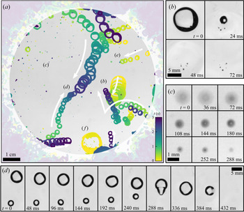
A relatively fast frame rate (83 Hz) is used to gain insight into the surface bubble dynamics and typical time scales. Figure 15 shows a sequence of 3 s of typical bubble activity at the surface of clean water (figure 15a), and associated singularized events (figure 15b–f). A primary observation is that only a small fraction of the emerging bubbles (about 10 out of 500 to 1000 per second) make their way into the region of interest. There, these are entrained towards the centre of the region at velocities up to 0.1 m s $^{-1}$ by the surface part of a large recirculation flow (figure 15d,e). The latter is itself driven by the bubbles rising in the bulk, with an upwards velocity of about 0.3 m s
 $^{-1}$.
(a) Three seconds of typical bubble activity at the surface of clean water, with 690 bubbles being produced per second in the bulk. The sequence is recorded at 10.4 Hz and stacked with the minimum value of each pixel over time, coloured with respect to time. White arrows indicate the general direction of motion for the nearest bubbles. The outer surfacing area is shaded. (b) A bubble bursting event, generating small bubbles from the retraction of the cap. Frames read from left to right, then top to bottom, separated by  ${\rm \Delta} t = 24$ ms. (c) A drop, initially out of focus, falls back on the bath and rebounds, losing mass;
 ${\rm \Delta} t= 36$ ms. (d) A merging event, rapidly followed by a burst;
 ${\rm \Delta} t = 48$ ms, rotated from (a). (e) A bubble emerging in the surfacing area and moving in the monitored region. (f) A bubble nearly 100 times as large as the injected individual volume.

The lifetime of surface bubbles in still clean water is known to be a quantity highly sensitive to the environment (surface contamination by airborne pollutants, water temperature, air humidity, etc.). As a result and even in the case of very careful experiments, it is broadly distributed, with values ranging from 0.1 to 10 s for centimetric bubbles (Zheng, Klemas & Hsu Reference Zheng, Klemas and Hsu1983; Poulain et al. Reference Poulain, Villermaux and Bourouiba2018). From a long time series, as the one presented in figure 15(a), we observe a similar variability, from bubbles newly merged that burst within a few tens of milliseconds (figure 15d, last four frames) to long-living bubbles that can travel around and cross the central region undisturbed (figure 15a,d). Indeed, this time scale  ${O}(0.1\text {--}1\ \text {s})$ compares well with the transport time of such bubbles across the central region (with diameter of around 0.1 m, to be divided by the typical velocity 0.1 m s
 $^{-1}$), allowing them to come into close proximity with other bubbles, and coalesce (figure 15d). With clean water, coalescence is inevitable: once two bubbles touch, they merge, with a coalescence time scale from contact to full shape recovery of about 0.1 s. The multiple and successive coalescence processes allow the formation of bubbles up to five times their initial size, with volumes that can be a hundred times the initial, injected volume
 $\langle V_b \rangle$ (figure 15b,f).
The bubbles eventually burst (figure 15b,d). On some occasions, bursting re-entrains submillimetric air bubbles, much smaller than the burst bubble, seen in figure 15(b). Bursting also generates droplets that may travel high and fall back, bounce onto the liquid surface and merge with the bath (figure 15c). Those drops, especially when they are close to the surface, are difficult to distinguish from the bubbles (figure 15a,c). As for the large remainder of the surfacing bubbles that do not reach the region of interest, they either move away from it, surfacing at the outer side of the rim, or burst before attaining it.
4.2. Raft regime in the presence of surfactant
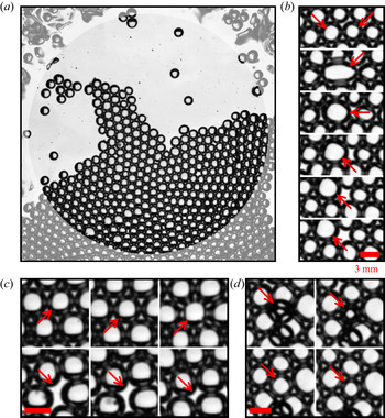
Figure 8(b) introduces a dense regime of surface bubbles, featuring a higher concentration of surfactant  $c$ (when compared to the case in figure 8a), non-coalescing bubbles and the formation of surface bubble rafts, or clusters. The clusters in figure 8(b) (or later in figure 17a) are made of almost single-sized bubbles, with diameter
 $\langle d_b \rangle$. At that particular time, the main cluster covers about a half of the region of interest, being rejoined by smaller clusters and individual bubbles moving around at the surface.
Figure 16 details 30 s of typical dynamic activity of the bubbles at the surface in this dense regime, by means of the bubble velocity distributions over time. Horizontal Cartesian components  $v_x$ and
 $v_y$ are shown in figure 16(a,b), and the velocity norm
 $v = (v_x^2+v_y^2)^{1/2}$ is plotted in figure 16(c) along with the bubble density
 $\rho _s$. Successive phases in the bubble behaviour at the surface can be distinguished. Bubbles sometimes move all as one, all having the same velocity, as is seen at times
 $t = 0\text {--}3$ s and
 $t = 12\text {--}15$ s in figure 16. Interestingly, this corresponds to a maximal density regime, the surface being entirely covered by bubbles arranged in a hexagonal two-dimensional packing: the surface bubble density is then
 $\rho _s = \rho _{hex} = 1/2\sqrt {3}\langle d_b \rangle ^2$, the density of perfectly aligned discs with constant diameter
 $\langle d_b \rangle$. Between such coordinated phases, bubbles burst and re-accumulate at the surface and the density
 $\rho _s$ fluctuates on time scales of order 1 to 5 s (figure 16c). The velocity distribution is then much broader, indicative of less coordinated motion of the bubbles at the surface.
Surface bubble horizontal velocity distributions  $n_s(v_s)$ as a function of time, illustrative of the raft regime with surfactants (
 $c = 92\ \mathrm {\mu }$M), at intermediate flow rate
 $q_v = 63$ cm
 $^3$ min
 $^{-1}$ (size in the bulk
 $\langle d_b \rangle = 3.6 \pm 0.4$ mm). Cartesian components (a)
 $v_x$ and (b)
 $v_y$, and (c) norm
 $v = (v_x^2 + v_y^2)^{1/2}$ of the velocity. The concentrations of velocities in narrow ranges (dark blue ridges, e.g.
 $t = 0\text {--}3, 12\text {--}15$ s) indicate a coordinated motion of all bubbles, alternating with less coordinated phases (broader histogram at given times, e.g.
 $t= 8\text {--}10\ {\rm s}$,
 $17\text {--}19$ s). (
 $c$, right-hand axis) Surface bubble density
 $\rho _s$. We indicate
 $\rho _{hex} = 1/2\sqrt {3}\langle d_b \rangle ^2$, the density of a two-dimensional hexagonal packing of discs with uniform diameter
 $\langle d_b \rangle$ (dashed line).

Figure 17(a) presents a typical cluster excerpted from the series in figure 16, and zooms in to identify events occurring for individual bubbles at faster time scales (10 to 100 ms; figure 17b–d). The sequences in figure 17(b,c) point to events similar to ones already observed in the dilute regime, though happening at a much slower rate: figure 17(b) shows the coalescence of two bubbles and figure 17(c) the bursting of a bubble. Both events leave a blank in the raft, which quickly reorganizes to resorb it. Figure 17(d) underlines the possibility of a three-dimensional organization of the bubbles at the surface: a bubble is initially trapped underneath the raft. However, it quickly emerges and makes its way among its neighbours, in the two-dimensional cluster. The reverse mechanism, i.e. the active trapping of bubbles by the cluster, from two- to three-dimensional organization, has not been observed: all trapped bubbles are caught underneath the raft while they try to emerge at the end of their rising, and then they drift away with the raft, staying below it until they ultimately surface within it.
(a) A surface bubble raft in the presence of surfactant, at intermediate flow rate ( $c = 92\ \mathrm {\mu }$M,
 $q_v = 63$ cm
 $^3$ min
 $^{-1}$). (b–d) Three typical events, each reading from left to right, then top to bottom. Consecutive frames are separated by
 ${\rm \Delta} t = 24$ ms; scale bars are 3 mm. (b) Coalescence of two bubbles (second frame). (c) A bubble bursts (third frame), leaving a blank in the raft, which eventually resorbs. (d) A bubble, initially trapped underneath the bubble raft, surfaces into the raft.

The previously described mechanisms, namely large-scale drifting, bubble bursting and merging, and occasional bubble trapping, are the ways the ensemble of bubbles spontaneously responds to the steady influx of non-coalescing and long-lasting bubbles. With the exception of the trapped bubbles, and despite high concentrations of SDS, under the experimental conditions presented in this paper no formation of a three-dimensional foam, one natural way to overcome the constant injection of bubbles in a bounded plane, was observed.
5. Surface bubble statistics
We now turn to a statistical description of the different regimes, over much longer time scales, having shown in figure 8 that the set-up is statistically stationary.
5.1. The case with clean water
When the water is clean, the coalescence of neighbouring bubbles is inevitable (Oolman & Blanch Reference Oolman and Blanch1986): bubbles at the surface therefore grow in size (figure 15b,d,f), preserving their total volume, until they burst. Figure 18 shows the surface bubble probability distribution function in terms of the volume  $V_s(d_s)$ (figure 18b), as well as the corresponding distributions
 $n_s(d_s)$ for the sizes measured at the surface and
 $n_b(d_b)$ in the bulk (figure 18a). Distributions
 $n_s$ are given per unit area, so that
 $\rho _s=\int n_s(d_s)\,\mathrm {d}d_s$ is the surface bubble density. The Gaussian distribution in the bulk, centred around the mean size
 $\langle d_b \rangle$ in the bulk, is also shown and matches the first peak of the surface size distribution (figure 18a), confirming that most of the bubbles have indeed the size of the injected bubbles.
Distributions, for clean water, of bubbles at the surface  $n_s$ (left-hand axis, black symbols) and in the bulk
 $n_b$ (right-hand axis, red) for a low flow rate
 $q_v = 25$ cm
 $^3$ min
 $^{-1}$. (a) Size distributions
 $n_s(d_s)$ and
 $n_b(d_b)$. The vertical dotted line indicates the bulk bubble mean size
 $\langle d_b \rangle$. (b) Volume distributions
 $n_s(V_s(d_s)/\langle V_b \rangle )$ and
 $n_b(V_b/\langle V_b \rangle )$, where volumes are normalized by the bulk bubble volume
 $\langle V_b \rangle = \pi \langle d_b^3 \rangle /6$. Vertical dotted lines are located at integer values of
 $\langle V_b \rangle$ and highlight corresponding peaks in the distribution
 $n_s(V_s/\langle V_b \rangle )$.

Surface bubble volumes  $V_s$ are normalized by the volume of the mean injected bubble
 $\langle V_b \rangle = \pi \langle d_b^3 \rangle /6$, with the first peak in the surface bubble volumes at
 $V_s = \langle V_b \rangle$ (figure 18b). The next peaks are located at
 $V_s/\langle V_b \rangle = 2, 3, 4, 5$, etc., and are the signature of the additivity of volumes during bubble merging events. The distribution of sizes and volumes is therefore extremely broad. This volume conservation, in addition to the air mass conservation at bubble merging, is a manifestation of air incompressibility under the experimental conditions. Pressure inside the bubbles is
 $p_{atm} + 4\gamma /R_{cap}$, with
 $p_{atm}$ the atmospheric pressure, typically
 $10^5$ Pa,
 $\gamma$ the air–water interfacial tension and
 $R_{cap}$ the bubble cap radius. For millimetric bubbles in clean water, the Laplace contribution
 $4\gamma /R_{cap} \sim 100$ Pa lies well below the atmospheric contribution, and the pressure drop due to the increase in
 $R_{cap}$ after bubble merging is negligible, hence the apparent volume conservation.
5.2. Surface size distribution in the presence of surfactants
The addition of surface-active material modifies the behaviour of bubbles in different ways, preventing the coalescence of bubbles and increasing their lifetime. Figure 19 shows surface bubble size distributions  $n_s(d_s)$ for various concentrations of surfactant SDS, and two different flow rates (
 $q_v = 31$ and 50 cm
 $^3$ min
 $^{-1}$). Along with the different distributions in figure 19(a,b), we present eight snapshots corresponding to each case, to help visualize the gradual changes at the surface.
Bubble size  $d_s$ distributions for different SDS concentrations
 $c$, below and above the coalescence threshold
 $c_0 \sim 10\ \mathrm {\mu }$M, and two flow rates: (a)
 $q_v = 31$ cm
 $^3$ min
 $^{-1}$ and (b)
 $q_v = 50$ cm
 $^3$ min
 $^{-1}$. Increasing
 $c$ above
 $c_0$ prevents coalescence and stabilizes bubbles, decreasing the size dispersion, and increasing the density around the bulk size
 $\langle d_b \rangle$, indicated in the vertical black dashed line. The column on the right shows still images from the respective series.

For clean water and small values of concentration ( $c \leq 1\ \mathrm {\mu }$M), the surface bubble size distribution presents peaks around the mean injection size
 $\langle d_b \rangle$ and slightly above (figure 19a,b, solid and dashed lines). This is the signature of the volume-conservative coalescence described in § 5.1. After a few numbers, the successive peaks overlap and contribute to a long, heavy tail, indicating that bubbles still coalesce, at all sizes. We resolve the statistics for bubbles with up to five times their injection diameter
 $\langle d_b \rangle$, which corresponds to a hundred times their injection volume
 $\langle V_b \rangle$. Although the heavy tail on the diameter distribution exhibits a reasonable agreement with an exponential distribution, we discuss in § 5 that the volume distribution is better interpreted by a power-law tail. We rationalize and discuss the argument in § 6.
For a high concentration value ( $c \geq 100\ \mathrm {\mu }$M), the distribution of
 $d_s$ is sharply peaked around the peak of injection size
 $\langle d_b \rangle$ (figure 19a,b, dotted lines). The surface distribution
 $n_s(d_s)$ is thus similar to the bulk distribution of sizes
 $n_b(d_b)$, since coalescence events are suppressed by surface-active contaminants.
An intermediate regime is distinguished for concentrations around  $c = 10\ \mathrm {\mu }$M. With a low flow rate
 $q_v = 30$ cm
 $^3$ min
 $^{-1}$, a second and a third peak at approximately
 $2^{1/3}\langle d_b \rangle$ and
 $3^{1/3}\langle d_b \rangle$ are still visible and indicate that surfacing bubbles keep merging (figure 19a, dash-dotted line). However, they do so in much smaller proportions, 10 to 100 times less, when compared to the value of the distribution
 $N_d(d_s)$ around the injection size
 $\langle d_b \rangle$. At the higher flow rate
 $q_v = 51$ cm
 $^3$ min
 $^{-1}$, the transition from a heavy-tailed distribution (coalescence regime) to the peaked distribution around the injection size
 $\langle d_b \rangle$ (non-coalescence regime) is more gradual (figure 19b, dash-dotted lines). In this case, bubbles still coalesce to populate larger sizes, in proportions similar to the case without surfactant. But even more bubbles stay around the injection size
 $\langle d_b \rangle$, hence narrowing the distribution around the major peak.
We note the production of bubbles with sizes much smaller than  $\langle d_b \rangle$. Figure 19(a,b) shows a large number of events around
 $d_s = 500\ \mathrm {\mu }$m, in the cases with
 $c \leq 1\ \mathrm {\mu }$M (solid and dashed lines; those small bubbles are not detected in the cases with a higher
 $c$, due to a difference in the bubble detection algorithm, but may be seen in the third- and second-to-last snapshots in figure 19). This peak aggregates indistinguishably: submillimetric bubbles surfacing from the bulk (see § 2.3.2), bubbles being formed at the collapse of a bursting bubble cavity, air pockets trapped under the retracting and collapsing bubble cap when bursting, as well as droplets falling back on the water surface after being ejected during a bubble bursting event.
Eventually, figure 19 highlights an extremely important result from a practical point of view. In the case of relatively clean water, where bubble coalescence is possible, the surface size distribution is much broader than the bulk size distribution of bubbles, so that surface bubble distributions should be considered when thinking of sea spray production.
5.3. Bubble surface fraction and clustering
Figures 8(c) and 8(e) reveal the major trend discussed in this article, that the bubble surface density  $\rho _s$ increases with an increased surfactant concentration
 $c$. Figure 19 then outlines that increasing
 $c$ also leads to a sharp decrease of the bubble variability around the mean injection size
 $\langle d_b \rangle$. However,
 $\rho _s = \int n_s(d_s)\,\mathrm {d}d_s$, the zeroth moment of the size distribution, does not incorporate any bubble size information, and we need to turn to its second moment:
 \begin{equation} \phi_s = \frac{\pi}{4}\int_{d_s} n_s(d_s) d_s^2\,\mathrm{d}d_s. \end{equation}
In the current representation,  $\phi _s$ is non-dimensional and, physically, is the surface area covered by the bubbles or the bubble surface fraction.
Figure 20 shows the evolution of the bubble surface fraction  $\phi _s$ as a function of the experimental control parameters for both surfactants SDS and Triton: air flow rate
 $q_v$ (figure 20a,c) and surfactant concentration
 $c$ (figure 20b,d). Figure 20(a,c) highlights the general increase of
 $\phi _s$ with the flow rate
 $q_v$, with colour encoding the surfactant concentration
 $c$. The trend is particularly clear with clean deionized water (open symbols), where an increase in the flow rate
 $q_v$ from 20 to 120 cm
 $^3$ min
 $^{-1}$ leads to a factor of 10 gained in the bubble surface fraction
 $\phi _s$, from
 $10^{-2}$ to
 $10^{-1}$. For equivalent flow rates, a smaller needle size leads to higher values of
 $\phi _s$ (figure 20a, symbol size), which is mediated by the greater number of bulk bubbles of small size generated at the needle tip, as shown in figure 6. With SDS, when increasing the surfactant concentration from 0.1
 $\mathrm {\mu }$M (figure 20a, yellow symbols) to 1 mM (red symbols),
 $\phi _s$ increases and quickly reaches the value
 $\phi _{hex} = \pi /2\sqrt {3}$. This upper bound is barely overcome, as it is the maximal value for
 $\phi _s$ for a perfectly hexagonal arrangement of monodisperse particles. Note that values higher than
 $\phi _{hex}$ in figure 20 are either an effect of compression of the bubbles assembled in rafts at the surface, or simply an experimental error (the raft dense detection method, as described in the Appendix, might lead to some slight, non-physical, overlap of bubbles on the plane; see e.g. figure 8b). This potential error remains in the global level of dispersion of our experimental data.
Bubble surface fraction  $\phi _s$ as a function of (a,c) the air flow rate per needle
 $q_v$ and (b,d) the surfactant concentration
 $c$ for surfactants (a,b) SDS and (c,d) Triton. Cases with deionized water are shown as open symbols. The horizontal dashed black line at
 $\phi _{hex} = \pi /2\sqrt {3}$ is the two-dimensional hexagonal arrangement of monodisperse hard discs. A variety of bubbling conditions are indicated by the different symbols: their sizes stand for different needle inner diameters (203 to 432
 $\mathrm {\mu }$m), squares and circles for different surface areas available to bubbles (full tank: 36 dm
 $^2$; and restricted area: 7 dm
 $^2$, respectively).

Figure 20(b,d) presents the same data for the bubble surface fraction  $\phi _s$, now as a function of the surfactant concentration
 $c$, with the colour encoding the air flow rate. The two regimes identified above are retrieved for both surfactants. At low levels of surfactant concentration, bubbles burst and coalesce quickly and bubbles have a small imprint on the surface:
 $\phi _s$ is low. Above a certain concentration (20
 $\mathrm {\mu }$M for SDS, 10
 $\mathrm {\mu }$M for Triton), the surface becomes saturated with single-sized, long-living bubbles and the upper limit
 $\phi _s = \phi _{hex}$ is reached. For even higher surfactant concentrations, bubbles will pile up in multiple layers, making any reliable measurements impossible in the present configuration.
Interestingly, the transition between the two regimes is continuous, even though it occurs on a limited range of concentration. It is especially visible from figure 20(b) (SDS) that the details of the bubble production (air flow rate, needle size, needle number, total surface area available to bubbles) have, in the explored range of parameters, a limited impact on the transition from clean to contaminated regimes. The precise behaviour of the bubbles in the transition from clean to contaminated regimes may finally depend on a variety of parameters. The surfactant itself, as seen when comparing figures 20(b) and 20(d), seems to have a primary role. The global trend for SDS, though blurred by variabilities in other parameters, is a smooth increase over two orders of magnitude. Conversely, for Triton there is a non-monotonic transition, increasing from the clean regime to concentrations around  $c \approx 0.6\ \mathrm {\mu }$M, then decreasing up to
 $c \approx 3\ \mathrm {\mu }$M, before rising again sharply to
 $\phi = \phi _{hex}$ at
 $c \approx 10\ \mathrm {\mu }$M. Among other parameters of lesser importance, the total area available to bubbles may influence the way bubbles emerge at the surface, and thus modify
 $\alpha$ in ways that may contribute to the scatter of data (figure 20b).
This non-trivial transition reaffirms the need for an accurate description of bubble behaviour at the surface, which we understand as a surface transfer function. As a last remark, we emphasize again that these variations all occur for low values of surfactant concentration, when compared to the CMC (respectively  $8.2$ mM and
 $220\ \mathrm {\mu }$M for SDS and Triton).
5.4. Order at the surface
The radial distribution function is another way of quantifying the level of order in the two-dimensional assembly of bubbles, and is exhibited in figure 21 for different concentrations of surfactant. It states, for a bubble individualized in the set, the likelihood of finding a neighbour at a distance  $\chi _s$ from its centre. A value of 1 at all distances means that there is no preferential separation distance, which is the case for the clean water – regardless of the meniscus interactions, which do not set any equilibrium distance. For high values of
 $c$, the structure of the hexagonal close packing appears, with well-defined peaks at distances
 $\chi _s/\langle d_b \rangle = 1, \sqrt {3}, 2, \sqrt {7}, 3$, etc. The experimental illustration by Bragg & Nye (Reference Bragg and Nye1947), exhibited here as a reference, was making the case of an atomic crystalline structure with a two-dimensional ‘perfect crystalline raft of bubbles’.
Radial distribution function for an increasing concentration of SDS, below and above the threshold for coalescence  $c \approx 6\ \mathrm {\mu }$M (solid lines). The dotted black line is computed from figure 4 of Bragg & Nye (Reference Bragg and Nye1947), which illustrates a ‘perfect crystalline raft of bubbles’ with diameter
 $\langle d_b \rangle = 0.3$ mm. The numbers are the exact locations of neighbours in a hexagonal close packing of hard discs with a diameter of 1.

6. A model for collective surface bubble statistics
We now develop a phenomenological model, with analytical foundations and a computational implementation. We aim at reproducing and rationalizing the surface statistics described in § 5 with minimal physical ingredients. The steps included in the model formulation are rooted in the physical observations made in §§ 3, 4 and 5, which we recall here:
(i) bubbles are introduced at the surface at a constant rate;
(ii) bubbles are introduced with a unique size;
(iii) depending on the surface contamination, bubbles can either grow in size by coalescence or cluster in rafts;
(iv) coalescence events preserve the total volume of the bubbles involved; and
(v) bubbles have a finite lifetime and finally disappear by bursting.
The model formulation and its numerical implementation are described in § 6.1. The outcomes of the cellular automaton are then compared with experimental data in § 6.2, in both clean and contaminated regimes. We also discuss the role of the numerical parameters, and how they identify with their experimental counterparts. The scope of the model is finally discussed in § 6.3.
6.1. Discrete model and cellular automaton implementation
A discrete model is developed that features the physical arguments enumerated above. We consider an ensemble of bubbles with discrete diameters  $d_k\ (k \geq 1)$, scattered on a plane with surface area
 $\mathcal {A}$. Bubbles with size
 $d_k$ have a density
 $n_k$ (i.e. number of bubbles with size
 $d_k$ divided by
 $\mathcal {A}$), evolving according to the three mechanisms identified previously: bubble production, coalescence and bursting. Bubble merging, in particular, is the only way (under a production of monodisperse bubbles) for bubbles to grow in size and populate higher ranks
 $k > 1$. When they coalesce, bubbles
 $i$ preserve their total volume
 $\sum _i d_i^3$, so that the ensemble contains only bubbles with sizes
 $d_k = k^{1/3} d_1$.
In this representation the first moments of the distribution of sizes  $n_k(d_k)$ yield important physical content. The moment of order zero is the bubble surface density:
 \begin{equation} \rho_s = \sum_{k \geq 1} n_k. \end{equation}
The first moment is the mean bubble size:
 \begin{equation} \langle d_s \rangle = \frac{1}{\rho_s}\sum_{k \geq 1} n_k d_k. \end{equation}
The second moment is directly proportional to the bubble surface fraction  $\phi _s$:
 \begin{equation} \langle d_s^2 \rangle = \frac{1}{\rho_s}\sum_{k \geq 1} n_k d_k^2 = \frac{4}{\pi} \frac{\phi_s}{\rho_s}. \end{equation}
Note eventually that the motion of bubbles, specifically their mutual attraction via meniscus interactions, is not modelled here, as we are interested in much longer, integrated and statistically independent time scales.
6.1.1. Numerical implementation
The numerical implementation of the model is a cellular automaton. The ensemble of bubbles (sizes  $d_k$, densities
 $n_k$) undergoes, at each iteration in the simulation, the following steps, where we define the parameters of the simulation.
(i) New bubbles with size
$d_1$ are introduced in the set with production rate $p_1$ per unit area (per iteration). This rate is chosen to be a random variable normally distributed, with a dispersion of typically ${\pm }20$% around its mean.(ii) Bubbles are removed from the set according to their age
$s$ (i.e. time spent in the simulation): old bubbles are more likely to burst than young ones. The bubble lifetime distribution is modelled by a Weibull distribution with shape parameter 4/3, following (3.9) in Lhuissier & Villermaux (Reference Lhuissier and Villermaux2012). The cumulative distribution function, evaluated at bubble age $s$, is naturally the bursting probability for each bubble, at each simulation step. The distribution is scaled by $\tau$, the mean bubble lifetime, given in simulation steps.(iii) The bubbles of the set are scattered randomly, with a uniform spatial distribution, over the total available surface area
$\mathcal {A}$.(iv) Bubble pairs whose edge-to-edge distance lies under a certain criterion
$\ell$ may merge into a new bubble, according to a pair-coalescence probability $m$. If merging, they add up their volumes. Bubble pairs are considered by increasing distances (closest merge first), with no iterative handling of triplets of overlapping bubbles, or more. In the event of overlapping bubbles, and at low enough bubble surface fraction, potential anomalies are assumed to resorb at the next iteration, when bubbles are shuffled again. The age of the merged bubble is set to $s = 0$.(v) Bubbles are passed on to the next iteration with their age
$s$ increased by one iteration $s+1$.


The merging scheme (iv) is based on the assumption that two bubbles at the surface of clean water, when close enough, will attract and finally merge with probability  $m$ (
 $m =1$ in clean water, and decreases with the surface contamination; Oolman & Blanch Reference Oolman and Blanch1986; Vella & Mahadevan Reference Vella and Mahadevan2005). Note that the probability
 $m$ is taken independent of the bubble size. The threshold distance,
 $\ell$ in the computational model, is the typical length over which bubbles start or cease to attract each other. Physically, it represents the bubble meniscus typical size and scales as the capillary length of the liquid
 $\ell _c$. By setting and holding
 $\ell = d_1$, we set the bubble unit size
 $d_1$ around the capillary size, a situation similar to experiments (see § 2).
Figure 22 illustrates the outcome of a typical simulation in a coalescence regime ( $m = 1$), by plotting the bubble density
 $\rho _s$ and mean size
 $\langle d_s \rangle$ as a function of successive iterations
 $s$. The domain size is
 , with
 $p_1\mathcal {A} = 9 \pm 2$ bubbles introduced per iteration, and the bubble mean lifetime is
 $\tau = 10$ iterations. Figure 22(a,c) zooms in the first instants of the simulation, run for a variety of initial conditions (1 to 60 bubbles, all with size
 $d_1$). As seen for both the surface density
 $\rho _s$ and bubble mean size
 $\langle d_s \rangle$, the bubble system reaches a stationary state within a relatively small number of iterations, typically 10 to 20. Figure 22(b,d) follows a single simulation for a much larger number of iterations (up to 2000, or 200 bubble mean lifetimes), and helps appreciate the system stationarity in the long run. A final comparison of the simulation at short times, with multiple runs (figure 22a) and of a single run over long times (figure 22b), makes the case for an equality, in a statistical sense, of ensemble and time averages.
Evolution of (a,b) the bubble density  $\rho _s$ (black lines) and (c,d) the mean diameter
 $\langle d_s \rangle /d_1$ (red lines) in the course of a simulation run. At each iteration,
 $p_1\mathcal {A} = 9 \pm 2$ bubbles are introduced on a square with side
 $\sqrt {\mathcal {A}} = 30 d_1$. Bubble mean lifetime is
 $\tau = 10$ iterations so that the total run is
 $200\tau$. (a,c) Zoom on the first 50 iterations, showing the transient, from different initializations (0 to 60 bubbles with size
 $d_1$, thin lines) to a stationary state. (b,d) View of a single simulation over a larger number of iterations.

6.2. Role of the model controlling parameters and comparison with experiments
A quantitative comparison of the model with the surface statistics requires one to inform the simulation production rate  $p_1$, pair-coalescence probability
 $m$ and bubble mean lifetime
 $\tau$ with characteristic scales inferred from experiments, respectively the surface bubble production rate
 $p_s$ (§ 2.3), merging rate
 $q_m$ and bursting rate
 $q_b$ (§ 3), which we do in the following paragraphs.
6.2.1. Coalescence regime
The coalescence regime (clean deionized water; see § 5.1) is a peculiar case where bubbles systematically merge when close enough, and they burst at a fixed rate. Therefore, the pair-coalescence probability is set to  $m=1$ and the bubble mean lifetime to some value large enough for bubbles not to burst immediately after they are introduced or merging (typically around 10 iterations, at least).
The only parameter left to vary is then the bubble production rate. Experimentally, bubbles are introduced in the bulk at various flow rates  $q_v$, which amount to various bubbling rates
 $p_s$ into the imaged region (surface area
 $\mathcal {A}$). The bubble production rate
 $p_s$ is made non-dimensional by expressing the available area in units of
 $\langle d_s \rangle$ and time in units of the surface bubble mean lifetime
 $\langle \tau _s \rangle$. By (2.2) and (2.3), this is
 \begin{equation} \tilde{p} (\text{exp.}) = \alpha \frac{\pi \langle d_b \rangle^2}{4\mathcal{A}} p_b \langle \tau_s \rangle = 1.086 \alpha \frac{N_{needles}}{\mathcal{A}} q_v^{3/5} g^{1/5} \langle \tau_s \rangle. \end{equation}
We consider in the following a fixed value of  $\alpha = 1/3$, thought of as a generic order of magnitude, but acknowledge that its precise value might slightly change with the flow rate or the total area available to bubbles, due to complex raft dynamics which goes beyond the scope of a strictly statistical description (bubble and raft drifting, surface flows, etc.). The mean bubble lifetime is estimated as that of a single bubble bursting
 $\langle \tau _s \rangle \approx 1$ s at 20
 $^\circ$C (Poulain & Bourouiba Reference Poulain and Bourouiba2019). This value is consistent with the bursting rates
 $q_b$ measured in the bubble raft decay at low concentrations of surfactant (§ 3.3). Finally
 $\tilde {p}(\text {exp.})$ is calculated and takes values, in the clean water cases, in the range 0.01–0.1 (i.e. 0.01 to 0.1 bubbles introduced in the system per mean lifetime).
The corresponding expression for  $\tilde {p}$ in the model is straightforward and reads
 \begin{equation} \tilde{p} (\text{num.}) = p_1 \tau. \end{equation}
Figure 23 compares experiments and simulations in the regime of clean water ( $m=1$). Figure 23(a) shows experimental distributions of bubble volumes at the surface of clean water, under three air flow rates (i.e. bubble production rates), in physical units (lines). The surface densities are relatively low and a long power-law tail emerges from the logarithmically scaled graph:
 $n_s (V_s) \propto V_s^r$, with an exponent
 $r \simeq -3/2$. Note that we do not have a theoretical argument for this robust power-law distribution. Also note that for increasing flow rates, the amplitude of the peak at
 $V_s = \langle V_b \rangle$ decreases, indicating a lower bubbling rate as predicted by (2.2).
Experimental and simulated surface bubble volume distributions in the coalescence regime. (a) Experimental distributions (lines) for three different flow rates  $q_v = 25, 50, 100$ cm
 $^{3}$ min
 $^{-1}$ in clean water (respectively
 $\tilde {p} = 0.04, 0.06, 0.1$). Vertical dashed lines indicate the average bulk volume
 $\langle V_b \rangle$ in each case. (b) Lines duplicate the experimental distributions in (a), volumes being normalized by
 $\langle V_b \rangle$ (
 $x$ axis) and counts by the surface area in units of
 $\langle d_b^2 \rangle$ (
 $y$ axis). The markers are for three simulated distributions, with respective production rates
 $\tilde {p} = 0.04, 0.06, 0.1$ and lie on top of the experimental distributions.

In figure 23(b), experimental bubble volumes are normalized by their respective injected bulk volume  $\langle V_b \rangle$, and their numbers by the monitored area now expressed in units of
 $\pi \langle d_b^2 \rangle /4$, leading to the normalized surface size distribution
 $n_s (x = V_s / \langle V_b\rangle )$. They are directly compared with three simulated distributions, run for the same values of
 $\tilde {p} = [0.04, 0.06, 0.1]$ (symbols; mean lifetime is
 $\tau =16$ iterations, domain size
 $\sqrt {\mathcal {A}} = 100 d_1$ and increasing production rate
 $p_1 = [2.5, 3.7, 6.2] \times 10^{-3}$). We observe strong similarities between the experimental and simulated distributions for both the power-law tail of the distributions, with the same exponent
 $r = -3/2$, and the evolution of their amplitude, with an increased bubble production at
 $V_s = \langle V_b \rangle$ (
 $V_k/V_1$ in the automaton model) leading to more bubbles
 $n_s(V_s)$ at all volumes
 $V_s$. Given the assumptions of the automaton model, the agreement is remarkable. The remaining discrepancies are attributed to the uncertainties on
 $\alpha$ and
 $\langle \tau _s \rangle$ when computing
 $\tilde {p}(\text {exp.})$ (6.4).
In the coalescence regime, the transfer function from the bulk to the surface transforms narrow, monodisperse bubble distributions into broad, power-law-tailed distributions. Our parameterization for this transfer function highlights the role of merging events. It captures successfully, owing to the identification of the non-dimensional bubbling rate  $\tilde {p}$, the main features of the experimental observations: orders of magnitude, distribution shape and trends.
6.2.2. Merging and bursting in the cellular automaton
As shown in § 3, the addition of surfactants in water has two distinct effects: on the ability of the bubbles to coalesce and on their individual lifetime. In the automaton simulation, both effects are entirely decoupled: the merging ability is modelled by the individual pair-coalescence probability  $m$, whereas the lifetime is specified by the shape of the lifetime distribution and its scaling
 $\tau$. Figure 24 shows surface bubble volume distributions from simulations for various merging probabilities
 $m$ (figure 24a) and mean lifetimes
 $\tau$ (figure 24b), under a fixed bubble production rate
 $\tilde {p} = 0.1$. In figure 24(a), the pair-coalescence probability
 $m$ is decreased from 1 (the merging of eligible bubbles is systematic) to
 $10^{-3}$, with a fixed mean lifetime
 $\tau = 32$ iterations. The respective distributions narrow gradually around the bubble injection volume
 $V_1$, reproducing faithfully the main feature of the transition from clean to contaminated regimes.
Simulated surface bubble volume distributions in the partial coalescence regime with a fixed bubble production rate  $\tilde {p} = 0.1$. (a) The pair-coalescence probability is decreased from
 $m = 1$ to
 $10^{-3}$, with a fixed mean lifetime
 $\tau =20$. (b) The mean lifetime is increased from
 $\tau = 10$ to 80, with a fixed pair-coalescence probability
 $m = 0.1$.

In figure 24(b), the mean lifetime  $\tau$ is increased from 16 to 128 iterations, for a fixed pair-coalescence probability
 $m = 0.1$. The change in
 $\tau$, at fixed
 $\tilde {p}$, has no observable effect on the shape of the distribution. It has, however, a moderate effect on the scaling of the distribution: longer lifetimes
 $\tau$, because bubbles spend on average more time in the simulation and are therefore more likely to undergo a successful merging event, lead to fewer bubbles populating all sizes, i.e. a decrease in the overall distribution levels. It is worth recalling here that
 $\tau$ is also involved in the calculation of
 $\tilde {p} = p_1 \tau$ (6.5), which is kept constant. An increase in
 $\tau$ while considering a constant bubble production
 $p_1$, instead of a constant
 $\tilde {p}$, will result more intuitively in an increase of the overall bubble numbers.
With the two parameters  $m$ and
 $\tau$, the simulations are able to reproduce the phenomenology described in the presence of surfactant in figure 19 in a notable way. On the one hand, the distribution shape is controlled by
 $m$, from very broad at high value of
 $m$ to more and more narrow as the merging efficiency is decreased to zero. On the other hand, the lifetime
 $\tau$ acts directly on the amplitude of the distribution, which increases with increasing lifetime.
We now perform a more detailed and quantitative comparison of experiments and simulations, using the dynamical measurements of merging and bursting rates made in § 3 to tune and match  $m$ and
 $\tau$ with their physical counterparts.
6.2.3. Partial coalescence regime
Experimentally, variations in the partial coalescence regime are achieved by modifying the sole concentration of surfactant  $c$, whereas the numerical model can vary with both the pair-coalescence probability
 $m$ and the mean lifetime
 $\tau$ independently. Recalling findings from § 3, below a transition concentration
 $c_*$, coalescence dominates the life of an assembly of bubbles. Merging then depends on the bubble surface fraction
 $\phi _s$ (bubbles attract and merge when they are close enough), and so does bursting. Above
 $c_*$, coalescence vanishes quickly with increasing surfactant concentration, in a progression that we consider geometric for simplicity, and similar for both the merging rate
 $q_m$ and pair-coalescence probability
 $m$:
 $m \sim q_m \sim c^{-\beta }$, with
 $\beta = 1.5$.
The evolution for the bubble mean lifetime  $\langle \tau _s \rangle$ is less critically dependent on the coalescence transition, as
 $\langle \tau _s \rangle$ globally increases with the concentration of surfactant (Lhuissier & Villermaux Reference Lhuissier and Villermaux2012; Modini et al. Reference Modini, Russell, Deane and Stokes2013; Champougny et al. Reference Champougny, Roché, Drenckhan and Rio2016). When coalescence becomes negligible, i.e. for high surfactant concentrations
 $c \gg c_*$,
 $\langle \tau _s \rangle$ is well approximated by the global decay time
 $\tau _r$ of the raft, as measured in § 3 (figure 11):
 $\tau _r \approx 1/q_b \sim \langle \tau _s \rangle$. In particular, the global raft decay time
 $\tau _r$ was observed to plateau across the transition, before increasing again. We represent schematically these trends for the merging rate
 $q_m$ and bubble mean lifetime
 $\langle \tau _s \rangle$ in figure 25(a), as a basis for the choices of parameters.
Comparison of experimental and simulated surface bubble distributions in the partial coalescence regime. (a) Schematic trends for merging rate  $q_m$ (green solid line) and bubble lifetime
 $\langle \tau _s \rangle$ (red dashed line; see also § 3), associated with numerical parameters
 $m$ and
 $\tau$, respectively. Four concentrations of surfactant are selected below (
 $c_0 = 0$), around (
 $c_1\simeq c_*, c_2 = 2c_1$) and above the transition (
 $c_3 = 10c_1 \gg c_*$) to compare with numerics. (b) Bubble volume distributions in the statistically stationary experiment for increasing concentrations
 $c$ of SDS (thin lines, reproduced from figure 19 in a non-dimensional way), and from the cellular automaton (thick lines and symbols). Simulations are run with a constant bubble production
 $p_1 = 0.01 \pm 25\,\%$ on a domain with size
 $\sqrt {\mathcal {A}} = 40 d_1$. Numerical curves are shifted vertically for clarity. The variations and selection of
 $m$ and
 $\tau$ follow the trends in (a). Their values are summarized in the table (c), and discussed in the text.

A case-by-case comparison between experimental and simulated bubble distributions is plotted in figure 25(b), from a clean water case ( $c_0 =0$), across the coalescence transition (
 $c_1 \approx c_*$ and
 $c_2 = 2c_1$) and asymptotically further into the partial to non-coalescence regime (
 $c_3 = 10c_1 \gg c_*$). The experimental values and trends for the bubble merging rate
 $q_m$ and lifetime
 $\langle \tau _s \rangle$, though not exactly matching the definition of their numerical counterparts, inform the choice of parameters
 $m$ and
 $\tau$ in the following way.
(i) The first case is taken in clean water
$c_0 = 0\ \mathrm {\mu }$M: $m_0 =1$, as discussed in § 6.2.1. It helps us match the production rate $\tilde {p}_0 = 0.1$, and the initial bubble lifetime $\tau _0 = 10$ iterations.(ii) Next, the surfactant (SDS) concentration is increased to
$c_1=10\ \mathrm {\mu }$M, i.e. around the transition concentration $c_*$. The merging probability is decreased to $m_1 = 0.05$, and the mean lifetime is increased to $\tau _1 = 20$ iterations, matching the sharp reduction in the bubble merging ability and the increase in bubble lifetime.(iii) In the third case, the SDS concentration is increased further to
$c_2 = 20\ \mathrm {\mu }$M, above the transition and into the plateau of the raft decay time. Lifetime $\tau _2 = 20$ is thus kept constant. The coalescence probability is decreased according to the geometrical decay $m_2 = m_1 (c_1/c_2)^\beta \approx 0.02$.(iv) In the last case,
$c_3 = 10 c_1 = 100\ \mathrm {\mu }$M, and thus $m_3 = m_1 /10^\beta \approx 0.001$. Having reached the end of the plateau, the bubble mean lifetime is increased further to $\tau _3 = 40$ iterations.


As seen in figure 25(b), and given the somewhat coarse approach, the agreement is good. The shapes of the numerical distributions, with the parameters  $m$ and
 $\tau$ varied according to an inferred evolution with respect to a unique surface contamination control parameter (the surfactant concentration
 $c$ in the experiments), narrow down gradually around the injection volume
 $V_1$, in a way similar to that in the experiments. As a last remark, we do not fully capture the strong increase in the amplitude of the experimental distributions as
 $c$ is increased. This is attributed to the fact that bubbles can overcome the meniscus length and stay in close contact in the experiment (see e.g. figure 8b), which does not happen in the simulation without modifying the numerical meniscus distance
 $\ell$.
6.3. Discussion of the transfer function from bulk to surface controlling parameters
We demonstrate with figures 23, 24 and 25 that the parameterization of the bubble transfer function from the bulk to the surface depends on a limited number of variables, which we identify. The merging of bubbles – when coalescence is likely to happen – is essential for building broad distributions from monodisperse bubbles, and depends directly on the pair-coalescence probability  $m$. Preventing coalescence (i.e. decreasing
 $m$) therefore narrows the surface distribution around the bubble bulk size, but fails to explain the large increase in absolute number of bubbles at the surface, as observed experimentally. This increase is first attributed to the bubble production rate, which has a direct influence on the surface density, as is shown in figure 23(b).
However, when the production rate  $p_1$ is kept constant, the bubble mean lifetime
 $\tau$ is the second parameter that influences the bubble density. We recall that
 $\tau$ scales the global bubble lifetime distribution, where old bubbles are more likely to burst than young ones. With an increased mean bubble lifetime
 $\tau$, and the number of bubbles being introduced at each iteration being the same, bubbles thus last longer before bursting, on average, which de facto increases the population at the surface. Experimentally, an increased concentration of surfactant modifies the two parameters
 $\tau$ and
 $m$, where the numerical model allows their independent study.
Conversely, and as a final comment, a small mean lifetime will not only interfere with the bubble production, but also with the coalescence ‘dynamics’, which has no intrinsic time scale other than the simulation step  $s$. A markedly small
 $\tau$ would thus burst bubbles before they are even able to merge, keeping the surface bubble distribution narrow around the injected size, and to low density value.
7. Conclusion
This article demonstrates that, in the overall process of spray production by bursting bubbles, coming for instance from breaking wave events, knowledge of the bulk bubble distribution is not enough to predict the surface bubble distribution, and hence shall certainly fail to predict alone the spray properties accurately (number, sizes). We rejoin a cohort of authors in claiming that surface contamination controls the behaviour of the bubbles at the surface (Garrett Reference Garrett1967; Modini et al. Reference Modini, Russell, Deane and Stokes2013; Prather et al. Reference Prather2013), and draw a precise experimental picture of its role in large assemblies, or clusters, rafts or even whitecaps, of bubbles. With no doubt, the detailed description of this intermediate stage between bulk bubble production and spray formation, the bulk–surface transfer function, will prove useful in the finer characterization of the spray drops themselves, and identification of the (collective) mechanisms at play.
Depending on the surface contamination, presently modelled by surfactants SDS and Triton, a nearly monodisperse assembly of millimetric air bubbles produced identically in the bulk of a water bath behave in very different ways at the surface. Two asymptotic regimes are identified by means of experiments measuring the dynamics and the statistics of such assemblies, and confirmed by a cellular automaton model based on a handful of physical arguments. Their distinctive features are
(i) a clean surface regime, with short-lived and coalescing bubbles, exhibiting low surface density and fraction, despite large bubbles resulting from the merging of up to a hundred bubbles of the initial size; and
(ii) a contaminated surface regime, with long-lasting and non-coalescing bubbles, where the surface bubble distribution tends towards the bulk bubble distribution for high levels of contamination, and surface density, surface fraction and order tend towards a hexagonal network of bubbles, the arrangement which maximizes packing in two dimensions.
The transition between these two regimes appears to depend on the surfactant itself, in a non-monotonic, non-trivial fashion. The identification and use of the global merging and bursting rates  $q_m$ and
 $q_b$ is a first step towards the parameterization of the bulk–surface transfer function, envisioned here from a dynamical point of view. It temporarily allows one to avoid the need for a physicochemical analysis of the water interface, as could be the case when performing the experiment with liquids of partially known composition (e.g. seawater scooped out of the open ocean). However, a precise link to the physicochemistry of the interface will be required in the pursued ambition of a complete parameterization of the bulk–surface transfer function.
The case of seawater, with a more complex chemical and biological composition, certainly lies between those regimes. Figure 26 shows a visual comparison of three rafts of bubbles, produced under similar laboratory conditions, respectively in the clean regime, with artificial seawater and in the contaminated regime. In seawater, the presence of bubbles with multiple sizes is a clear indication that bubbles merge and burst at the same time: it is a last demonstration of the need for a comprehensive bulk–surface transfer function.
Three snapshots of rafts in (a) deionized water and SDS ( $c = 8\ \mathrm {\mu }$M), (b) artificial seawater and (c) deionized water and SDS (
 $c = 256\ \mathrm {\mu }$M) under similar room conditions and bubble production. They illustrate where seawater stands with respect to merging and bursting: in a partial coalescence regime, between the asymptotic clean and fully contaminated regimes.

The discrete formulation we derive for two-dimensional assemblies of bubbles gives physical grounds to a numerical and statistical implementation of the bulk–surface transfer function. It takes the form of a cellular automaton, which is informed by dynamical quantities directly inferred from experiments. Despite the simplicity of the numerical model, distribution shapes, orders of magnitude and trends with respect to the surface contamination and bubble production rates are retrieved and compared successfully with the experiments. The identification and matching of numerical and experimental parameters are successful, supporting the need for the development of a more general framework, embracing all contaminations, and eventually linking the bulk bubble production mechanisms to the spray production in raft regimes.
In future studies, the statistically stationary bubble plume set-up will offer possible variations on a greater number of parameters, allowing in particular the refinement of the link with the water physicochemistry: the needle size(s), down to 200  $\mathrm {\mu }$m in diameter; the needle number, virtually any number between 1 and 48; the water temperature, from room temperature to multiple tens of degrees Celsius; the water salinity, from clean water to sea conditions; the surface contamination, with any soluble surfactant.
Acknowledgements
We thank D. Ruth and R. Alert for fruitful discussions, and D. Yancopoulos for participation in preliminary experiments, through the High Meadows Environmental Institute summer of learning programme. We thank the three anonymous reviewers whose comments helped improve the quality of the manuscript.
Funding
This work was supported by the National Science Foundation (Physical Oceanography) under grant no. 1849762 to L.D.; the Cooperative Institute for Earth System Modeling between Princeton and GFDL NOAA; and the Princeton Catalysis Initiative and the High Meadows Environmental Institute.
Declaration of interests
The authors report no conflict of interest.
Appendix. Surface bubble detection
The detection of isolated bubbles at the surface of water does not present technical difficulties. However, when bubbles assemble in rafts and touch each other, the only way to detect them unambiguously is to use their inner contour. Figure 27 presents the mode of operation. Figure 27(a) shows surface bubbles in a cluster, along with the detection of their inner edges. We then carefully select, from data acquired under the same conditions of lighting, a set of isolated bubbles of various sizes, such as the one exhibited in figure 27(b), for which both inner ( $d_m$) and outer (
 $d_s$) diameters are measured. We finally use a linear fit to calibrate, in the dense regime, the actual size of the bubbles
 $d_s$, given the measured inner diameter
 $d_m$. Figure 27(c) shows an example of such a plot of
 $d_s$ as a function of
 $d_m$, and the associated best linear fit.
Bubble detection and calibration in the raft regime. (a) Bubble inner edge detection in a cluster. (b) Detection of the inner (red) and outer (white) edges of an isolated bubble. (c) Linear calibration from the inner diameter  $d_m$ to the bubble diameter
 $d_s$.