

The percentage of children with elevated blood lead levels [in Flint, MI] increased after water source change, particularly in socioeconomically disadvantaged neighborhoods. Water is a growing source of childhood lead exposure because of aging infrastructure. (Hanna-Attisha et al., Reference Hanna-Attisha, LaChance, Sadler and Champney Schnepp2016)
1. Introduction
Research documenting that disadvantaged groups of society are disproportionately exposed to environmental pollution is abundant (e.g., Mohai et al., Reference Mohai, Pellow and Roberts2009; Laurent, Reference Laurent2011; Banzhaf, Reference Banzhaf2012; Banzhaf et al., Reference Banzhaf, Ma and Timmins2019). The causes of such “toxic inequalities” are numerous and often intertwined. Two prominent factors contributing to environmental injustice are regulatory failure and intergenerational transmission of poverty.Footnote 1 They pose challenges for policymakers who seek to alleviate environmental inequalities while respecting people’s preferences for health and safety (Fleurbaey et al., Reference Fleurbaey, Luchini, Muller and Schokkaert2013; Adler, Reference Adler2016; Sheriff & Maguire, Reference Sheriff and Maguire2020). One particularly startling example is inequalities caused by exposure to neurotoxic substances – lead in drinking water or mercury in the vicinity of coal-fired power plants are salient examples – that impair the cognitive development of children. The impacts are often irreversible, affecting exposed individuals throughout their lives (Grönqvist et al., Reference Grönqvist, Nilsson and Robling2020), and are predominantly borne by children who grow up in disadvantaged neighborhoods (Currie, Reference Currie2011).
Exposure to neurotoxic substances often coincides with and amplifies existing social inequalities. For instance, Aizer et al. (Reference Aizer, Currie, Simon and Vivier2018) find that disadvantaged children in Rhode Island are more likely to be exposed to lead, which may be one of the reasons for the observed disparities in math and reading test scores among students from different socioeconomic backgrounds. In the long run, toxic inequalities create a vicious circle in which the cognitive ability of parents impacts their disposable income and, through that, determines in which neighborhood their children are raised (see Figure 1). Children’s cognitive ability becomes the joint outcome of genetic and environmental factors, which in turn affects their future earnings and, through that, their own location choices. Thus, social inequalities tend to be passed on from generation to generation (Bowles & Gintis, Reference Bowles and Gintis2002).Footnote 2
Pyramid of toxic inequalities (adapted from Banzhaf and McCormick (Reference Banzhaf, McCormick and Banzhaf2012)).

Figure 1. Long description
The diagram is structured as a large triangle with a central variable.
Core and Vertices:
* At the center is Parents’ I Q.
* The top vertex is Child’s income.
* The bottom-left vertex is Child’s I Q.
* The bottom-right vertex is Neighborhood.
Numbered Pathways:
* Pathway 1: An arrow points from Parents’ I Q to Child’s I Q, labeled Genetic factors.
* Pathway 2: An arrow points from Parents’ I Q to Neighborhood, labeled Parents’ location choice.
* Pathway 3: An arrow points from Neighborhood to Child’s I Q, labeled Environmental factors.
* Pathway 4: A vertical line with an upward arrow points from Parents’ I Q to Child’s income, labeled Behavioral factors.
* Pathway 5: An arrow points from Child’s I Q up the left side of the triangle toward Child’s income, labeled Labor market outcome.
* Pathway 6: An arrow points from Child’s income down the right side of the triangle toward Neighborhood, labeled Child’s location choice.
A legend on the right side of the diagram explicitly lists the definitions for numbers 1 through 6.
The traditional economics approach to neighborhood location choices has been based on hedonic pricing, which holds that non-market goods and services are bundles of attributes that are fully internalized in the housing market (Bishop et al., Reference Bishop, Kuminoff, Banzhaf, Boyle, von Gravenitz, Pope, Smith and Timmins2020). All else being equal, the presence of toxic substances in a neighborhood should lower housing prices in that area. However, in the context of environmental pollution, we see at least two problems with the hedonic approach. First, pollution will not be adequately reflected in the housing prices that prevail before the public becomes aware of the threat. Second, even if the potential for exposure to toxic substances is (partially) internalized by the housing market (Currie et al., Reference Currie, Davis, Greenstone and Walker2015), prices do not reflect the intergenerational effects identified above unless home buyers are explicitly considering them.
Since housing prices are unlikely to accurately reflect exposure to neurotoxic substances and other invisible pollutants, economists have come up with alternative approaches to assess the benefits of cleanup projects and pollution prevention policies. The standard practice is to measure the pollution-induced harm in terms of IQ loss and convert it to the expected lifetime earnings loss faced by affected individuals (Grosse et al., Reference Grosse, Matte, Schwartz and Jackson2002). However, this approach fails to capture distributional aspects of environmental pollution and ignores that the income elasticity of demand for the provision of environmental goods – or the avoidance of environmental bads – is commonly found to be substantially smaller than unity (Baumgärtner et al., Reference Baumgärtner, Drupp, Meya, Munz and Quaas2017; Drupp et al., Reference Drupp, Meya, Baumgärtner and Quaas2018). In other words, standard benefit–cost analysis (BCA) is silent about inequalities in exposure to harmful substances, and these “toxic inequalities” are further compounded by income inequalities.
In theory, the marginal willingness-to-pay (WTP) to avoid the loss of one IQ point should be proportional to the expected income gain and any other utility derived from avoiding this loss. This implies that the burden of neurotoxicity as measured by unweighted WTP is lower if poorer people bear the brunt of pollution. Accordingly, if one is solely interested in efficiency, then programs aimed at restoring the environmental status of poorer neighborhoods are comparatively less desirable than those targeted at better-off neighborhoods (Harberger, Reference Harberger1978). Such a strong focus on efficiency is at odds with fairness considerations widely recognized by BCA scholars (Adler, Reference Adler2016; Fleurbaey & Abi-Rafeh, Reference Fleurbaey and Abi-Rafeh2016; Banzhaf, Reference Banzhaf2023; Fleurbaey & Hammitt, Reference Fleurbaey and Hammitt2024). Moreover, the efficiency argument is only valid under the assumption that costless lump-sum transfers are feasible (Johansson-Stenman, Reference Johansson-Stenman2005), and it depends on the numéraire chosen for the analysis (Hammitt, Reference Hammitt2021). Lastly, unweighted BCA has also been criticized for violating democratic principles as it favors some people systematically over others (Nyborg, Reference Nyborg2014).
This paper presents a non-welfarist approach to analyzing unequal exposure to toxic pollutants that incorporates fairness considerations while respecting individual preferences. To fix ideas, we introduce the tale of Janusville – a fictional town where the poorer half of the population live on the B side and the richer half reside on the A side. Income in Janusville is approximately lognormally distributed. Intelligence would be normally distributed (with a mean IQ of 100 points and a standard deviation of 15 points), if it were not for the contamination of drinking water that causes children growing up on the B side to have two IQ points less than they would have otherwise. As suggested by Figure 1, the labor market outcome of these children will be determined by both their intelligence and the support they receive from their parents. Together these factors imply that the prospective income of children growing up on the B side of Janusville is lower than that of children growing up on the A side.
Let us assume that the town council gathers to decide whether they should invest in a cleanup project benefiting children on the B side only or spend the money on an educational program to help children across town to grapple with life. Both programs are thought to provide the same aggregate IQ gain for future generations and entail the same costs.Footnote 3 The council debates which program is better. This is a thorny question as it relates to how the distribution of intelligence will eventually affect aggregate income, and what that means. Taking efficiency as the core criterion, the town should strive for the IQ distribution that maximizes aggregate income. However, it seems ethical to demand the town council consider fairness aspects in its evaluation.
In the remainder of the paper, we seek to advise the town council of Janusville on the program choice considering different ethical principles for dealing with distributive justice. Our approach is based on the concept of equivalent income, which we define as the hypothetical income that makes an individual indifferent between their current well-being endowment (in terms of consumption, health, social status, work-life balance, etc.) and a well-being endowment that fixes all but the individual’s income to specific reference levels (Fleurbaey, Reference Fleurbaey, Adler and Fleurbaey2016). Equivalent income is an attractive concept for making interpersonal comparisons because it accounts for differences in resource endowments while respecting individual preferences.
Unlike previous applications of the equivalent income concept in the health domain (e.g., Fleurbaey et al., Reference Fleurbaey, Luchini, Muller and Schokkaert2013; Samson et al., Reference Samson, Schokkaert, Thébaut, Dormont, Fleurbaey, Luchini and Van de Voorde2018), we explicitly consider the interdependence of health and wealth (Fuchs, Reference Fuchs2004; Deaton, Reference Deaton2008). This is particularly relevant for the relationship between IQ and income as more intelligent individuals tend to earn more than less intelligent ones. In Section 2, we set out the theoretical background and present a welfare model that accounts for the feedback effect between IQ and income. Section 3 introduces equivalent income as a non-welfarist measure of individual preferences and shows how it may be used to obtain theoretically sound welfare weights that can be employed in applied BCA. In Section 4, we apply the concept to the question of program choice faced by the town council of Janusville, contrast it to the results obtained with standard BCA, and highlight the normative challenges with each approach. Section 5 concludes.
2. Theoretical background
We start with a simple model in the spirit of Fleurbaey et al. (Reference Fleurbaey, Luchini, Muller and Schokkaert2013) to address unequal exposure to neurotoxic substances in Janusville.Footnote
4 The situation of individual
$ i=1,\dots, n $
 is described by the tuple
$ \left({y}_i\left({g}_i\right),{g}_i\right) $
 , where
$ {g}_i $
 denotes
$ i $
 ’s intelligence (typically measured in IQ) and
$ {y}_i\left({g}_i\right) $
 is their prospective income, which itself is a function of intelligence. Building on Bergson (Reference Bergson1938) and Samuelson (Reference Samuelson1947), our model evaluates the vectors
$ \left({y}_1\left({g}_1\right),{g}_1\right),\dots, \left({y}_n\left({g}_n\right),{g}_n\right) $
 in terms of a real-valued social welfare function (SWF):
$ W\left({u}_1\left({y}_1\left({g}_1\right),{g}_1\right),\dots, {u}_n\left({y}_n\left({g}_n\right),{g}_n\right)\right) $
 , where
$ {u}_i $
 expresses individual
$ i $
 ’s preferences.
$ W $
 is thus a numerical representation of society’s preference ordering, which we assume to respect the Pareto principle. This implies that
$ W $
 assigns the same value to those states of the world in which everyone is equally well-off.
Since we attempt to model the situation in Janusville, we focus on the welfare effect of a marginal gain in intelligence
$ {dg}_i $
 but abstract from other factors that affect prospective income
$ {y}_i $
 . Taking the full differential of
$ W $
 , we define an infinitesimal change to the initial situation as follows:

The right-hand side of Equation (1) can be further decomposed. Using customary notation,
$ {\beta}_i\equiv \frac{\partial W}{\partial {u}_i}\frac{{\partial u}_i}{{\partial y}_i} $
 accounts for the marginal welfare that society derives from individual
$ i $
 being marginally better off. The terms in square brackets represent
$ i $
 ’s willingness-to-pay (WTP) for obtaining the marginal gain in intelligence
$ {dg}_i $
 . Specifically,
$ \frac{\partial {y}_i}{\partial {g}_i}{dg}_i $
 is the expected change in prospective income due to the gain in intelligence, while
$ \frac{{\partial u}_i}{\partial {g}_i}\frac{{\partial y}_i}{\partial {u}_i}{dg}_i $
 captures the gain in utility (converted into a money equivalent) and thus represents the hedonic value of intelligence.
With this in mind, we may rewrite Equation (1) as a weighted sum of individual WTPs:

As discussed in detail by Fleurbaey et al. (Reference Fleurbaey, Luchini, Muller and Schokkaert2013), Equation (2) incorporates both empirical and ethical considerations.
$ {\mathrm{WTP}}_i $
 may be derived from market observations or elicited by stated preference methods, while
$ {\beta}_i $
 is a parameter that measures how a gain in
$ i $
 ’s prospective income should be compared with similar gains accruing to other individuals (Boadway, Reference Boadway2006). By definition,
$ {\beta}_i $
 consists of (i) an ethical component,
$ \frac{\partial W}{\partial {u}_i} $
 , that reflects how much society values an extra unit of utility accruing to person
$ i $
 ; and (ii) an empirical component,
$ \frac{\partial {u}_i}{{\partial y}_i} $
 , that reflects
$ i $
 ’s marginal utility from income. Based on common fairness arguments, society should give more weight to those individuals whose starting point is less favorable, for example, because of unequal exposure to pollution.
Three broad arguments have been made against the use of distributional weights in BCA (Boadway, Reference Boadway2006; Adler, Reference Adler2016; Acland & Greenberg, Reference Acland and Greenberg2023): (i) the focus of BCA should be on efficiency; (ii) according to the Kaldor–Hicks compensation, principle income could, at least in theory, be distributed in a Pareto-efficient way; and (iii) everyone can expect to be better off in the long-run, since eventually positive net payoffs from various policy changes will even out among individuals. In a first-best world, the efficiency argument has merit because government can redistribute income without affecting labor supply choices (Boadway & Keen, Reference Boadway and Keen1993; Kaplow, Reference Kaplow1998). We will briefly discuss the first-best solution before turning to the more realistic second best in which authorities have limited power over the tax schedule. Typically, local authorities cannot levy and redistribute taxes independently, but they may still seek to address equity concerns in public projects while respecting citizens’ preferences.Footnote 5
2.1. First-best solution
To establish a benchmark, we first apply the logic of standard BCA, which ignores distributional concerns entirely and evaluates policies solely based on aggregate, unweighted WTP (Banzhaf, Reference Banzhaf2023). In keeping with this logic, the first-best solution refers to a situation in which government can redistribute income without constraints. In other words, any post-transfer income distribution
$ \left({y}_1,\dots, {y}_n\right) $
 that preserves the total sum of income is feasible (Adler, Reference Adler2016). Ignoring differences in the marginal utility of income across individuals, and under the maintained assumptions of costless redistribution and a fully monetized welfare metric, the socially optimal solution is to maximize total income
$ Y={\sum}_i{y}_i $
 and redistribute it so that
$ {\beta}_i=\beta $
 for all
$ i $
 . This allows us to normalize
$ \beta $
 to unity without loss of generality.
Under these assumptions, a policy that seeks to reduce detrimental impacts on population-level intelligence should maximize aggregate WTP for the attainable increase in IQ:

where
$ {x}_i $
 refers to the absolute IQ gain that individual
$ i $
 can expect from a policy whose cost is
$ C $
 ; accordingly,
$ X $
 is the achievable population increment in IQ (i.e., the total IQ points gained across the population). In order to be meaningful, the allocation of
$ X $
 needs to come from a feasible set (i.e., we exclude all allocations that would result in some individuals having an extraordinary IQ).
Equation (3) suggests that government should prioritize those with the highest WTP for IQ changes and the terms in brackets are decisive for the choice of policy. If we presume that average income increases with IQ and the marginal rate of substitution between intelligence and income is also increasing in income, then
$ {\mathrm{WTP}}_i $
 is higher for wealthier people. Applying this result to Janusville suggests that an educational program targeting both sides of town (or just the A side) would be preferable to a cleanup project that benefits only the B side. This is because the additional gains in prospective income from the educational program could, in theory, be re-distributed to the less well-off. This argument, widely known as the potential Pareto test, was devised by Kaldor and Hicks precisely to circumvent distributional issues in BCA (Banzhaf, Reference Banzhaf2023).
2.2. Second-best solution
Readers may object to this advice on ethical grounds since the first-best solution disregards inequalities in exposure to neurotoxic substances. Moreover, the assumption of perfect redistribution is unrealistic for most real-world applications. Instead, we now consider that Janusville has no discretionary powers to levy and redistribute taxes and must finance public projects from a given budget. This assumption allows us to study the implications of limited redistribution without explicitly modeling labor-leisure responses (see Johansson-Stenman et al., Reference Johansson-Stenman, Carlsson and Daruvala2002). However, it also breaks the first-best equivalence and motivates the search for a second-best solution.
Given the constraint on income transfers, the town should maximize the weighted sum of individual WTPs:

where the notation is the same as in Equation (3); accordingly,
$ {\beta}_i\left[\frac{\partial {y}_i}{\partial {g}_i}+\frac{{\partial u}_i}{\partial {g}_i}\frac{{\partial y}_i}{\partial {u}_i}\right] $
 is
$ i $
 ’s weighted WTP for an IQ increment of exactly one point. In contrast to the first best,
$ {\beta}_i $
 depends on individual
$ i $
 ’s initial endowment of income and IQ. The big question is now how the weights should differ between individuals with different initial endowments. Any answer to this question involves ethical considerations regarding how society ranks gains in utility to different individuals and empirical considerations related to how individuals’ utility changes when their income or intelligence increases.
Since the weight
$ {\beta}_i $
 given to individual
$ i $
 can be broken down into
$ \frac{\partial W}{\partial {u}_i} $
 and
$ \frac{\partial {u}_i}{\partial_{y_i}} $
 , we can study how different ethical considerations affect the weights. Whereas utilitarians assume
$ \frac{\partial^2W}{\partial {u}_i^2}=0 $
 and thus apply the same weight to all utility changes, prioritarians maintain that more weight be given to those in less favorable circumstances, that is,
$ \frac{\partial^2W}{\partial {u}_i^2}<0 $
 .Footnote
6 Regardless of one’s ethical view, less weight should thus be given to a person with a higher initial endowment, and vice versa. The weights affect how BCA accounts for the terms in brackets in Equation (4), where the first term captures the expected change in income from a one-point gain in IQ. Because labor economists find that gains in income increase with concurrent IQ (e.g., Lin et al., Reference Lin, Lutter and Ruhm2018), we assume that this term is marginally increasing in
$ {g}_i $
 . The second term describes the marginal rate of substitution between IQ and income and may hence be seen as the WTP for a one-point gain in IQ.
To implement this second best, the town council needs advice on how to (i) construct meaningful welfare weights and (ii) estimate the income demand elasticity for IQ points. Distributional weights are typically larger for poorer individuals, reflecting diminishing welfare gains to society from improving people’s well-being. Yet, in absolute terms, wealthier individuals may be willing to pay more for health-related goods than poorer ones. This is reflected by Equation (4), where the two terms in brackets go in opposite directions as wealth increases. This implies that optimal program choice is primarily an empirical problem.
3. Distributional weights based on equivalent income
While Section 2 provided pragmatic solutions for program choice under different constraints, they both hinge on the weights assigned to individual WTPs. In this section, we discuss how these weights can be calibrated without making interpersonal comparisons of subjective well-being. To start with, suppose that interpersonal comparisons of subjective well-being were meaningful, and that marginal changes in subjective utility due to IQ changes could be readily measured. As Adler (Reference Adler, Adler and Norheim2022) discussed, these assumptions can be combined in a prioritarian SWF with an Atkinson transformation function that displays constant elasticity of substitution in utilities:

so that
$ {\beta}_i=\frac{\partial W}{{\partial y}_i}=\frac{{\partial u}_i}{{\partial y}_i}{u}_i{\left({y}_i\left({g}_i\right),{g}_i\right)}^{-\rho } $
 can be interpreted as a distributional weight that captures society’s aversion to inequality governed by the parameter
$ \rho $
 .Footnote
7 However, because this weight is based on interpersonal utility comparisons, it raises both practical and ethical concerns. It is simply unclear how subjective utility could be meaningfully compared between individuals.
One approach to addressing this issue is to assume that all individuals derive the same utility from income. This can be modeled by a constant elasticity function so that
$ {u}_i\left({y}_i\right)=\frac{{y_i}^{1-\varepsilon }}{1-\varepsilon } $
 , with
$ \varepsilon $
 being a constant coefficient of relative risk aversion (CRRA). Inserting the CRRA utility function into Equation (5) yields after some algebra:

with
$ \sigma =\varepsilon +\rho -\rho \varepsilon $
 (see Nurmi & Ahtiainen, Reference Nurmi and Ahtiainen2018). Accordingly, the distributional weight attached to individual
$ i $
 ’s income becomes
$ {\beta}_i={y}_i^{-\sigma } $
 , where the parameter
$ \sigma $
 combines diminishing marginal utility of income (as expressed by the relative risk aversion of individuals) with society’s relative inequality aversion. As noted by Kaplow (Reference Kaplow2010), the SWF given by Equation (6) may be interpreted as (i) a utilitarian welfare function with constant relative risk aversion, (ii) an egalitarian SWF with risk-neutral individuals or (iii) a combination of such preferences.Footnote
8
The weights implied by Equation (6) avoid interpersonal comparisons, but they also ignore other resources that the individual is endowed with, such as their baseline IQ. To capture differences in resource endowments, we assume that for every individual
$ i $
 there exists a compensating variation
$ {z}_i $
 such that
$ \left({y}_i\left({g}_i\right),{g}_i\right)\sim \left(\left({y}^{\prime}\left({g}^{\prime}\right)-{z}_i\right),{g}^{\prime}\right) $
 , where
$ {g}_i $
 and
$ {y}_i\left({g}_i\right) $
 are
$ i $
 ’s IQ and prospective income, respectively,
$ {g}^{\prime } $
 is a chosen reference level of IQ, and
$ {y}^{\prime}\left({g}^{\prime}\right) $
 is the after-tax income corresponding to that reference level.Footnote
9 In other words, individual
$ i $
 is willing to pay (or receive) the compensating variation
$ {z}_i={\int}_{g_i}^{g^{\prime }}\left[\frac{\partial {y}_i}{\partial {g}_i}+\frac{{\partial u}_i}{\partial {g}_i}\frac{{\partial y}_i}{\partial {u}_i}\right] dg $
 , where the first term in brackets captures the change in expected income when moving from the current IQ to the reference IQ. Below, we will denote this income change by
$ {\Delta y}_i\left({g}_i\to {g}^{\prime}\right) $
 . The second term in brackets corresponds to the hedonic value of intelligence, which we will denote by
$ {\mathrm{WTP}}_i\left({g}_i\to g^{\prime }|{y}_i\right) $
 .Footnote
10
There is a crucial difference between our setup and that of Fleurbaey et al. (Reference Fleurbaey, Luchini, Muller and Schokkaert2013). Namely,
$ {z}_i $
 captures both the direct effect of IQ on well-being and the feedback effect that IQ has on well-being via increased consumption potential (Fuchs, Reference Fuchs2004; Deaton, Reference Deaton2008). It allows us to formally define individual
$ i $
 ’s equivalent income as follows:

In the special case where
$ \frac{{\partial u}_i}{\partial {g}_i}\frac{{\partial y}_i}{\partial {u}_i}=0 $
 , the compensating variation simplifies to
$ {z}_i={y}^{\prime}\left({g}^{\prime}\right)-{y}_i\left({g}_i\right) $
 and the corresponding equivalent income becomes
$ {y}_i^{\ast}\left({y}_i\left({g}_i\right),{g}_i,{y}^{\prime },g^{\prime}\right)={y}_i\left({g}_i\right) $
 .Footnote
11 In other words, the inverse of the prospective income distribution is used to determine the distributional weights (Nurmi & Ahtiainen, Reference Nurmi and Ahtiainen2018).
Up to this point, we have defined the compensating variation
$ {z}_i $
 in terms of individuals’ marginal rates of substitution between income and intelligence. In this sense, the construction remained consistent with a welfarist perspective. Now, we impose additional structure by assuming a common relationship between income and the hedonic value of intelligence across individuals. As Fleurbaey et al. (Reference Fleurbaey, Luchini, Muller and Schokkaert2013) discuss in detail, with this assumption,
$ {y}_i^{\ast } $
 is not a welfarist measure anymore since it does not measure subjective utility, even though it satisfies the Pareto principle. To appreciate this point, consider two individuals who have the same income and IQ but value their resource endowment differently. In a welfarist framework like the one given by Equation (5), their different preferences would justify weighing these two individuals differently. Under the equivalent-income approach, however, both individuals are assigned the same equivalent income. Therefore, we can rewrite Equation (5) as
$ W\left({y}_1^{\ast },\dots, {y}_n^{\ast}\right). $

Upon inserting into Equation (7), the welfare change due to a change in population intelligence becomes:

This welfare change consists again of two factors – individual
$ i $
 ’s total benefit of a specified gain in intelligence,
$ \left[\frac{\partial {y}_i}{\partial {g}_i}+\frac{\partial {y}_i^{\ast }}{\partial {g}_i}\frac{\partial {y}_i}{\partial {y}_i^{\ast }}\right]{dg}_i $
 , and the corresponding weight
$ {\beta}_i=\frac{\partial W}{\partial {y}_i^{\ast }}\frac{\partial {y}_i^{\ast }}{\partial {y}_i} $
 , which indicates how society values this specific gain in comparison with the gains accruing to other individuals. Importantly, when using the equivalent-income approach, the weight assigned to each individual is a combination of ethical considerations captured by society’s valuation of equivalent income, that is,
$ \frac{\partial W}{\partial {y}_i^{\ast }} $
 , and empirical facts reflected by the expected change in equivalent income from a change actual income, that is,
$ \frac{\partial {y}_i^{\ast }}{\partial {y}_i} $
 .
Using the chain rule, we can break down Equation (8) further and rewrite the distributional weight as
$ {\beta}_i=\frac{\partial W}{\partial {u}_i}\frac{\partial {u}_i}{\partial {y}_i^{\ast }}\frac{\partial {y}_i^{\ast }}{\partial {y}_i} $
 . This decomposition makes clear that the weight captures three elements: society’s valuation of an individual’s utility, the curvature of individual utility in equivalent income, and the way changes in actual income translate into changes in equivalent income. If one takes the stance that intelligence per se is not part of an individual’s resource endowment and has only instrumental value in obtaining a larger income, then
$ \frac{\partial {y}_i^{\ast }}{\partial {y}_i}=1 $
 and thus
$ {y}_i^{\ast}\left({y}_i\left({g}_i\right),{g}_i\right)={y}_i\left({g}_i\right) $
 . Similarly to the steps in Equations (5) and (6), one obtains an Atkinson SWF function where the applicable weight boils down to
$ {\beta}_i={y}_i^{-\sigma } $
 .Footnote
12
Conversely, if intelligence is considered to be more than just a means to an end, the welfare weight becomes
$ {\beta}_i=\frac{\partial {y}_i^{\ast }}{\partial {y}_i}{\left[{y}_i^{\ast}\left({y}_i\left({g}_i\right),{g}_i\right)\right]}^{-\sigma } $
 , where
$ {y}_i^{\ast}\left({y}_i\left({g}_i\right),{g}_i\right)={y}_i\left({g}_i\right)-{\mathrm{WTP}}_i\left({g}_i\to g^{\prime }|{y}_i\right) $
 and
$ \frac{\partial {y}_i^{\ast }}{\partial {y}_i}=1-\frac{\partial {\mathrm{WTP}}_i\left({g}_i\to {g}^{\prime }|{y}_i\right)}{\partial {y}_i} $
 . In words, the welfare weight now reflects the individual’s valuation of intelligence captured by their WTP; the income dependence of this valuation through the mapping from actual income into equivalent income; and society’s distributive preferences over equivalent income expressed through the inequality aversion parameter
$ \sigma $
 . Note that also in this case the parameter
$ \sigma $
 captures both the diminishing marginal utility of income and social aversion to inequality.
To assess the interplay of these dimensions, we can rewrite
$ \frac{\partial {y}_i^{\ast }}{\partial {y}_i} $
 in terms of income elasticity of WTP. Define
$ {\eta}_i=\frac{y_i}{{\mathrm{WTP}}_i}\frac{\partial {\mathrm{WTP}}_i}{\partial {y}_i\;} $
 , then
$ \frac{\partial {y}_i^{\ast }}{\partial {y}_i}=1-{\eta}_i\frac{{\mathrm{WTP}}_i}{y_i} $
 . This expression is convenient as it allows us to distinguish three cases (Nurmi & Ahtiainen, Reference Nurmi and Ahtiainen2018): (i) if
$ \eta =1 $
 , then
$ \frac{\partial {y}^{\ast }}{\partial y} $
 is constant; (ii) if
$ \eta >1 $
 , then
$ \frac{\partial {y}^{\ast }}{\partial y} $
 falls with income; and (iii) if
$ \eta <1 $
 , then
$ \frac{\partial {y}^{\ast }}{\partial y} $
 rises with income. Assuming constant income elasticity means the factor
$ \frac{\partial {y}_i^{\ast }}{\partial {y}_i} $
 assigns relatively more weight to the poor (rich), whenever benefits are distributed progressively (regressively). When the income elasticity exceeds one, benefits are disproportionately valued by the rich, and the equivalent-income mapping further tilts the weights in favor of the poor. Conversely, when the income elasticity is below one, the mapping partially offsets the prioritarian tilt. Intuitively, when the non-income attribute is valued disproportionately more by poorer individuals, less additional reweighting toward the poor is required. Conversely, when richer individuals value the same attribute disproportionately more, stronger reweighting is warranted. Importantly, this adjustment does not reflect an ethical judgment but corrects for the income dependence of monetary valuation. Distributive preferences remain solely governed by the inequality aversion parameter
$ \sigma $
 .
4. Application
We now return to the challenge of advising the town council of Janusville and apply the framework developed above to evaluate the different policy options laid out in the introduction section. To facilitate this exercise, we need to make assumptions about the relationship between childhood IQ and future earnings. Fortunately, the impact of childhood IQ on future earnings has been widely studied (Lin et al., Reference Lin, Lutter and Ruhm2018). While existing studies differ with regard to outcome age, measure of income, extent to which non-cognitive factors were accounted for and the inclusion of other control variables, they all find a strong link between IQ and future earnings. For example, Cunha and Heckman (Reference Cunha and Heckman2016) find a convex relationship between productivity and both genetic and acquired cognitive abilities, implying that people with higher cognitive abilities are disproportionately rewarded by the labor market.Footnote 13
The direct change in utility from a gain in IQ expressed in monetary terms – that is, the hedonic value of a higher IQ – is less studied, since it cannot be readily inferred from market observations. The most relevant research we are aware of is a recent survey study by Mourato et al. (Reference Mourato, Atkinson, Dussaux, Sotis, Georgiou and Contu2023) in which 13,200 respondents from 11 OECD countries were asked to state their WTP for avoiding a specific IQ point loss in their children. Importantly, respondents were explicitly instructed not to focus on future income of their offspring but rather on how well their children would do in school. Mourato and her co-authors found that the WTP per IQ point increased with income, but not proportionately. In other words, IQ appeared to be a necessity rather than a normal good.
4.1. Janusville
We draw on these empirical findings to simulate the population of Janusville. Our simulation seeks to account for the causal relationships that influence a child’s labor market outcome as displayed by Figure 1. The starting point of our simulation is parental IQ and income, which together determine on which side of town a child will grow up. Neighborhood choices affect a child’s prospects because children living on the B side will be exposed to neurotoxic substances, while children living on the A side will not. Parental IQ also impacts a child’s IQ, which we capture by imposing a positive correlation between IQ and parents’ income. Eventually, a child’s IQ will determine their lifetime earnings via labor market outcomes.
We capture these relationships through 1,000 draws from a multivariate normal distribution with partial correlations between parents’ income, children’s IQ and expected lifetime earnings. We then use parental income as a sorting variable so that the poorer half of the population lives on the B side of Janusville and the richer half on the A side. Because parental income is positively correlated with both children’s IQ and expected lifetime earnings in the simulated distribution, this sorting induces systematic differences across neighborhoods not only in income but also in cognitive endowments. As a result, the B side is disadvantaged both in terms of income and IQ already prior to the pollution shock, capturing intergenerational persistence in social inequality.
For simplicity, we assume that each child growing up on the B side will lose two IQ points compared to a world in which no toxic inequalities existed. Consistent with findings by Lin et al. (Reference Lin, Lutter and Ruhm2018), we assume a reduction of two IQ points will reduce the lifetime earnings of these children by about 3%. Based on this setup, we derive the IQ and expected lifetime earning distributions shown in Figure 2, with a mean IQ of 94.4 on the B side and of 103.8 on the A side, respectively. Normalized to average lifetime earnings, income has a mean of 0.81 on the B side and 1.19 on the A side, respectively. The assumed correlation between parents’ income and their offspring’s IQ offspring is
$ \rho $
 = 0.3, which is broadly consistent with findings in the intelligence literature (e.g., Von Stumm & Plomin, Reference Von Stumm and Plomin2015).
Initial IQ and income distributions on both sides of Janusville.

Figure 2. Long description
A two-panel density plot with a legend on the far right. The legend identifies A side as pink and B side as teal.
Left Panel: I Q distribution.
The horizontal x-axis ranges from 50 to 150. The vertical y-axis represents Density from 0.00 to 0.05. Two bell-shaped curves overlap. The teal curve for B side peaks earlier at an I Q of approximately 95 with a density of 0.027. The pink curve for A side peaks later at an I Q of approximately 105 with a density of 0.027.
Right Panel: Income distribution.
The horizontal x-axis ranges from 0 to 150. The vertical y-axis represents Density from 0.00 to 0.05. Both curves are right-skewed. The teal curve for B side is narrower and taller, peaking sharply at an income of approximately 15 with a density of 0.043. The pink curve for A side is broader, peaking at an income of approximately 20 with a lower density of 0.030, and maintains a thicker tail as income increases toward 100.
4.2. Distributional weights in practice
Implementing the equivalent income weights introduced in Section 3 requires knowledge of the equivalent income for each individual, which is determined by the program choice as well as by the choice of the inequality aversion parameter
$ \sigma . $
 While future lifetime earnings are calibrated to empirical data in our simulation,
$ \sigma $
 is a policy parameter. There is a stream of literature discussing plausible values of
$ \sigma $
 based on both empirical findings (Dasgupta, Reference Dasgupta1998; Johansson-Stenman et al., Reference Johansson-Stenman, Carlsson and Daruvala2002) and ethical considerations (Anthoff et al., Reference Anthoff, Hepburn and Tol2009; Hallegatte et al., Reference Hallegatte, Vogt-Schilb, Bangalore and Rozenberg2016). Most studies suggest values of
$ \sigma $
 between 0.5 and 2 but recommend conducting a sensitivity analysis. Below, we explore values of
$ \sigma $
 between 0 and 3, noting that these extremes may be ethically less desirable.
To calculate the individual weight
$ {\beta}_i $
 , we normalize the equivalent income
$ {y}_i^{\ast } $
 . Typically, this is done by dividing through a specific reference income. While this normalization has neither an effect on the relative weights nor on the eventual choice of program, it does affect the aggregate scaling of a unit increase in monetized welfare. We, therefore, set the reference income equal to the minimum lifetime earnings in the simulated population so that the weight given to the worst-off individual equals unity. Figure 3 shows how the chosen inequality aversion parameter affects the relative weights. Note that with increasing inequality aversion, the weights become ever more sensitive to income.
Contour plot for different values of income and inequality aversion.

Figure 3. Long description
The x-axis represents Normalized income ranging from 0.0 to 1.0. The y-axis represents Individual weights ranging from 0.0 to 1.0. The plot contains seven shaded regions separated by curved contour lines, each labeled with a sigma value representing inequality aversion.
* At the top right, a dark blue region is bounded by a horizontal line at y equals 1.0 and a curve labeled sigma equals 0.
* Moving downward, the regions become progressively lighter shades of blue.
* The curve for sigma equals 0.1 shows a slight downward slope from left to right.
* As sigma increases to 0.25, 0.5, and 1.0, the curves exhibit increasingly sharp asymptotic behavior, curving steeply upward toward the y-axis as normalized income approaches zero.
* At the bottom left, the curves for sigma equals 2.0 and sigma equals 3.0 are compressed near the x-axis, indicating that weights drop rapidly to near zero for all but the lowest income levels.
4.3. Results of the simulation
Our simulations explore two distinct scenarios: redistribution of program benefits is possible (first best), and redistribution of benefits is not possible (second best).Footnote
14 For comparing the optimal solutions under each of these scenarios, we consider programs of continuous nature so that the attainable increase in aggregate IQ points can be distributed across the population in many ways. In reality, programs are not continuous but discrete proposals. This limits the choice problem to few policy options. We, therefore, modify the solutions obtained in Section 2 to a discrete choice among competing projects. Concretely, consider
$ j=1,\dots, m $
 mutually exclusive programs. Then, the first-best solution is given by:

while the second-best solution is attained by:

We apply Equations (
9
a) and (9
b
) to two discrete programs that are expected to result in the same aggregate gain in IQ points. Program
$ \boldsymbol{A} $
 is an educational project that seeks to benefit all children in Janusville and is expected to result in a one IQ point increase for every child. Program
$ \boldsymbol{B} $
 is a cleanup project that seeks to restore the counterfactual IQ distribution on the B side of town by eliminating inequalities in exposure to neurotoxic substances for future generations. Based on findings by Lin et al. (Reference Lin, Lutter and Ruhm2018), we assume that each IQ point gained will increase a child’s lifetime earnings by 1.45%. For simulating the hedonic value of intelligence, we rely on the results of Mourato et al. (Reference Mourato, Atkinson, Dussaux, Sotis, Georgiou and Contu2023). Specifically, we model WTP based on their estimates of (i) the income elasticity of WTP (
$ \hat{\eta}=0.4 $
 ), and (ii) their mean WTP per IQ point, which corresponds to approximately 1% of a person’s income. By solving the first-order linear differential equation that results from assumption (i), we obtain a WTP estimate for every individual in the population while respecting the initial condition of assumption (ii).
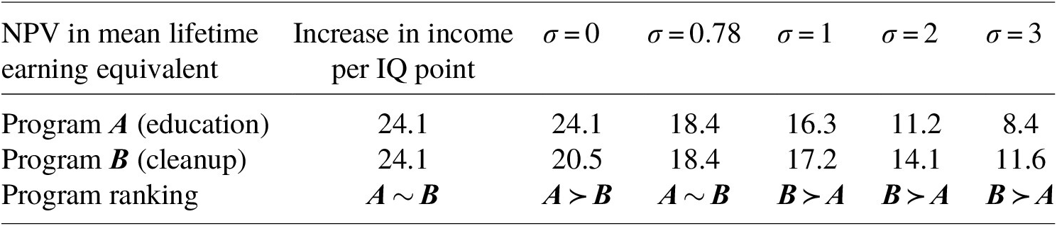
Table 1 summarizes the results of our simulation. The unweighted net present value (NPV) of the cleanup project (program
$ \boldsymbol{A} $
 ) is 20.5 average lifetime earning equivalents, whereas the unweighted NPV of the educational project (program
$ \boldsymbol{B} $
 ) amounts to 24.1 average lifetime earning equivalents.Footnote
15 This difference is brought about by lower income expectations on the B side of town. Thus, from a pure efficiency view, program
$ \boldsymbol{A} $
 should be chosen. However, if equity considerations are considered, program
$ \boldsymbol{B} $
 is preferred for any inequality aversion parameter
$ \sigma >0.78 $
 and the margins become larger the more inequality averse the decision maker is. As discussed above, the literature on inequality aversion supports values of
$ \sigma > $
 1. In our context, this may be further justified by the fact that exposure to pollutants is often caused by negligence, which advocates for inequality aversion being considered in BCA, since living in a polluted area may no longer be an economic choice but the consequence of knowing better.
Results of the simulation

Table 1. Long description
The table consists of seven columns and four rows.
Header Row: The first column is labeled N P V in mean lifetime earning equivalent. The second column is Increase in income per I Q point. The remaining five columns are labeled with the symbol sigma followed by values: sigma = 0, sigma = 0.78, sigma = 1, sigma = 2, and sigma = 3.
Row 1 (Program A education): Values are 24.1 for Increase in income per I Q point, 24.1 for sigma = 0, 18.4 for sigma = 0.78, 16.3 for sigma = 1, 11.2 for sigma = 2, and 8.4 for sigma = 3.
Row 2 (Program B cleanup): Values are 24.1 for Increase in income per I Q point, 20.5 for sigma = 0, 18.4 for sigma = 0.78, 17.2 for sigma = 1, 14.1 for sigma = 2, and 11.6 for sigma = 3.
Row 3 (Program ranking): This row uses mathematical symbols to compare the programs. For Increase in income per I Q point, A is similar to B. For sigma = 0, A is preferred over B. For sigma = 0.78, A is similar to B. For sigma = 1, sigma = 2, and sigma = 3, B is preferred over A.
The results in Table 1 reflect both the direct and indirect effects of a change in IQ on WTP. If one instead considers that intelligence is not in and of itself a source of individual well-being, then the weight for
$ \sigma =1 $
 becomes
$ {\beta}_i=\frac{\overline{y}}{y_i}, $
 and the corresponding weighted change in welfare is given by
$ {\mathrm{WTP}}_i^{\ast }=\frac{\overline{y}}{y_i}{\mathrm{WTP}}_i $
 . Under these alternative assumptions, income has a proportionate effect on
$ i $
 ’s WTP for a change in IQ, whereas the weighted WTP is the same for all individuals as
$ {\mathrm{WTP}}_i=1.045\;{y}_i\to {\mathrm{WTP}}_i^{\ast }=1.045\;\overline{y} $
 . In this case, the weighted WTP per IQ point gained is the same across individuals, and any distribution of IQ gains results in the same aggregate welfare. As soon as WTP for a direct change in utility from IQ is accounted for, Program
$ \boldsymbol{B} $
 becomes more favorable because the incremental income from gaining two IQ points is slightly higher than the incremental income expected from two consecutive gains of one IQ point each.
Could income taxes be adjusted in such a way that the educational project would Pareto dominate the cleanup project? The NPV of the education program for people living on the A side of Janusville is approximately 13.6 mean lifetime earning equivalents, whereas it generates 10.5 lifetime earning equivalents on the B side. If the A side could be subjected to an aggregate tax of at least 10.5 which would subsequently be transferred to the B side, then the educational project Pareto dominates the cleanup project (presuming taxes and transfers are distributed in a suitable manner). However, only geographically targeted taxes and transfers can achieve this. As Figure 2 shows, there are some individuals on the B side with expected lifetime earnings higher than the population mean income. If taxes are based on income rather than location, these individuals will suffer from both the program choice and the change in the tax-transfer schedule. We may, therefore, conclude that environmental injustice can only be fully resolved with spatially exclusive taxes and transfers that bear minimal administrative costs.Footnote 16
We can compare the program ranking in Table 1 to the standard practice of valuing IQ changes, which takes the average increase in expected lifetime earnings per IQ point gained to evaluate the benefit of a project (Grosse et al., Reference Grosse, Matte, Schwartz and Jackson2002). Using this approach, the ranking of the two programs is always the same regardless of how the 1,000 IQ points are distributed. Just like unweighted BCA, the standard approach is agnostic as to who will benefit from a program. Yet, as the aggregate WTP per IQ point on either side of Janusville is assumed to be the same, the standard approach ranks projects akin to a weighted BCA that displays a weak form of inequality aversion. Given the assumptions of our simulation, the inequality aversion parameter that would make both projects equally good and thus correspond to the standard approach in applied BCA corresponds to
$ \sigma =0.78 $
 , meaning that even a modestly inequality-averse decision maker should give significantly more weight to the cleanup project.
In the introduction, we pointed out that environmental externalities are often not fully reflected in the housing market; that is, lower housing prices only partly compensate for expected future losses from pollution. We can do a sensitivity analysis that relaxes this assumption. Suppose instead that the externalities are at least partially internalized so that residents on the B side of Janusville are compensated through lower housing costs not only for the expected earning loss but also for the hedonic value of the associated IQ loss. Let this compensation be denoted by
$ {\vartheta}_i $
 . The equivalent income of individual
$ i $
 on the B side is thus given by
$ {y}_i^{\ast}\left({y}_i\left({g}_i\right),{g}_i\right)={y}_i\left({g}_i\right)+{\vartheta}_i-{\mathrm{WTP}}_i\left({g}_i\to g^{\prime }|{y}_i\right) $
 . For a moderately inequality-averse decision maker this means that, although the housing market accounts to some degree for toxic externalities, the results of a weighted BCA change only slightly because the compensation
$ {\vartheta}_i $
 will be negligible compared to income
$ {y}_i\left({g}_i\right) $
 . In our simulation, for instance, the cleanup project remains preferred to the education program, even for
$ \sigma =1 $
 .
In addition, the extent to which negative externalities are internalized in the housing market has important implications for both the sorting of the population and the ranking of policy options. If externalities occur unexpectedly, housing prices will not have adjusted, and affected households bear the full welfare loss. In contrast, if externalities are anticipated prior to residential sorting, housing prices should reflect the disamenity, implying that individuals exposed to pollution are already compensated through lower housing costs. In our framework, this distinction can be captured by varying the degree of internalization in the simulation. The effective welfare loss associated with pollution decreases with increasing internalization, which in turn reduces the desirability of policies that primarily benefit disadvantaged groups. Conversely, when externalities are not internalized, policies targeted at the affected population receive relatively greater weight.
5. Conclusions
In this paper, we set out to provide advice to the town council of Janusville, a fictional town where people face very unequal exposure to neurotoxic substances. The Janusville fable serves three purposes. First, it allows us to keep the analysis tractable. Second, it helps us to abstract from the institutional settings of a specific case and focus on results that can be generalized across environmental health and safety concerns. Third, it enables us to compare two concrete programs under different assumptions about the preferences and premises of the decision maker and to thereby trace out which assumptions drive the conclusions on the program choice.
Our results suggest that implementing a program which benefits all children of Janusville rather than the ones exposed to toxic pollution is only the better option if the focus is solely on efficiency. However, if the town council considers equity a crucial factor in the program choice, they should implement the cleanup project because geographically targeted taxes or other transfers that would compensate exposed individuals seem neither practically feasible nor theoretically desirable. The standard BCA practice of valuing each IQ point gained by the average increment in expected lifetime earnings (Grosse et al., Reference Grosse, Matte, Schwartz and Jackson2002) provides a certain tradeoff between efficiency and equity aspects. However, it does so at the cost of being completely agnostic as to how the gains in IQ are distributed. We hence deem it a poor man’s approach to address toxic inequalities. Weighted BCA is arguably more complex but, as we demonstrate, the equivalent income concept is a promising approach for defining welfare weights that capture unequal exposure to toxic pollutants.
One novel result of our paper is that accounting for the correlation between wealth and neurodevelopmental health in the derivation of equivalent incomes will result in relatively more weight being given to the most disadvantaged people. This is of particular importance because racial segregation and other factors discussed in the environmental justice literature have led to low-income communities being disproportionately exposed to toxic pollutants and other environmental disamenities (Mohai et al., Reference Mohai, Pellow and Roberts2009). At the same time, the same communities are often disadvantaged in terms of access to health care (Deaton, Reference Deaton2008). Applying the equivalent income approach without considering feedback effects between wealth and health may thus underestimate the actual benefit of addressing toxic inequalities.
Another aspect we shed light on is how welfare weights can account for both income-affecting and hedonic aspects of a higher IQ. Accounting for the former seeks to express society’s concern for the worse-off, whereas accounting for the latter means that one corrects for differences caused by diminishing marginal utility of income. We show how both elements can be usefully integrated into the equivalent income approach and demonstrate that, for Janusville, doing so attenuates the relative attractiveness of the cleanup project. Some BCA scholars (e.g., Acland & Greenberg, Reference Acland and Greenberg2023) have argued that it is better to keep equity and utility weighting separated so as not to conflate welfare and equity impacts of programs and policies. However, we believe that combining different policy objectives into a coherent BCA framework is a promising idea, provided that decision makers are informed of the moral values reflected in the resulting rankings.
Finally, we emphasize that neurodevelopment is only one of many health dimensions affected by environmental pollution. Common health effects linked to environmental pollutants include cancer and cardiovascular diseases, endocrine disruption, reproductive toxicity, respiratory and dermal sensitization, and many more. Although the link between wealth and some of these health dimensions may be less straightforward as for the exposure to neurotoxic substances, the same principles apply. Therefore, we see ample opportunity to apply the equivalent income approach in situations characterized by unequal exposure to pollutants. Indeed, this approach can be applied to any policy context in which an intervention that affects some dimension of health targets two or more groups that are either spatially or demographically separated and for which the analyst has distributional information.
Acknowledgments
They thank Matthew Adler, Heini Ahtiainen, James Hammitt, seminar participants at the University of Gothenburg and two anonymous reviewers for helpful comments on an earlier version of the paper.
Funding statement
Statements in this paper reflect the authors’ professional views and opinions and should not be construed to represent any determination or policy of the European Chemicals Agency.
Competing interests
Both authors declare to have no financial or otherwise conflicting interest related to this paper.
Appendix
One crucial assumption of the first-best solution is the separability of preferences for public and private goods, which enables government to change the tax schedule without distorting labor supply decisions (Boadway & Keen, Reference Boadway and Keen1993). However, under more realistic assumptions, taxes and transfers do create distortions. To account for such distortions, the model may be extended by assuming that income is a function of labor supply and tax schedule (Johansson-Stenman, Reference Johansson-Stenman2005).
Formally, let individual utility from income
$ {y}_i $
 , intelligence
$ {g}_i $
 and leisure
$ {l}_i $
 be given by
$ {u}_i\left({y}_i\left({g}_i,{t}_i\right),{l}_i\left({t}_i\right),{g}_i\right) $
 , where
$ {t}_i $
 denotes the applicable tax rate. Individuals have a fixed time budget
$ \tau $
 such that leisure is determined by their labor supply decision, that is,
$ {l}_i\left({t}_i\right)=\tau -{L}_i\left({t}_i\right) $
 , which in turn hinges on how the tax rate
$ {t}_i $
 affects working hours
$ {L}_i $
 . Net income is given by
$ {y}_i={y}_i^g-{t}_i\left({y}_i^g\right) $
 , where
$ {t}_i $
 applies to gross income
$ {y}_i^g\equiv {\omega}_i\left({g}_i\right){L}_i\left({t}_i\right) $
 and
$ {\omega}_i\left({g}_i\right) $
 stands for the hourly wage rate that a person with an IQ of
$ {g}_i $
 receives. Differentiating the utility function with respect to
$ {L}_i $
 and plugging in income results in the optimal labor supply decision:

As income depends on the marginal tax rate
$ \frac{\partial {t}_i}{\partial {y}_i^g} $
 , which we assume to increase with income, the individual chooses the amount of labor supply
$ {L}_i $
 to equate the marginal utilities from both leisure and income. If the substitution effect is larger than the income effect (i.e., the opportunity cost of giving up one hour of leisure is high compared to the additional income gained from one hour of work), then taxation decreases the supply of labor
$ {L}_i $
 , and vice versa.
When we differentiate endogenous income with respect to
$ {t}_i $
 , we obtain the following optimality condition:
$ \partial {y}_i/\partial {t}_i={\omega}_i\frac{\partial {L}_i}{\partial {t}_i}-1 $
 , which implies that
$ \partial {y}_i/\partial {t}_i<-1 $
 and
$ \partial {y}_i/{\partial}^2{t}_i<0 $
 for all
$ i $
 .Footnote
17 That is, as the tax rate goes up, individual income falls by more than the incremental tax and additional labor gets discouraged. In this second-best setting, government maximizes the modified welfare problem:


where
$ C $
 stands for the cost of the program. The maximization problem yields the Lagrangian
$ \mathcal{L}=W\left({u}_1,\dots, {u}_n\right)-\left[\lambda \left({\sum}_i{x}_i-X\Big)-\mu \left({\sum}_i{t}_i-C\right)\right)\right] $
 with the following first-order conditions:
-
(i) $ \lambda =\frac{\partial W}{\partial {u}_i}\frac{\partial {u}_i}{\partial {y}_i}\left[\frac{\partial {y}_i}{\partial {g}_i}+\frac{\partial {u}_i}{\partial {g}_i}/\frac{\partial {u}_i}{\partial {y}_i}\right]={\beta}_i\left[\frac{\partial {y}_i}{\partial {g}_i}+{\mathrm{MRS}}_{g_i,{y}_i}\right] $
 , so that the social marginal utility from the intelligence of individual
$ i $
equals the shadow price of intelligence in society.
-
(ii) $ \mu =\frac{\partial W}{\partial {u}_i}\frac{\partial {u}_i}{\partial {y}_i}\frac{\partial {y}_i}{\partial {t}_i}={\beta}_i\frac{\partial {y}_i}{\partial {t}_i} $
, so that the social marginal (dis-)utility from taxing individual
$ i $
equals the shadow value that corresponds to a marginal change in the tax rate.


This solution can be directly compared to the first best, which is characterized by
$ \partial {y}_i/\partial {t}_i=-1 $
 for all
$ i $
 . From the discussion above, it follows that now
$ \partial {y}_i/\partial {t}_i<-1 $
 and
$ \partial {t}_i/{\partial}^2{y}_i>0 $
 . Moreover, if we assume that substitutability between work and leisure is stronger than the income effect and maintain that meaningful weights in BCA are inversely related to income (Nurmi & Ahtiainen, Reference Nurmi and Ahtiainen2018). Under these assumptions, taxes are a monotonically increasing function of income. At the optimum, we, therefore, have
$ {\beta}_i<{\beta}_j $
 for any
$ {y}_i>{y}_j $
 , which reflects that, in contrast to the first-best solution, the social planner cannot redistribute income freely because of the behavioral rebound effect of taxes and transfers on labor market choices.



 Open access

