1 Introduction
The spatial model is a staple of political analysis, and methodologists have grown adept at estimating its parameters from roll call data (e.g., Poole and Rosenthal Reference Poole and Rosenthal1997; Clinton, Jackman, and Rivers Reference Clinton, Jackman and Rivers2004). A more recent literature has worked to extract ideological locations from text (e.g., Laver, Benoit, and Garry Reference Laver, Benoit and Garry2003; Slapin and Proksch Reference Slapin and Proksch2008).
Political actors, though, will often generate both text and votes. We introduce a means by which the two forms of data can be integrated into a single framework. First, we construct a choice-theoretic model of both vote and word choice. The model applies when a single preference structure underlies the political actors’ speaking and voting behavior. As our model extends the voting model to word choice, we inherit both the strengths and shortcomings of the standard spatial model (e.g., Ladha Reference Ladha1991; Clinton, Jackman, and Rivers Reference Clinton, Jackman and Rivers2004). We then introduce a statistical method, sparse factor analysis (SFA), for estimating the spatial locations of legislators, votes, and words. The method estimates the number of latent dimensions and links votes and speech in a common factor analytic framework (e.g., Park and Casella Reference Park and Casella2008; Murray et al. Reference Murray, Dunson, Carin and Lucas2013). As the formal and statistical models are tightly connected, we refer to both as “SFA” throughout.
Our model deals with several challenges in estimating preferences from observed vote and text data. First, our formal model allows us to estimate preferences that are jointly revealed by both words and votes. This differs from earlier works that have modeled words and votes as arising from separate processes (Gerrish and Blei Reference Gerrish and Blei2011; Lauderdale and Clark Reference Lauderdale and Clark2014). Second, rather than assume the number of latent dimensions as in (Blei, Ng, and Jordan Reference Blei, Ng and Jordan2003; Laver, Benoit, and Garry Reference Laver, Benoit and Garry2003; Gentzkow and Shapiro Reference Gentzkow and Shapiro2010; Hopkins and King Reference Hopkins and King2010; Spirling Reference Spirling2012), we use shrinkage methods to estimate the number of latent dimensions (Park and Casella Reference Park and Casella2008). Third, our estimator implements a model of word counts that accounts for the problems of “zero inflation” and extreme outliers in the data (Lowe and Benoit Reference Lowe and Benoit2011).
We illustrate the proposed methods by applying them to eight recent sessions of the US Senate. We recover two stable dimensions. The first, running left–right, corresponds closely with the dimension uncovered by standard methods such as DW-NOMINATE (Poole and Rosenthal Reference Poole and Rosenthal1997) and IDEAL (Clinton, Jackman, and Rivers Reference Clinton, Jackman and Rivers2004). The second dimension we encounter is revealed by the text data; it places the leaders of both parties at one end of the spectrum, and the chamber’s rank-and-file members at the other.
To demonstrate the internal validity of combining speech and voting records, we reestimate the model while suppressing voting data, first from a few Senators, and then from all but party leadership. Our estimator nevertheless continues to recover their relative rankings on both of the dimensions we uncover.
The paper proceeds as follows. In Section 2, we introduce our choice-theoretic model and estimation strategy. We then compare the method to several existing alternatives. In Section 3, we apply the method to recent sessions of the US Senate. The final section concludes. The open-source software sparsefactoranalysis is available as an R package for implementing the proposed methods.
2 SFA: The Proposed Method
In this section, we develop a choice-theoretic spatial model that establishes a basic homology between voting and speech: the votes cast and words uttered by the same legislator are both anchored to the same ideal point. In Section 2.1, we introduce our method sparse factor analysis (SFA) for estimating these ideal points using vote data, word data, or a combination of the two. Section 2.2 describes specific challenges that we overcome in estimation. We discuss the key ideas and assumptions embedded in our model and the SFA estimator in Section 2.3.
2.1 The model
Voting and speaking are two of the most studied and illuminating political acts. Often, the same actors will do both. Yet it is common for exemplary academic studies to take advantage of only one type of data, not both, thereby discarding useful information about the spatial orientation of the speakers. These are works that either scale a binary choice and leave readily available text alone or model text, but do not connect the text to easily accessible voting data. For example, Barbera (Reference Barbera2015) scales the choice to follow Twitter users but does not include the content of tweets in the scaling. Similarly, Ho and Quinn (Reference Ho and Quinn2008) scale newspaper editorials that register opinions on Supreme Court cases, but the study does not include the content of the editorials. Conversely, Quinn et al. (Reference Quinn, Monroe, Colaresi, Crespin and Radev2010) estimate a topic model of Congressional debates, but they do not including roll call voting data, while Elff (Reference Elff2013) and Lo, Proksch, and Slapin (Reference Lo, Proksch and Slapin2014) scale the text of election manifestos, and yet do not include any vote data. Lauderdale and Clark (Reference Lauderdale and Clark2014) condition their analysis of voting on a set of estimated topics, but words do not enter actors’ choice set. We have developed a model in which votes and speech are generated from a common set of underlying preference parameters and a statistical method for estimating these parameters.
2.1.1 Observed data
For each member
 $l\in \{1,2,\ldots ,L\}$
, we register how that individual voted on proposal
 $p\in \{1,2,\ldots ,P\}$
:
 $V_{lp}\in \{0,1\}$
, where
 $V_{lp}=1$
corresponds to an “Aye” vote, while “Nay” votes map to
 $V_{lp}=0$
. We also observe each legislator’s count for term
 $w$
:
 $T_{lw}\in \{0,1,2,\ldots \}$
. We operationalize these terms as stemmed bigrams.
2.1.2 Vote choice
Our latent space model of voting parallels the development of Ladha (Reference Ladha1991) and Clinton, Jackman, and Rivers (Reference Clinton, Jackman and Rivers2004), where preferences and choices are embedded in a Euclidean space. We denote by
 $x_{ld}$
the dimension
 $d\in \{1,2,\ldots ,D\}$
coordinate of legislator
 $l$
’s most preferred outcome. Likewise, each policy alternative subject to a vote is itself associated with a
 $D$
-dimensional location in the same latent space as the legislators’ locations. We denote the coordinate for the
 $d$
th dimension of the proposal by
 $z_{pd}^{\text{aye}}$
while we label the dimension
 $d$
coordinate for the status quo against which it is compared as
 $z_{pd}^{\text{nay}}$
. When a legislator chooses whether to vote for the proposal, she compares the sum of the squared distances between her most preferred coordinates and those of the proposal with the comparable sum of squared distances for the status quo. We allow some dimensions to be more important than others;
 $a_{d}\geqslant 0$
denotes the weight placed on dimension
 $d$
. We join Clinton, Jackman, and Rivers (Reference Clinton, Jackman and Rivers2004) in assuming that the dimension weights are the same for all legislators. Higher values of
 $a_{d}$
are associated with more important dimensions, while dimensions with a weight of
 $0$
are irrelevant. This gives us the propensity to vote “Aye”:
 $$\begin{eqnarray}\displaystyle & & \displaystyle U_{l}^{\text{vote}}\left(Aye;\{x_{ld}\}_{d=1}^{D},\{z_{pd}^{\text{aye}}\}_{d=1}^{D}\right)-U_{l}^{\text{vote}}\left(Nay;\{x_{ld}\}_{d=1}^{D},\{z_{pd}^{\text{nay}}\}_{d=1}^{D}\right)\nonumber\\ \displaystyle & & \displaystyle \quad =-\frac{1}{2}\mathop{\sum }_{d=1}^{D}a_{d}(z_{pd}^{\text{aye}}-x_{ld})^{2}-\left(-\frac{1}{2}\mathop{\sum }_{d=1}^{D}a_{d}(z_{pd}^{\text{nay}}-x_{ld})^{2}\right)-\tilde{\unicode[STIX]{x1D716}}_{lp}^{\text{vote}},\end{eqnarray}$$
where
 $\tilde{\unicode[STIX]{x1D716}}_{lp}^{\text{vote}}$
is a standard normal random variable. Clinton, Jackman, and Rivers (Reference Clinton, Jackman and Rivers2004) restrict the nonzero dimension weights to all equal
 $1$
, whereas we allow more general weights; our model of the decision whether to vote for the proposal is isomorphic with theirs.
Simplifying expression (1) and combining terms gives us the legislator’s latent disposition to cast an “Aye” vote
 $V_{lp}^{\ast }$
, such that larger values of the latent variable means the member is more likely to favor the proposal.Footnote
1
 $$\begin{eqnarray}V_{lp}^{\ast }=c_{l}^{\text{vote}}+b_{p}^{\text{vote}}+\mathop{\sum }_{d=1}^{D}a_{d}x_{ld}g_{pd}^{\text{vote}}-\unicode[STIX]{x1D716}_{lp}^{\text{vote}},\end{eqnarray}$$
where
 $c_{l}^{\text{vote}}$
and
 $b_{p}^{\text{vote}}$
are individual- and proposal-specific effects,
 $a_{d}$
and
 $x_{ld}$
are the dimension weights and ideal points described above, and
 $g_{pd}^{\text{vote}}$
is the signed distance between the “Aye” and “Nay” alternatives. The terms
 $c_{l}^{\text{vote}}$
and
 $b_{p}^{\text{vote}}$
are amalgams of structural parameters that serve to model the baseline propensity for a given proposal to receive support and a given member to support any proposal.
2.1.3 Term choice
We now extend the voting model to the choice of terms. We take as the choice variable the emphasis legislator
 $l$
places on term
 $w$
:
 $T_{lw}^{\ast }$
. While we do not observe this emphasis directly, it maps to an observed count for each term,
 $T_{lw}$
. The member chooses
 $T_{lw}^{\ast }$
on the basis of its proximity to her ideal point, and various features of its pertinence: the aptness of the term to the issues of the day,
 $s_{w}$
; the verbosity of the legislator,
 $v_{l}$
; and the degree to which the word has become hackneyed from overuse. Ideological proximity is the distance from her ideal point to the term’s spatial location. If the member only selected terms on the basis of ideology, then she would simply utter her most preferred term ad infinitum, regardless of external circumstance. But members do not choose terms this way. One countervailing concern is the aptness of a term to the debate at hand
 $(s_{w})$
—some terms are more appropriate in some years than others; for example, we find discussion of mortgage backed securities in 2009 that were not relevant in 1999. The frequency of word use is also a function of a legislator’s baseline verbosity
 $(v_{l})$
. If ideological proximity and aptness were the only factors at work then in each session each legislator would monotonously repeat the political buzzword of her faction ad nauseam. Actual legislators do not do this, because the value of emphasizing a given term diminishes as it becomes shopworn with overuse. We build this into our model by inducing a negative quadratic term in
 $T_{lw}^{\ast }$
. Formally, the choice is taken from maximizing:
 $$\begin{eqnarray}U_{lw}^{\text{term}}\left(T_{lw}^{\ast };\{x_{ld}\}_{d=1}^{D},\{z_{wd}^{\text{term}}\}_{d=1}^{D}\right)=\underbrace{-\frac{1}{2}T_{lw}^{\ast }\mathop{\sum }_{d=1}^{D}a_{d}(x_{ld}-g_{wd}^{\text{term}})^{2}}_{\text{Ideology}}+\underbrace{T_{lw}^{\ast }\left(s_{w}+v_{l}-\frac{1}{2}T_{lw}^{\ast }-\tilde{\unicode[STIX]{x1D716}}_{lw}^{\text{term}}\right)}_{\text{Pertinence}}.\end{eqnarray}$$
Rearrangement and substitution give an optimal choice of the form:
 $$\begin{eqnarray}T_{lw}^{\ast }=c_{l}^{\text{term}}+b_{w}^{\text{term}}+\mathop{\sum }_{d=1}^{D}a_{d}x_{ld}g_{wd}^{\text{term}}-\unicode[STIX]{x1D716}_{lw}^{\text{term}},\end{eqnarray}$$
where
 $c_{l}^{\text{term}}$
and
 $b_{w}^{\text{term}}$
are individual- and term-specific effects. The ideal points and dimension weights,
 $a_{d}$
and
 $x_{ld}$
, are precisely those from the vote equation.
While expression (4) is similar to the criterion given in expression (2) for choosing whether to vote in favor of or against a bill, the choice of how intensely to emphasize a term depends on the characteristics of that term, whereas the vote choice hinges on the difference between the proposal and the status quo. That is, while it is well known among legislative scholars that someone might vote in favor of a bad bill if it is presented as the alternative to an even worse status quo, politicians are free to emphasize terms that express their most preferred positions, subject to those terms being apt to the discussion at hand, and not having already become hackneyed by overuse.
2.1.4 Placing votes and words in a common space
The lynchpin of the SFA model is the collection of legislator preference parameters
 $\{\{x_{ld}\}_{d=1}^{D}\}_{l=1}^{L}$
. While it has become standard to use a latent space to model vote choice, see Ladha (Reference Ladha1991), Clinton, Jackman, and Rivers (Reference Clinton, Jackman and Rivers2004) or a latent space for term choice (e.g., Elff Reference Elff2013), SFA integrates both sets of observed outcomes within a common latent space (e.g., Murray et al.
Reference Murray, Dunson, Carin and Lucas2013).
2.1.5 Operationalizing the model
We assume the error terms
 $\unicode[STIX]{x1D716}_{lp}^{\text{vote}}$
and
 $\unicode[STIX]{x1D716}_{lw}^{\text{term}}$
, are independent and each follow a standard normal distribution. As in Clinton, Jackman, and Rivers (Reference Clinton, Jackman and Rivers2004) positive values of the voting propensity (i.e.,
 $V_{lp}^{\ast }\geqslant 0$
) result in votes in favor of proposal
 $p$
:
 $V_{lp}=1$
, while negative propensities (i.e.,
 $V_{lp}^{\ast }<0$
) are associated with “Nay” votes:
 $V_{lp}=0$
. We connect the term use propensities
 $T_{lw}^{\ast }$
with the observed frequencies
 $T_{lw}$
through a set of cutpoints;
 $\{\unicode[STIX]{x1D70F}_{k}\}_{k=-1}^{\infty }$
such that the probability of observing a given term count is the probability of the latent variable falling between two adjacent cutpoints:
 $$\begin{eqnarray}\displaystyle & & \displaystyle \Pr (T_{lw}=k|\cdot )=\Pr (\unicode[STIX]{x1D70F}_{k-1}\leqslant T_{lw}^{\ast }<\unicode[STIX]{x1D70F}_{k}|\cdot )\nonumber\\ \displaystyle & & \displaystyle \quad =\unicode[STIX]{x1D6F7}\left(\unicode[STIX]{x1D70F}_{k}-c_{l}^{\text{term}}-b_{w}^{\text{term}}-\mathop{\sum }_{d=1}^{D}a_{d}x_{ld}g_{wd}^{\text{term}}\right)-\unicode[STIX]{x1D6F7}\left(\unicode[STIX]{x1D70F}_{k-1}-c_{l}^{\text{term}}-b_{w}^{\text{term}}-\mathop{\sum }_{d=1}^{D}a_{d}x_{ld}g_{wd}^{\text{term}}\right)\end{eqnarray}$$
with the convention that
 $\unicode[STIX]{x1D70F}_{-1}=-\infty$
and
 $\unicode[STIX]{x1D6F7}(\cdot )$
denotes the distribution of the standard normal density.
2.2 Estimation
The SFA model embeds a sparse factor analytic model of choice in a Gaussian latent space that combines the observed discrete data on votes and word counts. We now turn to the question of estimation.
2.2.1 Statistical challenges
The model developed in the last section integrates voting and speech using a common set of preference parameters inside a shared latent space; we must now estimate the connection of this latent space with binary voting choices and, at the same time, with the term counts found in legislators’ speeches. Next, we face the question of how many dimensions in the latent space—to assume an answer is to face the twin dangers of artificially truncating the latent space if one conjectures too few dimensions, or of over fitting “nonsense dimensions” that add noise to the estimator. Finally, term count data is characterized by “zero inflation”: the legislator-term matrix contains a surfeit of zero counts compared with what Poisson models of speech would lead us to expect.
To connect vote and speech data in a common space, we estimate a Gaussian copula factor model for mixed scale data (e.g., Murray et al. Reference Murray, Dunson, Carin and Lucas2013). This entails extending the Bayesian estimation framework of Clinton, Jackman, and Rivers (Reference Clinton, Jackman and Rivers2004) to encompass text data. To address the question of the dimensionality of the latent space, our estimator selects a sparse model of the number of dimensions (Tibshirani Reference Tibshirani1996; Park and Casella Reference Park and Casella2008). We contend with the issue of zero inflation that infests text data by estimating a flexible semiparametric cutpoint that accounts for and adjusts to the zero counts one encounters in text.
For all the parameters except the cutpoints
 $\{\unicode[STIX]{x1D70F}_{k}\}_{k=-1}^{\infty }$
and the dimension weights,
 $a_{d}$
, we assume conjugate priors that are normal for mean parameters and inverse gamma for variance parameters. The separate mean-zero normal priors over each of the term and individual specific effects, whose number grows with the sample size, place us in a Bayesian framework where the incidental parameter problem (Neyman and Scott Reference Neyman and Scott1948) does not arise. We likewise place a Jeffreys hyperprior over the variance.
2.2.2 Gaussian copula factor models
Our paper joins the strand of literature on semiparametric Gaussian copulas for discrete data spawned by Hoff (Reference Hoff2007) and applied to factor analysis by Murray et al. (Reference Murray, Dunson, Carin and Lucas2013). Accordingly, the error terms
 $\unicode[STIX]{x1D716}_{lp}^{\text{vote}}$
and
 $\unicode[STIX]{x1D716}_{lw}^{\text{term}}$
are assumed independent and identically distributed standard normal variables. The connection from the latent space to the voting data via a probit link is a standard element of the Bayesian item response theory (IRT) model (see Jackman (Reference Jackman2009)). Whereas the probit link (Albert and Chib Reference Albert and Chib1993; Clinton, Jackman, and Rivers Reference Clinton, Jackman and Rivers2004) imposes a cut point of 0 on the choice of whether to vote in favor of a proposal, we estimate a richer set of cutpoints
 $\{\unicode[STIX]{x1D70F}_{k}\}_{k=-1}^{\infty }$
using a flexible semiparametric model for the marginal distribution for term frequencies. The model is semiparametric in that it uses a nonlinear function of the ranks to generate the cutpoints.
2.2.3 Estimating the number of dimensions
We place a Laplacian (LASSO) prior of Park and Casella (Reference Park and Casella2008) over the dimension weights (for similar work, see Pitt, Chan, and Kohn Reference Pitt, Chan and Kohn2006; Hahn, Carvalho, and Scott Reference Hahn, Carvalho and Scott2012; Murray et al. Reference Murray, Dunson, Carin and Lucas2013):
 $$\begin{eqnarray}\Pr (a_{d})\sim \frac{\unicode[STIX]{x1D706}}{2}\exp (-\unicode[STIX]{x1D706}|a_{d}|).\end{eqnarray}$$
This prior provides a principled means of culling erroneous dimensions from the estimated model. As part of our estimation, we naturally recover the maximum likelihood estimate of
 $a_{d}$
,
 $\widehat{a}_{d}^{ML}$
. Given
 $\unicode[STIX]{x1D706}$
, the maximum a posteriori (MAP) estimate for
 $a_{d}$
is:
 $$\begin{eqnarray}\widehat{a}_{d}^{MAP}=\left\{\begin{array}{@{}ll@{}}\widehat{a}_{d}^{ML}-\unicode[STIX]{x1D706}\quad & a_{d}^{ML}>\unicode[STIX]{x1D706},\\ 0\quad & a_{d}^{ML}\leqslant \unicode[STIX]{x1D706}.\end{array}\right.\end{eqnarray}$$
The threshold parameter
 $\unicode[STIX]{x1D706}$
is estimated within a Gibbs sampler (Park and Casella Reference Park and Casella2008). Our prior over the dimension weights leads to ex post estimates of some weights as zero, as we describe below. For earlier work using a variable selection prior for matrix subspace selection, see, in particular, Mazumder, Hastie, and Tibshirani (Reference Mazumder, Hastie and Tibshirani2010) (especially comparing their equation (9) to our expression (7) above) and Witten, Tibshirani, and Hastie (Reference Witten, Tibshirani and Hastie2009) for extensions. Further technical details on the estimation of SFA appear in the online supplemental materials.
For a discussion of variable selection on latent dimensions in a Gaussian copula framework, see Pitt, Chan, and Kohn (Reference Pitt, Chan and Kohn2006), Hahn, Carvalho, and Scott (Reference Hahn, Carvalho and Scott2012), Murray et al. (Reference Murray, Dunson, Carin and Lucas2013).Footnote 2 Correctly estimating the number of dimensions in the latent space is substantively important in its own right. Imposing too few dimensions will attenuate the models explanatory power, while estimating too many dimensions leaves the analyst interpreting chimerical dimensions, over fitting in sample, and predicting poorly out of sample.
An alternative to our procedure would be to fit the model using maximum likelihood while selecting the number of dimensions via some ancillary criterion. Doing so would raise the metaquestion of which of a potpourri of statistics to choose,Footnote 3 each of which may give different results. Given that our model simultaneously provides us with a criterion to select the number of dimensions while at the same time yielding a joint posterior density over dimensions and the other parameters of the model, we believe that researchers will find the modest additional effort to estimate the model worthwhile.
2.2.4 Zero inflation and robust cut point estimation
To cope with zero inflation in text data we must move beyond the Poisson to a more flexible marginal density for term counts. If data are generated by a Poisson density, it should be the case that the ratio of zero term counts to single counts should approximately match the reciprocal of the mean.Footnote
4
For instance, using the text data for the Congressional example we consider in Section 3, the ratio of zero counts to single counts is approximately
 ${\textstyle \frac{3}{2}}$
, fully twenty eight times the reciprocal of the mean which is about
 ${\textstyle \frac{3}{56}}$
.
The map from the latent space to the marginal density presents another challenge. The link between the emphasis chosen by speaker
 $l$
for term
 $w$
and the term frequency
 $T_{lw}$
given by expression (5) depends on the
 $\unicode[STIX]{x1D70F}_{k}$
. To avoid having to estimate what are potentially thousands of parameters, we instead model these cutpoints in terms of a much smaller number of parameters. We take the empirical cumulative distribution function (CDF) for a given legislative session as our point of departure:
 $$\begin{eqnarray}\widehat{F}(c)=\frac{1}{LW}\mathop{\sum }_{l=1}^{L}\mathop{\sum }_{w=1}^{W}\mathbf{1}(T_{lw}\leqslant c).\end{eqnarray}$$
Except for ties, using the empirical CDF is equivalent to embedding ranks in the interval
 $(0,1)$
(Hoff Reference Hoff2007; Murray et al.
Reference Murray, Dunson, Carin and Lucas2013). We model all cutpoints as depending on a fixed set of three parameters. The
 $c$
th cut point is:
 $$\begin{eqnarray}\unicode[STIX]{x1D70F}_{c}|\unicode[STIX]{x1D6FD}_{0},\unicode[STIX]{x1D6FD}_{1},\unicode[STIX]{x1D6FD}_{2}=\unicode[STIX]{x1D6FD}_{0}+\unicode[STIX]{x1D6FD}_{1}\widehat{F}(c-1)^{\unicode[STIX]{x1D6FD}_{2}}\end{eqnarray}$$
where:
 $$\begin{eqnarray}\displaystyle & \widehat{F}(-1)=0 & \displaystyle\end{eqnarray}$$
 $$\begin{eqnarray}\displaystyle & \unicode[STIX]{x1D6FD}_{0}=\unicode[STIX]{x1D70F}_{0}=\unicode[STIX]{x1D6F7}^{-1}(\widehat{F}(0)) & \displaystyle\end{eqnarray}$$
 $$\begin{eqnarray}\displaystyle & \unicode[STIX]{x1D6FD}_{1},\unicode[STIX]{x1D6FD}_{2}>0. & \displaystyle\end{eqnarray}$$
Modeling the cutpoints in terms of
 $\widehat{F}(c)$
instead of
 $c$
leaves them less sensitive to extreme outliers, as the observed frequencies constrain the extremes. Forcing the intercept, and hence first cut point, to be
 $\unicode[STIX]{x1D6F7}^{-1}(\widehat{F}(0))$
addresses zero inflation directly: the probability density below the intercept is equal to the proportion of zeros in the data. The quasilinear form of
 $\unicode[STIX]{x1D6FD}_{1}$
and
 $\unicode[STIX]{x1D6FD}_{2}$
allows some flexibility in modeling the cutpoints while still ensuring that they are an increasing function of
 $c$
. We estimate the values of
 $\unicode[STIX]{x1D6FD}_{1}$
and
 $\unicode[STIX]{x1D6FD}_{2}$
through a Hamiltonian Monte Carlo sampler that we implemented (Neal Reference Neal, Brooks, Gelman, Jones and Meng2011).Footnote
5
2.2.5 Motivation behind cut point model
We note that common practice in text modeling involves a “pre-estimation” stage in which analysts remove sparse and rarely used terms from their data. Different choices at this stage result in a different total proportion of zeros in the term-document matrix, making it an example of what Simmons, Nelson, and Simonsohn (Reference Simmons, Nelson and Simonsohn2011) refer to as a “researcher degree of freedom:” a choice made while collecting and formatting the data that is given only cursory discussion and may have a substantial impact on the results. Rather than quietly adjusting the data cleaning rule to produce a desired result, we believe strongly that consequential data processing decisions should be part of the estimation process and so our cut point density includes a parameter that adapts to the total number of zeros in the term-document matrix.
The count probabilities implied by expression (5) bear a close formal resemblance to an ordered probit model with an infinitude of thresholds, though because our model applies to count data, it possesses no maximal category and so, technically, it is not an ordered probit model (see McKelvey and Zavoina (Reference McKelvey and Zavoina1975) or Greene (Reference Greene2000), pp. 875–879). Because we observe counts from 0 to several thousand, we do not fit a cut point for each value. Instead, we formulate a model for the cutpoints that reflects three attributes common to text data. First, the data is zero-inflated: most members do not use most terms in a given year, and this is problematic for the Poisson model. Second, the data is highly skewed: the observed counts range from 0 to the thousands. Third, the largest values are highly variable from year to year.
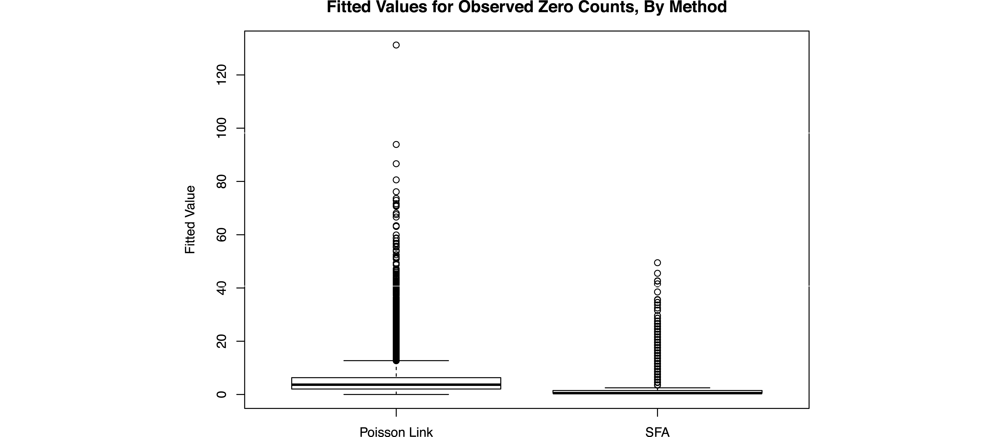
Accounting for zero inflation. This figure presents the fitted values for the 38,585 cases of an observed zero count in the legislator-term matrix for a Poisson density over term counts (left) and SFA (right). Of these zero counts, SFA gives a fitted value of below one for 23,532 of them, versus 3037 for the Poisson model. The marginal density used by SFA better fits the zeros in this data than does the Poisson model.

While we have taken a semiparametric approach to the marginal distribution over term frequencies, we note that Poisson densities (Chib and Winkelmann Reference Chib and Winkelmann2001) have also been used as the marginal densities of Gaussian copula models. We prefer
 $\widehat{F}(c)$
because even compared with a Poisson model that has been adjusted for zero inflation,
 $\widehat{F}(c)$
better accommodates the empirical term frequencies than would Poisson marginals. To illustrate, we fit both SFA and a latent Poisson model, implemented using the Wordfish algorithm of Slapin and Proksch (Reference Slapin and Proksch2008) and Lo, Proksch, and Slapin (Reference Lo, Proksch and Slapin2014), to the term-document matrix for floor speeches from the 112th Senate. Though we describe the data from our example more fully below, we bring it up now to compare the two methods. Figure 1 presents boxplots of the fitted values for the 38,585 cases of an observed zero count in the legislator-term matrix for a latent Poisson model (left) and SFA (right). Of these zero counts, SFA gives a fitted value of below one for 23,532 of them, versus only 3037 for the Poisson model.Footnote
6
The more flexible marginal density allows SFA better to fit the in-truth-zero terms, a key attribute of the data.
2.2.6 Prior sensitivity
The sensitivity of posterior inference to prior parameter specification is a generic concern for Bayesian models. With the exception of parameters about which the existing scaling literature has developed standard priors (e.g., Lauderdale and Clark Reference Lauderdale and Clark2014, Section 3.2) we select noninformative prior densities for our parameters. One component of our model, the Bayesian LASSO, uses two hyperprior parameters set by the researcher. We take as our hyperprior parameters on the Gamma prior those used in the literature (Park and Casella Reference Park and Casella2008; Kyung et al.
Reference Kyung, Gill, Ghosh and Casella2010), namely a shape of 1 and rate of 1.78. This prior expresses the expected size of effects we would expect to see, on a
 $z$
-scale. This prior captures the belief, before seeing the data, that we will see effects of size about
 $1/1.78\approx 0.57$
. We encourage varying these parameters to assess posterior sensitivity, which our software allows. We illustrate in the example below.
2.2.7 Balancing words and votes
As there are often an order of magnitude more terms than votes, the researcher may fear that the term data is swamping the vote data. We therefore introduce a parameter,
 $\unicode[STIX]{x1D6FC}$
, that controls the relative information coming from each source.Footnote
7
At
 $\unicode[STIX]{x1D6FC}=0$
, all information on the scaled locations comes from votes; at
 $\unicode[STIX]{x1D6FC}=1$
, all information on the scaled locations comes from words. Even when using information from only text or only votes, SFA offers additional insight over existing methods. When scaling off only the votes, SFA will place words in the same latent space as the votes, giving an ordering to terms driven by the vote information. This can help the researcher interpret the latent dimension, through finding words that are extreme in the vote dimension. Scaling the two datasets separately does not allow one dataset to inform the other.
We suggest three ways to select
 $\unicode[STIX]{x1D6FC}$
. The first involves fitting
 $\unicode[STIX]{x1D6FC}$
at a range of values and present the results, showing how they change along these shifts. This is the strategy we follow in our example below, presenting results for
 $\unicode[STIX]{x1D6FC}\in \{0,1/2,1\}$
. As a default, we suggest this strategy, unless the researcher has a substantive reason to select
 $\unicode[STIX]{x1D6FC}$
by one of the data-driven strategies below.
As a second strategy, we suggest selecting
 $\unicode[STIX]{x1D6FC}$
such that the ideal points are maximally discriminatory.Footnote
8
Denote as a function of
 $\unicode[STIX]{x1D6FC}$
both the dimension weights
 $a_{d}(\unicode[STIX]{x1D6FC})$
and the most preferred outcomes
 $x_{ld}(\unicode[STIX]{x1D6FC})$
. Our criterion favors strong dimensions
 $(\text{large values of }\{a_{d}(\unicode[STIX]{x1D6FC})\}_{d=1}^{D})$
as well as ideal points
 $(\{x_{ld}\}_{(l,d)=(1,1)}^{(L,D)})$
that provide maximal discrimination among individuals. The criterion we suggest is:
 $$\begin{eqnarray}\text{disc}(\unicode[STIX]{x1D6FC})=\mathop{\sum }_{d=1}^{D}\mathop{\sum }_{l=1}^{L}\mathop{\sum }_{l^{\prime }=1}^{L}a_{d}(\unicode[STIX]{x1D6FC})^{2}(x_{ld}(\unicode[STIX]{x1D6FC})-x_{l^{\prime }d}(\unicode[STIX]{x1D6FC}))^{2}\end{eqnarray}$$
with
 $\unicode[STIX]{x1D6FC}$
chosen to make the left-hand side of equation (13) as large as possible. All the elements needed to calculate
 $\text{disc}(\unicode[STIX]{x1D6FC})$
are returned from the MCMC output, so our software returns the full posterior density of this statistic, and the optimal value can be selected on the basis of which has the highest mean discrimination.
As a third criterion, we also implement the WAIC statistic, a Bayesian approximation of cross-validated prediction performance (Vehtari, Gelman, and Gabry Reference Vehtari, Gelman and Gabry2017). Though we favor a default of
 $1/2$
and of presenting results from
 $\unicode[STIX]{x1D6FC}$
of both 0 and 1, our discrimination and WAIC statistic give a means of a data-driven means of selecting
 $\unicode[STIX]{x1D6FC}$
. We illustrate the use of the discrimination and WAIC statistics in the online supplemental materials.
2.2.8 Software
We offer two implementations of the software. The first is a full MCMC implementation, which generates samples from the full posterior given the data. This allows the researcher to not only estimate the spatial locations as well as the number of latent dimensions, but also to characterize the uncertainty estimates. The second is an EM implementation. While it only returns point estimates, it is faster than the MCMC implementation and often useful for preliminary results during the process of practical modeling.Footnote 9
2.2.9 Additional uses
We have focused on a situation where both votes and term counts are present. There are cases where we observe legislative speech, but we either lack their votes or the votes are so heavily whipped we do not trust them. In this case, as we show in the context of our Congressional data, SFA can leverage words to recover reliable ideal point estimates even in the absence of reliable vote data for nonparty leaders.
Moreover, SFA estimates the spatial location of terms. Existing studies estimate the political affect of terms by attributing left leaning content to those used by Democrats, and rightward import to those spoken by Republicans (Laver, Benoit, and Garry Reference Laver, Benoit and Garry2003; Gentzkow and Shapiro Reference Gentzkow and Shapiro2010), or modelers posit that terms and votes arise from two conditionally independent data generating processes (Gerrish and Blei Reference Gerrish, Blei, Pereira, Burges, Bottou and Weinberger2012; Lauderdale and Clark Reference Lauderdale and Clark2014). SFA scales terms and votes simultaneously, providing natural structural estimates of word affect.
2.3 A discussion of our assumptions
Before considering any statistical method, the researcher should check that the assumptions of the model seem plausible in the study at hand. SFA extends the standard quadratic-loss spatial random utility model (Ladha Reference Ladha1991; Clinton, Jackman, and Rivers Reference Clinton, Jackman and Rivers2004) to encompass speech.Footnote 10 Though SFA can be fit to any data combining votes and text, we next consider the assumptions that allow us to interpret the results as estimates of preference parameters.
Behaviorally, our model assumes legislator
 $l$
’s votes and speech are both chosen as if she sincerely held an ideal point of
 $\{x_{ld}\}_{d=1}^{D}$
. It may be that these preferences are in fact sincere, but the posited behavior is also entirely consistent with the legislator seeking to convince her constituents that she behaves as if she held such preferences. Even if the agenda is structured so that members vote strategically on amendments, the ideal point estimates remain unbiased, though strategic voting does affect the interpretation of the bill parameters (Poole and Rosenthal Reference Poole and Rosenthal1997, p. 228). Likewise, the legislator speaks as though her preferred outcome was
 $\{x_{ld}\}_{d=1}^{D}$
. This may in fact be a tissue of lies, what matters for our purposes is that she speaks consistently as if she actually held the beliefs she claims to, and in particular that her preference parameters are impervious to being changed by persuasion.
SFA also requires two underlying structural assumptions. First, like the standard vote model, the SFA vote model requires an exogenous agenda, while the term model requires that the relevance of different terms be set exogenously. In both cases, the model assumes that all actors are “agenda-takers” rather than “agenda-setters.” Second, also like the standard vote model, the SFA vote model assumes that the legislators all agree about the spatial locations of the exogenously given status quo and alternative positions associated with each vote (Ladha Reference Ladha1991, esp. Section 2), and about the political content of each term they utter. Basically, words have to mean something, everyone has to agree approximately on what they mean, and that meaning cannot change over the period under study. This will typically be the case for people operating in the same legislature during the same session. The assumption becomes more problematic when applied across distinct contexts and widely different time periods. The payoff from placing the latent speech and voting variables together in a common space is that we can use both sources of information to obtain more precise estimates of legislators’ spatial preference parameters.
Even when these assumptions hold, the spatial preferences recovered by our estimator may correspond to a nonideological attribute. Of course, the resulting estimated locations are no less a reflection of preference for corresponding to nonideological traits. For example, in our analysis below, the second dimension we identify reflects differences between the vocabulary of party leaders and rank-and-file members. In this case the most preferred vocabulary of leaders is consistent with conducting business, assigning bills to committees, and organizing votes, while for other legislators it is not. Nevertheless, our framework captures this difference as a spatial attribute.
SFA, or any scaling method for that matter, should only be applied in situations where the assumptions seem reasonable given substantive knowledge. For example, we apply the method to US Senate floor speeches, noting that members of Congress are notorious for “dying with their ideological boots on” rather than changing positions on the issues (Poole Reference Poole2007). We would be less comfortable applying the method to judicial argument, in which case judges if not litigants likely do change their views. In Section 3, we apply our estimator to Congress, and we implement several methods for assessing internal and external validity, methods that analysts might want to use as checks when using SFA.
2.3.1 Topic models and related methods
We note that our method differs from the popular topic model approach to text analysis (Blei, Ng, and Jordan Reference Blei, Ng and Jordan2003; Grimmer Reference Grimmer2010; Roberts et al. Reference Roberts, Stewart, Tingley, Lucas, Leder-Luis, Gadarian, Albertson and Rand2014). In brief, when a researcher is looking for an underlying latent structure ordering actors and their choices, and they are comfortable making the model’s assumptions, then SFA should be implemented. In the absence of any structural or behavioral assumptions, topic models will always return a summary of clusters within the data. We emphasize that this is not an either/or distinction; SFA and topic models calibrate disparate features of the data.
Lastly, we situate SFA in the context of several other related methods. Many scholars have combined voting data with a topic model (Gerrish and Blei Reference Gerrish, Blei, Pereira, Burges, Bottou and Weinberger2012; Wang et al. Reference Wang, Salazar, Dunson and Carin2013; Lauderdale and Clark Reference Lauderdale and Clark2014). The methods, particularly when applied to courts, offer great insight: we may think of courts as voting on a wide array of topics, and judicial preference may vary greatly from one to the next. These models differ from SFA in two crucial aspects. First, the topic model methods do not give an ideological position to terms. Terms are not placed on, say, a left–right dimension shared by the actors. The topic models capture what actors are voting about, but not the ideological structure of the topics. Second, the models offer a disjointed relationship between words and votes. Actors are choosing both words and votes, but only vote choice is grounded in a spatial model. SFA differs by offering a tight, and formal, coupling of the ideological preferences that generate terms and votes. SFA is a model for term selection that is fully compatible with the standard and accepted models of vote choice.
2.3.2 Comparison with additional methods
SFA is related to several existing methods for scaling votes, scaling text, and combining multiple outcomes in a single factor analytic model. Our model is an extension of Ladha (Reference Ladha1991) and Clinton, Jackman, and Rivers (Reference Clinton, Jackman and Rivers2004) who model votes in a latent space, which they connect with binary choice using a probit model, and of Slapin and Proksch (Reference Slapin and Proksch2008) and Lo, Proksch, and Slapin (Reference Lo, Proksch and Slapin2014) who model spatial choice in a Poisson framework. Here we connect the latent space with count as well as binary outcomes (Murray et al. Reference Murray, Dunson, Carin and Lucas2013). Our estimation technique relies on probabilistic principal components analysis (Tipping and Bishop Reference Tipping and Bishop1999), whereby singular vectors and latent factors correspond if the errors are assumed independent and identically Gaussian. The method is factor analytic, as opposed to a singular value decomposition, because the scaling takes place in a latent space rather than operating directly on the observed data. We connect the two spaces using a Gaussian copula for mixed data.
Rather than matrix decompositions in a latent space, several works have turned to a Poisson or negative binomial model in order to model term counts. For example, Wordfish of Slapin and Proksch (Reference Slapin and Proksch2008), Lo, Proksch, and Slapin (Reference Lo, Proksch and Slapin2014) is similar to SFA, for terms, but under a Poisson or negative binomial link instead of a probit link. SFA leads to an identical formulation for the latent systematic component of word choice, except the latent component is exponentiated in order to guarantee positivity (see also Elff Reference Elff2013; Bonica Reference Bonica2014). SFA differs in that it places both word and vote choice in the same latent z-space, allowing both types of data to be modeled jointly. Our cut point model allows for a more flexible mapping from the latent to observed data space. We also model the zero inflation directly and are robust to outliers, as described above. SFA also estimates the underlying dimensionality.
The use of the Poisson by Slapin and Proksch (Reference Slapin and Proksch2008) notwithstanding, many analysts eschew both the Poisson and the Negative Binomial in their analysis of text. Examples include: the widely used Wordscores model of Laver, Benoit, and Garry (Reference Laver, Benoit and Garry2003) or the nonparametric content analysis of Hopkins and King (Reference Hopkins and King2010); the text based “slant” measures used by Gentzkow and Shapiro (Reference Gentzkow and Shapiro2010); the LDA formulation of Blei, Ng, and Jordan (Reference Blei, Ng and Jordan2003), Gerrish and Blei (Reference Gerrish and Blei2011) which converts term counts to proportions, thereby admitting a Dirichlet prior; PCA or kernel PCA on the tf-idf matrix Spirling (Reference Spirling2012); and semiparametric copula models for mixed data Hoff (Reference Hoff2007). Like these, SFA is not based on a Poisson model; see Murray et al. (Reference Murray, Dunson, Carin and Lucas2013, esp. 2.1) for a formulation close to SFA’s.
Mixed factor analysis models have turned to copulas to combine data of different types. In these models, mixed data such as counts, binary, and continuous data, are placed on and analyzed on a common underlying latent scale. The Gaussian copula, which places all data on an underlying common
 $z$
-scale, is a typical choice. For example, Quinn (Reference Quinn2004) converts observed continuous data to a
 $z$
-scale, and then combines it with ordinal and categorical data on the same scale; for recent extensions, see Hoff (Reference Hoff2007), Murray et al. (Reference Murray, Dunson, Carin and Lucas2013). Our model is closely related to that given in Murray et al. (Reference Murray, Dunson, Carin and Lucas2013, Section 2.1). We differ in that we only have two types of data, text and votes, and hence have to estimate only one set of cutpoints, whereas Murray et al. (Reference Murray, Dunson, Carin and Lucas2013) consider the problem of generic types of data. Murray et al. (Reference Murray, Dunson, Carin and Lucas2013) work with the transformed ranks of all variables, eschewing cutpoints entirely. For that reason, our method is more powerful when modeling votes and text. SFA also introduces a cut point modeled tailored to several common aspects of text data, as we describe above.
Other methods have estimated dimensionality (Heckman and Snyder Reference Heckman and Snyder1997; Hahn, Carvalho, and Scott Reference Hahn, Carvalho and Scott2012). Additionally, Aldrich, Montgomery, and Sparks (Reference Aldrich, Montgomery and Sparks2014) show that sufficiently large cross-party variance can mask important within-party dimensions.Footnote 11
3 Illustrative Application: The US Senate, 1997–2012
In this section, we apply SFA to recent US Senate data. The analysis proceeds in three steps. First, we describe the data and discuss the viability of SFA in this context. Second, we apply the method to the contemporary US Senate. Third, we simulate a “strong-party” system where we use SFA to use text data to gain leverage on rank-and-file ideal points even in the presence of party line voting and heavy missingness in the vote data.
3.1 Data
We apply SFA to the eight recent sessions of the US Senate. We scale using both votes and words, returning both ideology estimates and our calibration of the underlying dimensionality. Our data come from two sources. Rollcall data come from VoteView.Footnote 12 For the text data, we rely on floor speeches as gathered by the Sunlight Foundation.Footnote 13 Following standard practice (e.g., Quinn et al. Reference Quinn, Monroe, Colaresi, Crespin and Radev2010; Grimmer and Stewart Reference Grimmer and Stewart2013), we stem, eliminate stop words, and model unigrams and bigrams. Both vote and speech data are polled over the full session. We trim all terms that are not used by at least ten people at least ten times over the course of the session.Footnote 14
Before applying the method, let us consider the applicability of SFA in this case. First, voting is not always sincere in the US Senate, as there are always motions to recommit, etc. We note, though, that ideal point estimates from the US Congress have been used extensively in other studies and possess high face validity. To be particularly careful, if a bill is voted on several times due to different motions, we only include the final vote in our analysis.
Second, we consider the sincerity when speaking. Previous work has shown, albeit in the US House, that floor speeches are expressive rather than deliberative (Maltzman and Sigelman Reference Maltzman and Sigelman1996; Hill and Hurley Reference Hill and Hurley2002). Many floor speeches are not even read verbally, but simply entered into the record, also suggesting that floor speeches are vehicles of expression rather than persuasion. For that reason, we feel more comfortable applying the method to floor speeches rather than, say, conference committee meetings.
3.2 Results
We present three sets of results. Each corresponds with the proportion of information in the votes coming from votes instead of words (
 $\unicode[STIX]{x1D6FC}\in \{0,1/2,1\}$
). We present results on the estimated number of dimensions and interpretation of each.
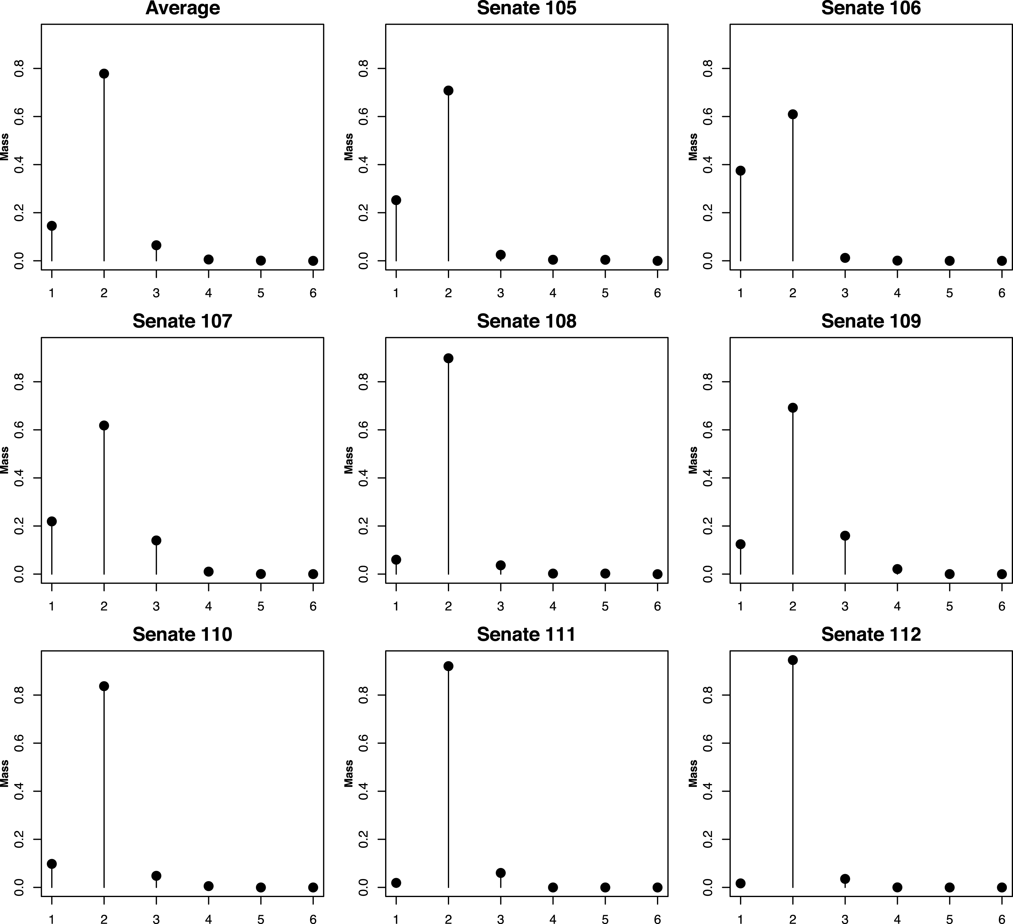
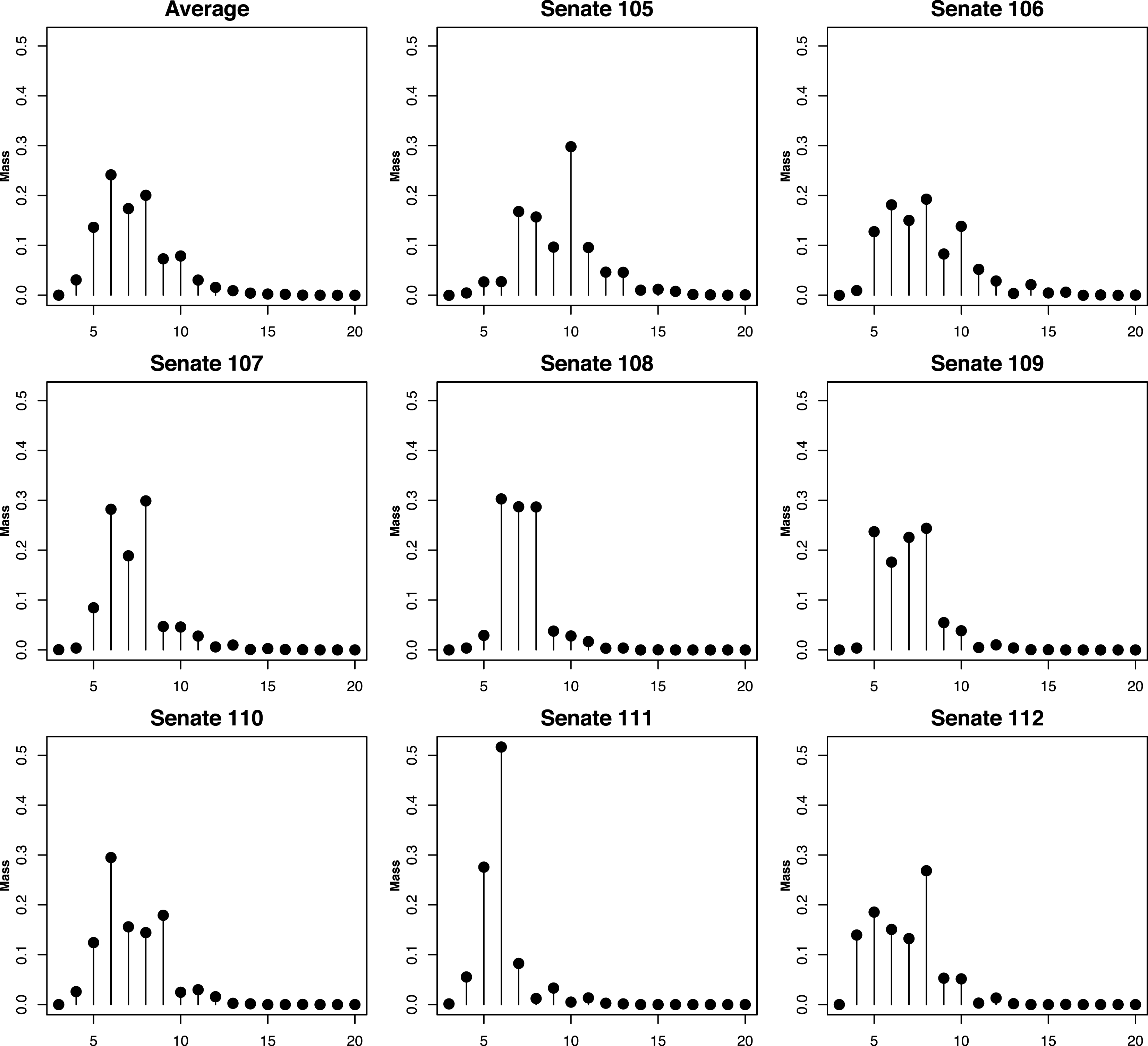
Posterior density over number of underlying dimensions for the joint word and vote model. We find a pronounced mode at two dimensions consistently across Senates. The average across all Senates appears in the top left corner.

3.2.1 Scaling results informed only by votes (
 $\unicode[STIX]{x1D6FC}=0$
)

We begin with the model with information coming only from votes. This model places a posterior mass estimate from 99.96% to 100% on one dimension for each Senate. Posterior means of ideal point estimates correlate with DW-NOMINATE estimates ranging from 0.953 to 0.980 across the eight Senates analyzed here (see the first dimension of Figure 4 below).
3.2.2 Scaling results informed by words and votes (
$\unicode[STIX]{x1D6FC}=1/2$
)

We next move on to the model that gives equal weight to words and votes. First, we consider the estimated number of dimensions, see Figure 2. The average density over the number of dimension parameters merging all Senates is in the top left corner, while the successive sessions are depicted from top to bottom and from left to right. A pronounced mode at two dimensions reappears consistently across Senates.
Not only is the finding of two dimensions consistent, but the two dimensions themselves are stable across sessions. The first closely coincides with the standard ideology dimension uncovered from scaling roll call votes. The second appears to be a leadership dimension, with party leaders at one end while a variegated mix of rank-and-file partisans and ideological moderates populate the other.
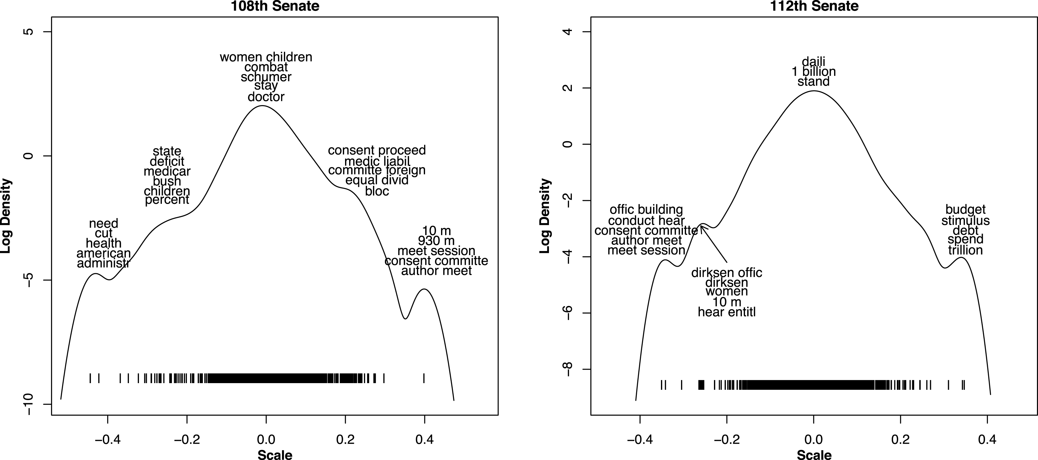
Log density of term weights, after scaling votes and terms together. The weights are oriented such that terms more likely to be spoken by Republicans are to the right. Each local mode is labeled by the terms closest to that mode. The left figure presents results from the Republican controlled 108th Senate, the right figure contains results from the Democratic-led 112th Senate.

Figure 3 presents the log density of term weights, after scaling votes and terms together. The weights are oriented such that terms more likely to be spoken by Republicans are to the right. Each local mode is labeled by the five terms closest to that mode. The left figure contains results from the 108th Senate, a Republican-led session during President George W. Bush’s tenure. The right figure contains results from the 112th Senate, a Democratic-led session during President Barack Obama’s time as President.
We find a consistent pattern: for the majority party, the most extreme terms relate to parliamentary control words (consent committee, author meet, meet session). For the minority party, the first dimension identifies ideologically relevant terms. For the Democrats during the 108th Senate, these terms included administr, as the Democrats soured on the current Presidential administration, and health, a centerpiece of the Democratic policy agenda. In the 112th Senate, with the Democrats in the majority, parliamentary control terms switched their ideological polarity, aligning with the Democrats (meet session, consent committee, author meet). The Republican end of this first dimension reflects that party’s programmatic fiscal concerns (budget, stimulus, debt, trillion).
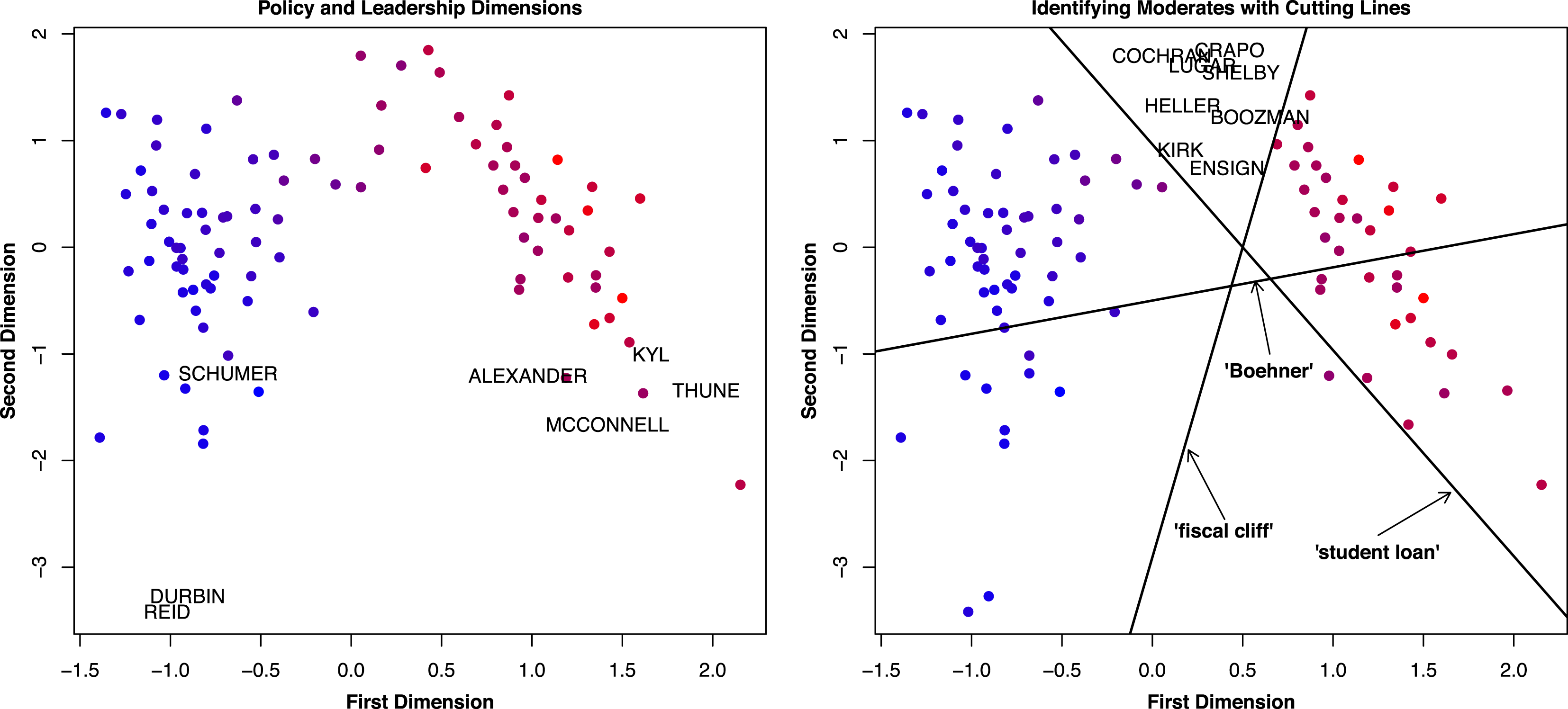
Next, we look at the preferred outcomes of legislators from the 112th. Points in Figure 4 are shaded in proportion to their first dimensional DW-NOMINATE score, showing the agreement between SFA and DW-NOMINATE on the first dimension (
 $\widehat{\unicode[STIX]{x1D70C}}\approx 0.93$
). The left plot labels party leaders, whips, and top chairmen, showing the close relationship between locations on the second dimension and leadership. The first dimension captures the political battle lines, reflecting legislators left versus right policy differences, while the second, vertical, dimension reflects differences in the terms selected by leaders versus the rank-and-file members.
Latent dimensions estimated by SFA, 112th Senate. Legislators’ preferred outcomes on the first dimension (
 $x$
-axis) and the second (
 $y$
-axis). The left plot labels party leaders, whips, and top chairmen. In the right plot cutting lines separate frequent from infrequent users, of the terms: Boehner, student loan and fiscal cliff.

The right plot of Figure 4 contains cutting lines for three terms: Boehner, student loan, and fiscal cliff. The lines were constructed such that legislators on one side are expected to use the phrase above the median number of its raw usage, and on the other side legislators are expected to use the word below its median number of times. We find leaders are more likely to use the word Boehner, the House Speaker during this session. Republicans were more likely to use the term fiscal cliff, with leaders the most likely. Democrats were more likely to utter the phrase student loan, again with leaders the most likely to employ the term. SFA identifies a group of Republican moderates in the top V, here we label them by name. These moderates are not likely to use either student loan or fiscal cliff.
Concerned about prior sensitivity, we also varied the LASSO prior parameters by a factor of
 $(0.25,0.5,1,1.5)$
, generating 16 different runs. We find similar results, with scaled locations across the settings correlating above 0.95, on average. When we select these parameters by the WAIC, we find the same results as those presented here: two stable dimensions, and again scaled locations correlating with those estimated below above 0.95.
3.2.3 Scaling results informed by only words (
$\unicode[STIX]{x1D6FC}=1$
)

Estimated underlying dimensionality for Senate floor speeches. Results across all sessions are in the top left corner and remaining sessions follow.

We also apply SFA using only information from words. This is not our preferred model, as it ignores vote data, yet SFA still uncovers structure in the text data. The posterior density of estimated dimensionality for pooled floor speeches can be found in Figure 5. Results across all sessions are in the top left corner while the remaining sessions follow in order from top to bottom and from left to right. In contrast with the high concentration of probability on two dimensions in our preferred model, when we exclude the valuable information contained in votes and analyze oratory alone, we obtain a somewhat more diffuse density that accords a 75% probability to there being between five and eight dimensions, and a probability of over 95% that the underlying dimensionality is within the range
 $[4,11]$
. Looking at individual sessions, we find a similar dimensionality, albeit with some year-to-year variation.
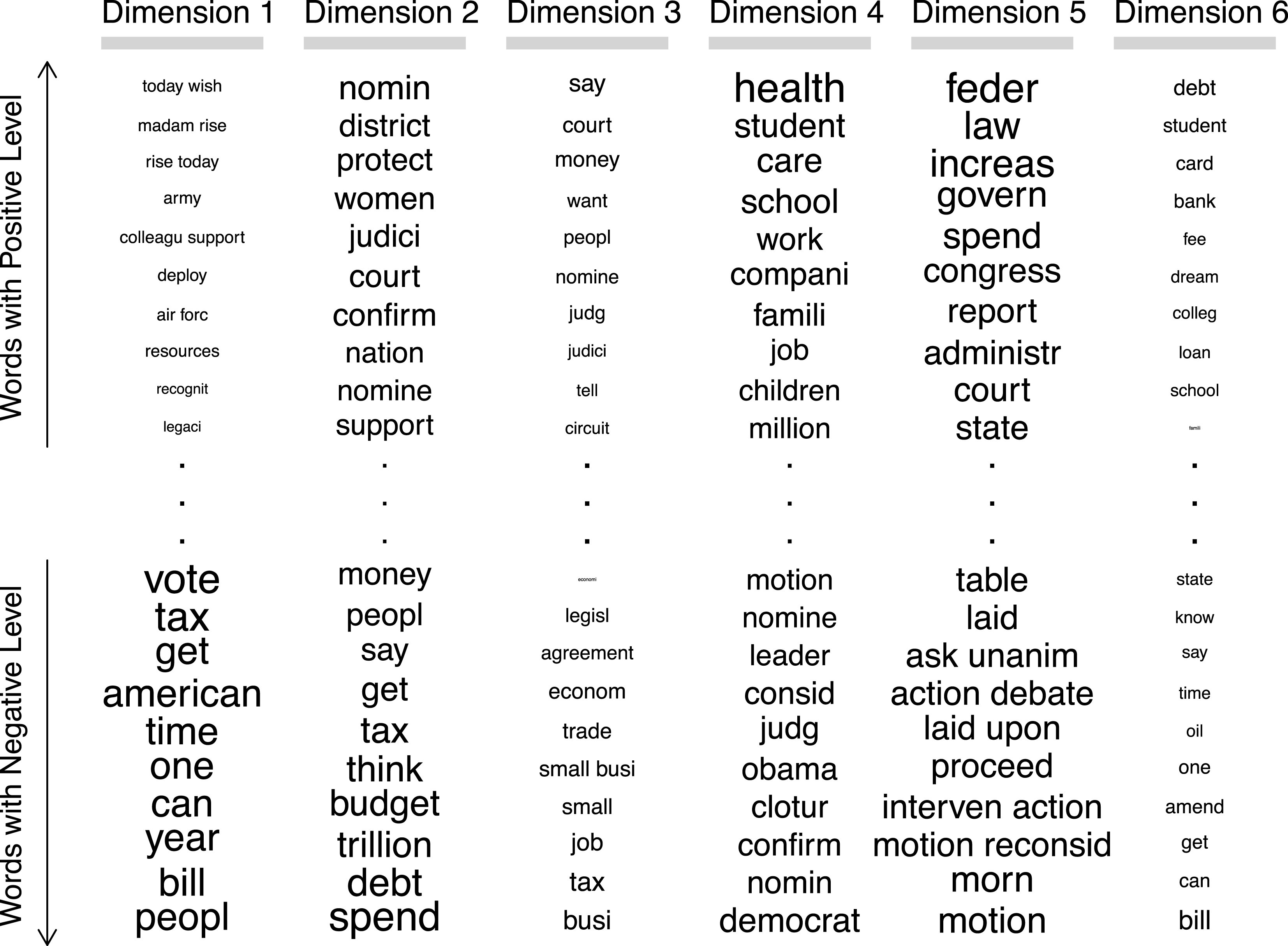
Extreme terms by dimension, 112th Senate. Extreme terms for the first six dimensions as estimated by SFA from the 112th Senate. The type size of each term is proportional to the absolute value of the associated coefficient; terms earning positive coefficients appear in the upper part of the panel, those assigned negative coefficients are presented in the lower segment.

Figure 6 contains the top ten words at each of the first six dimensions of the 112th Senate. We note that the positive and negative level distinction along the
 $y$
-axis is wholly arbitrary, as we only identify term levels up to a sign. Looking at the first column, we find that the first dimension starts with a set of noncontroversial terms. These include parliamentary procedural terms (as opposed to parliamentary control terms) such as today wish, madam rise, and colleague support. Also on the noncontroversial side are martial terms with universally positive affect during this Congress such as army, air forc, and deploy. On the other side are words that will be used to differentiate issues in other dimensions, such as tax, vote, and peopl. The other dimensions have at their extremes words connoting some underlying dimension of policy. For example, the second dimension ranges from judiciary and women’s issues at one end to fiscal concerns at the other; the fourth goes from a broad set of social welfare concerns to the consideration of judicial nominees. These lower dimensions adapt to the issues of the day. Tobacco, for example is present in the 105th Senate; Iraq comes and goes as an issue, and health care goes from dealing with seniors and Medicare in the 107th Senate to dealing with students and families in the 112th. Even without including votes in our analysis, SFA selects a relatively parsimonious and informative representation of the Senate.
3.2.4 Extension: imputing estimates for members’ given only votes from leadership
We next offer a possible extension of SFA. In a strong-party system, legislators vote their party’s rather than their own preferences (e.g., Kellerman Reference Kellerman2012). In these cases, votes may not be a trustworthy measure of preference, but legislative speech may help provide leverage. To simulate this scenario, we coded all vote data except for the party leaders and whips as missing, while maintaining all speech data. This left a vote record for less than 4% of the Senate. We then compared the SFA ideal point estimates to the SFA estimates using everyone’s speech, but only leaders’ votes.
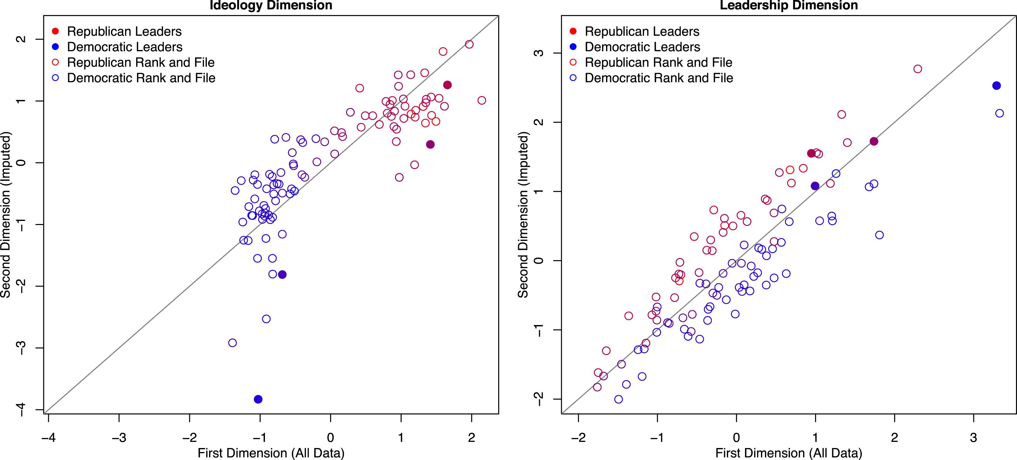
Estimated ideology when only leaders votes are informative. The voting dimension estimates appear in the left panel, with the censored estimates measured on the vertical (
 $y$
-axis) while the uncensored ones appear on the horizontal (
 $x$
-axis). In the censored data the salience of the voting dimension drops, so that it becomes the second dimension. The right hand panel exhibits the leadership dimension, again the censored estimates correspond with the vertical (
 $y$
-axis) and the uncensored ones coincide with the horizontal (
 $x$
-axis).

Results are present in Figure 7. We again recover two dimensions, but as we have dropped over 95% of our observed vote data, the order has flipped. Our first dimension is now driven by words and the second by votes. The left panel of the figure compares estimates for the voting dimension, which is the second dimension estimated with the heavily censored data (plotted along the vertical
 $y$
-axis) versus the first dimension of the uncensored estimates (along
 $x$
-axis). Observations are labeled by party, and leaders’ locations are solid.
As expected, with so little voting data, recovery of the first dimension is far from perfect, but remarkably the imputed scores correlate highly, at more than 0.79. This effect is not simply a cross-party effect due to extreme partisanship; the within-party correlations are more than 0.4.
The right hand panel compares estimates for the “leadership” dimension, the first dimension in the censored data but the second in the full data. The censored estimates correspond closely with their uncensored counterparts, as this dimension is driven primarily by words and these were not censored.
4 Conclusion
We propose a method, Sparse Factor Analysis, for combining votes and text data in a single scaling procedure. The method models both word choice and vote choice in terms of the same ideal points. Furthermore, we develop a statistical framework that allows us to estimate both individuals’ most preferred outcomes and the underlying dimensionality of the joint word–vote space. The resulting methodology provides a close linkage between the choice-theoretic models of vote and word choice. This tight connection allows the extension of SFA to more complex decision scenarios (e.g., Clinton and Meirowitz Reference Clinton and Meirowitz2003). SFA allows the analyst to estimate the underlying number of latent dimensions, rather than having to impose dimensionality a priori.
Substantively, we analyze legislative speech and roll call voting from eight recent sessions of the US Senate. Combining both data sources reveals a consistent picture of a two-dimensional Senate, with the first dimension coinciding with the voting dimension, while the second distinguishes leaders of both parties from the rank and file.
While SFA is designed to analyze individuals who both speak and cast votes, it allows us to impute policy preferences to non-voting political speakers.Footnote 15 This may prove useful in confronting the perennial research problem of imputing the preferred policy outcomes of legislative candidates. While analysts can impute the ideology of victorious candidates from their subsequent congressional conduct, as they can infer the leanings of defeated incumbents from their previous voting records, measuring the preferences of defeated challengers has proven to be a more elusive goal. Yet every challenger spends time and energy generating political speech. SFA offers the possibility of imputing the most preferred policy such a candidate would have pursued had he been elected.
We hope the approach in this paper also finds purchase beyond the US Congress. For example, in strong-party systems where votes are relatively uninformative, words may be used to help clarify the within-party variance in ideal points. We are currently exploring applications of the method in situations where voting is not perfectly reflective of underlying individual preference or where ideal points are allowed to evolve over time.