1. Introduction
Multiphase flows are ubiquitously observed in nature, daily life and widely applied in various engineering applications, such as spray drying, ink-jet printing, oil recovery, etc. (Jalil & Hussein Reference Jalil and Hussein2019; Lohse Reference Lohse2021).They typically consist of two or more liquid or gas flows accompanied by complicated motions and deformations of liquid–gas interfaces. Due to high complexity, advanced modelling of multiphase flows has long been a challenging task. Situated at a mesoscopic scale, the lattice Boltzmann method (LBM) directly solves the discrete kinetic equation. Due to its kinematic nature, LBM can automatically capture the interfacial dynamics by incorporating intermolecular-level interactions. Therefore, it has become very popular and achieved remarkable successes in modelling and studying complex multiphase flows in the last few decades (Grunau, Chen & Eggert Reference Grunau, Chen and Eggert1993; Chen & Doolen Reference Chen and Doolen1998; Aidun & Clausen Reference Aidun and Clausen2010; Chen et al. Reference Chen, Kang, Mu, He and Tao2014; Li et al. Reference Li, Luo, Kang, He, Chen and Liu2016; Hosseini & Karlin Reference Hosseini and Karlin2023). There are typically four categories of LBMs to model multiphase flows, i.e. the free energy model (Swift et al. Reference Swift, Osborn and Yeomans1995, Reference Swift, Orlandini, Osborn and Yeomans1996), the colour-gradient model (Gunstensen et al. Reference Gunstensen, Rothman, Zaleski and Zanetti1991; Liu et al. Reference Liu, Lu, Li, Yu and Sahu2021), the phase field model (Zu & He Reference Zu and He2013; Zhu et al. Reference Zhu, Kou, Yao, Li and Sun2020) and the Shan–Chen pseudopotential model (Shan & Chen Reference Shan and Chen1994; Shan Reference Shan2008). Among them, the pseudopotential model has become very popular, due to its simplicity and versatility.
In the pseudopotential model, intermolecular interactions are modelled by a density-based pseudopotential, while phase separation is realised by attraction between the current lattice and its neighbours. Despite the simplicity and versatility, the pseudopotential model suffers from several strong disadvantages. The primary disadvantage is the violation of thermodynamic consistency, i.e. the liquid–vapour co-existence densities deviate from the Maxwell construction. To solve this problem, Li, Luo & Li (Reference Li, Luo and Li2012) proposed an improved force term to tune the mechanical stability, and achieved good thermodynamic consistency at high liquid–vapour density ratios. Kupershtokh, Medvedev & Karpov (Reference Kupershtokh, Medvedev and Karpov2009) proposed an mean-gradient force scheme by a linear combination of two pseudopotentials, which has also been verified in achieving thermodynamic consistency (Gong & Cheng Reference Gong and Cheng2012). In addition, the thermodynamic consistency can also be improved by modifying the equation of state (EoS), such as the piecewise EoS (Colosqui et al. Reference Colosqui, Falcucci, Ubertini and Succi2012) and the customised EoS (Peng et al. Reference Peng, Ayala, Wang and Ayala2020). The second drawback is the high spurious current around the liquid–vapour interface, which may seriously affect the modelling accuracy. Sbragaglia et al. (Reference Sbragaglia, Benzi, Biferale, Succi, Sugiyama and Toschi2007) found that the spurious current can be reduced by using high-order isotropic gradient operators (Shan Reference Shan2006). By decreasing the attraction parameter in the EoS, the spurious current can also be reduced (Qin et al. Reference Qin, Moqaddam, Ali, Qinjun and Carmeliet2018). Hu et al. (Reference Hu, Li, Chen, Liao and Zeng2013) proposed multiplying the pressure by a prefactor smaller than unity, which is also validated as effective in reducing the spurious current. However, all these methods share the disadvantage of thicken the liquid–vapour interface to some extent. The third disadvantage is not limited to the pseudopotential model itself but to all the LBMs, which is their disability in reaching low fluid viscosity. To improve this situation, several advanced collision operators are developed, such as the multiple-relaxation-time (MRT) model (Lallemand & Luo Reference Lallemand and Luo2000; D’Humieres et al. Reference D’Humieres, Ginzburg, Krafczyk, Lallemand and Luo2002), the entropic LBM (Mazloomi et al. Reference Mazloomi, Chikatamarla, S. and Karlin2015; Wöhrwag et al. Reference Wöhrwag, Semprebon, Moqaddam, Karlin and Kusumaatmaja2018), the entropic MRT LBM (EMRT or KBC) (Karlin, Bösch & Chikatamarla Reference Karlin, Bösch and Chikatamarla2014; Bösch et al. Reference Bösch, Dorschner and Karlin2018; Qin et al. Reference Qin, Moqaddam, Ali, Qinjun and Carmeliet2018; Hosseini et al. Reference Hosseini, Dorschner and Karlin2022, Reference Hosseini, Dorschner and Karlin2023; Xu et al. Reference Xu, Tian, Zhu and Zhao2024), the regularised LBM (Feng et al. Reference Feng, Boivin, Jacob and Sagaut2019), the non-orthogonal MRT LBM (Li, Yu & Luo Reference Li, Yu and Luo2019a ; Fei et al. Reference Fei, Du, Luo, Succi, Lauricella, Montessori and Wang2019) and the cascaded LBM (Fei et al. Reference Fei, Yang, Chen, Mo and Luo2020; Xu et al. Reference Xu, Tian, Zhu and Zhao2024), etc. With these advanced collision operators, flows with low fluid viscosity and/or high Mach number can be modelled.
Another critical drawback is the free adjustment of surface tension independent of the temperature/density ratio, since surface tension is essential to study multiphase flows. Sbragaglia et al. (Reference Sbragaglia, Benzi, Biferale, Succi, Sugiyama and Toschi2007) proposed a multirange pseudopotential to realise the tuneable surface tension. However, Huang, Krafczyk & Lu (Reference Huang, Krafczyk and Lu2011) found the density ratio varies when this model is applied. Li & Luo (Reference Li and Luo2013) proposed adding a source term using only the pseudopotential of the nearest neighbour. Their simulations show that the density ratio remains almost unchanged on tuning the surface tension. But this model is only applicable to MRT LBM. Lycett-Brown & Luo (Reference Lycett-Brown and Luo2015) applied a higher-order analysis to derive a general forcing term, using which they realised arbitrarily high density ratio and independent tuning of surface tension. However, the high-order terms are generally more complex. More recently, Kharmiani et al. (Reference Kharmiani, Niazmand and Passandideh-fard2019) proposed selecting two Taylor expansion terms as source terms of the pseudopotential LBM, and realised the maintaining of thermodynamic consistency as well as independent adjustment of surface tension. A drawback of their model, as analysed by Wang et al. (Reference Wang, Fei and Luo2022), is that, the calculation of the second term requires information from the second layer of neighbouring grids. Wang et al. (Reference Wang, Fei and Luo2022) improved this model by replacing the second source term with a modified combined pseudopotential. In their work, Wang et al. (Reference Wang, Fei and Luo2022) combined the model with the KBC collision operator, in order to realise low fluid viscosity. Very recently, Xu et al. (Reference Xu, Tian, Zhu and Zhao2024) combined a similar pseudopotential force with their enhanced cascaded KBC model, to achieve droplet impact on a flat surface with high Reynolds and Weber numbers. However, we note that, for the implementation of the KBC model (Wang et al. Reference Wang, Fei and Luo2022; Xu et al. Reference Xu, Tian, Zhu and Zhao2024) using Guo’s force scheme (Guo, Zheng & Shi Reference Guo, Zheng and Shi2002), the entropic stabiliser is calculated based on the equilibrium distribution function, while the external fluid–fluid and fluid–solid forces are not completely considered. An alternative force scheme is to use the exact difference method (EDM) (Kupershtokh et al. Reference Kupershtokh, Medvedev and Karpov2009), which is more general and applicable to different collision operators. For instance, by applying EDM, Qin et al. (Reference Qin, Moqaddam, Ali, Qinjun and Carmeliet2018) combined the KBC model with the multirange pseudopotential (Sbragaglia et al. Reference Sbragaglia, Benzi, Biferale, Succi, Sugiyama and Toschi2007) to realise adjustable surface tension. Bösch et al. (Reference Bösch, Dorschner and Karlin2018) also applied the EDM to couple KBC with the free energy model to simulate multiphase flow with adjustable surface tension. Similarly, Hosseini, Dorschner & Karlin (Reference Hosseini, Dorschner and Karlin2023) used EDM to combine KBC and a proposed pseudopotential to reproduce the correct Korteweg stress for modelling multiphase flows with adjustable surface tension. However, for these implementations using EDM, the adjustable range of surface tension is limited to only a few times of the original value. As a result, the modelled Weber number is limited to relatively small values of less than 330 (Qin et al. Reference Qin, Moqaddam, Ali, Qinjun and Carmeliet2018; Bösch et al. Reference Bösch, Dorschner and Karlin2018; Hosseini et al. Reference Hosseini, Dorschner and Karlin2023), which is not sufficient to model the complex droplet dynamics such as splashing (Zhang et al. Reference Zhang, Zhang, Yi, He, Niu and Hao2021a ). More importantly, compared with Guo’s scheme (Guo et al. Reference Guo, Zheng and Shi2002), the EDM force scheme introduces higher-order error terms (Li et al. Reference Li, Luo and Li2012; Moqaddam Reference Moqaddam2016), which seriously affect the pressure tensor in two-phase flows and also the adjustment of surface tension. However, the higher-order error terms are not considered in these works.
In the current work, while we still achieve the independent adjustment of surface tension, we tackle exactly the problem of previous work which did not fully consider the external forces in the KBC model. The solution is to apply EDM as the force scheme which could fully incorporate the influence of external forces on the stabiliser (Bösch et al. Reference Bösch, Dorschner and Karlin2018). The way of realising independent surface adjustment is to follow Wang et al. (Reference Wang, Fei and Luo2022). The main challenge of this work lies in the consideration of the higher-order terms, as we introduced above. In § 2, we first introduce the KBC model, then we theoretically derive how the higher-order error term affects the tuning of surface tension. Afterwards, in § 3, we first validate the improved model to independently tune the surface tension. Then we apply it to the complex multiphase dynamics of a droplet splashing on a thin liquid film and mesh structures. We could achieve Reynolds and Weber numbers of around one order of magnitude higher than reported in the literature. Further, we apply it to investigate the influence of surface wettability and the liquid–gas viscosity ratio on the splashing dynamics, as well as the influence of mesh opening size on the droplet spreading, penetration and splashing dynamics. Section 4 concludes the present work.
2. Numerical modelling
2.1. Single-phase EMRT (KBC) LBM
A general form of the lattice Boltzmann (LB) equation can be written as
 \begin{align} {f_i}({\boldsymbol {x}} + {{\boldsymbol {c}}_{\boldsymbol {i}}}\Delta t,t + \Delta t) = f_i^* = \left ( {1 - \beta } \right ){f_i}\left ( {{\boldsymbol {x}},t} \right ) + \beta f_i^{\textit{mirr}}\left ( {{\boldsymbol {x}},t} \right ), \end{align}
where
 $f_i$
is the discrete density distribution function,
 ${{\boldsymbol {c}}_{\boldsymbol {i}}} = ({c_{\textit{ix}}},{c_{\textit{iy}}})$
is the discrete velocity in the
 $i{\rm th}$
direction and
 $\Delta t$
is the time step. The mirror state
 $f_i^{\textit{mirr}}$
is vital for the model construction. In the frequently used lattice Bhatnagar-Gross-Krook (LBGK) model (Qian, D’Humières & Lallemand Reference Qian, D’Humières and Lallemand1992; Chen & Doolen Reference Chen and Doolen1998), the mirror state is written as
 $f_i^{\textit{mirr}} = 2f_i^{\textit{eq}} {-} {f_i}$
, where
 $f_i^{\textit{eq}}$
is the equilibrium density distribution function. In the KBC model, the density distribution function is basically split into three parts
 \begin{align} {f_i} = {k_i} + {s_i} + {h_i}, \end{align}
where
 $k_i$
is the kinematic part which depends on the locally conserved fields of mass and momentum,
 $s_i$
the shear part which involves the stress tensor and
 $h_i$
the higher-order moment which is not included in
 $s_i$
. In the KBC model, the key point is to find the proper
 $k_i$
,
 $s_i$
and
 $h_i$
of the mirror state distribution
 $f_i^{\textit{mirr}}$
. To conserve mass and momentum,
 $k_i^{\textit{mirr}}$
in
 $f_i^{\textit{mirr}}$
is kept the same as in
 $f_i$
. For the shear part
 $s_i^{\textit{mirr}}$
, it is set as
 ${s_i}={2s_i^{\textit{eq}} - {s_i}}$
to make the deviations from
 $f_i$
and
 $f_i^{\textit{mirr}}$
to the equilibrium
 $f_i^{\textit{eq}}$
the same (
 $\Delta s_i = {s_i} - {s_i^{\textit{eq}}} = {s_i^{\textit{eq}}} - s_i^{\textit{mirr}}$
) as in the LBGK model, in order to ensure the shear stress is correctly modelled. For the higher-order part
 $h_i^{\textit{mirr}}$
, its determination varies with different collision models. A generic form can be written as a linear combination of
 $h_i$
and its equilibrium
 $h_i^{\textit{eq}}$
, i.e.
 $h_i^{\textit{mirr}} = { ( {1 - \gamma } ){h_i} + \gamma h_i^{\textit{eq}}}$
. In this way, the mirror state can be written in a one-parameter form as
 \begin{align} f_i^{\textit{mirr}} = {k_i} + \left [ {2s_i^{\textit{eq}} - {s_i}} \right ] + \left [ {\left ( {1 - \gamma } \right ){h_i} + \gamma h_i^{\textit{eq}}} \right ]\!, \end{align}
where
 $\gamma$
is the free parameter that determines the model performance, which we will discuss later. The kinematic part
 $k_i$
is a fixed formula according to the conservation of mass and momentum. We apply the ‘KBC-N4’ formulation to implement
 $s_i$
, following Karlin et al. (Reference Karlin, Bösch and Chikatamarla2014) and Bösch et al. (Reference Bösch, Chikatamarla and Karlin2015). Take the two-dimensional nine-velocity (D2Q9) LBM for an example, to obtain
 $s_i$
, the first step is to construct moments of different orders by
 \begin{align} \rho {M_{pq}} = \sum \limits _{i = 0}^{Q - 1} {{f_i}c_{\textit{ix}}^pc_{\textit{iy}}^q} ,p,q \in \{ 0,1,2\}. \end{align}
For convenience, we use the following linear combinations to represent the natural moments to construct
 $s_i$
, i.e.
 $T=M_{20}+M_{02}$
,
 $N=M_{20}-M_{02}$
and
 ${\varPi _{\textit{xy}}} = {M_{11}}$
. With this set of natural moments, the shear part
 ${s_i} = {s_{({c_{\textit{ix}}},{c_{\textit{iy}}})}}$
can be uniquely represented as
 \begin{align} {s_{(0,0)}} = - T,{s_{({c_{\textit{ix}}},0)}} = - \frac {1}{4}(T + N),{s_{(0,{c_{\textit{iy}}})}} = \frac {1}{4}(T - N),{s_{({c_{\textit{ix}}},{c_{\textit{iy}}})}} = \frac {1}{4}{c_{\textit{ix}}}{c_{\textit{iy}}}{\varPi _{\textit{xy}}}. \end{align}
The expressions of
 $s_i$
in the three-dimensional 27-velocity (D3Q27) LBM are given in Appendix A. In the EMRT-LBM, the value of
 $\gamma$
is calculated based on minimisation of the discrete entropy
 $S [ {{f^*} ( \gamma )} ]$
of the post-collision state
 $f^*$
, i.e.
 \begin{align} \frac {{{\rm d}S({f^*}(\gamma ))}}{{{\rm d}\gamma }} = 0,S(f^*) = \sum \limits _{i = 0}^{Q - 1} {{f_i^*}\ln \left(\frac {{{f_i^*}}}{{{W_i}}}\right)} , \end{align}
where
 $W_i$
are the lattice weights and
 $W_0=4/9, W_{1-4}=1/9, W_{5-8}=1/36$
. Introducing
 $\Delta {s_i} = {s_i} {-} s_i^{\textit{eq}}$
and
 $\Delta {h_i} = {h_i} - h_i^{\textit{eq}}$
, the condition for the critical point, i.e. the derivative of entropy equal to zero as given in (2.6), can be reformulated as
 \begin{align} \sum \limits _{i = 0}^{Q - 1} -\beta {\Delta {h_i}\left \{ {1 + \ln \frac {{f_i^{\textit{eq}}}}{{{W_i}}}+\ln \left [ {1 + \frac {{\left ( {1 - \beta \gamma } \right )\Delta {h_i} - \left ( {2\beta - 1} \right )\Delta {s_i}}}{{f_i^{\textit{eq}}}}} \right ]} \right \}} = 0. \end{align}
As we know,
 $k_i$
is the kinematic part of the distribution function
 $f_i=k_i+s_i+h_i$
to conserve mass and momentum. Thus we simply obtain
 \begin{align} \begin{array}{*{20}{c}} {\sum \limits _{i = 0}^{Q - 1} {{f_i}} = \sum \limits _{i = 0}^{Q - 1} {f_i^{\textit{eq}}} = \sum \limits _{i = 0}^{Q - 1} {{k_i}} = \sum \limits _{i = 0}^{Q - 1} {k_i^{\textit{eq}}} = \rho ,}\\ {\sum \limits _{i = 0}^{Q - 1} {{f_i}{{\boldsymbol {c}}_i}} = \sum \limits _{i = 0}^{Q - 1} {f_i^{\textit{eq}}} {{\boldsymbol {c}}_i} = \sum \limits _{i = 0}^{Q - 1} {{k_i}{{\boldsymbol {c}}_i}} = \sum \limits _{i = 0}^{Q - 1} {k_i^{\textit{eq}}{{\boldsymbol {c}}_i}} = \rho {\boldsymbol {u}}.} \end{array} \end{align}
In other words, the summation of shear part and higher-order part and their first-order momentum are zero
 \begin{align} \begin{array}{*{20}{c}} {\sum \limits _{i = 0}^{Q - 1} {{s_i}} = \sum \limits _{i = 0}^{Q - 1} {s_i^{\textit{eq}}} = \sum \limits _{i = 0}^{Q - 1} {{h_i}} = \sum \limits _{i = 0}^{Q - 1} {h_i^{\textit{eq}}} = 0,}\\ {\sum \limits _{i = 0}^{Q - 1} {{s_i}{{\boldsymbol {c}}_i}} = \sum \limits _{i = 0}^{Q - 1} {s_i^{\textit{eq}}{{\boldsymbol {c}}_i}} = \sum \limits _{i = 0}^{Q - 1} {{h_i}{{\boldsymbol {c}}_i}} = \sum \limits _{i = 0}^{Q - 1} {h_i^{\textit{eq}}{{\boldsymbol {c}}_i}} = 0.} \end{array} \end{align}
Since
 $\Delta {h_i}\ln {{f_i^{\textit{eq}}}}/{{{W_i}}} = ({h_i} - h_i^{\textit{eq}})\ln {{f_i^{\textit{eq}}}}/{{{W_i}}}$
can be decomposed as linear combinations of
 ${{h_i}}, {{h_i}^{\textit{eq}}}$
and
 ${{h_i}{{\boldsymbol {c}}_i}}, {{h_i}^{\textit{eq}}{{\boldsymbol {c}}_i}}$
, we can simply obtain
 \begin{align} \sum \limits _{i = 0}^{Q - 1} { - \beta \Delta {h_i}} = \sum \limits _{i = 0}^{Q - 1} { - \beta \Delta {h_i}\ln \frac {{f_i^{\textit{eq}}}}{{{W_i}}}} = 0. \end{align}
In this way, (2.7) is finally simplified as (Karlin et al. Reference Karlin, Bösch and Chikatamarla2014; Bösch et al. Reference Bösch, Chikatamarla and Karlin2015)
 \begin{align} \sum \limits _{i = 0}^{Q - 1} {\Delta {h_i}\ln \left [ {1 + \frac {{\left ( {1 - \beta \gamma } \right )\Delta {h_i} - \left ( {2\beta - 1} \right )\Delta {s_i}}}{{f_i^{\textit{eq}}}}} \right ]} = 0. \end{align}
By neglecting the higher-order terms, the terms in the
 $ln$
function can be approximated as
 \begin{align} \ln \left [ {1 + \frac {{\left ( {1 - \beta \gamma } \right )\Delta {h_i} - \left ( {2\beta - 1} \right )\Delta {s_i}}}{{f_i^{\textit{eq}}}}} \right ] \approx \frac {{\left ( {1 - \beta \gamma } \right )\Delta {h_i} - \left ( {2\beta - 1} \right )\Delta {s_i}}}{{f_i^{\textit{eq}}}}. \end{align}
And (2.11) is simplified as
 \begin{align} \sum \limits _{i = 0}^{Q - 1} {\Delta {h_i}\frac {{\left ( {1 - \beta \gamma } \right )\Delta {h_i} - \left ( {2\beta - 1} \right )\Delta {s_i}}}{{f_i^{\textit{eq}}}}} = 0. \end{align}
In this way, the approximated explicit solution for
 $\gamma$
can be written as
 \begin{align} \gamma = \frac {1}{\beta } - \left ( {2 - \frac {1}{\beta }} \right )\frac {{\left \langle {\Delta s,\Delta h} \right \rangle }}{{\left \langle {\Delta h,\Delta h} \right \rangle }}, \end{align}
where the entropic scalar product
 $\left \langle {X,Y} \right \rangle$
in the
 $Q$
dimensional space is
 \begin{align} \left \langle {X,Y} \right \rangle = \sum \limits _{i = 0}^{Q - 1} {\frac {{{X_i}{Y_i}}}{{f_i^{\textit{eq}}(\rho ,{\boldsymbol {u}} )}}} . \end{align}
Similar to Bösch (Reference Bösch2017), an illustration of the mirror state construction as well as the physical meaning of the chosen
 $\gamma$
is shown in figure 1. The dot-dashed ellipses indicate the iso-entropy lines. The equilibrium
 $f^{\textit{eq}}$
is at minimum entropy. Generally, the change of shear part
 $\Delta s = s {-} {s^{\textit{eq}}}$
by
 $f$
and
 $f^{\textit{eq}}$
should be identical with that by
 $f^{\textit{mirr}}$
and
 $f^{\textit{eq}}$
, to ensure the correct recovery of shear stress. Therefore,
 $f^{\textit{mirr}}$
should be located on the dashed purple line in figure 1. Different selections of the free parameter
 $\gamma$
lead to different collision operators. For instance,
 $\gamma = 2$
and
 $\gamma =1/\beta$
correspond to the LBGK and the regularised LB models. In LBGK,
 ${f^{\textit{mirr}}} = 2{f^{\textit{eq}}} {-} f$
, so that
 ${f^{\textit{eq}}} = ({1}/{2})(f + {f^{\textit{mirr}}})$
is at the centre of
 $f$
and
 $f^{\textit{mirr}}$
as illustrated in figure 1. To realise minimum entropy, the point of tangency between the dashed purple line and the iso-entropy ellipse is selected in KBC model, i.e. the green dot with the change of higher-order part donated as
 $ - \gamma \Delta h$
. We note that, for any chosen value of
 $\gamma$
, the resulting collision operator still recovers the same fluid kinematic viscosity since only higher-order moments are modified. With the above introduction, the whole procedure of implementing the KBC LBM can be summarised as follows:
-
(i) compute the conserved quantities
 $\rho ,{\boldsymbol {u}}$
;
-
(ii) compute the equilibrium distribution
$f_i^{\textit{eq}}(\rho ,{\boldsymbol {u}})$
; -
(iii) compute the shear parts
$s_i$
,
$s_i^{\textit{eq}}$
and their difference
$\Delta {s_i} = {s_i} - s_i^{\textit{eq}}$
; -
(iv) compute the difference of higher-order part
$\Delta {h_i} = {h_i} - h_i^{\textit{eq}} = {f_i} - f_i^{\textit{eq}} - \Delta {s_i}$
; -
(v) compute the value of
$\gamma$
by (2.14); -
(vi) relax
$f_i^* = {f_i} - \beta (2\Delta {s_i} + \gamma \Delta {h_i})$
.


The construction of mirror state in KBC LBM by minimising the entropy of post-collision state with proper chosen value of
 $\gamma$
in (2.14).

2.2. Liquid–
$v$
apour two-phase EMRT (KBC) LBM

The introduced the KBC LBM above works well for single-phase fluid dynamics. Since we consider liquid–vapour two-phase flows, we extend the single-phase the KBC model to liquid–vapour two-phase model by adding an external force. The LB equation with the external-force term is written as
 \begin{align} {f_i}({\boldsymbol {x}} + {{\boldsymbol {c}}_{\boldsymbol {i}}}\Delta t,t + \Delta t) = f_i^* = \left ( {1 - \beta } \right ){f_i}\left ( {{\boldsymbol {x}},t} \right ) + \beta f_i^{\textit{mirr}}\left ( {{\boldsymbol {x}},t} \right )+\Delta tF_i^{\prime}, \end{align}
where
 $F_i^{\prime}$
represents the force term in the velocity space. There are several numerical schemes to implement the force terms, such as the widely applied EDM (Kupershtokh et al. Reference Kupershtokh, Medvedev and Karpov2009) and Guo’s scheme (Guo et al. Reference Guo, Zheng and Shi2002), etc. In the work of Wang et al. (Reference Wang, Fei and Luo2022); Xu et al. (Reference Xu, Tian, Zhu and Zhao2024), they applied Guo’s force scheme and modelled the two-phase droplet dynamics with a large density ratio and relatively high Reynolds and Weber numbers. However, their model does not consider the influence of the force term on the calculation of the entropic stabiliser
 $\gamma$
. As we introduced, the entropic stabiliser
 $\gamma$
should be calculated by minimising the entropy of the post-collision term, i.e. the right-hand side of (2.16) including the force term
 $\Delta tF_i^{\prime}$
. However, in the work of Wang et al. (Reference Wang, Fei and Luo2022) and Xu et al. (Reference Xu, Tian, Zhu and Zhao2024), they still use the post-collision term on the right-hand side of (2.1) without the force term. As a matter of fact, when considering the force term
 $\Delta tF_i^{\prime}$
with Guo’s force scheme, the entropy of the post-collision
 $S(f^*({\gamma }))$
becomes very complex, and its minimisation may not lead to an explicit expression of
 $\gamma$
in (2.14).
In this work, to fully consider the influences of the external forces on the entropic stabiliser (Bösch et al. Reference Bösch, Dorschner and Karlin2018), we apply the EDM force scheme with the discrete force term in (2.16) given as
 \begin{align} F_i^{\prime} = f_i^{\textit{eq}}\left ( {\rho ,{\boldsymbol {u}} + \Delta {\boldsymbol {u}}} \right ) - f_i^{\textit{eq}}\left ( {\rho ,{\boldsymbol {u}}} \right ), \end{align}
where the velocity increment
 $\Delta {\boldsymbol {u}}$
is calculated by
 $\Delta {\boldsymbol {u}} = {{{\boldsymbol {F}}\Delta t}}/{\rho }$
, and
 $\boldsymbol {F}$
is the external force. We use the entropic equilibrium populations (Karlin, Ferrante & Öttinger Reference Karlin, Ferrante and Öttinger1999; Ansumali & Karlin Reference Ansumali and Karlin2000; Ansumali, Karlin & Öttinger Reference Ansumali, Karlin and Öttinger2003) as
 $f_i^{\textit{eq}} = \rho {W_i}\varPsi ({\boldsymbol {u}}){[B({u_x})]^{{v_{\textit{ix}}}}}{[B({u_y})]^{{v_{\textit{iy}}}}}{[B({u_z})]^{{v_{\textit{iz}}}}}$
. Here,
 ${W_i} = {W_{{v_{\textit{ix}}}}}{W_{{v_{\textit{iy}}}}}{W_{{v_{\textit{iz}}}}}$
are the weights for different lattice directions;
 ${W_{{v_{\textit{ix}}}}}({W_{{v_{\textit{iy}}}}},{W_{{v_{\textit{iz}}}}})$
is determined by
 $i$
, and
 ${W_{{v_{\textit{ix}}}}} = {2}/{3}$
at
 ${v_{\textit{ix}}} = 0$
while
 ${W_{{v_{\textit{ix}}}}} = {1}/{6}$
at
 ${v_{\textit{ix}}} = \pm 1$
. We have
 $\varPsi ({\boldsymbol {u}}) = A({u_x})A({u_y})A({u_z})$
with
 $A(u) = 2 - \sqrt {1 + 3{u^2}}$
and
 $B(u) = {{2u + \sqrt {1 + 3{u^2}} }}/{{1 - u}}$
. To realise high stability in modelling a large range fluid viscosity, we apply the EMRT (KBC) LBM following Qin et al. (Reference Qin, Moqaddam, Ali, Qinjun and Carmeliet2018) and Bösch et al. (Reference Bösch, Dorschner and Karlin2018). With this force scheme, the minimisation of entropy of the post-collision distribution functions is written as
 \begin{align} \sum \limits _{i = 0}^{Q - 1} {\Delta {h_i}\ln \left [ {1 + \frac {{\left ( {1 - \beta \gamma } \right )\Delta {h_i} - \left ( {2\beta - 1} \right )\Delta {s_i}}}{{f_i^{\textit{eq}}(\rho ,{\boldsymbol {u}} + \Delta {\boldsymbol {u}})}}} \right ]} = 0. \end{align}
The approximated explicit solution for
 $\gamma$
remains the same as in (2.14), while the calculation of entropic product is modified as
 \begin{align} \left \langle {X,Y} \right \rangle = \sum \limits _{i = 0}^{Q - 1} {\frac {{{X_i}{Y_i}}}{{f_i^{\textit{eq}}(\rho ,{\boldsymbol {u}} + \Delta {\boldsymbol {u}})}}} . \end{align}
We note that, when considering the force term in the KBC model, the velocity increment induced by the force term has to be considered (2.18– 2.19), in order to ensure model accuracy. Despite the simplicity in the implementation of two-phase KBC LBM using the EDM force scheme, the force scheme itself brings higher-order error terms, which seriously influences the model accuracy. We will overcome this challenge in the next subsection.
With the above equations, the Navier–Stokes equations can be recovered through Chapman–Enskog expansion under low Mach number limit
 \begin{align} \frac {{\partial \rho }}{{\partial t}} + \boldsymbol{\nabla }\boldsymbol{\cdot }(\rho {\boldsymbol {U}}) &= 0,\nonumber \\ \frac {{\partial (\rho {\boldsymbol {U}})}}{{\partial t}} + \boldsymbol{\nabla }\boldsymbol{\cdot }(\rho {\boldsymbol {UU}}) &= - \boldsymbol{\nabla }\big(\rho c_s^2\big) + \boldsymbol{\nabla }\boldsymbol{\cdot }{\boldsymbol{\varPi }} + {\boldsymbol{F}} + \boldsymbol{\nabla }\boldsymbol{\cdot }{\boldsymbol{\xi }}, \end{align}
where
 $\boldsymbol {F}$
is the external force, which may include fluid–fluid/fluid–solid interaction
 ${\boldsymbol {F}}_{\kern-2pt f}$
and other body forces such as gravity
 ${\boldsymbol {F}}_{\kern-2pt g}$
,
 $\boldsymbol{\xi }$
represents the error term, and its form depends on the force term as well as the implemented force scheme and
 ${\boldsymbol{\varPi }} = \rho \nu [\boldsymbol{\nabla }{\boldsymbol {u}} + {(\boldsymbol{\nabla }{\boldsymbol {u}})^T}]$
is the viscous stress tensor, in which
 $\nu = c_s^2 ( ({1}/{{2\beta }}) {-}({1}/{2}) )$
is the fluid kinematic viscosity. The speed of sound
 $c_s$
is defined as
 ${c_s} = c/\sqrt 3$
where
 $c = 1$
is lattice speed. The actual fluid velocity
 $\boldsymbol {U}$
considering force
 $\boldsymbol {F}$
is calculated by
 ${\boldsymbol {U}} = {\boldsymbol {u}} + {1}/{2}\Delta {\boldsymbol {u}}$
, where the velocity increment
 $\Delta {\boldsymbol {u}}$
is calculated by as mentioned above. In this way, the density and velocity can be calculated by the distribution function and the external force as
 \begin{align} \rho = \sum \limits _{i = 0}^{Q - 1} {{f_i}} ,{\boldsymbol {u}} = \frac {1}{\rho }\sum \limits _{i = 0}^{Q - 1} {{f_i}} {{\boldsymbol {c}}_i},{\boldsymbol {U}} = \frac {1}{\rho }\left(\sum \limits _{i = 0}^{Q - 1} {{f_i}} {{\boldsymbol {c}}_i} + \frac {1}{2}{\boldsymbol {F}}\Delta t\right) \!. \end{align}
The discussion of the explicit force term to realise tuneable surface tension using the Shan–Chen pseudopotential model is given in the next subsection.
2.3. Surface tension adjustment considering higher-order error term
As we mentioned in previous subsection, we apply the EDM force scheme to deal with external force. To realise multiphase flow, the Shan–Chen local-neighbour pseudopotential force (Shan Reference Shan2008) for fluid–fluid interaction is widely used, i.e.
 \begin{align} {{\boldsymbol {F}}_{\kern-1.5pt f-L}} = - G\psi ({\boldsymbol {x}})\sum \limits _{i = 1}^{Q-1} {w\big(|{{\boldsymbol {c}}_i}{|^2}\big)} \psi ({\boldsymbol {x}} + {{\boldsymbol {c}}_i}){{\boldsymbol {c}}_i}. \end{align}
Another similar force term is the neighbour–neighbour pseudopotential force written as
 \begin{align} {{\boldsymbol {F}}_{\kern-1.5pt f - N}} = - G\sum \limits _{i = 1}^{Q-1} {w\big(|{{\boldsymbol {c}}_i}{|^2}\big)} {\psi ^2}({\boldsymbol {x}} + {{\boldsymbol {c}}_i}){{\boldsymbol {c}}_i}. \end{align}
In both forms,
 $G = - 1$
is the interaction strength and
 $w(|{{\boldsymbol {c}}_i}{|^2})$
are the force weights. For D2Q9 discretisation, the weights are
 $w(1) = 1/3$
and
 $w(2) = 1/12$
, while for D3Q27 discretisation, they are
 $w(1) = 1/6$
,
 $w(2) = 1/12$
and
 $w(3) = 0$
. The interaction potential
 $\psi$
is given by incorporating the non-ideal EoS
 $\psi = \sqrt {2(\chi \boldsymbol{\cdot }{p_{\textit{EoS}}} - \rho c_s^2)/G{c^2}}$
(Hu et al. Reference Hu, Li, Chen, Liao and Zeng2013), where the parameter
 $\chi =0.25$
is introduced to modify the parameters of the EoS, in order to reduce the spurious current around the liquid–vapour interface and therefore realise high liquid–vapour density ratio. In the current work, we use the Peng-Robinson (P-R) EoS
 \begin{align} {P_{\textit{EoS}}} = \frac {{\rho \textit{RT}}}{{1 - b\rho }} - \frac {{a\alpha \left ( T \right ){\rho ^2}}}{{1 + 2b\rho - {b^2}{\rho ^2}}}, \end{align}
with
 $\alpha (T) = {[1 + (0.37464 + 1.5422\omega - 0.26992{\omega ^2})(1 - \sqrt {T/{T_c}} )]^2}$
, in which the attraction and repulsion parameters are
 $a = 0.45724{R^2}T_c^2/{p_c},{\rm { }}b = 0.0778RT/{p_c}$
and
 $T_c$
and
 $p_c$
represent critical temperature and pressure, respectively. Here,
 $T$
is the temperature and
 $R$
is the gas constant. In current simulations, the parameters are usually set as
 $a = 1/49, b = 2/21$
and
 $R = 1$
(Yuan & Schaefer Reference Yuan and Schaefer2006). The acentric parameter in (2.24) depends on the liquid and
 $\omega = 0.344$
for water. With these values, the liquid–vapour interface is around 6–7 grids.
We note that, due to error terms and discrete reasons, the choice of (2.22) or (2.23) would lead to thermodynamic inconsistency. To overcome this weakness, the weighted combination of both forces is applied in the literature (Kupershtokh et al. Reference Kupershtokh, Medvedev and Karpov2009; Gong & Cheng Reference Gong and Cheng2012) to achieve thermodynamic consistency. Despite this, another severe drawback of this treatment is the lack of ability to independently tune surface tension. To solve this problem, Kharmiani et al. (Reference Kharmiani, Niazmand and Passandideh-fard2019) proposed an alternative method by adding two terms in the local-neighbour force scheme (2.22), one term to tune thermodynamic consistency and the other to adjust surface tension independently. Recently, Wang et al. (Reference Wang, Fei and Luo2022) improved Kharmiani’s model by replacing the second-layer-dependent term with a modified combined pseudopotential force, and also achieved independent adjustment of the surface tension. In their model, the interaction force is directly modified so that it is more compatible with various forcing schemes and collision operators. However, both models are developed based on traditional MRT models using Guo’s force scheme (Guo et al. Reference Guo, Zheng and Shi2002). For a widely applied LBGK/KBC collision operator using the EDM force scheme, an error term is introduced in (2.20) as (Li et al. Reference Li, Luo and Li2012; Moqaddam Reference Moqaddam2016)
 \begin{align} {\boldsymbol{\xi }} = - \frac {{{\boldsymbol{FF}}}}{{4\rho }}\Delta {t^2}. \end{align}
If we want to tune surface tension independently with LBGK/KBC + EDM framework, we have to consider this error term. In the next, we explain how this error term is considered when applying the surface tension adjustment method of Wang et al. (Reference Wang, Fei and Luo2022).
The fluid–fluid interaction force is written as (Wang et al. Reference Wang, Fei and Luo2022)
 \begin{align} \boldsymbol{F}_{\kern-1.5pt f} = \left(\frac {\lambda }{2} - \frac {\kappa }{6}\right){{\boldsymbol {F}}_{\kern-1.5pt f - L}} + \left(1 - \lambda + \frac {\kappa }{3}\right){{\boldsymbol {F}}_{\kern-1.5pt f - N}} - \kappa \frac {{G{c^4}}}{6}{{\nabla} ^2}\psi \boldsymbol{\nabla }\psi . \end{align}
For the implementation of (2.26), the pseudopotential method is applied, i.e.
 ${\boldsymbol {F}}_{\kern-1.5pt f - L}$
and
 ${\boldsymbol {F}}_{\kern-1.5pt f - N}$
are calculated using (2.22) and (2.23), respectively. Similarly, for the calculation of the last term in (2.26), the first- and second-order derivatives are expressed as
 $\boldsymbol{\nabla }\psi = \sum \limits _{i = 1}^{Q - 1} {w(|{{\boldsymbol {c}}_i}{|^2})} \psi ({\boldsymbol {x}} + {{\boldsymbol {c}}_i}){{\boldsymbol {c}}_i}$
and
 $\sum \limits _{i = 1}^{Q - 1} {w(|{{\boldsymbol {c}}_i}{|^2})} (\psi ({\boldsymbol {x}} + {{\boldsymbol {c}}_i}) - \psi ({\boldsymbol {x}}))$
, respectively. Next, we derive the explicit expression of the error terms based on (2.26) in order to consider its influence on the pressure tensor and surface tension adjustment. According to Kupershtokh et al. (Reference Kupershtokh, Medvedev and Karpov2009) and Hu, Li & Uddin (Reference Hu, Li and Uddin2015), by neglecting higher-order terms, the discrete form of the local-neighbour force
 ${\boldsymbol {F}}_{\kern-1.5pt f - L}$
and neighbour–neighbour force
 ${\boldsymbol {F}}_{\kern-1.5pt f - N}$
can be written as
 \begin{align} {{\boldsymbol {F}}_{f - L,{\textit{dis}}}} &\approx - G{c^2}\left[\psi \boldsymbol{\nabla }\psi + \frac {{{c^2}}}{6}\psi \boldsymbol{\nabla }\big({{\nabla} ^2}\psi \big)\right]\!,\nonumber\\ {{\boldsymbol {F}}_{f - N,{\textit{dis}}}} &\approx - G{c^2}\left[2\psi \boldsymbol{\nabla }\psi + \frac {{{c^2}}}{3}\psi \boldsymbol{\nabla }\big({{\nabla} ^2}\psi \big) + {c^2}\boldsymbol{\nabla }\psi \big({{\nabla} ^2}\psi \big)\right]\!. \end{align}
By simple summation, the discrete form of fluid–fluid interaction force in (2.26) is written as
 \begin{align} {{\boldsymbol {F}}_{f - f,{\textit{dis}}}} \approx - G{c^2}\left[\psi \boldsymbol{\nabla }\psi + \frac {{{c^2}}}{6}\psi \boldsymbol{\nabla }\big({{\nabla} ^2}\psi \big) + \frac {{{c^2}}}{2}\lambda \boldsymbol{\nabla }\psi \big({{\nabla} ^2}\psi \big)\right]\!, \end{align}
where the last two terms in the right-hand side are higher-order terms of the interaction potential
 $\psi$
. As given in (2.25), the error term is the tensor product of the force
 $\boldsymbol {F}$
, which is two times the order of
 $\boldsymbol {F}$
. Therefore, we can neglect higher-order terms of
 ${\boldsymbol {F}}_{f - f,{\textit{dis}}}$
, and only keep the first-order term of
 $ - G{c^2}\psi \boldsymbol{\nabla }\psi$
. The simplified error term of (2.25) is written as
 \begin{align} {\boldsymbol{\xi }} \approx - \frac {{{G^2}{c^4}{\psi ^2}\boldsymbol{\nabla }\psi \boldsymbol{\nabla }\psi }}{{4\rho }}\Delta {t^2}. \end{align}
When the error term is not considered, the force term
 $\boldsymbol {F}$
is only the divergence of the pressure tensor
 $\boldsymbol {P}$
, i.e.
 ${\boldsymbol {F}} = \boldsymbol{\nabla }\boldsymbol{\cdot }{\boldsymbol {P}}$
. Using the fluid–fluid interaction force of (2.26), the discrete form pressure tensor following Shan (Reference Shan2008) is given as (Wang et al. Reference Wang, Fei and Luo2022)
 \begin{align} {\boldsymbol {P}} &= \left(\rho c_s^2 + \frac {{G{c^2}}}{2}{\psi ^2} + \frac {{G{c^4}}}{{12}}\psi {{\nabla} ^2}\psi + \left(\lambda - \frac {{4\kappa }}{3}\right)\frac {{G{c^4}}}{{12}}|\boldsymbol{\nabla }\psi {|^2}\right){\boldsymbol {I}} \nonumber\\ &\quad + \frac {{G{c^4}}}{6}\psi \boldsymbol{\nabla }\boldsymbol{\nabla }\psi + \left(\lambda + \frac {{2\kappa }}{3}\right)\frac {{G{c^4}}}{6}\boldsymbol{\nabla }\psi \boldsymbol{\nabla }\psi . \end{align}
In this work, we consider the influence of error term on the pressure tensor. The modified pressure tensor
 ${\boldsymbol {P}}'$
should be written as
 ${\boldsymbol {P}}' = {\boldsymbol {P}} + {\boldsymbol{\xi }}$
since the updated force term considering error term is
 ${\boldsymbol{F}} + \boldsymbol{\nabla }\boldsymbol{\cdot }{\boldsymbol{\xi }}$
. In this way, the discrete form of the corrected pressure tensor
 ${\boldsymbol {P}}'$
is derived as
 \begin{align} {{\boldsymbol {P}}'} &= \left(\rho c_s^2 + \frac {{G{c^2}}}{2}{\psi ^2} + \frac {{G{c^4}}}{{12}}\psi {{\nabla} ^2}\psi + \left(\lambda - \frac {{4\kappa }}{3}\right)\frac {{G{c^4}}}{{12}}|\boldsymbol{\nabla }\psi {|^2}\right){\boldsymbol {I}}\nonumber\\ &\quad + \frac {{G{c^4}}}{6}\psi \boldsymbol{\nabla }\boldsymbol{\nabla }\psi + \left(\lambda + \frac {{2\kappa }}{3} + \frac {{3G}}{{2\rho }}{\psi ^2}\right)\frac {{G{c^4}}}{6}\boldsymbol{\nabla }\psi \boldsymbol{\nabla }\psi , \end{align}
where the last term in the last brackets comes from the error term. We further conduct a one-dimensional analysis to clarify the effects of those two parameters
 $\lambda$
and
 $\kappa$
. The normal pressure of a one-dimensional flat interface can be generally written as
 \begin{align} {p_n} = \rho c_s^2 + \frac {{G{c^2}}}{2}{\psi ^2} + \frac {{G{c^4}}}{{12}}\left[a{\left(\frac {{{\rm d}\psi }}{{{\rm d}n}}\right)^2} + b\left . \frac {{{{\rm d}^2}\psi }}{{{\rm d}{n^2}}}\right)\right], \end{align}
where
 $n$
represents the normal direction, and the prefactors
 $a$
and
 $b$
are determined by the discrete gradient operator in the pseudopotential force. To satisfy thermodynamic consistency, the liquid and gas densities should follow the mechanical stability condition, i.e.
 \begin{align} \int _{{\rho _g}}^{{\rho _l}} {\left({p_0} - \rho c_s^2 - \frac {{G{c^2}}}{2}{\psi ^2}\right)\frac {{{\psi '}}}{{{\psi ^{1 + \varepsilon }}}}{\rm d}\rho } = 0, \end{align}
where
 ${p_0} = {p_n}$
is the saturated pressure and
 ${\psi '} = {\rm d}\psi /{\rm d}\rho$
,
 $\varepsilon = -2a/b$
. On the other hand, the Maxwell equal area rule is given as follows:
 \begin{align} \int _{{\rho _g}}^{{\rho _l}} {({p_0} - {P_{\textit{EoS}}})\frac {1}{{{\rho ^2}}}{\rm d}\rho } = 0. \end{align}
A comparison between (2.33) and (2.34) indicates that the two conditions of
 ${P_{\textit{EoS}}} = \rho c_s^2 + {{G{c^2}}}/{2}({\psi ^2})$
and
 $\psi = \rho$
have to be satisfied simultaneously. However, according to the EoS in (2.24), the second condition is violated. An alternative way to approach thermodynamic consistency is to adjust the parameter
 $\varepsilon$
, which is found effective in tuning mechanical stability (Li, Luo & Li Reference Li, Luo and Li2013; Kharmiani et al. Reference Kharmiani, Niazmand and Passandideh-fard2019). In the following, we derive the expression of
 $\varepsilon$
in current corrected model. According to (2.31), the normal pressure tensor is given as
 \begin{align} {p_n} = \rho c_s^2 + \frac {{G{c^2}}}{2}{\psi ^2} + \frac {{G{c^4}}}{{12}}\left[\left(3\lambda + \frac {{3G}}{\rho }{\psi ^2}\right){\left(\frac {{{\rm d}\psi }}{{{\rm d}n}}\right)^2} + 3\psi \left .\frac {{{{\rm d}^2}\psi }}{{{\rm d}{n^2}}}\right)\right]\!. \end{align}
And thus
 $\varepsilon$
is calculated as
 $\varepsilon = - 2(\lambda + {{G{\psi ^2}}}/{\rho })$
. By the adjustment of
 $\lambda$
following Li et al. (Reference Li, Luo and Li2012), the proper
 $\varepsilon \in (1,2)$
can be obtained to achieve thermodynamic consistency of two-phase flow to reproduce correct liquid–vapour density ratios. Another important issue that has to be considered is tuneable surface tension. Considering the flat interface normal to the
 $x$
direction, the pressure tensor components in the normal direction (
 $P_{\textit{xx}}$
) and parallel direction (
 $P_{\textit{yy}}$
) can be written as
 \begin{align} \left \{ {\begin{array}{*{20}{c}} {{p_{\textit{xx}}} = \rho c_s^2 + \dfrac {{G{c^2}}}{2}{\psi ^2} + \dfrac {{G{c^4}}}{{12}}\left[\left(3\lambda + \dfrac {{3G}}{\rho }{\psi ^2}\right){{\left(\dfrac {{{\rm d}\psi }}{{{\rm d}n}}\right)}^2} + 3\psi \left .\dfrac {{{{\rm d}^2}\psi }}{{{\rm d}{n^2}}}\right)\right]},\\ {{p_{\textit{yy}}} = \rho c_s^2 + \dfrac {{G{c^2}}}{2}{\psi ^2} + \dfrac {{G{c^4}}}{{12}}\left[\left(\lambda - \dfrac {{4\kappa }}{3}\right){{\left(\dfrac {{{\rm d}\psi }}{{{\rm d}n}}\right)}^2} + \psi \left .\dfrac {{{{\rm d}^2}\psi }}{{{\rm d}{n^2}}}\right)\right]}. \end{array}} \right . \end{align}
And thus the surface tension is expressed as
 \begin{align} \sigma = \!\int _{ - \infty }^{ + \infty } \!{({p_{\textit{xx}}} - {p_{\textit{yy}}}){\rm d}x} = \frac {{G{c^4}}}{{12}}\int _{ - \infty }^{ + \infty } {\left[\!\left(2\lambda + \frac {{4\kappa }}{3} + \frac {{3G}}{\rho }{\psi ^2}\right){{\left(\frac {{{\rm d}\psi }}{{{\rm d}n}}\right)}^2} + 2\psi \left .\frac {{{{\rm d}^2}\psi }}{{{\rm d}{n^2}}}\right)\!\right]{\rm d}x} . \end{align}
Due to the relations of
 $\int _{ - \infty }^{ + \infty } {\psi ({{{{\rm d}^2}\psi }}/{{{\rm d}{x^2}}}) {\rm d}x} = \psi ({{{\rm d}\psi }}/{{{\rm d}x}})|_{ - \infty }^{ + \infty } - \int _{ - \infty }^{ + \infty } {({{{\rm d}\psi }}/{{{\rm d}x}}) {\rm d}\psi }$
,
 $ {{{\rm d}\psi }}/{{{\rm d}x}} = 0$
at
 $ \pm \infty$
, and
 $ {{{\rm d}\psi }}/{{{\rm d}x}} = ({{{\rm d}\psi }}/{{{\rm d}\rho }}) ({{{\rm d}\rho }}/{{{\rm d}x}}) = {\psi '}({{{\rm d}\rho }}/{{{\rm d}x}}) $
, (2.37) can be simplified as
 \begin{align} \sigma = - \frac {{G{c^4}}}{6}\left(1 - \lambda - \frac {{2\kappa }}{3} - \frac {{3G}}{{2\rho }}{\psi ^2}\right)\int _{ - \infty }^{ + \infty } {{{(\psi ')}^2}\frac {{{\rm d}\rho }}{{{\rm d}x}}{\rm d}\rho } . \end{align}
With a fixed
 $\lambda$
determined by thermodynamic consistency, the surface tension decreases with the increase of
 $\kappa$
. Theoretically, the surface tension ratio is given as
 \begin{align} \frac {{{\sigma _\kappa }}}{{{\sigma _{\kappa = 0}}}} = \frac {{1 - \lambda - \dfrac {{2\kappa }}{3} - \dfrac {{3G}}{{2\rho }}{\psi ^2}}}{{1 - \lambda - \dfrac {{3G}}{{2\rho }}{\psi ^2}}}, \end{align}
where
 $\kappa$
is a free parameter to tune the surface tension independently of the density ratio, similar to that in Li & Luo (Reference Li and Luo2013) and Wang et al. (Reference Wang, Fei and Luo2022). We note that
 $({{3G}}/{{2\rho }}) {\psi ^2}$
is basically a constant at different density ratios, and thus the surface tension ratio varies linearly with
 $\kappa$
. We will give more discussion about it in the validation part in § 3.1.
2.4. Implementation of contact angle
To realise different surface wettability on both flat and curved surfaces and maintain the spurious current around the liquid–vapour–solid triple line at the same level as that around free liquid–vapour interface, the simple and robust contact angle scheme proposed by Li et al. (Reference Li, Yu and Luo2019b
) is adopted, where a virtual wall density is applied to replace fluid density in the interaction force of (2.26). The virtual wall density
 $\rho _w$
is expressed as
 \begin{align} {\rho _w} = \left \{ {\begin{array}{*{20}{c}} {\varphi {\rho _{ave}}({\boldsymbol {x}}),\ {\rm { }}\varphi \geqslant 1\ {\textrm { for }}\ \theta \leqslant {\rm {90}}^\circ {\rm { }}},\\ {{\rho _{ave}}({\boldsymbol {x}}) - \Delta \rho ,\ {\rm { }}\Delta \rho \gt 0\ {\textrm { for }}\ \theta \gt {\rm {90}}^\circ },\end{array}} \right . \end{align}
where
 $\varphi$
and
 $\Delta \rho$
are constants. When
 $\varphi$
equals 1,
 ${\rho _w} = {\rho _{ave}}({\boldsymbol {x}})$
, representing the neutral surface wettability with contact angle of around
 $\theta = 90^\circ$
. The averaged fluid density around the solid node
 ${\rho _{ave}}({\boldsymbol {x}})$
is given as
 \begin{align} {\rho _{ave}}({\boldsymbol {x}}) = \frac {{\sum \nolimits _{i = 1}^{Q-1} {w(|{{\boldsymbol {c}}_i}{|^2})\rho \left ( {{\boldsymbol {x}} + {{\boldsymbol {c}}_i}} \right )I\left ( {{\boldsymbol {x}} + {{\boldsymbol {c}}_i}} \right )} }}{{\sum \nolimits _{i = 1}^{Q-1} {w(|{{\boldsymbol {c}}_i}{|^2})I\left ( {{\boldsymbol {x}} + {{\boldsymbol {c}}_i}} \right )} }}, \end{align}
where
 $I ( {{\boldsymbol {x}} + {{\boldsymbol {c}}_i}} )$
is an indicator equal to 1 at fluid nodes and 0 otherwise. Here,
 $w(|{{\boldsymbol {c}}_i}{|^2})$
is the force weight used in (2.22– 2.23). Note that, using this contact angle scheme, we need to determine the values for
 $\varphi$
or
 $\Delta \rho$
on solid surfaces to achieve desired contact angle
 $\theta$
, rather than being able to define the value of
 $\theta$
directly.
3. Results and discussions
This section has three subsections. In § 3.1, we validate the model by Maxwell construction, surface tension adjustment and contact angle implementation. Afterwards, in § 3.2, we study droplet impact on a thin liquid film with various Reynolds and Weber numbers. Then we consider the more complicated solid surface in § 3.4 to study droplet impact and spread on a hydrophobic mesh structure. We note that all simulations are conducted at the temperature ratio of
 $T/T_c=0.59$
with an equilibrium density ratio of around
 $1054$
.
3.1. Model validation
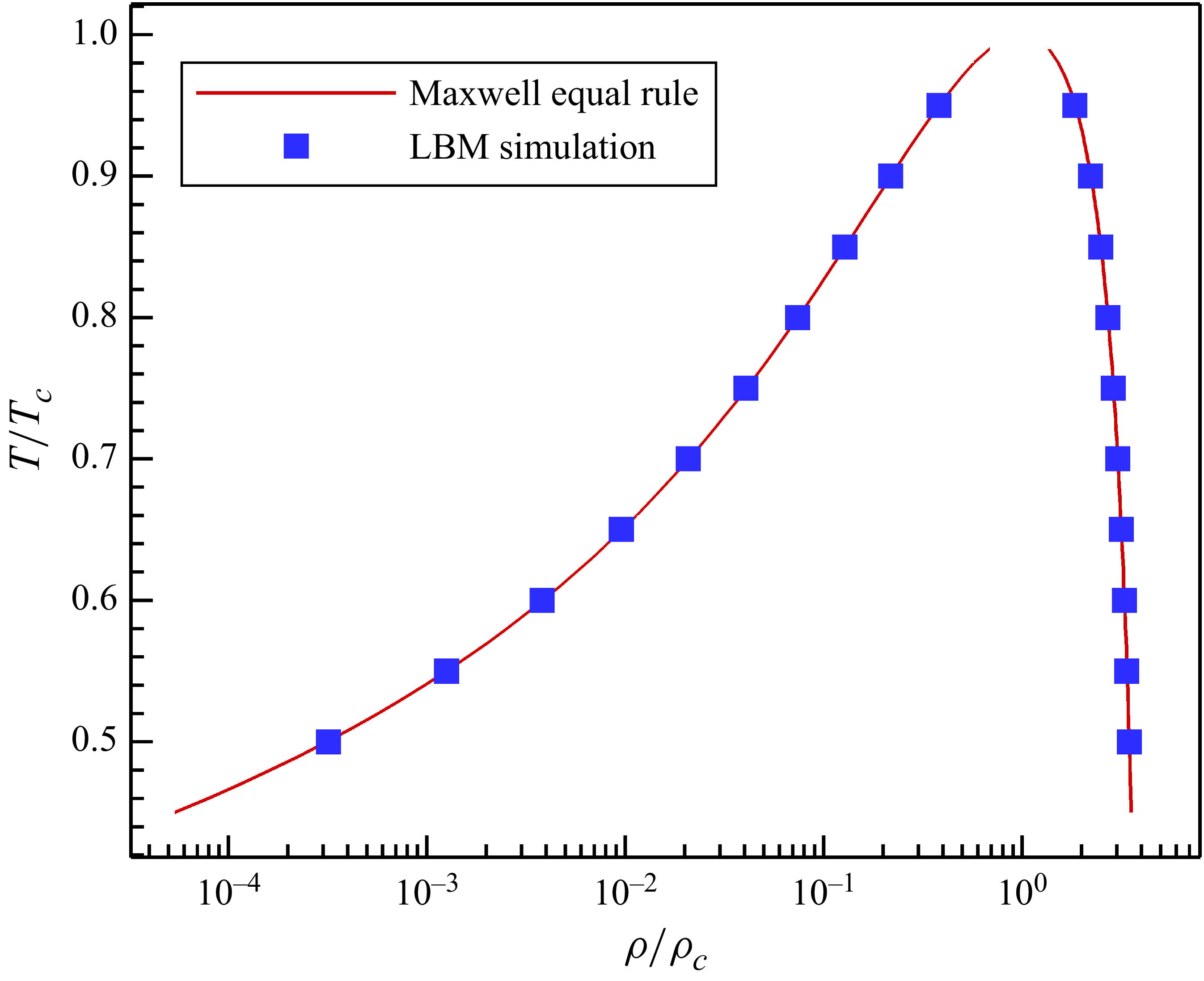
First, we validate the model by comparing the liquid–vapour density ratios with theoretical values obtained by the Maxwell equal area rule, to ensure thermodynamic consistency. The simulation set-up is very simple, i.e. a two-dimensional flat liquid–vapour interface. The selected temperature ratio ranges from
 $T/T_c=0.5$
to
 $0.95$
, with the corresponding liquid–vapour density ratio from
 $11\,073$
to
 $4.86$
. The comparison is shown in figure 2, where the liquid and vapour densities are normalised by dividing the critical density
 $\rho _c=1/{3.95b}=2.658$
(
 $b=2/21$
is the parameter in (2.24)). With the tuneable parameter
 $\lambda =-0.319$
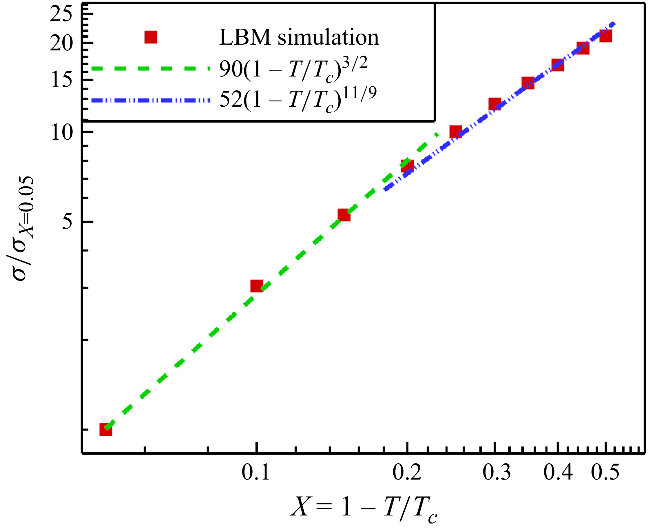
, very good agreement is obtained between the current LBM simulations and the Maxwell equal area rule, indicating thermodynamic consistency is accurately conserved with a wide range of density and temperature ratios. The thermodynamic consistency of current model is further validated following Hosseini et al. (Reference Hosseini, Dorschner and Karlin2022, Reference Hosseini, Dorschner and Karlin2023). As shown in Appendix B, the model works equally well for different non-ideal equations of state, and the scaling relations between surface tension/interface thickness and temperature agree well with theoretical relations.
Comparison of normalised liquid/vapour densities between current LBM simulations and Maxwell equal area rule at different temperature ratios.

Afterwards, we model a two-dimensional single droplet suspended in vapour without the consideration of gravity. The simulation domain is set as
 $240\times 240$
squares of grids, and the droplet radius is
 $50$
grids. The kinematic viscosity for both liquid and vapour are set as
 $\nu = 1/6$
. The four boundaries are set as periodic. The obtained droplet profile is shown in figure 3(a), while the corresponding velocity contour is given in figure 3(b). We observe that the maximum spurious current at the liquid–vapour phase is less that
 $0.004$
, a small value whose influence is negligible in the modelling of two-phase flow.
An LBM simulation of single droplet suspended in vapour. (a) Density contour. (b) Spurious current.

The calculation of
 $({{3G}}/{{2\rho }}) {\psi ^2}$
in (2.39) for both liquid and vapour phases under different temperature ratios
 $T/T_c$
.

In order to validate the model of surface tension adjustment, we vary the parameter
 $\kappa$
in (2.39). As shown in figure 4(a), with
 $\kappa$
increasing from −3 to 3.45, the surface tension ratio
 ${{{\sigma _\kappa }}}/{{{\sigma _{\kappa = 0}}}}$
decreases linearly from around 2 times to 1 %. The approximated linear function is obtained as
 ${{{\sigma _\kappa }}}/{{{\sigma _{\kappa = 0}}}} = 1.029-0.295\kappa$
. Here, we compare the obtained linear function with the theoretically derived (2.39). In (2.39), the parameter
 $\lambda$
is set as
 $\lambda =-0.319$
as mentioned above. For the value of
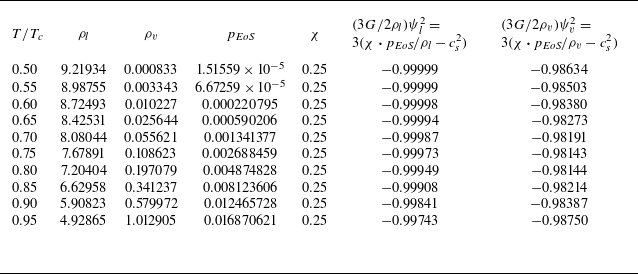
 $({{3G}}/{{2\rho }}) {\psi ^2}$
, we calculate it by
 $\chi \boldsymbol{\cdot }{P_{\textit{EoS}}} = \rho c_s^2 + ({{G{c^2}}}/{2}) {\psi ^2}$
, i.e.
 $({{3G}}/{{2\rho }}) {\psi ^2} = 3({\chi \boldsymbol{\cdot }p_{\textit{EoS}}}/\rho - c_s^2)$
. For the calculation of
 ${p_{\textit{EoS}}}/\rho$
, as shown in table 1,
 $({{3G}}/{{2\rho }}) {\psi ^2}$
under different temperature ratios from
 $T/T_c=0.50$
to
 $0.95$
remains basically a constant for both liquid (
 ${p_{EoS,l}}/{\rho _l}$
) and vapour (
 ${p_{EoS,v}}/{\rho _v}$
) properties. The maximum difference is less than 1.8 %. In this work, we calculate
 $({{3G}}/{{2\rho }}){\psi ^2}$
simply by taking the average value of it using the data in table 1, which is
 ${(({{3G}}/{{2\rho }}){\psi ^2})_{ave}} = - 0.9915$
. And thus (2.39) is simplified as
 ${{{\sigma _\kappa }}}/{{{\sigma _{\kappa = 0}}}} = 1-0.290\kappa$
, which is almost identical to our obtained function of
 ${{{\sigma _\kappa }}}/{{{\sigma _{\kappa = 0}}}} = 1.029-0.295\kappa$
in figure 4(a). The excellent agreement indicates remarkable high accuracy of current proposed model. We also note that, by choosing
 $\lambda =-0.319$
and
 $({{3G}}/{{2\rho }}){\psi ^2}$
calculated as
 $-0.9915$
, the parameter to adjust thermodynamic consistency is calculated as
 $\varepsilon = - 2(\lambda + {{G{\psi ^2}}}/{\rho }) = 1.96$
, a value between 1 and 2 agrees with the analysis by Li et al. (Reference Li, Luo and Li2012). We emphasise that, the good agreement between our LBM simulation results and the theoretical equation benefits from the consideration of the error terms (2.25). If we do not consider the error term, the original theoretical equation of surface tension adjustment is written as
 $ {{{\sigma _\kappa }}}/{{{\sigma _{\kappa = 0}}}} = {{1 - \lambda - ({{2\kappa }}/{3}}})/{{1 - \lambda }}$
instead (Wang et al. Reference Wang, Fei and Luo2022). As shown in figure 4(a), the original equation significantly deviates from the current theoretical equation (2.39) and simulation results, indicating the importance of current improvement in considering the error term. An important issue that determines whether the surface tension adjustment model is practical, is the variation of maximum spurious current with the change of surface tension. As shown in figure 4(b), when the surface tension ratio varies around 200 times, the maximum spurious current
 $|V|_{max}$
only increases from 0.002 to 0.0044 by around 2 times. The maximum spurious current is still low enough, and its influence on the two-phase dynamics can still be neglected.
(a) Comparison of surface tension adjustment between current LBM simulation and our theoretical equation (2.39) considering error term and original equation by Wang et al. (Reference Wang, Fei and Luo2022). (b) The variation of maximum spurious current under different
 $\kappa$
.

Finally, in this subsection, we try to realise different surface wettabilities using (2.40) in § 2.4. Three different contact angles spanning a wide range from
 $\theta =31.6^\circ$
at
 $\varphi =1.4$
to
 $\theta =89.1^\circ$
at
 $\varphi =1.0$
and
 $\theta =150.8^\circ$
at
 $\Delta \rho =40\rho _v$
are realised, as shown in figure 5. The spurious current of the three cases is also illustrated in figure 5, where we clearly observe that the spurious current is higher around the liquid–vapour–solid triple line for
 $\theta =31.6^\circ$
and
 $\theta =150.8^\circ$
. Despite that, the maximum spurious current is around 0.0053, which is still small enough to be neglected in the study of droplet dynamics in this paper.
The realisation of three contact angles using (2.40). Panels show (a)
 $\theta =31.6^\circ$
at
 $\varphi =1.4$
, (b)
 $\theta =89.1^\circ$
at
 $\varphi =1.0$
, (c)
 $\theta =150.8^\circ$
at
 $\Delta \rho =40\rho _v$
. The white curves indicate the droplet profiles while the contours represent the spurious current.

3.2. Droplet splashing on thin liquid film
In this subsection, we study the two-dimensional droplet impact on a thin liquid film with various Reynolds and Weber numbers. Droplet impact on a liquid film and the resultant splashing are studied both experimentally (Mundo, Sommerfeld & Tropea Reference Mundo, Sommerfeld and Tropea1995; Cossali et al. Reference Cossali, Marengo, Coghe and Zhdanov2004) and numerically (Li et al. Reference Li, Luo and Li2013; Qin et al. Reference Qin, Moqaddam, Ali, Qinjun and Carmeliet2018) in the literature. In terms of numerical modelling, the achievement of high Reynolds and Weber numbers is a big challenge. Li et al. (Reference Li, Luo and Li2013) proposed an improved MRT-LBM to realise Reynolds and Weber numbers of
 ${\textit{Re}}=1000, {\textit{We}}=103$
at a high liquid–vapour density ratio of
 $\rho _l/\rho _v=1000$
. Later, Qin et al. (Reference Qin, Moqaddam, Ali, Qinjun and Carmeliet2018) combined EMRT-LBM with a multi-layer pseudopotential model, and realised higher Reynolds and Weber numbers of
 ${\textit{Re}}=5000, {\textit{We}}=220$
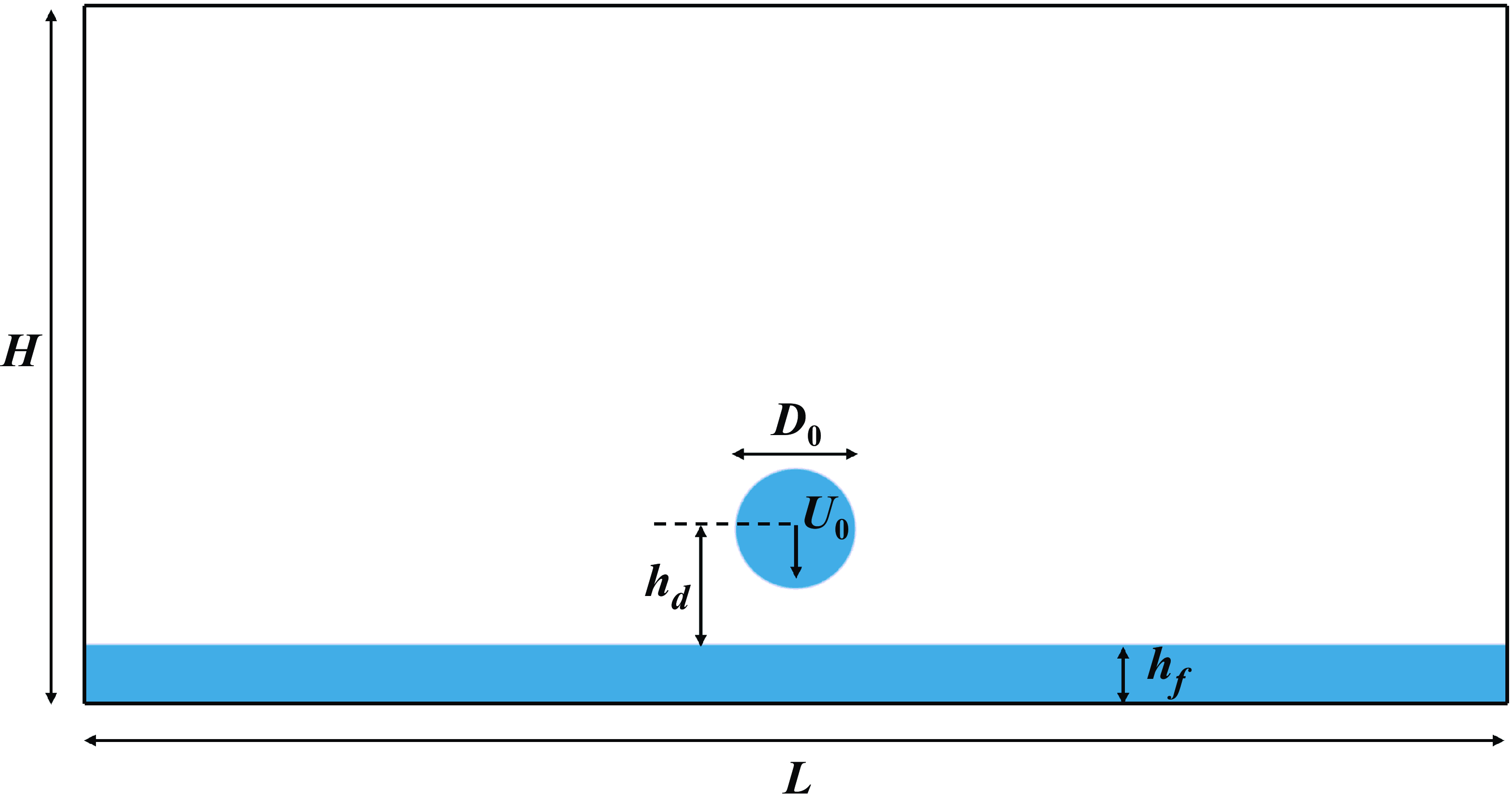
. In this subsection, we further extend the modelled range of Weber number, to investigate how a high Weber number influences the splashing dynamics. The simulation set-up is shown in figure 6, with a two-dimensional domain size of
 $L=2400$
and
 $H=1200$
grids. The top and bottom boundaries are no-slip walls, while the left and right sides are periodic. The film thickness is
 $h_f=100$
grids, and a droplet of diameter
 $D_0=200$
grids is placed above the film with a height of
 $h_d=120$
grids. The droplet initial velocity is
 $U_0=0.12$
in all simulation cases in this subsection. The vapour viscosity is set as
 $\nu _v=1/6$
, while the liquid viscosity is determined by the Reynolds number. The parameter
 $\kappa$
is set according to the linear relation in figure 4(a) to realise different Weber numbers. In this paper, Reynolds and Weber numbers are defined as
 ${\textit{Re}}=U_0D_0/\nu _l, {\textit{We}}=\rho _l*U_0^2D_0/\sigma$
. We conduct three simulations with
 ${\textit{Re}}=220, {\textit{We}}=220$
,
 ${\textit{Re}}=5000, {\textit{We}}=220$
and
 ${\textit{Re}}=5000, {\textit{We}}=5000$
.
Simulation set-up of two-dimensional droplet impact on a thin liquid film.

For the first case of
 ${\textit{Re}}=220, {\textit{We}}=220$
, the droplet impact and spreading dynamics are shown in figure 7(a). The dimensionless time is defined as
 $t^*=U_0t/D_0$
, where
 $t=0$
is the time frame when the droplet reaches the liquid film. After the droplet starts to merge with the liquid film at
 $t^*=0.24$
, a thin liquid sheet is emitted at
 $t^*=0.96$
. The liquid sheets keeps growing with time to form a ”crown” shape, while the droplet top arc gradually becomes flatter (at
 $t^*=3.6$
). No droplet splashing is observed since both the Reynolds and Weber numbers are relatively low. At a much higher Reynolds number of
 ${\textit{Re}}=5000$
as shown in figure 7(b), the droplet starts to splash at the tip of the liquid sheets at
 $t^*=1.68$
. More secondary droplets are observed with time as shown at
 $t^*=3.6$
. The result at
 ${\textit{Re}}=5000, {\textit{We}}=220$
is consistent with that in Qin et al. (Reference Qin, Moqaddam, Ali, Qinjun and Carmeliet2018). If we further increase the Weber number to a much higher value of
 ${\textit{We}}=5000$
while maintaining the Reynolds number of
 ${\textit{Re}}=5000$
, we observe the liquid sheets are much thinner and higher, as shown in figure 7(c). Moreover, more secondary droplets occur during splashing (at
 $t^*=3.6$
), and the secondary droplets are much smaller. The results are physical since the liquid viscosity and surface tension are smaller in figure 7(b)–(c) than in figure 7(a), making the liquid much easier to deform and breakup. The qualitative trend of droplet splashing also follows the theoretical study by Mundo et al. (Reference Mundo, Sommerfeld and Tropea1995), i.e. strong splashing occurs with the increase of the Sommerfeld parameter
 $S=We^{1/2}Re^{1/4}.$
Compared with the modelling of droplet impact on a liquid film at
 ${\textit{We}}=311, 328$
in Wu et al. (Reference Wu, Chen and Chen2020) and Zhang et al. (Reference Zhang2024), the Weber number of
 ${\textit{We}}=5000$
realised by our modelling is approximately 15 times higher.
Droplet impact on a liquid film at different Reynolds (Re) and Weber (We) numbers (corresponding to supplementary movies SM1–3). Panels show (a)
 ${\textit{Re}}=220, {\textit{We}}=220$
, (b)
 ${\textit{Re}}=5000, {\textit{We}}=220$
, (c)
 ${\textit{Re}}=5000, {\textit{We}}=5000$
. The dimensionless time is defined as
 $t^*=U_0t/D_0$
.

To better analyse the spreading of the droplet radius, the growing of the liquid sheet, as well as the breakup of the secondary droplets, we plotted the velocity vector (left half) and contour (right half, normalised by the initial impact velocity
 $U_0$
) of the case
 ${\textit{Re}}=5000, {\textit{We}}=5000$
at
 $t^*=2.40$
, as shown in figure 8. We clearly see the main flow is mainly in the liquid sheets and the thin film between them. The flow in the thin film in between is towards the liquid sheets, showing the spreading behaviour. For the liquid sheets, they grow in the directions of both radius and height, but mainly in the height direction. The velocity magnitude is getting higher with the liquid sheet becoming thinner. When the liquid sheet is thin enough, it breaks up into secondary droplets that fly away from the thin liquid sheets with a high speed.
Velocity vector (left half) and distribution (right half) of the liquid film and splashing droplet at the dimensionless impact time of
 $t^*=U_0t/D_0=2.40$
at
 ${\textit{Re}}=5000, {\textit{We}}=5000$
. For a clear view, only
 $1/10$
of the vectors are shown.

During the observation of the secondary droplets after splashing, we found the smaller ones tend to disappear with time (figure 7
c). These behaviours are actually the shrinkage effects studied by Yue, Zhou & Feng (Reference Yue, Zhou and Feng2007), where droplets or bubbles below a critical size tend to shrink spontaneously. This effect is an inherent feature of diffuse interface numerical models, driven by the redistribution of interface and bulk energies to minimise the total energy of the entire system. The critical size is found to increase with system size and interface thickness for suspended droplets/bubbles (Yue et al. Reference Yue, Zhou and Feng2007; Zheng et al. Reference Zheng, Lee, Guo and Rumschitzki2014). In our cases, interface thickness is around 6–7 grids (normally 5–6 grids for the low liquid–vapour density ratio case), making the critical size a little higher. The system size of
 $2400\times 1200$
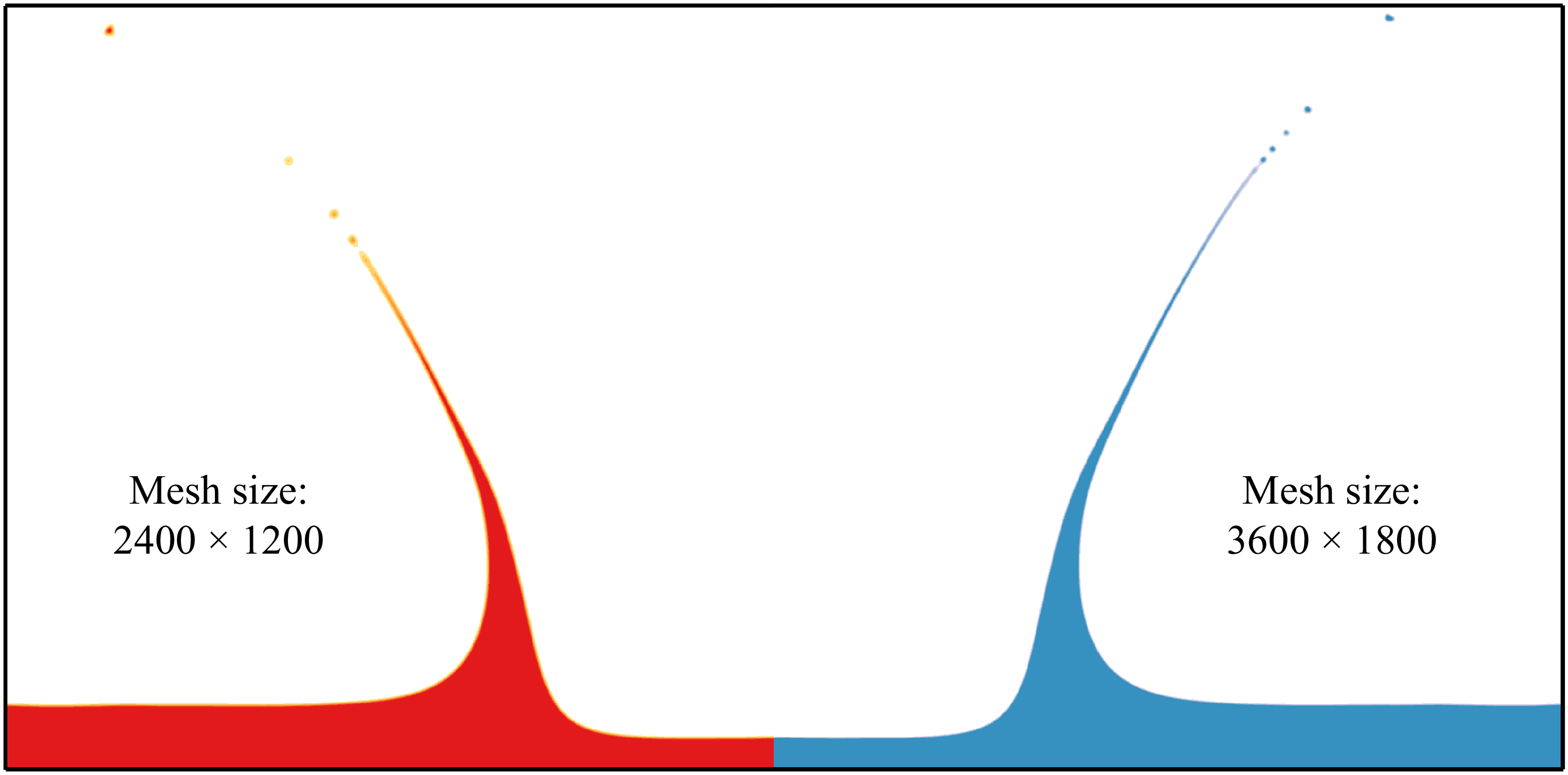
squares of grids is also very large, so that the secondary droplets are more likely to be unstable and finally disappear. We also conducted a simulation at a larger system size of
 $3600\times 1800$
squares of grids, to compare with the results of system size
 $2400\times 1200$
squares of grids. The comparison at the time frame of
 $t^*=3.72$
for
 ${\textit{Re}}=5000, {\textit{We}}=5000$
is shown in figure 9. We can see they are very similar, and the only difference may lie in the height of the thin liquid sheet. The thin liquid sheet of larger system size is higher, since the ratio of liquid–vapour interface thickness to the sheet thickness is smaller, making it more stable.
Comparison of splashing phenomena at
 ${\textit{Re}}=5000, {\textit{We}}=5000$
at different mesh sizes of
 $2400 \times 1200$
(left half, red) and (b)
 $3600 \times 1800$
(right half, blue) squares of grids at
 $t^*=3.72$
.

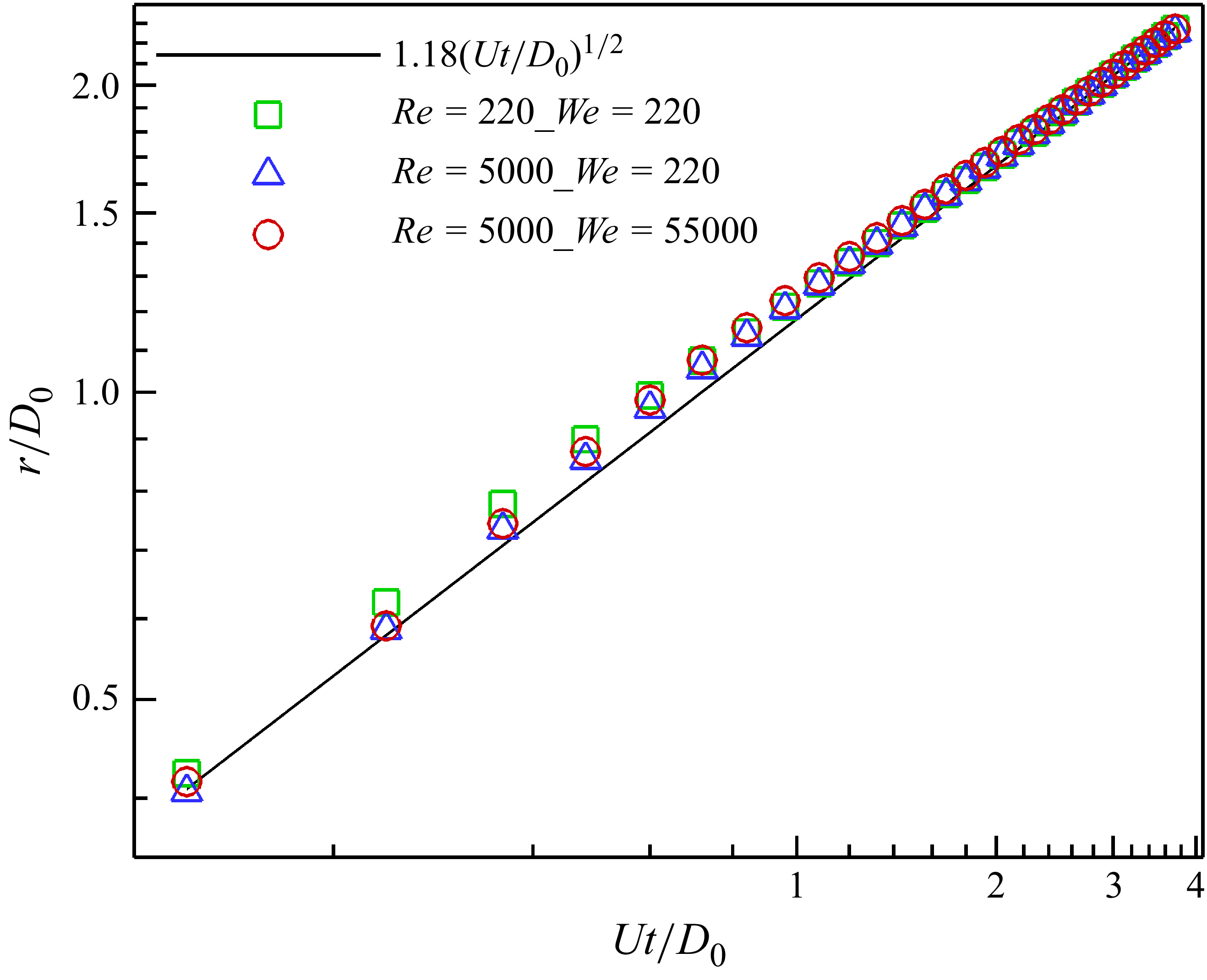
Finally in this subsection, we compare the spreading radius of the droplet during the impact process. The plot of normalised spreading radius
 $r/D_0$
versus the dimensionless time
 $t^*=U_0t/D_0$
for different cases is given in figure 10. Theoretically, the spreading radius follows the square root of time law (Josserand & Zaleski Reference Josserand and Zaleski2003)
 \begin{align} r/{D_0} = C\sqrt {{U_0}t/{D_0}} , \end{align}
where
 $C$
is a coefficient found to be larger than 1.1 in previous two-dimensional modelling results (Li et al. Reference Li, Luo and Li2013; Qin et al. Reference Qin, Moqaddam, Ali, Qinjun and Carmeliet2018). In figure 10, we can see that the simulation results at different Reynolds and Weber numbers agree well with the theoretical relation with
 $C=1.18$
, indicating the simulations agree well with the empirical equation.
Normalised spreading radius
 $r/D_0$
as a function of dimensionless time
 $t^*=U_0t/D_0$
. Symbols: LBM simulations at different Reynolds and Weber numbers of (
 ${\textit{Re}}=220, {\textit{We}}=220$
), (
 ${\textit{We}}=5000, {\textit{We}}=220$
) and (
 ${\textit{Re}}=5000, {\textit{We}}=5000$
). Line: empirical equation of square root of time law (Josserand & Zaleski Reference Josserand and Zaleski2003).

3.3. Droplet impact and splashing on flat surfaces
3.3.1. Impact and splashing phenomena at different Re and We
To further illustrate the model capability, we study droplet impact on a flat surface with various Reynolds and Weber numbers, considering different surface wettabilities. We note that, for a three-dimensional flat interface, the equilibrium liquid–vapour density ratio is around
 ${\rho _l}/{\rho _v} \approx 1052$
at
 $T/{T_c} = 0.59$
. However, for all the three-dimensional simulations of droplet impact, due to curvature and variation of surface tension, both liquid and vapour densities vary to some extent, leading to the actual density ratio being in the range of
 ${\rho _l}/{\rho _v} \in (641,989)$
. For the first case, we model droplet impact on a neutral surface with equilibrium contact angle
 $\theta =90^\circ$
. The droplet impact velocity is 1.0 ms−1, and the diameter is 2.28
 $\rm mm$
, leading to a Weber number of
 ${\textit{We}}=31.5$
(Yokoi et al. Reference Yokoi, Vadillo, Hinch and Hutchings2009). In our simulation, we use a droplet with diameter of
 $D_0=120$
grids, while the initial impact velocity is set as
 $U_0=0.079$
. The three-dimensional domain size is
 $480\times 480\times 360$
cubic of grids. To realise the same Weber number as in the experiment, we set surface tension as
 $\sigma =0.2086$
. To compare the droplet configuration at different time frames, we convert simulation time to physical time by ensuring the same dimensionless time, i.e.
 $t^* = {U_{0}}{t}/{D_{0}}$
. As shown in figure 11(a), the simulated droplet configurations agree well with the experimental ones at different time frames from
 $0$
to
 $30\,\rm ms$
. During the impact process, the droplet first expands (
 $2\,\rm ms$
) and reaches the maximum spreading diameter (
 $4\,\rm ms$
). Afterwards, the droplet contact diameter recedes while the droplet height increases and reaches maximum (
 $4{-}$
 $15\,\rm ms$
). At around
 $30\,\rm ms$
, the droplet reaches a quasi-static condition. Quantitatively, we recorded the evolution of spreading diameter. As shown in figure 11(b), the LBM simulation result generally agrees well with the experiment. A small difference between
 $22$
and
 $30\,\rm ms$
mainly originates from the fact that, in the experiment, the droplet contact line moves at a dynamic contact angle. As investigated by Yokoi et al. (Reference Yokoi, Vadillo, Hinch and Hutchings2009), the contact angle varies from around
 $\theta =50^\circ$
to
 $\theta =120^\circ$
, showing a dependence on the contact line velocity. By implementing the dynamic contact angle model in the volume of fluid method, Yokoi et al. (Reference Yokoi, Vadillo, Hinch and Hutchings2009) successfully reproduced the droplet dynamics, showing good agreement with experimental results. Very recently, Zhu et al. (Reference Zhu, Wang, Dai, Wang and Wang2025) implemented the dynamic contact angle in LBM for a droplet impact study. Since our current work mainly focuses on droplet impact and splashing at high Reynolds and Weber numbers, we skip the implementation of the dynamic contact angle model here, but we will incorporate it in our model in the future for a more comprehensive study of droplet impact and splashing.
Comparison of droplet impact on neutral flat surface (
 $\theta =90^\circ$
) at
 ${\textit{We}}=31.5$
between experimental (grey, (Yokoi et al. Reference Yokoi, Vadillo, Hinch and Hutchings2009)) and current LBM simulation (blue, corresponding to supplementary movie SM4)) results. (a) Droplet configuration at different time frames. (b) Evolution of droplet contact diameter with time.

The above simulation models droplet impact on a neutral surface (
 $\theta =90^\circ$
). Study of droplet impact on superhydrophobic surfaces has become very popular, since contact time and contact diameter could be reduced very effectively. In this case, we model droplet impact on a superhydrophobic surface with contact angle of
 $\theta =157^\circ$
. In the experiment (Bird et al. Reference Bird, Dhiman, Kwon and Varanasi2013), the droplet impact velocity is
 $1.2\,\rm m\,s^{-1}$
, and the initial diameter is
 $2.66\,\rm mm$
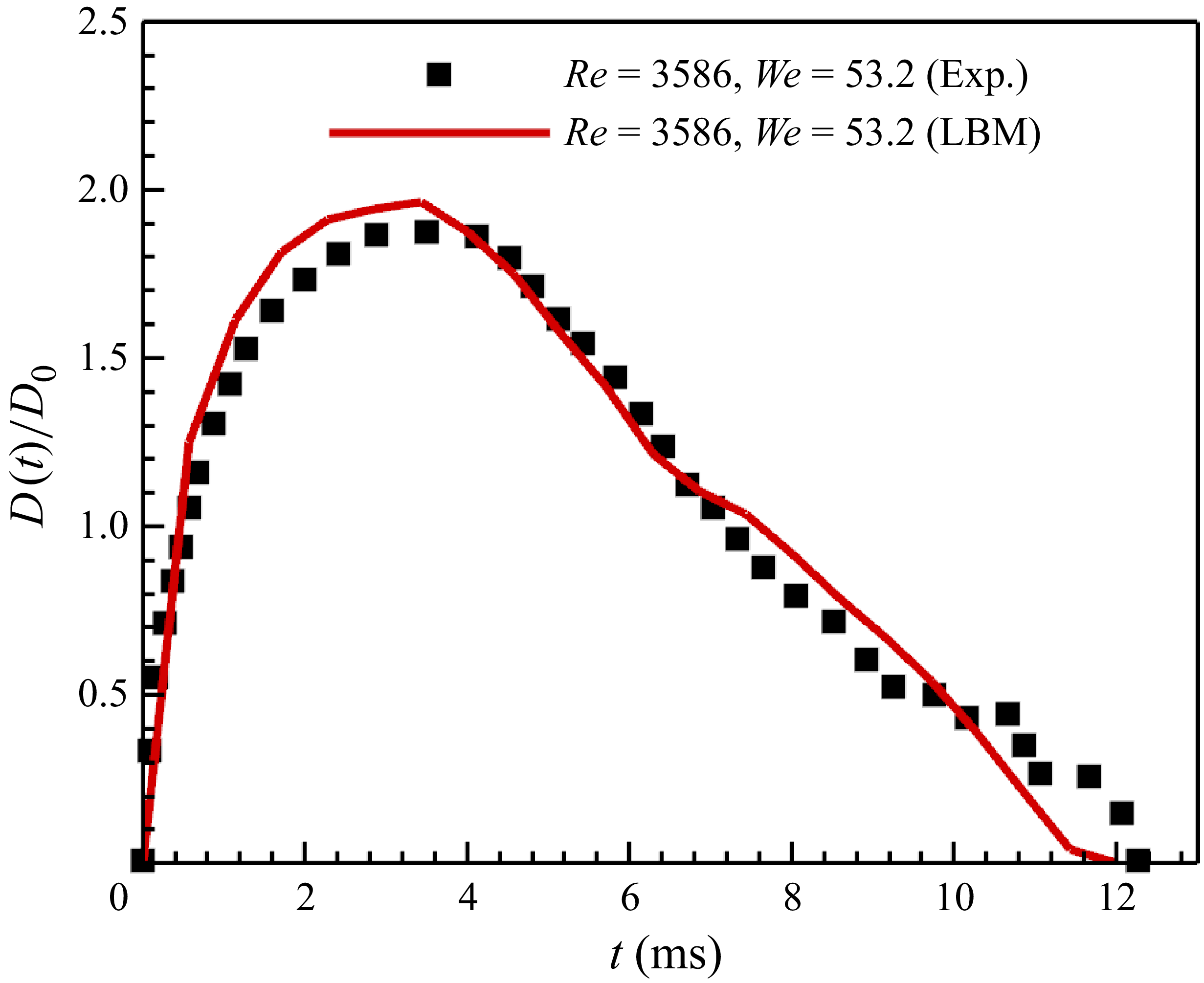
, resulting in relatively higher Reynolds and Weber numbers of
 ${\textit{Re}}=3586, {\textit{We}}=53.2$
. In the current simulation, the droplet diameter is also set as
 $D_0=120$
grids, while the initial impact velocity is set as
 $U_0=0.12$
. The liquid viscosity and surface tension are set as
 $\nu _l=0.004$
and
 $\sigma =0.2858$
, respectively. The three-dimensional domain size is
 $360\times 360\times 480$
cubic of grids. With this set-up, the droplet impact process is obtained as shown in figure 12. At around
 $2.8\,\rm ms$
, the droplet reaches its maximum diameter and then starts to recede (
 $4.6\,\rm ms$
). At around
 $7.5\,\rm ms$
, the droplet forms a mountain-like shape and continues bouncing until it departs solid surface at
 $12.4\,\rm ms$
. Due to high Reynolds and Weber numbers, the droplet splashes into a main droplet and a secondary droplet at top. The simulation droplet dynamic process agrees very well with the experimental result, as compared in figure 12. For droplet contact diameter evolution, as shown in figure 13, good agreement is also obtained between modelling and experimental result. The above two simulations of droplet impact on flat surfaces with different surface wettabilities and Reynolds/Weber numbers show that the current developed LBM is very accurate in modelling complex two-phase dynamics.
Comparison of droplet impact on superhydrophobic flat surface (
 $\theta =157^\circ$
) at
 ${\textit{Re}}=3586, {\textit{We}}=53.2$
between experimental (grey, Bird et al. Reference Bird, Dhiman, Kwon and Varanasi2013) and current LBM simulation (blue, corresponding to supplementary movie SM5) results.

Comparison of droplet contact diameter on flat surface at
 ${\textit{Re}}=3586, {\textit{We}}=53.2$
between experimental Bird et al. (Reference Bird, Dhiman, Kwon and Varanasi2013) and current LBM simulation result.

The above simulations show the current model works well for modelling flows with relatively low Weber numbers. To further illustrate the capability of current model, we model droplet splashing on a superhydrophobic solid surface at very high Reynolds and Weber numbers of
 ${\textit{Re}}=15\,200, {\textit{We}}=1020$
, respectively. The droplet diameter is also set as
 $D_0=160$
grids, with the initial impact velocity still set as
 $U_0=0.12$
. The liquid viscosity and surface tension are set as
 $\nu _l=0.00126$
and
 $\sigma =0.01988$
, respectively, in order to achieve high
 ${\textit{Re}}$
and
 ${\textit{We}}$
. The liquid–gas dynamic viscosity ratio is set as
 $\mu _l/\mu _v=16.0$
. The three-dimensional domain size is
 $960\times 960\times 300$
cubic of grids. The evolution of droplet configuration is shown in figure 14(a). At non-dimensional time
 $t^*=1.26$
, the droplet spreads after contact with the solid surface. At the edge of the spreading film, we observe some instability. Afterwards, the instability gradually exaggerates, until at
 $t^*=2.52$
the fingering structures occur with slight splashing to form several secondary droplets (Zhang et al. Reference Zhang, Zhang, Yi, He, Niu and Hao2021b
). With spreading, the fingers continuously grow to be longer. After reaching the maximum spreading at approximately
 $t^*=3.77$
, the droplet starts to recede, which pulls back the fingers and produce more intensive splashing (at
 $t^*=5.03$
and 5.97). From figure 14(a) we can see that the complex droplet splashings on a flat surface at high
 ${\textit{Re}}$
and
 ${\textit{We}}$
are modelled physically, i.e. the receding splashing with finger structures is correctly reproduced. We note that, in the work of Yang & Qin (Reference Yang and Qin2024), they modelled droplet splashing on a superhydrophobic flat surface with fingering phenomenon, but at a small liquid–vapour density ratio of 145 with relatively low Reynolds and Weber numbers of
 ${\textit{Re}}=8000$
and
 ${\textit{We}}=321$
(figure 14
b). In the work of Xu et al. (Reference Xu, Tian, Zhu and Zhao2024), they modelled droplet splashing with high Reynolds and Weber numbers of
 ${\textit{Re}}=18000$
and
 ${\textit{We}}=140$
,
 ${\textit{We}}=1280$
, respectively, but they failed to capture the fingering phenomenon. Instead, some liquid rings (figure 14
c) occur before they breakup into secondary droplets. According to our best knowledge, in the framework of pseudopotential two-phase LBM, it is the first time we physically modelled the fingering phenomenon of droplet impact and splashing at such high
 ${\textit{Re}}$
and
 ${\textit{We}}$
numbers.
(a) Droplet splashing at different non-dimensional times
 $t^*=U_0t/D_0$
after impact on flat surface at
 ${\textit{Re}}=15\,200, {\textit{We}}=1020$
with current developed LBM (corresponding to supplementary movies SM6). (b) Droplet splashing at a small liquid–vapour density ratio of 145 with
 ${\textit{Re}}=8000$
and
 ${\textit{We}}=321$
(Yang & Qin Reference Yang and Qin2024). (c-d) Droplet splashing at
 ${\textit{Re}}=18\,000$
and
 ${\textit{We}}=140$
and
 ${\textit{We}}=1280$
, respectively (Xu et al. Reference Xu, Tian, Zhu and Zhao2024).

3.3.2. Influence of surface wettability and liquid–gas viscosity ratio on splashing
In this subsection, the influence of surface wettability and the liquid–gas viscosity ratio on the splashing dynamics is examined for
 ${\textit{Re}} = 15\,200$
and
 ${\textit{We}} = 1020$
, with all other simulation parameters identical to those in figure 14(a). The effect of wettability is investigated for contact angles in the range of
 $\theta = 30^\circ$
to
 $150^\circ$
, focusing on its role in the growth of interfacial instabilities and the onset of splashing. To quantify the peripheral instability, two characteristic spreading radii are introduced: the inner radius, representing the expansion of the bulk droplet, and the outer radius, representing the overall extent of the droplet, including interfacial fingers and secondary droplets (figure 15
a). The difference between these radii provides a direct measure of the degree of finger development or splashing. Representative three-dimensional and side views of the impact dynamics for various
 $\theta$
are presented in figure 15(b)–(f). The results show that increasing
 $\theta$
promotes instability growth. For
 $\theta \lt 90^\circ$
, splashing is suppressed by the strong adhesion to the hydrophilic surface. At
 $\theta = 120^\circ$
, pronounced splashing emerges at
 $t^* = 6.9$
, whereas on the superhydrophobic surface with
 $\theta = 150^\circ$
, more intense splashing is initiated earlier, at
 $t^* = 6.0$
. In the latter case, the high repellency of the surface facilitates the detachment of fingers and secondary droplets, as shown in figure 15(f).
(a) Illustration of inner and outer radii during droplet impact. (b)–(f) Three-dimensional and side views of representative droplet configurations at different contact angles.

To quantitatively assess the influence of contact angle on instability growth and splashing, we plot the temporal evolution of the normalised inner and outer droplet diameters in figure 16(a–e), where solid symbols denote the maximum spreading diameters. In all cases, the inner diameter reaches its maximum earlier than the outer diameter, and the time required to attain these maxima generally decreases with increasing contact angle. For
 $\theta = 30^\circ$
,
 $60^\circ$
and
 $90^\circ$
, the evolutions are similar: the maximum outer diameters occur at approximately
 $t^* = 6.9$
, and the inner diameters exhibit minimal reduction after attaining their peaks. In contrast, for hydrophobic surfaces with
 $\theta = 120^\circ$
and
 $150^\circ$
, the inner diameters reach their maxima rapidly and then recede at high rates, while the outer diameters continue to grow. This disparity leads to pronounced finger growth and subsequent splashing (highlighted by dashed lines in figure 16
d–e). A comparison of the maximum inner and outer diameters across contact angles is presented in figure 16(f). Both decrease approximately linearly with contact angle, owing to the reduced spreading capability of droplets on less wettable surfaces.
(a)–(e) The evolution of normalised droplet inner and outer diameters. (f) Comparison of maximum inner and outer diameters at different contact angles.

Another key parameter affecting the splashing dynamics is the liquid–gas viscosity ratio. In this study, the liquid viscosity is held constant while the gas viscosity is varied to produce different dynamic viscosity ratios of
 $\mu _l/\mu _v = 1$
,
 $4$
,
 $8$
,
 $12$
and
 $16$
. The contact angle is fixed at
 $\theta = 150^\circ$
. Representative droplet configurations at selected time frames are shown in figure 17. The case with
 $\mu _l/\mu _v = 16$
has already been presented in figure 14(a) and is therefore not repeated here. The results reveal that, in contrast to the fingering-type splashing driven by instability growth at
 $\mu _l/\mu _v = 8$
,
 $12$
and
 $20$
, markedly different phenomena occur at the low viscosity ratios of
 $\mu _l/\mu _v = 1$
and
 $4$
. In these cases, splashing arises without the formation of fingers and instead results from the breakup of a thin liquid rim at the droplet periphery. As shown in figure 17(a), the rim develops as a corona shape because the high gas viscosity retards the droplet’s radial spread over the solid surface. Consequently, the splashing observed in figure 17(a,b) is classified as corona splashing (Zhang et al. Reference Zhang, Zhang, Yi, He, Niu and Hao2021a
).
Droplet splashing at different liquid–gas viscosity ratios from
 $\mu _l/\mu _v=1$
to 12.

To quantify the spreading process, the evolutions of the inner and outer droplet diameters are plotted in figure 18(a–d). It is evident that corona splashing occurs much earlier than fingering splashing. For
 $\mu _l/\mu _v = 1$
(figure 18
a), fingering splashing follows the initial corona splashing. The detailed evolution is illustrated in figure 19: the corona-shaped rim grows at
 $t^* = 0.63$
and subsequently breaks up at
 $t^* = 1.9$
, initiating corona splashing. The main droplet then continues to spread, and peripheral instabilities develop (
 $t^* = 3.1$
), eventually giving rise to fingering splashing at
 $t^* = 4.4$
. The reduction in outer diameter after corona splashing in figure 18(a,b) is attributed to the disappearance of small secondary droplets. For
 $\mu _l/\mu _v = 4$
(figure 18
b), only corona splashing is observed. In this case, the gas viscosity is lower than for
 $\mu _l/\mu _v = 1$
, allowing the droplet to spread over the solid surface while forming a thick corona rim, as shown in the central-slice profiles in figure 18(f). However, the gas viscosity is still not sufficiently low to promote peripheral instability, thus preventing the onset of fingering splashing. At higher viscosity ratios of
 $\mu _l/\mu _v = 8$
and
 $12$
(figure 18
c,d), only fingering splashing occurs, consistent with the analysis in figure 16(e). In fact, the evolutions of inner and outer diameters become very alike once
 $\mu _l/\mu _v \geqslant 8$
(figure 18
e,f). The large disparity between inner and outer diameters for
 $\mu _l/\mu _v \leqslant 4$
reflects the distinct splashing mechanisms. At
 $\mu _l/\mu _v = 1$
(figure 18
e), the outer diameter is large while the inner diameter is small, because the high gas viscosity produces a thin corona rim prone to rapid breakup, which both decreases the inner diameter and increases the outer diameter. By contrast, for
 $\mu _l/\mu _v = 4$
, the smaller outer diameter and larger inner diameter correspond to the transitional regime from corona to fingering splashing, where the thick corona rim suppresses instability growth.
(a)–(d) The evolution of normalised droplet inner and outer diameters. (e) Comparison of maximum inner and outer diameters at different liquid–gas viscosity ratios. (f) Profiles of droplet central slice at different liquid–gas viscosity ratios.

Droplet configurations at different time frames at
 $\mu _l/\mu _v=1$
.

To summarise, we first reproduced the droplet impact and splashing on a flat surface at various
 ${\textit{Re}}$
and
 ${\textit{We}}$
, validating our simulations against existing experimental results. We then examined the effects of surface wettability and the liquid–gas viscosity ratio on splashing dynamics at high
 ${\textit{Re}}$
and
 ${\textit{We}}$
. The results show that hydrophobic surfaces facilitate the development of peripheral instabilities, leading to fingering splashing. At low liquid–gas viscosity ratios, corona splashing is dominant, transitioning to fingering splashing as the viscosity ratio increases.
3.4. Droplet impact on mesh structures
3.4.1. Impact and splashing phenomena at different Re and We
Droplet impacts on hydrophobic mesh structures have been studied both experimentally (Kumar et al. Reference Kumar, Tripathy, Nam, Lee and Sen2018; Kooij et al. Reference Kooij, Moqaddam, De Goede, Derome, Carmeliet, Shahidzadeh and Bonn2019) and numerically recently (Wang, Gao & Luo Reference Wang, Gao and Luo2020). The influences of mesh size and impact velocity on maximum spreading, contact time and distribution of secondary droplets, etc. are studied. However, for experimental results, the maximum Reynolds and Weber numbers studied are
 ${\textit{Re}}=8800$
and
 ${\textit{We}}=340$
. For modelling results, the maximum Reynolds and Weber numbers applied are around
 ${\textit{Re}}=1937$
and
 ${\textit{We}}=300$
, respectively, at maximum liquid–vapour density ratio of 500. We can see that, the modelled Reynolds number and density ratio are still far from real experimental set-ups. For both experimental and simulation studies, the Weber number is not high enough. In this subsection, we intend to study droplet impact on mesh structures with large ranges of Reynolds and Weber numbers, up to
 ${\textit{Re}}=15\,200$
and
 ${\textit{We}}=1020$
.
To validate our model for complex droplet impact on mesh structures, we compare modelling results with experimental results in (Kumar et al. Reference Kumar, Tripathy, Nam, Lee and Sen2018). The simulation set-ups are shown in figure 20. The domain size is around
 $480\times 480\times 720$
cubic of grids, with top and bottom are no-slip walls (not shown) and the lateral four sides periodic. The mesh structures made of fibres with a diameter of
 $r=15$
grids is placed at 210 grids from top of domain. The distance between fibre centres is
 $d=40$
grids. The droplet diameter is
 $D_0=120$
grids, and its initial centre is located at 90 grids from top boundary. For first 1000 iterations, the droplet is speeding up to fall with a gravity of
 $g=1.2\times 10^{-4}$
to reach mesh structure with a velocity of
 $U_0=0.12$
. Then gravity effect is eliminated to study the impact dynamics, since its influence is negligible (Wang et al. Reference Wang, Gao and Luo2020). In this paper, we mainly study the qualitative splashing dynamics and quantitative spreading diameter
 $D(t)$
as shown in figure 20.
(a) Simulation set-up of three-dimensional droplet impact on a mesh structure. (b) The mesh structures with different mesh sizes, i.e. ratios of pillar diameter and distance between pillar centres ranging from
 $2r/d=0.12$
to
 $0.75$
.

We first compare the results at
 ${\textit{Re}}=3520, {\textit{We}}=54.4$
. Similarly as in § 3.3, we compare the modelled droplet configuration at different time frames with experimental results by ensuring the same dimensionless time
 $t^*=U_0t/D_0$
in both lattice and physical units. As shown in figure 21, after droplet reaches mesh structure at
 $t=0.80 \, \rm ms$
, a part of liquid penetrates mesh structure through holes to form liquid sheets. At
 $t=1.60 \, \rm ms$
, penetration continues, together with spreading of the radius. At around
 $t=2.40 \, \rm ms$
, the spreading radius reaches its maximum, while penetration goes on and liquid sheets grow longer. Afterwards, droplet radius recedes, while liquid sheets still grow but become thinner at
 $t^*=3.20$
. Finally at
 $t^*=4.00$
, thin liquid sheets breakup into secondary droplets, which continuously flow downwards. The current LBM simulation results agree very well with experimental results at all time frames.
Comparison of droplet impact on mesh structure at
 ${\textit{Re}}=3520, {\textit{We}}=54.4$
between experimental (left half, (Kumar et al. Reference Kumar, Tripathy, Nam, Lee and Sen2018)) and current LBM simulation (right half, corresponding to supplementary movie SM7) results.

For case of higher Reynolds and Weber numbers at
 ${\textit{Re}}=6820, {\textit{We}}=204$
, the comparison is shown in figure 22. Compared with results at
 ${\textit{Re}}=3520, {\textit{We}}=54.4$
, the main difference here lies in the fact that the liquid sheets are getting thinner and longer. Moreover, the secondary droplets tend to be smaller. The reason is that, with higher Reynolds and Weber numbers, the inertial force is more dominant than the viscous force and capillary force. The qualitative trend here for droplet breakup is consistent with droplet splashing on a thin liquid film studied in § 3.2. Again, the LBM simulation results agree generally well with experimental results, indicating the current model is accurate in modelling the complex droplet dynamics through porous structures. We admit that, for both cases, there are still small discrepancies between current LBM simulations and experimental results. The reason mainly comes from the fact that mesh structure is not exactly the same as the knitted type in the experiments. Moreover, the exact impact location on mesh structure is not known, which also influences the splashing dynamics.
Comparison of droplet impact on mesh structure at
 ${\textit{Re}}=6820, {\textit{We}}=204$
between experimental (left half, (Kumar et al. Reference Kumar, Tripathy, Nam, Lee and Sen2018)) and current LBM simulation (right half, corresponding to supplementary movie SM8) results.

The above analyses are based on qualitative observation. Here we further compare spreading diameter in a quantitative view. The normalised diameter
 $D(t)/D_0$
versus time is shown in figure 23. For both cases, spreading diameter shows an increasing trend first, followed by a descending trend after reaching the maximum value. For case of
 ${\textit{Re}}=3520, {\textit{We}}=54.4$
, the maximum spreading diameter around
 $D(t)/D_0=1.7$
is reached at
 $t=2.40 \, \rm ms$
. For case of
 ${\textit{Re}}=6820, {\textit{We}}=204$
, the maximum spreading diameter is around
 $D(t)/D_0=1.87$
, approximately 10 % larger than that of
 ${\textit{Re}}=3520, {\textit{We}}=54.4$
. The time required to reach the maximum spreading is about
 $t=1.7 \, \rm ms$
, which is 30 % shorter than that of
 ${\textit{Re}}=3520, {\textit{We}}=54.4$
. For both two cases, the current LBM simulation results agree generally well with experimental results, further validating our model quantitatively.
Comparison of droplet spreading diameter after impact on mesh structure at
 ${\textit{Re}}=3520, {\textit{We}}=54.4$
and
 ${\textit{Re}}=6820, {\textit{We}}=204$
between experimental and current LBM simulation results. The spreading diameter of the droplet impact by LBM at
 ${\textit{Re}}=15\,200, {\textit{We}}=1020$
is also given.

After validation of the model for droplet splashing on mesh structures with moderate Reynolds and Weber numbers, we study more complex cases with much higher Reynolds and Weber numbers of
 ${\textit{Re}}=15\,200$
and
 ${\textit{We}}=1020$
, respectively. The comparison of simulation results between
 ${\textit{Re}}=6820, {\textit{We}}=204$
and
 ${\textit{Re}}=15\,200, {\textit{We}}=1020$
are shown in figure 24. From three representative states in figure 24(a–b), we can see the morphology of the droplets is very similar. The main differences lie in the liquid sheets being thinner/longer, while secondary droplets are smaller, consistent with results analysed above. For the droplet morphology above the mesh structure, from figure 24(c) we can see that it crushes into small clusters. Some clusters are inter-connected, while the others are isolated (at
 $t=0.896\,\rm ms$
) and may turn into secondary droplets splashing away from the main cluster. For the spreading diameter, we plotted it in figure 23 to compare with other simulation results. As expected, the maximum spreading diameter is around
 $D(t)/D_0=2.09$
, which is approximately 11.8 % larger than that of
 ${\textit{Re}}=6820, {\textit{We}}=204$
. The time required to reach the maximum diameter is reduced to nearly only half.
Comparison of droplet impact on mesh structure at (a)
 ${\textit{Re}}=6820, {\textit{We}}=204$
and (bc)
 ${\textit{Re}}=15\,200, {\textit{We}}=1020$
at different time frames (corresponding to supplementary movie SM9). Results in (ab) are side views and in (c) is a three-dimensional view.

A strong advantage of numerical modelling is the ability to analyse the flow field inside droplet and liquid sheets. As shown in figure 25, we can plot velocity vectors and contours (normalised by the impact velocity
 $U_0$
) during the splashing process. Figure 25(a) illustrates droplet and velocity vectors in space, where we see the velocity from the droplet top to bottom increases. The velocity at the droplet top part is small because it is hindered by the mesh structure. For penetrated liquid sheets, the velocity is much higher and leads to breakup of secondary droplets. Liquid sheets do not go straigh down, but at an angle towards the radius direction, as shown by the vectors. The central-plane cross-section in figure 25(b) shows the velocity in the liquid sheets and secondary droplets can be much higher than the initial droplet velocity (
 $0.12$
in lattice unit). This is because the droplet is squeezed into mesh holes, making the liquid sheets speed up. The qualitative analyses of the flow field further confirm the accuracy of the current multiphase model in studying the complex droplet dynamics.
(a) Droplet three-dimensional velocity contour with vector and (b) velocity profile at central slice during impact on mesh structure at
 $t=0.786$
ms at
 ${\textit{Re}}=15\,200, {\textit{We}}=1020$
.

3.4.2. Influence of mesh opening size on droplet spreading, penetration and splashing
In this subsection, we examine the effect of mesh size on droplet impact, penetration and the splashing dynamics at high Reynolds and Weber numbers (
 ${\textit{Re}} = 15\,200$
,
 ${\textit{We}} = 1020$
). As illustrated in figure 20(b), six mesh sizes are considered, characterised by the ratio of the solid pillar diameter (
 $2r$
) to the centre-to-centre spacing between pillars (
 $d$
), i.e. the solid ratios
 $2r/d = 0.12$
,
 $0.25$
,
 $0.38$
,
 $0.52$
,
 $0.63$
and
 $0.75$
.
In figure 26, representative droplet configurations during impact on different meshes are presented. At low solid ratios of
 $2r/d = 0.12$
and
 $0.25$
, the mesh openings are sufficiently large to permit droplet penetration. Spreading on the mesh surface before complete penetration is weak, with maximum spreading ratios below
 $1.4$
(figure 27
a). Penetration is also rapid, occurring within
 $0.9$
ms. For
 $2r/d = 0.12$
, the small pillar diameter causes minimal disruption of the droplet, and clear liquid pillars are not formed. As shown in figure 27(b), the normalised liquid pillar length
 $L_p(t)/D_0$
increases linearly at a high rate prior to full penetration, then decreases slightly at
 $t = 0.9\,\rm ms$
as the droplet contracts slightly once freed from the mesh constraint. This is followed by a slow elongation driven by inertia. For
 $2r/d = 0.25$
, distinct liquid pillars form during penetration. Owing to the large mesh openings, these pillars are relatively thick and can elongate considerably before breaking into secondary droplets. As shown in figure 27(b),
 $L_p(t)/D_0$
reaches
 $3.1$
at
 $2r/d = 0.25$
, the maximum among all cases. At a higher solid ratio of
 $2r/d = 0.38$
, figure 26(c) shows a larger spreading diameter, with a maximum spreading ratio of approximately
 $2.14$
(figure 27
a). The smaller mesh size prevents full penetration, and the resulting liquid pillars are thinner and more prone to breakup into small droplets. Consequently, the maximum
 $L_p(t)/D_0$
decreases to approximately
 $2.1$
, compared with
 $3.1$
for
 $2r/d = 0.25$
.
Representative droplet configurations (three-dimensional and side views) at different mesh sizes, i.e. the ratios of solid pillar diameter and distance between pillar centres ranging from
 $2r/d=0.12$
to
 $0.75$
.

The evolutions of (a) droplet spreading diameter and (b) penetrated liquid pillar length at different mesh sizes. The solid dots indicate maximum spreading or maximum penetration length before full penetration (if possible).

With further increase in solid ratio, liquid penetration becomes increasingly restricted. At
 $2r/d = 0.52$
(figure 26
d), only a small portion of the liquid penetrates the mesh, while the remaining volume spreads over the mesh surface. As shown in figure 27(a)–(b), the maximum spreading ratio rises to
 $2.93$
, whereas the normalised penetration length decreases to
 $1.16$
compared with smaller solid ratios. For even larger solid ratios (figure 26
e–f), penetration continues to diminish, while spreading increases. At
 $2r/d = 0.75$
(figure 26
f), penetration is nearly negligible, and the maximum spreading ratio reaches
 $3.43$
, the highest among all cases.
From the comparisons in figure 27(a), the droplet spreading diameter generally increases with time. For solid ratios of
 $2r/d = 0.12$
and
 $0.25$
, it rapidly drops to zero due to complete penetration. At higher solid ratios, complete penetration does not occur, yet the spreading diameter decreases slowly after reaching its maximum owing to droplet recession. Quantitatively, as shown in figure 28, the maximum spreading ratio
 $D_{\textit{max}}/D_0$
remains approximately constant for
 $2r/d \leqslant 0.25$
, then rises sharply up to
 $2r/d = 0.52$
, and continues to increase at a lower rate, peaking at
 $2r/d = 0.75$
with a value of
 $3.43$
, which is approximately 2.5 times that at
 $2r/d = 0.25$
. For liquid penetration, figure 27(b) shows that, at
 $2r/d = 0.12$
, the penetration length increases almost monotonically. At larger solid ratios, it increases generally before decreasing, and the duration of the increasing phase shortens as the solid ratio grows. Quantitatively, the maximum normalised penetration length before full penetration (if possible)
 $L_{p,\textit{max}}/D_0$
first rises and then decreases with increasing solid ratio, reaching a peak of
 $2.3$
at
 $2r/d = 0.25$
, approximately 9 times that at
 $2r/d = 0.75$
.
Maximum droplet spreading diameter
 $D_{max}/D_0$
and maximum liquid pillar penetration length before full penetration (if possible)
 $Lp_{max}/D_0$
at different mesh sizes.

To summarise, we first reproduced droplet impact and splashing on mesh structures at various
 ${\textit{Re}}$
and
 ${\textit{We}}$
, validating our simulations against existing experimental results. We then investigated the influence of mesh size on droplet impact, penetration and splashing dynamics. The results indicate that large openings promote liquid penetration, whereas small openings lead to greater spreading. As the solid ratio increases, the maximum spreading ratio rises monotonically but nonlinearly, while the maximum penetrated liquid pillar length first increases and then decreases.
4. Concluding remarks
In this paper, we proposed to couple the advanced EMRT (or KBC) LBM collision operator with a surface tension adjustment source term to model complex two-phase flows with wide ranges of liquid viscosity and surface tension. We first introduced the KBC model (Karlin et al. Reference Karlin, Bösch and Chikatamarla2014) with consideration of the external force to model two-phase flow. The influence of the force term on the entropic stabiliser is correctly taken into account. Then we applied the exact difference force scheme to incorporate the source term (Wang et al. Reference Wang, Fei and Luo2022) to adjust surface tension. Since the force scheme introduces a higher-order term, we theoretically derived the equation of how higher-order terms influence surface tension adjustment. Then we conducted simulations of a single droplet suspended in its vapour environment to validate the proposed coupling method of independently adjusting surface tension. We found that, with a high density ratio of around 1000, the surface tension tuneable range is over 200 times, while the maximum spurious current is maintained as low as 0.005 in lattice units (only accounting for around 5 % of the impact velocity, i.e.
 ${R_U} = {U_{spurious}}/{U_0} \in (4.2\,\% ,6.3\,\% )$
).
Then we applied the model to study droplet impact and splashing on a thin liquid film with three different combinations of Reynolds (Re) and Weber (We) numbers. With the increase of
 ${\textit{Re}}$
and/or
 ${\textit{We}}$
from 220 to 5000, splashing occurs and becomes more intensive with the formation of more secondary droplets. Liquid sheets also become thinner and taller. Droplet spreading radii are found to follow the empirical square root rule of time independently of
 ${\textit{Re}}$
or
 ${\textit{We}}$
. Afterwards, droplet impact and splashing on flat surfaces under different conditions are studied. Simulation results of droplet evolution configurations and spreading diameters agree well with experimental ones at
 ${\textit{We}}=31.5,\theta =90^\circ$
and
 ${\textit{We}}=53.2,\theta =157^\circ$
. At
 ${\textit{Re}}=15\,200, {\textit{We}}=1020$
at
 $\theta =150^\circ$
, splashing induced by the fingering phenomenon at the spreading film is physically modelled, for the first time at such high
 ${\textit{Re}}$
and
 ${\textit{We}}$
, in the framework of the pseudopotential LBM (
 ${\textit{We}}=321$
in Yang & Qin (Reference Yang and Qin2024)). The effects of surface wettability and the liquid–gas viscosity ratio on the splashing dynamics are further investigated at
 ${\textit{Re}}=15\,200, {\textit{We}}=1020$
. The results show that hydrophobic surfaces facilitate the development of peripheral instabilities, leading to fingering splashing. At low liquid–gas viscosity ratios, corona splashing is dominant, transitioning to fingering splashing as the viscosity ratio increases. Besides, droplet impact on hydrophobic mesh structures is studied at different combinations of
 ${\textit{Re}}$
and
 ${\textit{We}}$
. At
 ${\textit{Re}}=3520, {\textit{We}}=54.4$
, only several secondary droplets are observed after the primary droplet penetrates the mesh. At higher
 ${\textit{Re}}=6820, {\textit{We}}=204$
, liquid sheets become thinner after penetration, and more small secondary droplets occur. Both simulation results agree very well with experimental ones, including both the droplet deformation configuration and spreading diameter. Droplet impact at
 ${\textit{Re}}=15\,200, {\textit{We}}=1020$
(three times of those in (Wang et al. Reference Wang, Liu and Rajamuni2023)) is further simulated, showing that liquid sheets become thinner, longer while the spreading radius is larger and achieved earlier. The influence of mesh size on droplet spreading and penetration dynamics is also investigated. The results indicate that large openings promote liquid penetration, whereas small openings lead to greater spreading. As the solid ratio increases, the maximum spreading ratio rises monotonically but nonlinearly, while the maximum penetrated liquid pillar length first increases and then decreases.
The studies conducted in this work show the proposed coupled model is capable of modelling complex multiphase flow at a high density ratio of around 1000, low spurious current of around 0.005 in lattice unit, with wide ranges of liquid viscosity and surface tension (
 ${\textit{Re}}$
and
 ${\textit{We}}$
up to 15 200 and 5000). We note that, KBC LBM remains stable even on coarse grids due to a built-in implicit sub-grid model, leading to hyper-viscosity. Because of this, some of our three-dimensional simulations are not exactly direct numerical simulations, thus the effective
 ${\textit{Re}}$
may be lower than the reported values. The model is also shown to be capable of investigating the influences of different parameters (surface wettability, viscosity ratio, mesh size) on the spreading, penetration and splashing dynamics during droplet impact on flat and mesh structures. In the future, we would like to extend the model for more complex multiphase flows with non-isothermal phase change, such as evaporation and boiling, etc.
Supplementary movies
Supplementary movies are available at https://doi.org/10.1017/jfm.2025.11025.
Acknowledgements
National Natural Science Foundation of China (NSFC, No.12302337, No.12388101, No.52506104), Postdoctoral Special Project (K5002), Shaanxi Province Science Foundation for Youths (K1004), the 111 Project of China through Grant No.B17037, and the Central University Basic Research Fund of China (G2022KY05105) are acknowledged for the financial support. The Computing Center in Xi’an is acknowledged for the computational support.
Declaration of interests
The authors report no conflict of interest.
Appendix A. The construction of shear part
$\boldsymbol{s_i}$
in D3Q27 KBC model

For the D3Q27 LBM, the natural moments of different orders are constructed by
 \begin{align} \rho {M_{pqr}} = \sum \limits _{i = 0}^{Q - 1} {{f_i}c_{\textit{ix}}^pc_{\textit{iy}}^qc_{\textit{iz}}^r} ,p,q,r \in \{ 0,1,2\}. \end{align}
For convenience, we use the following linear combinations to represent the important natural moments to construct
 $s_i$
:
 \begin{align} \begin{array}{*{20}{c}} {T = {M_{200}} + {M_{020}} + {M_{002}},{N_{\textit{xz}}} = {M_{200}} - {M_{002}},{N_{\textit{yz}}} = {M_{020}} - {M_{002}},}\\ {{\varPi _{\textit{xy}}} = {M_{110}},{\varPi _{\textit{xz}}} = {M_{101}},{\varPi _{\textit{yz}}} = {M_{011}},{Q_{\textit{xyy}}} = {M_{120}},{Q_{xzz}} = {M_{102}},}\\ {{Q_{\textit{xxy}}} = {M_{210}},{Q_{\textit{yzz}}} = {M_{012}},{Q_{xxz}} = {M_{201}},{Q_{yyz}} = {M_{021}},{Q_{\textit{xyz}}} = {M_{111}}.} \end{array} \end{align}
With this set of natural moments, the shear part
 ${s_i} = {s_{({c_{\textit{ix}}},{c_{\textit{iy}}},{c_{\textit{iz}}})}}$
can be uniquely represented as Bösch et al. (Reference Bösch, Chikatamarla and Karlin2015)
 \begin{align} {s_{(0,0,0)}} &= - T,\nonumber\\ {s_{({c_{\textit{ix}}},0,0)}} &= \frac {1}{6}[2{N_{\textit{xz}}} - {N_{\textit{yz}}} + T - 3{c_{\textit{ix}}}({Q_{\textit{xyy}}} + {Q_{xzz}})],\nonumber\\ {s_{(0,{c_{\textit{iy}}},0)}} &= \frac {1}{6}[2{N_{\textit{yz}}} - {N_{\textit{xz}}} + T - 3{c_{\textit{iy}}}({Q_{\textit{xxy}}} + {Q_{\textit{yzz}}})],\nonumber\\ {s_{(0,0,{c_{\textit{iz}}})}} &= \frac {1}{6}[ - {N_{\textit{xz}}} - {N_{\textit{yz}}} + T - 3{c_{\textit{iz}}}({Q_{xxz}} + {Q_{yyz}})],\nonumber\\ {s_{({c_{\textit{ix}}},{c_{\textit{iy}}},0)}} &= \frac {1}{4}[{c_{\textit{ix}}}{c_{\textit{iy}}}{\varPi _{\textit{xy}}} + {c_{\textit{ix}}}{Q_{\textit{xyy}}} + {c_{\textit{iy}}}{Q_{\textit{xxy}}}],\nonumber\\ {s_{({c_{\textit{ix}}},0,{c_{\textit{iz}}})}} &= \frac {1}{4}[{c_{\textit{ix}}}{c_{\textit{iz}}}{\varPi _{\textit{xz}}} + {c_{\textit{ix}}}{Q_{xzz}} + {c_{\textit{iz}}}{Q_{xxz}}],\nonumber\\ {s_{(0,{c_{\textit{iy}}},{c_{\textit{iz}}})}} &= \frac {1}{4}[{c_{\textit{iy}}}{c_{\textit{iz}}}{\varPi _{\textit{yz}}} + {c_{\textit{iy}}}{Q_{\textit{yzz}}} + {c_{\textit{iz}}}{Q_{yyz}}],\nonumber\\ {s_{({c_{\textit{ix}}},{c_{\textit{iy}}},{c_{\textit{iz}}})}} &= \frac {1}{8}{c_{\textit{ix}}}{c_{\textit{iy}}}{c_{\textit{iz}}}{Q_{\textit{xyz}}}. \end{align}
Appendix B. Validation of thermodynamic consistency
B.1. The implementation using Carnahan Starling equation of state
In order to validate that our model works equally well for other non-ideal EoS, here we implement the model using the Carnahan Starling (CS) EoS, which is written as
 \begin{align} p = \rho RT\frac {{1 + b\rho /4 + {{(b\rho /4)}^2} - {{(b\rho /4)}^3}}}{{{{(1 - b\rho /4)}^3}}} - a{\rho ^2}, \end{align}
with
 $a = 0.4963{R^2}T_c^2/{p_c}$
,
 $b = 0.18727{R^2}{T_c}/{p_c}$
. In the simulations,
 $a = 1/4,b = 4, R = 1$
are set (Yuan & Schaefer Reference Yuan and Schaefer2006). We note then, when using different EoSs, the parameter
 $\lambda$
in (2.39) may be a little different. Here,
 $\lambda = -0.298$
is used instead of
 $\lambda = -0.319$
when using PR EoS in the main manuscript. Since the EoS is different, the value of
 $({{3G}}/{{2\rho }}){\psi ^2} = 3(\chi \boldsymbol{\cdot }{p_{\textit{EoS}}}/\rho - c_s^2)$
in (2.39) is also different. Here, the obtained average value of
 $({{3G}}/{{2\rho }}){\psi ^2}$
is
 $({{3G}}/{{2\rho }}){\psi ^2}=-0.958$
, leading to the theoretical equation (2.39) of surface tension adjustment as
 $ {{{\sigma _\kappa }}}/{{{\sigma _{\kappa = 0}}}} = 1 {-} 0.296\kappa$
.
The LBM simulation results of liquid–vapour coexistence at different temperatures are shown in figure 29(a), where the densities are normalised by the critical density
 $\rho _c=0.1304$
. We can clearly observe that the liquid and vapour densities agree very well with the Maxwell equal area rule for temperature ratios from 0.5 to 0.95. Moreover, we compared the surface tension adjustment between LBM simulations and theoretical equation (2.39), i.e.
 $ {{{\sigma _\kappa }}}/{{{\sigma _{\kappa = 0}}}} = 1 {-} 0.296\kappa$
. Good agreement is also observed for a high surface tension range of around 200 times. The results validate that our proposed method works equally well for different EoSs.
The implementation of liquid–vapour coexistence using CS EoS. (a) Comparison of liquid/vapour densities between current LBM simulations and Maxwell equal area rule at different temperature ratios. (b) Comparison of surface tension adjustment between current LBM simulations and theoretical equation.

B.2. Scaling relation between surface tension and temperature
To further validate the thermodynamic consistency, we measured the surface tension at different temperature ratios
 $T/{T_c}$
from 0.5 to 0.95. Following the work of Hosseini et al. (Reference Hosseini, Dorschner and Karlin2022, Reference Hosseini, Dorschner and Karlin2023), we plotted the normalised surface tension
 $\sigma /{\sigma _{X = 0.05}}$
against
 $X = 1 {-} T/{T_c}$
at different temperature ratios. As shown in figure 30, the surface tension scales well with
 $(1 {-} T/{T_c})^{3/2}$
near the critical point (
 $X \leqslant 0.2$
). Below
 $T/{T_c} = 0.8$
(
 $X \gt 0.2$
), the scaling changes slightly to
 $(1 {-} T/{T_c})^{11/9}$
, which agrees with the fit proposed by Guggenheim (Reference Guggenheim1945).With these comparisons, we can say the scaling relations between the surface tension and temperature are validated.
Normalised surface tension at different temperature ratios.

B.3. Scaling relation between interface thickness and temperature
Another way to validate the thermodynamic consistency is to compare the scaling relation between interface thickness and temperature (Widom Reference Widom1965). We measured the interface width at different temperature ratios
 $T/{T_c}$
from 0.5 to 0.95. As shown in figure 31, we plotted the normalised interface thickness
 $\delta /{\delta _{X = 0.5}}$
against
 $X = 1 - T/{T_c}$
at different temperature ratios following Hosseini et al. (Reference Hosseini, Dorschner and Karlin2022, Reference Hosseini, Dorschner and Karlin2023). It is clearly observed that, our LBM simulation results agree well with the theoretical scaling relation (Widom Reference Widom1965), i.e.
 $\delta /{\delta _{X = 0.5}} \propto {(1 - T/{T_c})^{ - 0.5}}$
. Consequently, we validated the scaling relation between interface thickness and temperature in this subsection.
Normalised interface at different temperature ratios.