2.1. Geometric MLMC

In the Introduction, we considered the case of a general multilevel method in which the output $P_{L}$ on the finest level corresponds to the quantity of interest. However, in many infinite-dimensional applications, such as those which involve the simulation of SDEs and SPDEs, the output $P_{\ell }$ on level $\ell$ is an approximation to a random variable $P$ which cannot be simulated exactly. If $Y$ is an approximation to $\mathbb{E}[P]$ , then a standard piece of theory gives the mean square error (MSE) as

If $Y$ is now the multilevel estimator

with $P_{-1}\equiv 0$ , then

To ensure that the MSE is less than ${\it\varepsilon}^{2}$ , it is sufficient to ensure that $\mathbb{V}[Y]$ and $(\mathbb{E}[P_{L}-P])^{2}$ are both less than ${\it\varepsilon}^{2}/2$ . Combining this idea with a geometric sequence of levels in which the cost increases exponentially with level, while both the weak error $\mathbb{E}[P_{L}-P]$ and the multilevel correction variance $V_{\ell }$ decrease exponentially, leads to the following theorem.

The statement of the theorem is a slight generalization of the original theorem in Giles (Reference Giles2008b ). It corresponds to the theorem and proof in Cliffe, Giles, Scheichl and Teckentrup (Reference Cliffe, Giles, Scheichl and Teckentrup2011), except for the minor change to expected costs to allow for applications in which the simulation cost of individual samples is itself random. Note that if condition (iii) is tightened slightly to be a bound on $\mathbb{E}[(P_{\ell }-P_{\ell -1})^{2}]$ , which is usually the quantity which is bounded in numerical analysis, then it would follow immediately that ${\it\alpha}\geq {\it\beta}/2$ .

The essence of the proof is very straightforward. If we have $V_{\ell }=O(2^{-{\it\beta}\ell })$ and $C_{\ell }=O(2^{{\it\gamma}\ell })$ , then the analysis in Section 1.3 shows that the optimal number of samples $N_{\ell }$ on level $\ell$ is proportional to $2^{-({\it\beta}+{\it\gamma})\ell /2}$ , and therefore the cost on level $\ell$ is proportional to $2^{({\it\gamma}-{\it\beta})\ell /2}$ . The result then follows from the requirement that $L$ is chosen so that $(\mathbb{E}[Y]-\mathbb{E}[P])^{2}<{\it\varepsilon}^{2}/2$ , and the constant of proportionality for $N_{\ell }$ is chosen so that $\mathbb{V}[Y]<{\it\varepsilon}^{2}/2$ . The proof also has to handle the fact that $N_{\ell }$ must be an integer, so the optimal value is rounded up to the nearest integer.

The result of the theorem merits some discussion. In the case ${\it\beta}>{\it\gamma}$ , the dominant computational cost is on the coarsest levels where $C_{\ell }=O(1)$ and $O({\it\varepsilon}^{-2})$ samples are required to achieve the desired accuracy. This is the standard result for a Monte Carlo approach using i.i.d. samples; to do better would require an alternative approach such as the use of Latin hypercube sampling or quasi-Monte Carlo methods.

In the case ${\it\beta}<{\it\gamma}$ , the dominant computational cost is on the finest levels. Because of condition (i), we have $2^{-{\it\alpha}L}=O({\it\varepsilon})$ , and hence $C_{L}=O({\it\varepsilon}^{-{\it\gamma}/{\it\alpha}})$ . If ${\it\beta}=2{\it\alpha}$ , which is usually the best that can be achieved since typically $\mathbb{V}[P_{\ell }-P_{\ell -1}]$ is similar in magnitude to $\mathbb{E}[(P_{\ell }-P_{\ell -1})^{2}]$ , which is greater than $(\mathbb{E}[P_{\ell }-P_{\ell -1}])^{2}$ , then the total cost is $O(C_{L})$ , corresponding to $O(1)$ samples on the finest level, which is the best that can be achieved.

The dividing case ${\it\beta}={\it\gamma}$ is the one for which both the computational effort, and the contributions to the overall variance, are spread approximately evenly across all of the levels; the $(\log {\it\varepsilon})^{2}$ term corresponds to the $L^{2}$ factor in the corresponding discussion at the end of Section 1.3.

One comment on the theorem is that it assumes lots of properties, and then from these determines relatively easily some conclusions for the efficiency of the MLMC approach. In real applications, the tough challenge is in proving that the assumptions are valid, and in particular determining the values of the parameters ${\it\alpha},{\it\beta},{\it\gamma}$ . Furthermore, the theorem assumes knowledge of the constants $c_{1},c_{2},c_{3}$ . In practice, $c_{1}$ and $c_{2}$ are almost never known, and instead have to be estimated based on empirical estimates of the weak error and the multilevel correction variance.

Collier et al. (Reference Collier, Haji-Ali, Nobile, von Schwerin and Tempone2014) have developed a modified version of the theorem. Instead of bounding the mean square error, they prefer to use the Central Limit Theorem to construct a confidence interval which bounds $\mathbb{E}[P]$ with a user-prescribed confidence. This exploits the fact that the multilevel correction $Y_{\ell }$ on each level is asymptotically normally distributed, and therefore so is  $Y$ .

Haji-Ali, Nobile, von Schwerin and Tempone (Reference Haji-Ali, Nobile, von Schwerin and Tempone2014b ) address two other important points. The first is whether a geometric sequence of levels is the best choice. Their analysis proves that under certain conditions there is negligible benefit in using a non-geometric sequence, but later in Section 2.6 we will discuss other applications in which a non-geometric sequence is appropriate. The second point is that the equal split between the error due to $\mathbb{E}[P_{\ell }-P_{\ell -1}]$ and the error due to the variance $\mathbb{V}[Y]$ is definitely not optimal. When ${\it\beta}>{\it\gamma}$ , the dominant computational effort is on the coarsest levels; therefore $L$ can be increased significantly with negligible cost, and so it makes sense to allocate most of the error to the variance term, which means that fewer samples will be required. This can give up to a factor $2\times$ improvement in computational cost compared to the equal split used in Giles (Reference Giles, Keller, Heinrich and Niederreiter2008a , Reference Giles2008b ).

Equation (2.2) gives the natural choice for the multilevel correction estimator $Y_{\ell }$ . However, the multilevel theorem allows for the use of other estimators, provided they satisfy the restriction of condition (ii), which ensures that $\mathbb{E}[Y]=\mathbb{E}[P_{L}]$ . Several examples of this will be given later in this article. Some use slightly different numerical approximations for the coarse and fine paths in SDE simulations, resulting in the estimator

Provided we maintain the identity

so that the expectation on level $\ell$ is the same for the two approximations, then condition (ii) is satisfied and no additional bias (other than the bias due to the approximation on the finest level) is introduced into the multilevel estimator.

Some others define an antithetic ${\it\omega}_{a}^{(n)}$ with the same distribution as ${\it\omega}^{(n)}$ , and then use the multilevel estimator

Since $\mathbb{E}[P_{\ell }({\it\omega}_{a}^{(n)})]=\mathbb{E}[P_{\ell }({\it\omega}^{(n)})]$ , then again condition (ii) is satisfied.

In each case, the objective in constructing a more complex estimator is to achieve a greatly reduced variance $\mathbb{V}[Y_{\ell }]$ so that fewer samples are required.

2.2. Randomized MLMC for unbiased estimation

A very interesting extension has been introduced in Rhee and Glynn (Reference Rhee and Glynn2012, Reference Rhee and Glynn2015). Rather than choosing the finest level of simulation $L$ , based on the desired accuracy, and then using the optimal number of samples on each level based on an estimate of the variance, their ‘single-term’ estimator instead uses $N$ samples in total, and for each sample they perform a simulation on level $\ell$ with probability  $p_{\ell }$ .

The estimator is

with the level $\ell ^{(n)}$ for each sample being selected randomly with the relevant probability. Alternatively, their estimator can be expressed as

where $N_{\ell }$ , the number of samples from level $\ell$ , is a random variable with

and both outer summations can be trivially truncated at the (random) level $L$ beyond which $N_{\ell }=0$ . Note that in this form it is very similar in appearance to the standard MLMC estimator, which is

The beauty of their estimator is that it is naturally unbiased, since

If we define $E_{\ell }=\mathbb{E}[P_{\ell }-P_{\ell -1}]$ then the variance of the estimator is

due to Jensen’s inequality.

The choice of probabilities $p_{\ell }$ is crucial. For both the variance and the expected cost to be finite, it is necessary that

Under the conditions of the MLMC theorem, this is possible when ${\it\beta}>{\it\gamma}$ by choosing $p_{\ell }\propto 2^{-({\it\gamma}+{\it\beta})\ell /2},$ so that

It is not possible when ${\it\beta}\leq {\it\gamma}$ , and for these cases the estimators constructed by Rhee and Glynn (Reference Rhee and Glynn2015) have infinite expected cost.

Provided ${\it\beta}>{\it\gamma}$ , the optimal choice for $p_{\ell }$ is

If $E_{\ell }^{2}\ll V_{\ell }$ , then the condition that the variance of the estimator is approximately equal to ${\it\varepsilon}^{2}$ gives

and therefore the total cost is

which is the same as the total cost in equation (1.1), and half the cost of the standard MLMC algorithm in which only half of the MSE ‘budget’ of ${\it\varepsilon}^{2}$ is allocated to the variance.

Although it is very elegant to have an unbiased estimator when ${\it\beta}>{\it\gamma}$ , the practical benefits may be limited. In this situation, the dominant cost of the standard MLMC algorithm is on the coarsest levels of simulation, and therefore one can increase the value of $L$ substantially at negligible cost, and at the same time allocate almost all of the MSE budget of ${\it\varepsilon}^{2}$ to the variance term in (2.1), leading to approximately the same total cost.

2.3. Multilevel Richardson–Romberg extrapolation

Richardson extrapolation is a very old technique in numerical analysis. Given a numerical approximation $P_{h}$ based on a discretization parameter $h$ which leads to an error

it follows that

and hence the extrapolated value

satisfies

At the suggestion of a reviewer, the author’s original MLMC paper (Giles Reference Giles2008b ) included results using one level of Richardson extrapolation, both for the multilevel results as well as the standard Monte Carlo method. Multilevel on its own was significantly better than Richardson extrapolation, but the two together were even better.

Lemaire and Pagès have taken this approach much further, and have also performed a comprehensive error analysis (Lemaire and Pagès Reference Lemaire and Pagès2013). Assuming that the weak error has a regular expansion

they first determine the unique set of weights $w_{\ell },\,\ell =0,1,\ldots ,L$ such that

so that

Next, they rearrange terms to give

where as usual $P_{-1}\equiv 0$ , and the coefficients $v_{\ell }$ are defined by $w_{\ell }=v_{\ell }-v_{\ell +1}$ , with $v_{L+1}\equiv 0$ , and hence

This leads to their multilevel Richardson–Romberg extrapolation estimator,

Because the remaining error is $O(2^{-{\it\alpha}L^{2}})$ , rather than the usual $O(2^{-{\it\alpha}L})$ , it is possible to obtain the usual $O({\it\varepsilon})$ weak error with a value of $L$ which is the square root of the usual value. Hence, in the case ${\it\beta}={\it\gamma}$ they prove that the overall cost is reduced to $O({\it\varepsilon}^{-2}|\log \,{\it\varepsilon}|)$ , while for ${\it\beta}<{\it\gamma}$ the cost is reduced much more to $O({\it\varepsilon}^{-2}2^{({\it\gamma}-{\it\beta})\sqrt{}(|\log _{2}{\it\varepsilon}|/{\it\alpha})})$ . This analysis is supported by numerical results which demonstrate considerable savings (Lemaire and Pagès Reference Lemaire and Pagès2013), and therefore this appears to be a very useful extension to the standard MLMC approach when ${\it\beta}\leq {\it\gamma}$ .

2.4. Multi-index Monte Carlo

Figure 2.1.

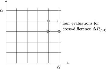
‘Levels’ in two-dimensional multi-index Monte Carlo application.

Multi-index Monte Carlo (MIMC) is probably the most significant extension of the MLMC methodology (Haji-Ali, Nobile and Tempone Reference Haji-Ali, Nobile and Tempone2014a ). In standard MLMC, there is a one-dimensional set of levels, with a scalar level index $\ell$ , although in some applications changing $\ell$ can change more than one aspect of the computation (such as both time-step and spatial discretization in a parabolic SPDE application, or time-step and number of sub-samples in a nested simulation). MIMC generalizes this to ‘levels’ being defined in multiple directions, so that the level ‘index’ $\boldsymbol{\ell }$ is now a vector of integer indices. This is illustrated in Figure 2.1 for a two-dimensional MIMC application.

In MLMC, if we define the backward difference

with $P_{-1}\equiv 0$ , as usual, then the telescoping sum which lies at the heart of MLMC is

Generalizing this to $D$ dimensions, Haji-Ali et al. (Reference Haji-Ali, Nobile and Tempone2014a ) first define a backward difference operator in one particular dimension,

where $\boldsymbol{e}_{d}$ is the unit vector in direction $d$ . They then define the cross-difference

and the telescoping sum becomes

As an example, Figure 2.1 marks the four locations at which $P_{\boldsymbol{\ell }}$ must be computed to determine the value of ${\bf\Delta}P_{(5,4)}$ in the two-dimensional application.

The MIMC theorem formulated by Haji-Ali et al. (Reference Haji-Ali, Nobile and Tempone2014a ) can be expressed in the following form to match, as closely as possible, the formulation of the MLMC theorem.

Figure 2.2.

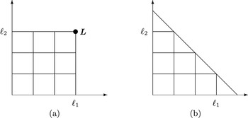
Two choices of two-dimensional MIMC summation region  ${\mathcal{L}}$ .

Notes.

• ∙ Condition (i) ensures weak convergence to the correct value.

• ∙ Condition (ii) ensures each $Y_{\boldsymbol{\ell }}$ has the correct expected value. This allows for the possibility of using an estimator which is more complicated than the natural choice $Y_{\boldsymbol{\ell }}={\bf\Delta}P_{\boldsymbol{\ell }}$ , if it will lead to a reduced variance.

• ∙ Conditions (iii) and (iv) give the order of convergence of the weak error and the multilevel correction variance, and condition (v) gives the rate at which the cost increases with level.

• ∙ The proof of the theorem is significantly harder than for the MLMC theorem.

• ∙ There is again the difficulty for each new application of determining ${\bf\alpha},{\bf\beta},{\bf\gamma}$ for conditions (iii)–(v). A relatively simple example will be given later in Section 9.

It might seem natural that the summation region ${\mathcal{L}}$ should be rectangular, as illustrated in Figure 2.2(a), so that

where $\boldsymbol{L}$ is the outermost point on the rectangle. However, Haji-Ali et al. (Reference Haji-Ali, Nobile and Tempone2014a ) prove that this gives the optimal order of complexity only when ${\it\eta}<0$ , and under the additional condition that

The optimal choice for ${\mathcal{L}}$ , which yields the complexity bounds given in the theorem, is of the form $\boldsymbol{\ell }\cdot \mathbf{n}\leq L$ for a particular choice of direction vector $\mathbf{n}$ with strictly positive components. In two dimensions, this corresponds to a triangular region, as illustrated in Figure 2.2(b). This is very similar to the use of sparse grid methods in high-dimensional PDE approximations (Bungartz and Griebel Reference Bungartz and Griebel2004), and indeed MIMC can be viewed as a combination of sparse grid methods and Monte Carlo sampling.

The benefits of MIMC over the standard MLMC can be very substantial. They are perhaps best illustrated by an elliptic PDE or SPDE example, in which $D$ corresponds to the number of spatial dimensions. Using the standard MLMC approach, ${\it\beta}$ , the rate of convergence of the multilevel variance, will usually be independent of  $D$ , but ${\it\gamma}$ , the rate of increase in the computational cost, will increase at least linearly with  $D$ . Therefore, in a high enough dimension we will have ${\it\beta}\leq {\it\gamma}$ and therefore the overall computational complexity will be less (often much less) than the optimal $O({\it\varepsilon}^{-2})$ . However, using MIMC we can have ${\it\beta}_{d}>{\it\gamma}_{d}$ in each direction, and therefore obtain the optimal complexity.

Hence, in the same way that sparse grids offer the possibility of dimension-independent complexity for deterministic PDE applications, MIMC offers the possibility of dimension-independent complexity for SPDEs and other high-dimensional stochastic applications.

2.5. Multi-dimensional output functionals

In Monte Carlo simulation, we start with a sample ${\it\omega}$ from the random input space, often compute an intermediate solution $U$ from an approximation to an SDE or SPDE, and then determine the final output quantity $P$ .

So far, the discussion in this article has focused on the idea of $P$ being a scalar output, but this is not necessarily always the case. In some applications there may be more than one scalar output of interest, and in other applications $P$ may be infinite-dimensional.

Table 2.1.

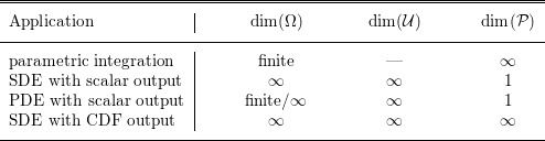
Dimensionality of ${\rm\Omega}$ , the input space, ${\mathcal{U}}$ , the intermediate solution space, and ${\mathcal{P}}$ , the output space, for some different MLMC applications.

Some of the possibilities are listed in Table 2.1. In Heinrich’s original multilevel research on parametric integration (Heinrich Reference Heinrich1998, Heinrich and Sindambiwe Reference Heinrich and Sindambiwe1999, Heinrich Reference Heinrich, Balakrishnan, Melas and Ermakov2000, Heinrich Reference Heinrich2001), the sample ${\it\omega}$ was from a finite-dimensional unit hypercube, there was no intermediate solution, and the output was an infinite-dimensional function of a parameter ${\it\lambda}$ . In the author’s initial research (Giles Reference Giles, Keller, Heinrich and Niederreiter2008a , Reference Giles2008b ), ${\it\omega}$ represented an infinite-dimensional input Brownian path, $U$ was the solution of an SDE, and $P$ was a scalar functional of that solution $U$ . In the simplest PDE applications, one might have a finite set of parameters which specify uncertain initial or boundary data, and a single scalar output, so only the intermediate PDE solution is infinite-dimensional. Finally, new research (Giles, Nagapetyan and Ritter Reference Giles, Nagapetyan and Ritter2015b ) addresses the problem of approximating the cumulative distribution function (CDF) of exit times associated with the solution of an SDE; in this case, all three spaces are infinite-dimensional.

The extension of the MLMC theory to a finite set of outputs is very natural. The standard MLMC theorem will apply to each one of the outputs. If there is a desired accuracy ${\it\varepsilon}_{m}$ for the $m$ th output, then a simple approach proposed by Tigran NagapetyanFootnote ¹ is to define

where $V_{\ell ,m}$ is the variance of the multilevel estimator on level $\ell$ for the $m$ th output. Enforcing the constraint

is then sufficient to ensure that all of the individual variance constraints are satisfied, and the standard Lagrange multiplier approach outlined in Section 1.3 can be used to determine the optimal number of samples to use on each level.

The extension of the theory to infinite-dimensional outputs requires the definition of an appropriate norm $\Vert \cdot \Vert$ , and then to a large extent the theory carries over by making the substitutions

One slight complication is that if $a$ and $b$ are two independent scalar random variables with zero mean, then

When using the 2-norm, this extends to independent random vectors $\boldsymbol{a}$ and $\boldsymbol{b}$ , each with zero mean, since

and similarly to random functions with a 2-norm based on an inner product. However this does not necessarily apply for other norms, and so the variance for the combined multilevel estimator cannot necessarily be expressed in the usual form as

Nevertheless, the theory can be extended to the use of other norms by using results from Banach space theory for the sums of independent random variables (Ledoux and Talagrand Reference Ledoux and Talagrand1991, Heinrich Reference Heinrich1998), and in recent research Daun and Heinrich have addressed the challenges of parametric integration in infinite-dimensional Banach spaces (Daun and Heinrich Reference Daun, Heinrich, Dick, Kuo, Peters and Sloan2013, Reference Daun and Heinrich2014a , Reference Daun and Heinrich2014b ).

2.6. Non-geometric MLMC

It is very important to repeat, and emphasize, the fact that MLMC does not require the use of a geometric sequence of grids. In many applications, and most of the existing literature, a geometric sequence will be the appropriate choice, but there are other applications for which it is not. The only assumptions in the analysis of the two-level method in Section 1.2 and the multilevel method in Section 1.3 are that the accuracy and cost increase with level, and the variance of the correction term decreases with level.

When there is no underlying structure to suggest that a geometric sequence is appropriate, a question which arises is how to select the levels. Suppose that one starts with a large collection of potential levels; how does one decide which subset to use?

One approach developed by Vidal-Codina, Nguyen, Giles and Peraire (Reference Vidal-Codina, Nguyen, Giles and Peraire2014) is to first use a number of trial samples to obtain an estimate of $V_{\ell }=\mathbb{V}[P_{\ell }]$ and $V_{\ell _{1},\ell _{2}}\equiv \mathbb{V}[P_{\ell _{2}}-P_{\ell _{1}}]$ for all pairs $(\ell _{1},\ell _{2})$ , with $\ell _{1}<\ell _{2}$ , with associated costs $C_{\ell }$ and $C_{\ell _{1},\ell _{2}}$ . For a particular ordered subset of levels, $\{\ell _{1},\ell _{2},\ldots ,\ell _{M}\}$ , with fixed $\ell _{M}=L$ to achieve a user-specified accuracy, following the analysis in Section 1.3 which led to (1.1), we obtain the cost

If the maximum number of levels is not too large, it is possible to perform an exhaustive search to find the optimal subset $\{\ell _{1},\ell _{2},\ldots ,\ell _{M}\}$ which minimizes this cost.

Alternatively, suppose that we have a multilevel Monte Carlo implementation with a number of levels $\ell =0,1,\ldots ,L$ . Looking in particular at one level $\ell$ , is it computationally more efficient to keep that level, or would it be better to drop it and jump straight from level $\ell -1$ to $\ell +1$ ?

If we keep level $\ell$ then the contribution to the overall multilevel estimator due to samples involving level $\ell$ is

The usual multilevel analysis shows that for optimality $N_{\ell }\propto \sqrt{V_{\ell }/C_{\ell }}$ , where $V_{\ell }\equiv \mathbb{V}[P_{\ell }-P_{\ell -1}]$ and $C_{\ell }$ is the cost of computing a single sample of $P_{\ell }-P_{\ell -1}$ . Hence we have

The combined variance from the two terms is

and the combined cost is

and so the product of the combined variance and combined cost is

On the other hand, if we drop level $\ell$ and jump straight from level $\ell -1$ to $\ell +1$ , then the replacement estimator is

Its variance is $\widetilde{V}_{\ell +1}/\widetilde{N}_{\ell +1}$ , where $\widetilde{V}_{\ell +1}\equiv \mathbb{V}[P_{\ell +1}-P_{\ell -1}]$ , and its cost is $\widetilde{N}_{\ell +1}\widetilde{C}_{\ell +1}$ , where $\widetilde{C}_{\ell +1}$ is the cost of a single sample of $P_{\ell +1}-P_{\ell -1}$ . Hence, the product of the variance and the cost is

The question now is whether

If this test is true, then it is best to drop level $\ell$ , because for a fixed computational cost this will deliver the lower variance, or for a fixed variance it can be achieved at a lower computational cost.

The main contribution to both $C_{\ell +1}$ and $\widetilde{C}_{\ell +1}$ comes from the level $\ell +1$ simulation which produces the output $P_{\ell +1}$ , so we will assume from here on that $\widetilde{C}_{\ell +1}\approx C_{\ell +1}$ . The cost ratio $C_{\ell }/C_{\ell +1}$ is usually known a priori, and the variance ratio $V_{\ell }/V_{\ell +1}$ is often known asymptotically as $\ell \rightarrow \infty$ , or can be estimated empirically. The key question is how $\widetilde{V}_{\ell +1}$ compares to $V_{\ell +1}$ . This could also be quantified empirically, by generating a few Monte Carlo samples for $P_{\ell +1}-P_{\ell -1}$ . Alternatively, we can perform some analysis to gain some insight into the question.

Using the standard result for the variance of a sum of two random variables, we have

where ${\it\rho}$ is the correlation between $P_{\ell +1}-P_{\ell }$ and $P_{\ell }-P_{\ell -1}$ . We can now consider two extremes, ${\it\rho}=1$ and ${\it\rho}=0$ .

If ${\it\rho}=1$ , and so we have perfect correlation between the increments at different levels, then

Since $C_{\ell }<C_{\ell +1}$ , it follows that the test (2.5) is never satisfied, and so it is best to retain level  $\ell$ . Near-perfect correlation is likely to arise in PDE applications with finite-dimensional uncertainty in the initial data, boundary data, or PDE coefficients. In this case, the increments $P_{\ell }-P_{\ell -1}$ obtained in going from one level to the next come from the progressive elimination of truncation error due to the discretization of the PDE.

On the other hand, if ${\it\rho}=0$ , and so the increments at different levels are independent, then $\widetilde{V}_{\ell +1}=V_{\ell +1}+V_{\ell }$ and so we drop level $\ell$ if

2.7. MLQMC

Giles and Waterhouse (Reference Giles and Waterhouse2009) developed a variant of MLMC which uses quasi-Monte Carlo samples instead of independent Monte Carlo samples. This was based on extensible rank-1 lattices developed at UNSW (Dick, Pillichshammer and Waterhouse Reference Dick, Pillichshammer and Waterhouse2007). QMC is known to be most effective for low-dimensional applications, and the numerical results were very encouraging for SDE applications in which the dominant computational cost was on the coarsest levels of resolution. However, there was no supporting theory for this research.

More recently, there has been considerable research on the theoretical foundations for multilevel QMC (MLQMC) methods; see Niu, Hickernell, Müller-Gronbach and Ritter (Reference Niu, Hickernell, Müller-Gronbach and Ritter2010), Kuo, Schwab and Sloan (Reference Kuo, Schwab and Sloan2015), Dick et al. (Reference Dick, Kuo and Sloan2013), Baldeaux and Gnewuch (Reference Baldeaux and Gnewuch2014) and Dick and Gnewuch (Reference Dick and Gnewuch2014a , Reference Dick and Gnewuch2014b ). These theoretical developments are very encouraging, showing that under certain conditions they lead to multilevel methods with a complexity which is $O({\it\varepsilon}^{-p})$ with $p<2$ .

3.1. MLMC algorithm

Based on the theory in Section 2.1, the geometric MLMC algorithm used for the numerical tests in this paper is given in Algorithm 1.

In the above algorithm, the equation for the optimal $N_{\ell }$ is

where $V_{\ell }$ is the estimated variance, and $C_{\ell }$ is the cost of an individual sample on level $\ell$ . This ensures that the estimated variance of the combined multilevel estimator is less than ${\it\varepsilon}^{2}/2$ .

The test for weak convergence tries to ensure that $|\mathbb{E}[P-P_{L}]|<{\it\varepsilon}/\sqrt{2}$ , to achieve an MSE which is less than ${\it\varepsilon}^{2}$ , with ${\it\varepsilon}$ being a user-specified RMS accuracy. If $\mathbb{E}[P_{\ell }-P_{\ell -1}]~\propto ~2^{-{\it\alpha}\ell }$ , then the remaining error is

This leads to the convergence test $|\mathbb{E}[P_{L}-P_{L-1}]|/(2^{{\it\alpha}}-1)<{\it\varepsilon}/\sqrt{2},$ but for robustness, we extend this check to extrapolate from the previous two data points $\mathbb{E}[P_{L-1}-P_{L-2}]$ , $\mathbb{E}[P_{L-2}-P_{L-3}]$ , and take the maximum over all three as the estimated remaining error.

It is important to note that this algorithm is heuristic; it is not guaranteed to achieve an MSE error which is less than ${\it\varepsilon}^{2}$ . The main MLMC theorem in Section 2.1 does provide a guarantee, but the conditions of the theorem assume a priori knowledge of the constants $c_{1}$ and $c_{2}$ governing the weak convergence and the variance convergence as $\ell \rightarrow \infty$ . These two constants are in effect being estimated in the numerical algorithm described above.

In addition, the accuracy of the variance estimate at each level depends on the size of the sample set. If it is small, then this variance estimate may be poor; we will see later that the implementation sets a minimum estimate by extrapolation from coarser levels with more samples.

3.2. Overview of MATLAB implementation

The results to be presented later all use the same two routines written in MATLAB.

• ∙ mlmc.m: driver code which performs the MLMC calculation using an application-specific routine to compute $\sum _{n}(P_{\ell }^{(n)}-P_{\ell -1}^{(n)})^{p}$ for $p=1,2$ and a specified number of independent samples.

• ∙ mlmc_test.m: a program which perform various tests and then calls mlmc.m to perform a number of MLMC calculations.

These two routines, and all of the application-specific routines, can be downloaded from Giles (Reference Giles2014).

3.3. MLMC test routine

mlmc_test.m first performs a set of calculations using a fixed number of samples on each level of resolution, and produces four plots:

• ∙ $\log _{2}(V_{\ell })$ versus level $\ell$ ,

• ∙ $\log _{2}(|\mathbb{E}[P_{\ell }-P_{\ell -1}]|)$ versus level $\ell$ ,

• ∙ consistency check versus level,

• ∙ kurtosis versus level.

The last two of these need some explanation. If $a,b,c$ are estimates for $\mathbb{E}[P_{\ell -1}^{f}]$ , $\mathbb{E}[P_{\ell }^{f}]$ , $\mathbb{E}[Y_{\ell }]$ , respectively, then it should be true that $a-b+c\approx 0$ . The consistency check verifies that this is true, to within the accuracy one would expect due to Monte Carlo sampling error. This is particularly important when $P_{\ell }^{f}\neq P_{\ell }^{c}$ because one is using different approximations on the coarse and fine levels.

Since

it computes and plots the ratio

where $V_{a},V_{b},V_{c}$ are empirical estimates for the variances of $a,b,c$ . The probability of this ratio being greater than unity is less than 0.3%. Hence, if it is, it indicates a likely programming error, or a mathematical error in the formulation which violates the crucial identity (2.4).

The MLMC approach needs a good estimate for $V_{\ell }=\mathbb{V}[Y_{\ell }]$ , but how many samples are needed for this? As few as 10 may be sufficient in many cases for a rough estimate, but many more are needed when there are rare outliers. When the number of samples $N$ is large, the standard deviation of the sample variance for a random variable $X$ with zero mean is approximately $\sqrt{({\it\kappa}-1)/N}~\mathbb{E}[X^{2}]$ , where the kurtosis ${\it\kappa}$ is defined as ${\it\kappa}=\mathbb{E}[X^{4}]/\mathbb{E}[X^{2}]\!)^{2}$ . Hence $O({\it\kappa})$ samples are required to obtain a reasonable estimate for the variance. As well as plotting the kurtosis ${\it\kappa}_{\ell }$ , mlmc_test.m will give a warning if ${\it\kappa}_{\ell }$ is very large, as this is an indication that the empirical variance estimate may be poor.

An extreme, but important, example is when $P$ always takes the value 0 or 1. In this case we have

If $p,q\ll 1$ , then $\mathbb{E}[X]\approx 0$ , and ${\it\kappa}\approx (p+q)^{-1}\gg 1$ . Therefore, many samples are required for a good estimate of $V_{\ell }$ ; otherwise, we may get all $X^{(n)}=0$ , which will give an estimated variance of zero. What is more, the kurtosis will become worse as $\ell \rightarrow \infty$ since $p,q\rightarrow 0$ due to weak convergence.

After performing these initial tests, mlmc_test.m then uses the driver routine mlmc.m to perform the MLMC computation for a number of values of ${\it\varepsilon}$ , and plots the results. These plots will be explained later when the first results are presented.

3.4. MLMC driver routine

The first part of the documentation section at the top of mlmc.m is fairly self-explanatory.

The user must supply an application-specific function to perform the calculations to compute $Y_{\ell }$ on level $\ell$ . This function has to conform to the following template.

The first part of the code initializes various parameters, and then uses the application-specific routine mlmc_l to generate the initial N0 samples on each of the first three levels.

The next part computes (or in later passes updates) the estimates for $m_{\ell }\equiv |\mathbb{E}[Y_{\ell }]|$ , and $V_{\ell }\equiv \mathbb{V}[Y_{\ell }]$ . If the mean and variance are decaying as expected, one would expect $m_{\ell }=2^{-{\it\alpha}}\,m_{\ell -1},~V_{\ell }=2^{-{\it\beta}}\,V_{\ell -1}$ . To avoid possible problems from high kurtosis generating poor empirical estimates, the estimates for $m_{\ell }$ and $V_{\ell }$ are not allowed to decrease by more than factor $1/2$ relative to this anticipated value.Footnote ²

If the user has not supplied the values for ${\it\alpha}$ and/or ${\it\beta}$ , they are now estimated by linear regression.

Next, the optimal number of samples on each level is computed, which in turn gives the number of additional samples which will need to be generated in the next pass.

In the final part of the loop, we test for weak convergence, using the algorithm described in Section 3.1. If a new level is added, its variance is estimated by extrapolation, and the optimal number of samples is updated.

The final step after the completion of the main loop is to compute the combined multilevel estimator.

3.5. MLQMC algorithm

We conclude this chapter with the description of an MLQMC algorithm which is based on that developed by Giles and Waterhouse (Reference Giles and Waterhouse2009), but updated to bring it more in line with the MLMC algorithm in Section 3.1.

The key change in MLQMC is that $N_{\ell }$ is now the size of a set of QMC points used on level $\ell$ . This set of points is not constructed randomly and independently but instead constructed very carefully, using well-established QMC techniques such as rank-1 lattices (Dick et al. Reference Dick, Pillichshammer and Waterhouse2007) or Sobol sequences (Joe and Kuo Reference Joe and Kuo2008) to provide a relatively uniform coverage of a unit hypercube integration region. In the best cases, this results in the approximate numerical integration error being $O(N_{\ell }^{-1})$ rather than the usual $O(N_{\ell }^{-1/2})$ error which comes from Monte Carlo sampling.

Using just one set of $N_{\ell }$ points gives good accuracy, but no confidence interval. To regain a confidence interval one uses randomized QMC in which the set of points is gives a random shift (for rank-1 lattice rules) or a digital scrambling (for Sobol sequences). Using 32 sets of points, each collectively randomized, yields 32 set averages for the quantity of interest, $Y_{\ell }$ , and from these 32 random independent values the variance of their average, $V_{\ell }$ , can be estimated in the usual way.

Since $V_{\ell }$ is now defined to be the variance of the average, for a given number of levels $L$ , the aim is to choose the $N_{\ell }$ in a way which ensures that

How can this be achieved most efficiently? Many QMC methods work naturally with $N_{\ell }$ as a power of 2. Doubling $N_{\ell }$ will usually eliminate a large fraction of the variance, so the greatest reduction in total variance relative to the additional computational effort is achieved by doubling $N_{\ell }$ on the level $\ell ^{\ast }$ given by

Based on this, and using the same test for weak convergence as in the MLMC algorithm, the MLQMC algorithm is given in Algorithm 2.

5.1. Euler–Maruyama discretization

The original multilevel path simulation paper (Giles Reference Giles2008b ) treated stochastic differential equations

using the simple Euler–Maruyama discretization with a uniform time-step $h$ and Brownian increments ${\rm\Delta}W_{n}$ ,

The multilevel Monte Carlo implementation is very simple. On level $\ell$ , the uniform time-step is taken to be $h_{\ell }=h_{0}\,M^{\ell }$ , for some integer  $M$ . The time-step $h_{0}$ on the coarsest level is often taken to be the interval length  $T$ , so that there is just one time-step for the entire interval, but this is not required, and in some applications using such a large time-step may lead to numerical results which are so inaccurate that they are not helpful, that is, they are such a poor control variate for the finer approximations that they do not lead to a reduction in the variance. In such cases, it would be better to start with a smaller value for  $h_{0}$ .

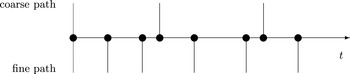
The multilevel coupling is achieved by using the same underlying driving Brownian path for the coarse and fine paths; this is accomplished by summing the Brownian increments for the fine path time-steps to obtain the Brownian increments for the coarse time-steps. The multilevel estimator is then the natural one defined in (2.2), with the specific payoff approximation $P_{\ell }$ depending on the particular application.

Provided the SDE satisfies the usual conditions (see Theorem 10.2.2 in Kloeden and Platen Reference Kloeden and Platen1992), the strong error for the Euler discretization with time-step $h$ is $O(h^{1/2})$ , so that

For Lipschitz payoff functions $P$ (such as European, Asian and lookback options in finance) for which

we have

and

and hence $V_{\ell }=O(h_{\ell })$ .

If $h_{\ell }=4^{-\ell }h_{0}$ , as in the numerical examples in Giles (Reference Giles2008b ), then this gives ${\it\alpha}=2$ , ${\it\beta}=4$ and ${\it\gamma}=2$ . Alternatively, if $h_{\ell }=2^{-\ell }h_{0}$ with twice as many time-steps on each successive level, as used in the numerical examples in this article, then ${\it\alpha}=1$ , ${\it\beta}=2$ and ${\it\gamma}=1$ . In either case, Theorem 2.1 gives the complexity to achieve an RMS error of ${\it\varepsilon}$ to be $O({\it\varepsilon}^{-2}(\log {\it\varepsilon})^{2})$ , which is near-optimal, because Creutzig, Dereich, Müller-Gronbach and Ritter (Reference Creutzig, Dereich, Müller-Gronbach and Ritter2009) prove an $O({\it\varepsilon}^{-2})$ lower bound for the complexity. The same paper also proves that MLMC achieves an $O({\it\varepsilon}^{-2}(\log {\it\varepsilon})^{2})$ worst-case optimal complexity for a class of Lipschitz path-dependent functions.

Figure 5.1.

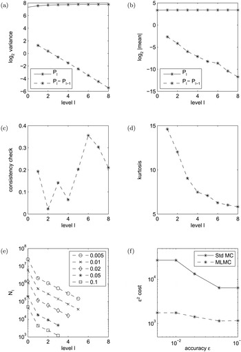
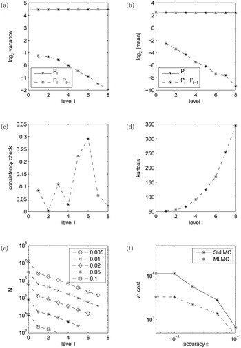
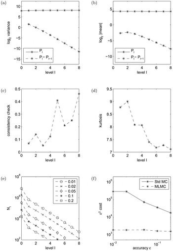
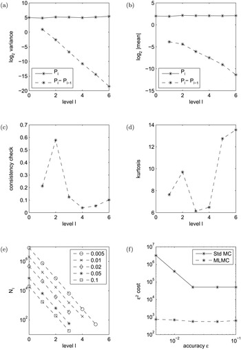
Numerical results for a European call option using the Euler–Maruyama discretization of the GBM SDE.

Figure 5.1 shows results for a financial call option with a single underlying asset satisfying the geometric Brownian motion SDE,

and payoff $P(S)\equiv \exp (-rT)\,\max (S_{T}-K,0)$ with $r=0.05,{\it\sigma}=0.2,T=1,S_{0}=100,K=100$ . The full code is provided in Giles (Reference Giles2014).

Plots (a) and (b) show the variance and absolute mean value for both $P_{\ell }$ and $P_{\ell }-P_{\ell -1}$ . These are based on an initial sample of $10^{5}$ paths. The line for $\log _{2}\mathbb{V}[P_{\ell }-P_{\ell -1}]$ in plot (a) has a slope of approximately $-1$ , corresponding to a variance proportional to $h_{\ell }$ , as expected. The line for $\log _{2}|\mathbb{E}[P_{\ell }-P_{\ell -1}]|$ also has a slope of approximately $-1$ , implying an $O(h_{\ell })$ weak convergence.

Plots (c) and (d) show the consistency check and kurtosis, as discussed in Section 3.3. These indicate that there is no problem with the consistency, and the kurtosis is actually improving slightly with level.

Plots (e) and (f) have the results from five separate MLMC calculations, each with a different specified accuracy ${\it\varepsilon}$ to be achieved. Plot (e) shows the number of samples which is used for each level of the MLMC computation. The number of levels increases as ${\it\varepsilon}$ decreases, as described in Section 3.1, to achieve the required weak error. The number of samples also varies with level, with many more on the coarsest level with just one time-step. On the finer levels, the optimal allocation of computational effort leads to $N_{\ell }\propto \sqrt{V_{\ell }/C_{\ell }}\approx 2^{-\ell }$ .

Plot (f) displays the total computational cost $C$ , multiplied by ${\it\varepsilon}^{2}$ . If $C$ were approximately proportional to ${\it\varepsilon}^{-2}$ then ${\it\varepsilon}^{2}\,C$ would be approximately constant. Indeed, this is what is seen, with the slight increase as ${\it\varepsilon}$ decreases being due to the $|\!\log {\it\varepsilon}|^{2}$ term in Theorem 2.1. For comparison, plot (f) also displays the cost using the standard Monte Carlo algorithm on the finest level used by the MLMC algorithm. The cost ratio is between 5 and 12, illustrating the benefits provided by the MLMC algorithm.

Figure 5.2.

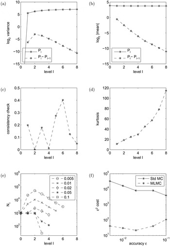
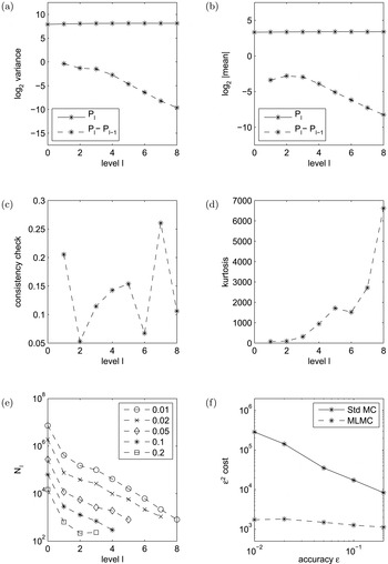
Numerical results for a digital call option using the Euler–Maruyama discretization of the GBM SDE.

Figure 5.2 illustrates the problem with discontinuous payoff functions. The underlying SDE is exactly the same, but the payoff is a digital option with payoff $P(S)\equiv 10\,\exp (-rT)\,H(S_{T}-K)$ , where $H(x)$ is the Heaviside step function. On the finer levels, most samples have fine and coarse paths which end on the same side of the strike $K$ , and hence give $P_{\ell }-P_{\ell -1}=0$ . However, noting that the strong error is $O(h_{\ell }^{1/2})$ , and there is a bounded density of paths terminating in the neighbourhood of $K$ , there is therefore an $O(h_{\ell }^{1/2})$ fraction of the samples with the coarse and fine paths on either side of the strike, with $P_{\ell }-P_{\ell -1}=\pm 1$ . This gives $V_{\ell }=O(h^{1/2})$ , and this lower rate of convergence is clearly visible in plot (a). Furthermore, $\mathbb{E}[(P_{\ell }-P_{\ell -1})^{4}]=O(h_{\ell }^{1/2})$ and so the kurtosis is $O(h_{\ell }^{-1/2})$ ; this increase in kurtosis is obvious in plot (d), which illustrates why this is a helpful quantity to plot. Consequently, this application has ${\it\alpha}=1$ , ${\it\beta}=1/2$ , ${\it\gamma}=1$ , leading to the MLMC complexity being $O({\it\varepsilon}^{-2.5})$ . This slightly worse complexity is visible in plot (f), and the computational savings compared to the standard Monte Carlo method are lower.

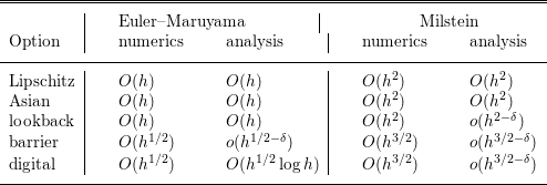
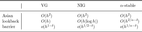
Table 5.1 summarizes the observed variance convergence rate in numerical experiments for a number of different financial options; the Asian option is based on the average value of the underlying asset, the lookback is based on its maximum or minimum value, and the barrier is a discontinuous function of the maximum or minimum. The table also displays the theoretical results which have been obtained; the digital option analysis is due to Avikainen (Reference Avikainen2009) while the others are due to Giles, Higham and Mao (Reference Giles, Higham and Mao2009).

Table 5.1.

Observed and theoretical convergence rates for the multilevel correction variance for scalar SDEs, using the Euler–Maruyama and Milstein discretizations. ${\it\delta}$ is any strictly positive constant.

Figure 5.3.

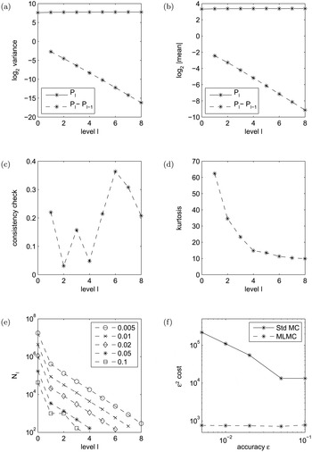
Numerical results for a European call option using the Milstein discretization of the GBM SDE.

5.2. Milstein discretization

For Lipschitz payoffs, the variance $V_{\ell }$ for the natural multilevel estimator converges at twice the order of the strong convergence of the numerical approximation of the SDE. This immediately suggests that it would be better to replace the Euler–Maruyama discretization by the Milstein discretization (Giles Reference Giles, Keller, Heinrich and Niederreiter2008a ) since it gives first-order strong convergence under certain conditions (see Theorem 10.3.5 in Kloeden and Platen Reference Kloeden and Platen1992).

For a scalar SDE the Milstein discretization is

and Figure 5.3 demonstrates the improved results obtained for the call option based on a single underlying GBM asset. $V_{\ell }$ is now $O(h_{\ell }^{2})$ , leading to ${\it\alpha}=1$ , ${\it\beta}=2$ , ${\it\gamma}=1$ , and there is a significant reduction in the total computational cost compared to MLMC using the Euler–Maruyama discretization.

Because ${\it\beta}>{\it\gamma}$ , the dominant computational cost is on the coarsest levels. Since these are low-dimensional, they are well suited to the use of quasi-Monte Carlo methods which are particularly effective in lower dimensions. This has been investigated by Giles and Waterhouse (Reference Giles and Waterhouse2009) using a rank-1 lattice rule to generate the quasi-random numbers, randomization with 32 independent offsets to obtain confidence intervals, and a standard Brownian bridge construction of the increments of the driving Brownian process. The numerical results showed that MLMC on its own was better than QMC on its own, but the combination of the two was even better. The QMC treatment greatly reduced the variance per sample for the coarsest levels, resulting in significantly reduced costs overall. In the simplest case of a Lipschitz European payoff, the computational complexity was reduced from $O({\it\varepsilon}^{-2})$ to approximately $O({\it\varepsilon}^{-1.5})$ .

5.3. Multi-dimensional SDEs

The discussion so far has been for scalar SDEs, but the computational benefits of Monte Carlo methods arise in higher dimensions. For multi-dimensional SDEs satisfying the usual commutativity condition (see, for example, p. 353 in Glasserman Reference Glasserman2004) the Milstein discretization requires only Brownian increments for its implementation, and most of the analysis above carries over very naturally.

The only difficulties are with lookback and barrier options, where the classical results for the distribution of the minimum or maximum of a one-dimensional Brownian motion do not extend to the joint distribution of the minima or maxima of two correlated Brownian motions. However, if the financial option depends on the weighted average of a set of underlying assets, then the Brownian interpolation for each individual asset leads naturally to a Brownian interpolation for the average, and then the standard one-dimensional results can be used as usual.

Figures 5.5 and 5.6 show results for lookback and barrier options based on five underlying assets. Full details of the numerical construction are given in Giles (Reference Giles, Rossetti, Hill, Johansson, Dunkin and Ingalls2009) and can also be viewed within the code Giles (Reference Giles2014). The MLMC variance is $O(h^{2})$ for the lookback option, and $O(h^{3/2})$ for the barrier option.

With multi-dimensional SDEs which do not satisfy the commutativity condition, the Milstein discretization requires the simulation of Lévy areas, iterated Itô integrals which can only be relatively easily simulated in two dimensions. This is an unavoidable problem; the classical result of Clark and Cameron (Reference Clark, Cameron and Grigelionis1980) proves that $O(h^{1/2})$ strong convergence is the best that can be achieved in general using only Brownian increments.

Nevertheless, Giles and Szpruch (Reference Giles and Szpruch2014) have developed an antithetic treatment which achieves a very low variance despite the $O(h^{1/2})$ strong convergence. The estimator which is used is

Here ${\it\omega}_{i}$ represents the driving Brownian path, and ${\it\omega}_{i}^{a}$ is an antithetic counterpart defined by a time-reversal of the Brownian path within each coarse time-step. This results in the Brownian increments for the antithetic fine path being swapped relative to the original path. Lengthy analysis proves that the average of the fine and antithetic paths is within $O(h)$ of the coarse path, and hence the multilevel variance is $O(h^{2})$ for smooth payoffs, and $O(h^{3/2})$ for the standard European call option.

This treatment has been extended to handle lookback and barrier options (Giles and Szpruch Reference Giles, Szpruch, Dick, Kuo, Peters and Sloan2013). This combines sub-sampling of the Brownian path to approximate the Lévy areas with sufficient accuracy to achieve $O(h^{3/4})$ strong convergence, with an antithetic treatment at the finest level of resolution to ensure that the average of the fine paths is within $O(h)$ of the coarse path.

5.4. Computing sensitivities

In computational finance, it is important to be able to compute sensitivities in addition to option prices. When the option payoff is continuous, the standard Monte Carlo approach is pathwise sensitivity analysis (Broadie and Glasserman Reference Broadie and Glasserman1996) (developed earlier as Infinitesimal Perturbation Analysis: see L’Ecuyer Reference L’Ecuyer1990), which considers linearized perturbations to the underlying path evolution, and the consequential perturbation to the payoff.

From a multilevel Monte Carlo point of view, the difficulty that this introduces is that the derivative of a call option payoff function is discontinuous. Hence, computing first-order sensitivities for a call option has similar difficulties to computing the option price for a digital option. Sensitivities for digital options can be obtained by first using the conditional expectation approach described previously, and then applying pathwise sensitivity analysis to this.

Full details on how to formulate appropriate MLMC estimators are given by Burgos and Giles (Reference Burgos, Giles, Plaskota and Woźniakowski2012), and the numerical analysis of the resulting variance is given by Burgos (Reference Burgos2014).

5.5. Exit times and Feynman–Kac formula

The simplest one-dimensional form of the Feynman–Kac formula states that if $u(x,t)$ is the solution of the parabolic PDE

for $x\in V$ , subject to the terminal condition $u(x,T)=f(x)$ , and the boundary condition $u(x,t)=g(x)$ for $x\in \partial V$ , then $u(x,t)$ can also be written as the conditional expectation

where $S_{t}$ satisfies the SDE

and ${\it\tau}$ is the exit time

Because of this formula and its multi-dimensional generalization, and also because of other applications which are concerned with the time at which particles exit a particular domain, there is considerable interest in the estimation of exit times.

Higham et al. (Reference Higham, Mao, Roj, Song and Yin2013) consider the estimation of $\mathbb{E}[{\it\tau}]$ using a multilevel approximation based on an Euler–Maruyama discretization. They prove that this can be achieved for very general multi-dimensional SDEs at a computational cost which is $O({\it\varepsilon}^{-3}|\!\log {\it\varepsilon}|^{1/2})$ . This is better than the $O({\it\varepsilon}^{-4})$ complexity of a standard Monte Carlo simulation using the same numerical approximation of the exit time, but is not better than the complexity achieved by Gobet and Menozzi (Reference Gobet and Menozzi2010) using a Monte Carlo simulation with a boundary correction which improves the weak order of convergence to first order.

Earlier research by Primozic (Reference Primozic2011) demonstrates an $O({\it\varepsilon}^{-2})$ complexity for a one-dimensional problem. This builds on the Milstein approximation for barrier options developed by Giles (Reference Giles, Keller, Heinrich and Niederreiter2008a ), using the approximate Brownian interpolation to determine the approximate probability that the underlying path crosses the boundary within each time-step. This improves both the weak convergence and the multilevel variance, giving ${\it\alpha}=1$ , ${\it\beta}=3/2$ and ${\it\gamma}=1$ . This approach is capable of being extended to multi-dimensional SDEs which satisfy the commutativity condition which allows the use of the Milstein discretization without requiring the simulation of Lévy areas.

5.6. Stiff and highly nonlinear SDEs

In the numerical examples presented above, it is possible to use only one time-step on the coarsest level of approximation, and still obtain a sufficiently accurate path simulation so that the resulting payoff approximation is a useful control variate for the next level of approximation.

However, in other applications this may not be true. If the drift term has a characteristic time-scale of ${\it\tau}$ , as in a mean-reverting drift $({\it\theta}-S_{t})/{\it\tau}$ , then when using the explicit Euler–Maruyama discretization the time-step $h_{0}$ on the coarsest level cannot be much larger than ${\it\tau}$ without encountering severe numerical stability problems. This is a natural restriction shared by explicit discretizations of ordinary differential equations.

A related problem is addressed by Hutzenthaler, Jentzen and Kloeden (Reference Hutzenthaler, Jentzen and Kloeden2013), who are concerned with SDEs such as

which have a super-linear growth in the drift and/or the volatility. This again leads to numerical instability if a uniform time-step is used. Their solution is to introduce a slight modification to the Euler–Maruyama discretization which limits the size of the drift term on each level of approximation when $S_{t}$ is large, to avoid this instability.

Other approaches to these problems include the use of drift-implicit methods (Dereich, Neuenkirch and Szpruch Reference Dereich, Neuenkirch and Szpruch2012, Higham, Mao and Stuart Reference Higham, Mao and Stuart2002), or a change or variables equivalent to the use of an integrating factor in ODEs (see the Heston treatment in Giles (Reference Giles, Keller, Heinrich and Niederreiter2008a ) which was suggested by Mark Broadie).

Another important approach, when the difficulties are only for extreme value of $S_{t}$ , or for a short time interval, is to use adaptive time-stepping. Hoel, von Schwerin, Szepessy and Tempone (Reference Hoel, von Schwerin, Szepessy, Tempone, Engquist, Runborg and Tsai2012, Reference Hoel, von Schwerin, Szepessy and Tempone2014) construct a multilevel adaptive time-stepping discretization in which, for each stochastic instance ${\it\omega}$ , the time-steps used on level $\ell$ are a subdivision of those used on level $\ell -1$ , which in turn are a subdivision of those on level $\ell -2$ , and so on. By doing this, the payoff $P_{\ell }$ on level $\ell$ is the same regardless of whether one is computing $P_{\ell }-P_{\ell -1}$ or $P_{\ell +1}-P_{\ell }$ , and therefore the MLMC telescoping summation is respected. Another notable aspect of their work is the use of adjoint/dual sensitivities to determine the optimal time-step size.

New unpublished work by Giles, Süli, Whittle and Ye implements adaptive time-stepping slightly differently. Instead of the time-steps on one level being a subdivision of those on the level above, it uses a completely independent adaptation on each level of refinement, with an adaptive time-step of the form

where $H(S)$ is independent of level. This results in time-steps which are not naturally nested. It may appear that this would cause difficulties in the MLMC implementation, but Figure 5.7 tries to illustrate that it does not. The underlying Brownian path needs to be sampled at a set of times which are the union of the simulation times used by the coarse and fine path. The independent Brownian increments can be simulated for each time interval, and summed to give $W(t)$ at the required times. An outline algorithm to implement this is given in Algorithm 3.

Figure 5.7.

Generation of Brownian increments for a multilevel simulation with adaptive time-stepping.

5.7. CDF and density estimation

In some applications the objective is an estimation of the cumulative distribution function (CDF) or density of an output quantity  $P$ , rather than its expected value.

Kebaier and Kohatsu-Higa (Reference Kebaier and Kohatsu-Higa2008) addressed the problem of constructing pointwise estimates of the density of the SDE solution $S_{T}$ , using Malliavin calculus and a two-level variance reduction based on Kebaier’s earlier work (Kebaier Reference Kebaier2005).

Motivated by an interesting engineering application (Iliev, Nagapetyan and Ritter Reference Iliev, Nagapetyan and Ritter2013), a multilevel approach to CDF and density estimation for arbitrary output functions has been developed by Giles et al. (Reference Giles, Nagapetyan and Ritter2015b ). The CDF of a scalar output $P$ is represented approximately by a polynomial spline function. Pointwise values of the CDF which are used as knot values in the spline construction correspond to expected values of an indicator function,

where $H(x)$ is the Heaviside step function. To improve the multilevel variance, this is smoothed to give

where $g(x)$ is a continuous function with $g(x)=0$ for $x<-1$ , and $g(x)=1$ for $x>1$ . The parameter ${\it\delta}$ controls the degree of smoothing. As ${\it\delta}\rightarrow 0$ , $g(x/{\it\delta})\rightarrow H(x)$ , and the accuracy improves but the variance of the multilevel estimator increases. Hence, this application has both spline approximation and smoothing errors in addition to the usual discretization and sampling errors. Balancing these errors gives the best accuracy for a given computational cost. The MLMC approach gives a substantial improvement in the order of complexity, and numerical examples demonstrate the savings which can be achieved.

The same paper also discusses the extension to density estimation. In this case, the density ${\it\rho}(x)$ of the scalar output $P$ is given by

where $g(x)$ is a continuous function with $g(x)=0$ for $|x|>1$ , and

This has similarities with kernel density estimation (Silverman Reference Silverman1986), and can also be generalized to multi-dimensional outputs.

6.1. Jump-diffusion processes

With finite activity jump-diffusion processes, such as in the Merton model (Merton Reference Merton1976), it is natural to simulate each individual jump using a jump-adapted discretization (Mikulevicius and Platen Reference Mikulevicius and Platen1988, Platen and Bruti-Liberati Reference Platen and Bruti-Liberati2010) in which the Brownian diffusion between each jump is approximated using an Euler–Maruyama or Milstein approximation, and then each jump is simulated exactly.

If the jump activity rate is constant, then for each stochastic sample ${\it\omega}$ the jumps on the coarse and fine paths will occur at the same time, and therefore the extension of the multilevel method is straightforward with the coarse and fine paths using the same underlying Brownian paths, and the same random variables to determine the jump times and strengths (Xia and Giles Reference Xia, Giles, Plaskota and Woźniakowski2012).

If the jump rate is path-dependent then the situation is trickier. If there is a known upper bound to the jump rate, then one can use the ‘thinning’ approach of Glasserman and Merener (Reference Glasserman and Merener2004) in which a set of candidate jump times is simulated based on the constant upper bound, and then a subset of these are selected to be real jumps. The problem with the multilevel extension of this is that some candidate jumps will be selected for the coarse path but not for the fine path, or vice versa, leading to an $O(1)$ difference in the paths and hence the payoffs. Xia and Giles (Reference Xia, Giles, Plaskota and Woźniakowski2012) avoid this by using a change of measure to ensure that the jump times are the same for both paths; this introduces a Radon–Nikodym derivative into the payoff evaluation, but significantly reduces the multilevel correction variance.

6.2. More general processes

With infinite activity Lévy processes it is impossible to simulate each jump. One approach is to simulate the large jumps and either neglect the small jumps or approximate their effect by adding a Brownian diffusion term (Dereich Reference Dereich2011, Dereich and Heidenreich Reference Dereich and Heidenreich2011, Marxen Reference Marxen2010). Following this approach, the cutoff ${\it\delta}_{\ell }$ for the jumps which are simulated varies with level, and ${\it\delta}_{\ell }\rightarrow 0$ as $\ell \rightarrow \infty$ to ensure that the bias converges to zero. In the multilevel treatment, when simulating $P_{\ell }-P_{\ell -1}$ the jumps fall into three categories. The ones which are larger than ${\it\delta}_{\ell -1}$ get simulated in both the fine and coarse paths. The ones which are smaller than ${\it\delta}_{\ell }$ are either neglected for both paths or approximated by the same Brownian increment. The difficulty is in the intermediate range $[{\it\delta}_{\ell },{\it\delta}_{\ell -1}]$ , in which the jumps are simulated for the fine path but neglected or approximated for the coarse path. This is what leads to the difference in path simulations, and contributes to a non-zero value for $P_{\ell }-P_{\ell -1}$ .

Table 6.1.

Numerical analysis convergence rates for the multilevel variance $V_{\ell }\equiv \mathbb{V}[P_{\ell }-P_{\ell -1}]$ for variance-gamma, NIG, and spectrally negative ${\it\alpha}$ -stable processes and different financial options. ${\it\delta}$ is any strictly positive constant.

Alternatively, for many SDEs driven by a Lévy process it is possible to directly simulate the increments of the Lévy process over a set of uniform time-steps (Schoutens Reference Schoutens2003), in exactly the same way as one simulates Brownian increments. When estimating the price of European options which depend only on the final value of the Lévy process, there is no need for MLMC as one can directly simulate the final value. However, multilevel is still very useful for path-dependent financial options such as Asian, lookback and barrier options, and there has been good progress in the numerical analysis of these applications (Xia Reference Xia2014, Xia and Giles Reference Xia and Giles2014). Table 6.1 gives the convergence rates obtained from the numerical analysis; numerical experiments support these results but suggest they may not be sharp in some cases.

For other Lévy processes, it may be possible in the future to simulate the increments by constructing near-perfect (i.e., to within the limits of finite precision computer arithmetic) approximations to the inverse of the cumulative distribution function. Where this is possible, it may be the best approach to achieve a perfect coupling between the coarse and fine path simulations, since the increments of the driving Lévy process for the coarse path can be obtained trivially by summing the increments for the fine path.

Finally, we mention the work of Ferreiro-Castilla, Kyprianou, Scheichl and Suryanarayana (Reference Ferreiro-Castilla, Kyprianou, Scheichl and Suryanarayana2014), who develop a multilevel approach for barrier options using a Wiener–Hopf factorization technique to sample exactly from the joint distribution of the terminal value of a Lévy process at an exponential random stopping time, and its maximum (or minimum) over the intervening interval. The particularly novel aspect here is the random terminal time; by using multiple shorter random periods it is possible, because of the Central Limit Theorem, to get closer to a desired fixed terminal time, but at an increased cost. In the multilevel coupling, the thinning approach of Glasserman and Merener (Reference Glasserman and Merener2004) is again used to link the coarse and fine path simulations. Numerical analysis for lookback options gives a complexity which is $O({\it\varepsilon}^{-3})$ for processes of bounded variation, and $O({\it\varepsilon}^{-4})$ for processes of unbounded variation. Numerical experiments for barrier options demonstrate a similar complexity.

7.1. Two simple examples

The MATLAB codes accompanying this article include two simple PDE examples.

The first is really a boundary-value ODE application, but it can be viewed as a one-dimensional elliptic PDE, with random coefficients and random forcing. The equation is

on $0<x<1$ , with boundary data $u(0)=u(1)=0$ . $Z$ is a normal random variable with zero mean and unit variance, and

with $a$ being a uniform random variable on the unit interval $(0,1)$ . The output quantity of interest is chosen to be

The multilevel implementation is very easy. Level $\ell$ uses a uniform grid with spacing $h_{\ell }=2^{-(\ell +1)}$ , so there is just one interior grid point on the coarsest level. A simple second-order central difference approximation is used (equivalent to a finite element approximation with a 1-point quadrature).

The uniform second-order accuracy means that there is a constant $K$ such that $|P-P_{\ell }|<K\,h_{\ell }^{2},$ and therefore we have ${\it\alpha}=2$ , ${\it\beta}=4$ and ${\it\gamma}=1$ , resulting in an $O({\it\varepsilon}^{-2})$ complexity. All of these features can be verified in the numerical results in Figure 7.1.

The second example is a one-dimensional parabolic SPDE, in which $u(x,t)$ satisfies the SPDE

on the domain $0<x<1$ with boundary data $u(0,t)=u(1,t)=0$ and initial data $u(x,0)=0$ . The output functional is chosen to be

The multilevel implementation is again very easy. An Euler–Maruyama time discretization with time-step $k$ , combined with a second-order space discretization with uniform grid spacing $h$ , gives the discrete approximation

The level $\ell$ approximation uses

Keeping $k_{\ell }/h_{\ell }^{2}=1/4$ ensures the explicit numerical discretization is stable on all levels. Since the number of grid points doubles on each level, and the number of time-steps increases by factor 4, the cost per sample increases by factor 8, giving ${\it\gamma}=3$ .

Because the stochastic forcing is additive, that is, the volatility does not depend on $u(x,t)$ , the Euler–Maruyama discretization is actually equivalent to a Milstein discretization and hence the time discretization errors are $O(k)$ . This is of the same order as the spatial discretization errors which are $O(h^{2})$ , and therefore the solution error is $O(2^{-2\ell })$ and hence ${\it\alpha}=2$ and ${\it\beta}=4$ . This leads to the optimal complexity of $O({\it\varepsilon}^{-2})$ .

These features are again confirmed in the numerical results shown in Figure 7.2.

Figure 7.2.

Numerical results for a one-dimensional parabolic SPDE with Brownian forcing.

7.2. Elliptic SPDE

The largest amount of research on multilevel for SPDEs has been for elliptic PDEs with random coefficients. The PDE typically has the form

with Dirichlet or Neumann boundary conditions on the boundary $\partial D$ . For subsurface flow problems, such as the modelling of groundwater flow in nuclear waste repositories, the diffusivity (or permeability) ${\it\kappa}$ is often modelled as a log-normal random field, that is, $\log {\it\kappa}$ is a Gaussian field with a uniform mean (which we will take to be zero for simplicity) and a covariance function of the general form $R(\mathbf{x},\mathbf{y})=r(\mathbf{x}-\mathbf{y})$ . Samples of $\log k$ are provided by a Karhunen–Loève expansion,

where ${\it\theta}_{n}$ are the eigenvalues of $R(\mathbf{x},\mathbf{y})$ in decreasing order, $f_{n}$ are the corresponding eigenfunctions, and ${\it\xi}_{n}$ are independent unit normal random variables. However, it is more efficient to generate them using a circulant embedding technique which enables the use of FFTs (Dietrich and Newsam Reference Dietrich and Newsam1997).

The multilevel treatment is straightforward. The spatial grid resolution is doubled on each level. Using the Karhunen–Loève generation, the expansion is truncated after $K_{\ell }$ terms, with $K_{\ell }$ increasing with level (Teckentrup et al. Reference Teckentrup, Scheichl, Giles and Ullmann2013); a similar approach has also been used with the circulant embedding generation.

In both cases, $\log {\it\kappa}$ is generated using a row-vector of independent unit normal random variables ${\it\xi}$ . The variables for the fine level can be partitioned into those for the coarse level ${\it\xi}_{\ell -1}$ , plus some additional variables $z_{\ell }$ , giving ${\it\xi}_{\ell }=({\it\xi}_{\ell -1},z_{\ell })$ .

The numerical analysis of the multilevel approach for these elliptic SPDE applications is challenging because the diffusivity is unbounded, but Charrier et al. (Reference Charrier, Scheichl and Teckentrup2013) have successfully analysed it for certain output functionals, and Teckentrup et al. have further developed the analysis for other output functionals and more general log-normal diffusivity fields (Teckentrup et al. Reference Teckentrup, Scheichl, Giles and Ullmann2013, Teckentrup Reference Teckentrup2013).

7.3. Parabolic SPDE

Giles and Reisinger (Reference Giles and Reisinger2012) consider an unusual SPDE from credit default modelling,

subject to boundary condition $p(0,t)=0$ . Here $p(x,t)$ represents the probability density function for firms being a distance $x$ from default at time $t$ . The diffusive term is due to idiosyncratic factors affecting individual firms, while the stochastic term due to the scalar Brownian motion $M_{t}$ corresponds to the systemic movement due to random market effects on all firms. The payoff corresponds to different tranches of a credit derivative which depends on the integral $\int _{0}^{\infty }p(x,t)~\text{d}x$ at a set of discrete times.

A Milstein time discretization with time-step $k$ , and a central space discretization of the spatial derivatives with uniform spacing $h$ give the numerical approximation

where $p_{j}^{n}\approx p(j\,h,n\,k)$ , and the $Z_{n}$ are standard normal random variables so that $\sqrt{h}~Z_{n}$ corresponds to an increment of the driving scalar Brownian motion.

The multilevel implementation is very straightforward. As with the model parabolic example discussed previously, $k_{\ell }=k_{\ell -1}/4$ and $h_{\ell }=h_{\ell -1}/2$ due to numerical stability considerations which are analysed in the paper. The coupling between the coarse and fine samples comes from summing the fine path Brownian increments to give the increments for the coarse path, exactly the same as for SDEs The computational cost increases by factor 8 on each level, and numerical experiments indicate that the variance decreases by factor 8, so the overall computational complexity to achieve an $O({\it\varepsilon})$ RMS error is again $O({\it\varepsilon}^{-2}(\log {\it\varepsilon})^{2})$ .

This work has been extended by Bujok and Reisinger (Reference Bujok and Reisinger2012) to include a systemic jump-diffusion term. They also switch from continuous monitoring of default, which gives the boundary condition $p(0,t)=0$ for all $t$ , to discrete monitoring which introduces the boundary condition $p(x,t)=0$ for $x\leq 0$ for each discrete default date  $t$ .

7.4. Reduced basis approximation

New research by Vidal-Codina et al. (Reference Vidal-Codina, Nguyen, Giles and Peraire2014) uses a very different approach to SPDE approximation. They start with a high-accuracy finite element approximation

where ${\it\omega}$ represents the dependence on the stochastic input parameters. They then use a reduced basis approximation with a fixed set of basis functions  $\mathbf{u}_{k}$

which leads to a much smaller system of equations

The output of interest is a function of the solution, so that they are interested in estimating $\mathbb{E}[f(\mathbf{u})]$ . There is an accuracy–cost tradeoff here: larger values for $K$ lead to greater accuracy, but at a much larger cost. The MLMC treatment makes $K$ a function of the level $\ell$ , so that most simulations are performed with a small value for $K$ , and relatively few with a large value.

In this application, geometric MLMC is not appropriate and so they face the question of how to choose the levels. As discussed already in Section 2.6, they start with a set of candidate levels and use a number of trial samples to obtain an estimate of the variances $V_{\ell _{1},\ell _{2}}\equiv \mathbb{V}[P_{\ell _{1}}-P_{\ell _{2}}]$ for all pairs of levels. They then use this to determine the optimal subset of levels for the main computation.

9.1. MLMC treatment

In nested simulations we are interested in estimating quantities of the form

where $Z$ is an outer random variable, and $\mathbb{E}_{W}[g(Z,W)]$ is a conditional expectation with respect to an independent inner random variable  $W$ .

For example, in some financial applications $Z$ which represents different risk scenarios, $\mathbb{E}_{W}[g(Z,W)]$ represents exposure, conditional on the scenario $Z$ , and $f$ might correspond to the loss in excess of the capital reserves, so that $\mathbb{E}_{Z}[f(\mathbb{E}_{W}[g(Z,W)])]$ is the expected shortfall.

This can be simulated using nested Monte Carlo simulation with $N$ outer samples $Z^{(n)}$ , $M$ inner samples $W^{(m,n)}$ and a standard Monte Carlo estimator:

Note that to improve the accuracy of the estimate we need to increase both $M$ and $N$ , and this will significantly increase the cost.

An MLMC implementation is straightforward; on level $\ell$ we can use $M_{\ell }=2^{\ell }$ inner samples. To construct a low-variance estimate for $\mathbb{E}[P_{\ell }-P_{\ell -1}]$ where

we use an antithetic approach, and split the $M_{\ell }$ samples of $W$ for the ‘fine’ value into two subsets of size $M_{\ell -1}$ for the ‘coarse’ value:

Note that this has the correct expectation, that is, $\mathbb{E}[Y_{\ell }]=\mathbb{E}[P_{\ell }-P_{\ell -1}]$ .

If we define

then if $f$ is twice differentiable a Taylor series expansion gives

By the Central Limit Theorem, ${\rm\Delta}g_{1}^{(n)},{\rm\Delta}g_{2}^{(n)}=O(M_{\ell }^{-1/2})$ and therefore

It follows that $\mathbb{E}[Y_{\ell }]=O(M_{\ell }^{-1})$ and $V_{\ell }=O(M_{\ell }^{-2})$ . For the MLMC theorem, this corresponds to ${\it\alpha}=1$ , ${\it\beta}=2$ , ${\it\gamma}=1$ , so the complexity is $O({\it\varepsilon}^{-2})$ .

This antithetic approach to nested simulation has been developed independently by several authors (Haji-Ali Reference Haji-Ali2012, Chen and Liu Reference Chen and Liu2012, Bujok, Hambly and Reisinger Reference Bujok, Hambly and Reisinger2013).

Haji-Ali (Reference Haji-Ali2012) used it in a mean field model for the motion of crowds, in which each person is modelled as a independent agent subject to random forcing and an additional force due to the collective influence of the crowd. This same approach is also relevant to mean field problems which arise in plasma physics (Rosin et al. Reference Rosin, Ricketson, Dimits, Caflisch and Cohen2014).

Bujok et al. (Reference Bujok, Hambly and Reisinger2013) used multilevel nested simulation for a financial credit derivative application. In their case, the function $f$ was piecewise linear, not twice differentiable, and so the rate of variance convergence was slightly lower, with ${\it\beta}=1.5$ . However, this is still sufficiently large to achieve an overall complexity which is $O({\it\varepsilon}^{-2})$ .

The pricing of American options is one of the big challenges for Monte Carlo methods in computational finance, and Belomestny, Schoenmakers and Dickmann (Reference Belomestny, Schoenmakers and Dickmann2013) have developed a multilevel Monte Carlo for this purpose, based on Anderson and Broadie’s dual simulation method (Andersen and Broadie Reference Andersen and Broadie2004) in which a key component at each time-step in the simulation is to estimate a conditional expectation using a number of sub-paths. In their multilevel treatment, Belomestny et al. (Reference Belomestny, Schoenmakers and Dickmann2013) use the same uniform time-step on all levels of the simulation, so the quantity which changes between different levels of simulation is the number of sub-samples used to estimate the conditional expectation. Hence, their work is another example of nested simulation.

9.2. MIMC treatment

The analysis in the previous section assumes that we can compute $g(Z,W)$ with $O(1)$ cost, but suppose now that $W$ represents a complete Brownian path, and so $g(Z,W)$ cannot be evaluated exactly; it can only be approximated by using some finite number of time-steps. We could continue to use MLMC, and on level $\ell$ we could use $2^{\ell }$ time-steps. When using the Milstein discretization (giving first-order weak and strong convergence) this would still give ${\it\alpha}=1$ , ${\it\beta}=2$ . However, we would now have ${\it\gamma}=2$ , because the work on successive levels would go up by factor $4\times$ , because of using twice as many time-steps as well as twice as many inner samples. This then leads to an overall MLMC complexity which is $O({\it\varepsilon}^{-2}(\log {\it\varepsilon})^{-2})$ .

Instead we can use MIMC, to get back to an optimal complexity of $O({\it\varepsilon}^{-2})$ . We now have a pair of level indices $(l_{1},l_{2})$ , with the number of inner samples equal to $2^{\ell _{1}}$ and the number of time-steps proportional to $2^{\ell _{2}}$ . If we use the natural extension of the MLMC estimator to the corresponding MIMC estimator, which means (for $l_{1}>0,l_{2}>0$ ) using

The subscript on the $g$ terms denotes the level of time-step approximation.

Carrying out the same analysis as before, performing the Taylor series expansion around $\mathbb{E}[g(Z^{(n)},W)]$ , we obtain

The difference of squares can be rearranged as

Due to the Central Limit Theorem, we have

and assuming first-order strong convergence we also have

Combining these results, we obtain

and therefore $\mathbb{E}[Y_{\ell }]=O(2^{-\ell _{1}-\ell _{2}})$ and $V_{\ell }=O(2^{-2\ell _{1}-2\ell _{2}})$ with a cost per sample which is $O(2^{\ell _{1}+\ell _{2}})$ . In Theorem 2.2 this corresponds to ${\it\alpha}_{1}={\it\alpha}_{2}=1$ , ${\it\beta}_{1}={\it\beta}_{2}=2$ , and ${\it\gamma}_{1}={\it\gamma}_{2}=1$ , so the overall complexity is $O({\it\varepsilon}^{-2})$ .

Following the analysis in Bujok et al. (Reference Bujok, Hambly and Reisinger2013), if the function $f$ is continuous and piecewise differentiable, rather than being twice differentiable, then in the MLMC treatment we would get ${\it\beta}=1.5$ , and hence an overall complexity which is $O({\it\varepsilon}^{-2.5})$ . On the other hand, with MIMC we would have ${\it\beta}_{1}={\it\beta}_{2}=1.5$ and so the complexity would remain $O({\it\varepsilon}^{-2})$ . This illustrates the benefit of the MIMC approach compared to standard MLMC.

10.1. Markov chains and limiting distributions

In new research, Glynn and Rhee (Reference Glynn and Rhee2014) consider the application of their randomized version of MLMC to Markov chains, and in particular they have addressed the problem of estimating quantities which are expectations with respect to a limiting distribution. In their application, the Markov chain $\{X_{n}\}$ in a metric space with metric $d$ is defined by

where $\{{\it\phi}_{n}\}$ is a sequence of i.i.d. random functions. Furthermore, it is assumed that the ${\it\phi}$ are contracting on average in the sense that

for some ${\it\gamma}\in (0,1)$ . Under these conditions, it is known that the distribution of $X_{n}$ converges weakly to that of a limit random variable $X_{\infty }$ , and their objective is to estimate expectations of the form $\mathbb{E}[f(X_{\infty })]$ , where $f$ is Hölder-continuous with exponent ${\it\gamma}$ , so that $|f(y)-f(x)|\leq d(x,y)^{{\it\gamma}}.$

An example they offer of a chain satisfying the required conditions is

where $\mathbb{P}({\it\xi}_{n}=0)=\mathbb{P}({\it\xi}_{n}=1)=1/2$ . The invariant distribution in this case is the uniform distribution on $[0,2]$ .

Figure 10.1.

Level $\ell$ and $\ell -1$ paths for contracting Markov chains.

In the standard MC approach, one would approximate $\mathbb{E}[f(X_{\infty })]$ by estimating $\mathbb{E}[f(X_{N})]$ for some large value of $N$ , but this would be a biased estimate. Glynn and Rhee (Reference Glynn and Rhee2014) circumvent this problem by making $N$ increase with level, starting a level $\ell$ simulation at $n=-N_{\ell }$ and terminating it at $n=0$ , as illustrated in Figure 10.1. The fact that the different levels terminate at the same time is crucial to the multilevel coupling: the level $\ell$ and $\ell -1$ simulations share the same random ${\it\phi}_{n}$ for $n\geq -N_{\ell -1}$ . Because of the contraction property, the effect of the initial evolution of the level $\ell$ path for $n<-N_{\ell -1}$ decays exponentially. This gives a coupling with a multilevel correction variance which decays as $\ell$ increases. Because the decay is exponential in $N_{\ell }-N_{\ell -1}$ , it is appropriate to choose $N_{\ell }$ to increase linearly with level.

A very similar approach can also be used for contracting SDEs which converge to a limiting distribution. For these, the level $\ell$ path will perform a simulation for the time interval $[-T_{\ell },0]$ , using time-step $h_{\ell }$ . The coarse and fine paths will share the same driving Brownian path for the overlapping time interval $[-T_{\ell -1},0]$ , and the contraction property will ensure that the multilevel variance decays with level.

10.2. Variable-precision arithmetic

In the latest CPUs from Intel and AMD, each core has a vector unit which can perform eight single-precision or four double-precision operations with one instruction. Hence, single-precision computations can be twice as fast as double-precision on CPUs, and the difference can be even greater on GPUs.

As a very simple example of a two-level MLMC application, Giles (Reference Giles, Dick, Kuo, Peters and Sloan2013) suggested using single-precision arithmetic for samples on level 0 and double-precision arithmetic on level 1. Estimating $V_{0}$ and $V_{1}$ as defined in Section 1.2 will automatically lead to the optimal allocation of computational effort between the two levels.

This approach has been generalized in new research (Brugger et al. Reference Brugger, de Schryver, Wehn, Omland, Hefter, Ritter, Kostiuk and Korn2014). which exploits FPGAs (field-programmable gate arrays) which can perform computations with a user-specified number of bits to represent floating-point or fixed-point numbers. Thus, it is possible to implement a multilevel treatment in which the number of bits used increases with level.

The primary challenge is to ensure that the telescoping sum is correctly respected. In their current work, Brugger et al. (Reference Brugger, de Schryver, Wehn, Omland, Hefter, Ritter, Kostiuk and Korn2014) use full precision in the generation of the random numbers for the Brownian increments, and then perform the rest of the path calculations with the appropriate number of bits, before doing the final summations in full accuracy. This ensures that the Brownian increments computed for the coarser path $\ell -1$ by summing the increments of the finer path $\ell$ are consistent with the increments which would be generated on level $\ell -1$ when it is the finer of the two levels.

This would not be the case if the increments on level $\ell$ were generated with $B_{\ell }$ bits of accuracy, then summed to give increments for level $\ell -1$ , regardless of whether the truncation to the lower accuracy $B_{\ell -1}$ took place before or after the summation. One possible way of correctly generating and using reduced accuracy Brownian increments would be to use a Brownian bridge construction. Random numbers can be generated in steps by

where $I_{n}$ is a random integer on a range $[0,I_{\max }]$ , $U_{n}=(I_{n}+1/2)/I_{\max }$ is a random, approximately uniformly distributed variable on the interval $(0,1)$ , and $Z_{n}={\rm\Phi}^{-1}(U_{n})$ is the corresponding $N(0,1)$ random variable. When using a Brownian bridge construction, as long as the $I_{n}$ are generated in exactly the same way for each level, the other two steps can be performed with the level of accuracy appropriate to the level of the path, that is, with higher precision on level $\ell$ than on level $\ell -1$ . The Brownian path being generated for level $\ell$ is then exactly the same, regardless of whether it is the finer or coarser of the two levels being simulated for a particular multilevel correction. Hence, the telescoping sum will be respected.