2.1 Types of response

First, we consider a monochromatic forcing $F(\unicode[STIX]{x1D70F})=\cos (\unicode[STIX]{x1D70F})$ . In this case, the corresponding forcing spectrum forms a line shape $S(\unicode[STIX]{x1D714})=\unicode[STIX]{x03C0}(\unicode[STIX]{x1D6FF}(\unicode[STIX]{x1D714}+1)+\unicode[STIX]{x1D6FF}(\unicode[STIX]{x1D714}-1))$ , substitution of which into (2.6) yields

(2.10) $$\begin{eqnarray}\langle E\rangle =\frac{\unicode[STIX]{x1D716}^{2}t^{2}}{4}+\frac{\unicode[STIX]{x1D716}^{2}\sin ^{2}t}{4}.\end{eqnarray}$$

As time progresses, the first term on the right-hand side of (2.10) quickly becomes dominant. This result may seem natural because, as is well known, when an oscillator is driven with its natural frequency, its oscillation amplitude becomes directly proportional to time, and therefore the energy, being proportional to amplitude squared, is proportional to the square of time.

Second, we consider stochastic white-noise forcing $F(\unicode[STIX]{x1D70F})=\unicode[STIX]{x1D6FF}(\unicode[STIX]{x1D70F})$ , which corresponds to $S(\unicode[STIX]{x1D714})=1$ . In this case, (2.3) directly yields the energy expectation value

(2.11) $$\begin{eqnarray}\langle E\rangle =\frac{\unicode[STIX]{x1D716}^{2}t}{2}.\end{eqnarray}$$

This result also corresponds to the familiar feature of a basic stochastic process: variance of the spatial displacement of a randomly forced particle grows proportionally with time.

The contrasting expressions (2.10) and (2.11), $\langle E\rangle \propto t^{2}$ for the former case and $\langle E\rangle \propto t$ for the latter case, represent the essential difference between dynamic and kinetic responses. Moreover, an additional viewpoint can be introduced by focusing on the amplitude parameter of the forcing term $\unicode[STIX]{x1D716}$ . The energy expectation value reaches $O(1)$ in $t\sim O(\unicode[STIX]{x1D716}^{-1})$ in the former case and $t\sim O(\unicode[STIX]{x1D716}^{-2})$ in the latter case. They are exactly the dynamic and kinetic time scales, as defined in § 1.

From the above example, we have verified that the energy expectation value of the oscillator in response to a simple white noise grows linearly with time. In fact, this property holds for more general situations. To see this, we differentiate (2.6) with respect to $t$ and use an elementary asymptotic relation, $\sin (\unicode[STIX]{x1D714}t)/\unicode[STIX]{x1D714}\rightarrow \unicode[STIX]{x03C0}\unicode[STIX]{x1D6FF}(\unicode[STIX]{x1D714})$ , that holds in the limit of $t\rightarrow \infty$ . We then obtain

(2.12) $$\begin{eqnarray}\frac{\text{d}\langle E\rangle }{\text{d}t}=\frac{\unicode[STIX]{x1D716}^{2}}{4}\int _{-\infty }^{\infty }S(\unicode[STIX]{x1D714})(\unicode[STIX]{x1D6FF}(\unicode[STIX]{x1D714}+1)+\unicode[STIX]{x1D6FF}(\unicode[STIX]{x1D714}-1))\,\text{d}\unicode[STIX]{x1D714}.\end{eqnarray}$$

Equation (2.12) shows that the long-term evolution of the energy expectation value can be described by a first-order differential equation. This is the cornerstone of Hasselmann’s work that underlies the derivation of the kinetic equation. However, a problem arises at this point; the right-hand side of (2.12) never takes a finite value when the forcing spectrum $S(\unicode[STIX]{x1D714})$ is also composed of delta functions, as is the case for the monochromatic driving forces. Therefore, equation (2.12) never explains the existing result (2.10), in which the energy expectation value grows nonlinearly with time: $\langle E\rangle \propto t^{2}$ . Yet, this puzzle can be resolved if we consider the following.

We have already seen the responses of an oscillator to monochromatic and white-noise forcing. Let us now consider the intermediate case, that is, a quasi-periodic forcing with a narrow-band spectrum. A simple model is introduced as

(2.13) $$\begin{eqnarray}f(t)=\sqrt{2}\sin (t+\sqrt{2\unicode[STIX]{x1D707}}W_{t}+\unicode[STIX]{x1D703}),\end{eqnarray}$$

where $W_{t}$ represents the Wiener process, $\unicode[STIX]{x1D703}$ is a uniform random number ranging from $0$ to $2\unicode[STIX]{x03C0}$ , and $\unicode[STIX]{x1D707}>0$ is an additional constant. In accordance with appendix A, the autocorrelation of (2.13) is written as

(2.14) $$\begin{eqnarray}F(\unicode[STIX]{x1D70F})=\langle \,f(t+\unicode[STIX]{x1D70F})f(t)\rangle =\exp (-\unicode[STIX]{x1D707}|\unicode[STIX]{x1D70F}|)\cos (\unicode[STIX]{x1D70F}),\end{eqnarray}$$

with an associated power spectrum,

(2.15) $$\begin{eqnarray}S(\unicode[STIX]{x1D714})=\frac{\unicode[STIX]{x1D707}}{(\unicode[STIX]{x1D714}+1)^{2}+\unicode[STIX]{x1D707}^{2}}+\frac{\unicode[STIX]{x1D707}}{(\unicode[STIX]{x1D714}-1)^{2}+\unicode[STIX]{x1D707}^{2}}.\end{eqnarray}$$

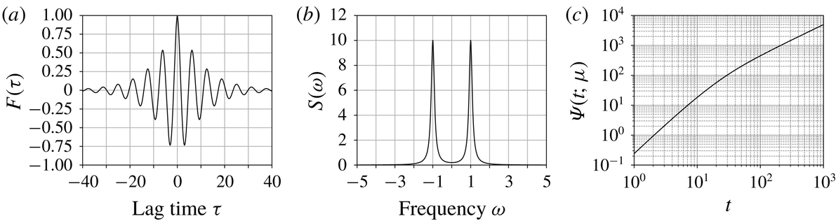
The function (2.13) represents a phase-modulating wave, with $\unicode[STIX]{x1D707}$ specifying the intensity of modulation. The parameter $\unicode[STIX]{x1D707}$ is interpreted physically as the reciprocal of the correlation length in the time domain (see figure 2 a) or the half-value width in the frequency domain (figure 2 b). Since $S(\unicode[STIX]{x1D714})$ and $K(\unicode[STIX]{x1D714},t)$ both include two terms with their spectrum peaks occurring at $\unicode[STIX]{x1D714}=\pm 1$ , if we ignore cross-multiplication terms, (2.6) can be calculated as

(2.16) $$\begin{eqnarray}\langle E\rangle \sim \frac{\unicode[STIX]{x1D716}^{2}t}{2\unicode[STIX]{x1D707}}+\frac{\unicode[STIX]{x1D716}^{2}}{2\unicode[STIX]{x1D707}^{2}}(\exp (-\unicode[STIX]{x1D707}t)-1)\equiv \unicode[STIX]{x1D716}^{2}\unicode[STIX]{x1D6F9}(t;\unicode[STIX]{x1D707}),\end{eqnarray}$$

where a new function $\unicode[STIX]{x1D6F9}(t;\unicode[STIX]{x1D707})$ is introduced. This function has two types of asymptotic forms:

(2.17) $$\begin{eqnarray}\unicode[STIX]{x1D6F9}(t;\unicode[STIX]{x1D707})=\frac{t}{2\unicode[STIX]{x1D707}}+\frac{\exp (-\unicode[STIX]{x1D707}t)-1}{2\unicode[STIX]{x1D707}^{2}}\sim \left\{\begin{array}{@{}ll@{}}\displaystyle \frac{t^{2}}{4}\quad & \text{for}~t\sim 0,\\ \displaystyle \frac{t}{2\unicode[STIX]{x1D707}}\quad & \text{for}~t\sim \infty .\end{array}\right.\end{eqnarray}$$

Notice that the power laws with respect to $t$ in (2.17) correspond to the prior two cases (2.10) and (2.11). Figure 2(c) presents plots of (2.17) on double-logarithmic axes, showing the transition of energy growth from the dynamic- to kinetic-type responses. Since the transition time can be scaled as $t\sim \unicode[STIX]{x1D707}^{-1}$ , let us define the ‘dynamic time range’ as $t\ll \unicode[STIX]{x1D707}^{-1}$ , and the ‘kinetic time range’ as $t\gg \unicode[STIX]{x1D707}^{-1}$ . It is interesting to note that conventional dynamic and kinetic ‘time scales’ are defined in terms of the amplitude of forcing, but the new concept of ‘time ranges’ are now introduced in terms of the spectrum width.

Figure 2.

(a) Autocorrelation function of the modulated sinusoidal function, as defined in (2.14). (b) Power spectrum of the modulated sinusoidal function, as defined in (2.15). (c) Double-logarithmic plot of function $\unicode[STIX]{x1D6F9}(t;\unicode[STIX]{x1D707})$ , which represents the time evolution of the energy expectation value of an oscillator in response to stochastic forcing (2.13). In all panels, $\unicode[STIX]{x1D707}=0.1$ is adopted.

The above result provides a criterion that determines the validity of (2.12). For the energy expectation value to be represented by (2.12), the measurement time $t$ must be longer than the correlation time of the forcing $\unicode[STIX]{x1D707}^{-1}$ . This property is rewarded in terms of the spectrum width. If we consider the integrand of the right-hand side of (2.6), the spectrum width of $K(\unicode[STIX]{x1D714},t)$ becomes narrower with time, whereas $S(\unicode[STIX]{x1D714})$ remains unchanged. For short times, $S(\unicode[STIX]{x1D714})$ is much narrower than $K(\unicode[STIX]{x1D714},t)$ , whereas over longer times the relation is reversed. The interchange occurs at $t\sim \unicode[STIX]{x1D707}^{-1}$ , corresponding to a transition from dynamic to kinetic time ranges. In the line spectrum limit $\unicode[STIX]{x1D707}\rightarrow 0$ , the transition time diverges to infinity, making the kinetic time range inaccessible. This is the simplest explanation as to why the expression (2.12) becomes invalid for a situation involving monochromatic forcing.

We can explain the difference between the two types of responses in an alternative way. In figure 3, grey curves show the numerically calculated sample paths of $E$ , excited by quasi-periodic forcing (2.13), whereas the black curve depicts their expectation value $\langle E\rangle$ . In the dynamic time range, almost all of the sample paths are close to the expectation value. In the kinetic time range, in contrast, each path shows random variations, deviating around the expectation value. From this property, it can be said that the transition from the dynamic to kinetic ranges corresponds to that from deterministic to stochastic ranges.

Figure 3.

Time evolution of the energy of the oscillator in response to stochastic forcing as specified in (2.1) and (2.13), depicted in a double-logarithmic graph. The grey curves are numerically obtained sample paths. The black curve represents their expectation value, which is defined in (2.16). The parameters are chosen as $\unicode[STIX]{x1D716}=1$ and $\unicode[STIX]{x1D707}=0.03$ .

3.1 Heuristic approach

Let us construct an asymptotic solution for (3.1) by first expanding $x$ in terms of $\unicode[STIX]{x1D716}$ :

(3.4) $$\begin{eqnarray}x=x_{0}+\unicode[STIX]{x1D716}x_{1}+\unicode[STIX]{x1D716}^{2}x_{2}+\cdots \,.\end{eqnarray}$$

The solutions up to the second order are as follows:

(3.5a ) $$\begin{eqnarray}\displaystyle & \displaystyle x_{0}=a\sin t, & \displaystyle\end{eqnarray}$$

(3.5b ) $$\begin{eqnarray}\displaystyle & \displaystyle x_{1}=-a\int _{0}^{t}\sin (t-t_{1})f(t_{1})\sin t_{1}\,\text{d}t_{1}, & \displaystyle\end{eqnarray}$$

(3.5c ) $$\begin{eqnarray}\displaystyle & \displaystyle x_{2}=a\int _{0}^{t}\sin (t-t_{1})f(t_{1})\int _{0}^{t_{1}}\sin (t_{1}-t_{2})f(t_{2})\sin t_{2}\,\text{d}t_{1}\,\text{d}t_{2}. & \displaystyle\end{eqnarray}$$

$f(t)$

$S(\unicode[STIX]{x1D714})$

$\langle E(t)\rangle =\langle x^{2}+{\dot{x}}^{2}\rangle /2$

(3.6a ) $$\begin{eqnarray}\displaystyle & \displaystyle \langle E\rangle =\frac{a^{2}}{2}+\frac{\unicode[STIX]{x1D716}^{2}a^{2}}{2\unicode[STIX]{x03C0}}\int _{-\infty }^{\infty }S(\unicode[STIX]{x1D714})K(\unicode[STIX]{x1D714},t)\,\text{d}\unicode[STIX]{x1D714}+O(\unicode[STIX]{x1D716}^{3}), & \displaystyle\end{eqnarray}$$

(3.6b ) $$\begin{eqnarray}\displaystyle & \displaystyle K(\unicode[STIX]{x1D714},t)=\frac{1-\cos ((\unicode[STIX]{x1D714}-2)t)}{2\unicode[STIX]{x1D714}(\unicode[STIX]{x1D714}-2)^{2}}-\frac{1-\cos ((\unicode[STIX]{x1D714}+2)t)}{2\unicode[STIX]{x1D714}(\unicode[STIX]{x1D714}+2)^{2}}. & \displaystyle\end{eqnarray}$$

$K(\unicode[STIX]{x1D714},t)$

$\unicode[STIX]{x1D714}=\pm 2$

Let us now assume that the variable coefficient is a phase-modulating wave,

(3.7) $$\begin{eqnarray}\displaystyle f(t)=\sqrt{2}\sin (2t+\sqrt{2\unicode[STIX]{x1D707}}W_{t}+\unicode[STIX]{x1D703}), & & \displaystyle\end{eqnarray}$$

and hence

(3.8) $$\begin{eqnarray}\displaystyle S(\unicode[STIX]{x1D714})=\frac{\unicode[STIX]{x1D707}}{(\unicode[STIX]{x1D714}+2)^{2}+\unicode[STIX]{x1D707}^{2}}+\frac{\unicode[STIX]{x1D707}}{(\unicode[STIX]{x1D714}-2)^{2}+\unicode[STIX]{x1D707}^{2}}. & & \displaystyle\end{eqnarray}$$

Ignoring the cross-multiplication terms and replacing the factors $\unicode[STIX]{x1D714}$ in the denominator of $K$ by the peak frequency $\pm 2$ , we can calculate (3.6) as

(3.9) $$\begin{eqnarray}\langle E\rangle =\frac{a^{2}}{2}+\frac{\unicode[STIX]{x1D716}^{2}a^{2}}{2}\left[\frac{t}{2\unicode[STIX]{x1D707}}+\frac{\exp (-\unicode[STIX]{x1D707}t)-1}{2\unicode[STIX]{x1D707}^{2}}\right]+O(\unicode[STIX]{x1D716}^{3}).\end{eqnarray}$$

The bracketed terms on the right-hand side of (3.9) are secular, which means that the resonant feedback to the energy of the oscillator accumulates with time and thus the solution (3.9) does not hold for large $t$ . To obtain a global solution, a singular perturbation approach is needed. Traditional singular perturbation methods such as described by Bender & Orszag (Reference Bender and Orszag1999) are not applicable to this problem; however, the renormalisation theory developed by Chen, Goldenfeld & Oono (Reference Chen, Goldenfeld and Oono1996) may be suitable. That is, we reconstruct a differential equation that is consistent with the regular perturbation solution (3.9) in $t\ll \unicode[STIX]{x1D716}^{-1}$ . In fact, this idea has already been employed in the derivation of (2.12). Although our method is not a strict mathematical procedure, the result agrees well with the numerical solutions and, more importantly, gives us basic insight into the applicability of the kinetic equation.

To make the problem simpler, the regular perturbation solution (3.9) is rewritten as

(3.10) $$\begin{eqnarray}\langle E(t)\rangle =\langle E(0)\rangle +\unicode[STIX]{x1D716}^{2}\unicode[STIX]{x1D6F9}(t;\unicode[STIX]{x1D707})\langle E(0)\rangle .\end{eqnarray}$$

We then consider two special cases.

Firstly, the function $\unicode[STIX]{x1D6F9}$ is evaluated in the dynamic time range. The energy expectation value (3.10) can then be approximated as

(3.11) $$\begin{eqnarray}\langle E(t)\rangle =\langle E(0)\rangle +\frac{\unicode[STIX]{x1D716}^{2}t^{2}}{4}\langle E(0)\rangle .\end{eqnarray}$$

The first and second derivatives of (3.11) at $t=0$ are written as

(3.12a,b ) $$\begin{eqnarray}\frac{\text{d}}{\text{d}t}\langle E\rangle =0,\quad \frac{\text{d}^{2}}{\text{d}t^{2}}\langle E\rangle =\frac{\unicode[STIX]{x1D716}^{2}}{2}\langle E\rangle .\end{eqnarray}$$

Again, solving the latter equation of (3.12) with the initial condition of the former, we obtain

(3.13) $$\begin{eqnarray}\langle E\rangle =\langle E(0)\rangle \cosh \left(\frac{\sqrt{2}\unicode[STIX]{x1D716}t}{2}\right).\end{eqnarray}$$

This result coincides with the basic solution (3.3).

Another situation occurs when $\unicode[STIX]{x1D6F9}$ is evaluated in the kinetic time range. In this case, equation (3.10) can be approximated as

(3.14) $$\begin{eqnarray}\langle E(t)\rangle =\langle E(0)\rangle +\frac{\unicode[STIX]{x1D716}^{2}t}{2\unicode[STIX]{x1D707}}\langle E(0)\rangle .\end{eqnarray}$$

The first derivative of (3.14) at $t=0$ is

(3.15) $$\begin{eqnarray}\frac{\text{d}}{\text{d}t}\langle E\rangle =\frac{\unicode[STIX]{x1D716}^{2}}{2\unicode[STIX]{x1D707}}\langle E\rangle ,\end{eqnarray}$$

which is solved as

(3.16) $$\begin{eqnarray}\langle E\rangle =\langle E(0)\rangle \exp \left(\frac{\unicode[STIX]{x1D716}^{2}t}{2\unicode[STIX]{x1D707}}\right).\end{eqnarray}$$

For the kinetic case, the growth rate is proportional to the square of $\unicode[STIX]{x1D716}$ and diverges in the narrow-band limit, $\unicode[STIX]{x1D707}\rightarrow 0$ , as mentioned in § 1.

The difference between (3.13) and (3.16) originates from the choice of a time range in which the resonance feedback is evaluated. How, then, should we adopt the time range? The answer depends on when the secular terms reach $O(1)$ . That is, if $\unicode[STIX]{x1D716}^{2}\unicode[STIX]{x1D6F9}(t)\sim O(1)$ occurs within the dynamic time range $t\ll \unicode[STIX]{x1D707}^{-1}$ , the approximation (3.11) is valid. If $\unicode[STIX]{x1D716}^{2}\unicode[STIX]{x1D6F9}(t)\sim O(1)$ occurs in the kinetic time range $t\gg \unicode[STIX]{x1D707}^{-1}$ , the approximation (3.14) becomes valid instead. Moreover, in the latter case, the time evolution of the energy expectation value is described by the first-order differential equation (3.15) in the same way as (2.12). The kinetic equation is generally derived in this way.

Figure 4.

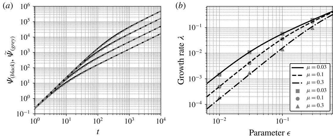
(a) Double-logarithmic plots of $\unicode[STIX]{x1D6F9}(t;\unicode[STIX]{x1D707})$ (solid black curves) and its approximate form $\tilde{\unicode[STIX]{x1D6F9}}(t;\unicode[STIX]{x1D707})$ (broken grey curves) for $\unicode[STIX]{x1D707}=0.01,0.03,0.1,0.3$ . The expressions are defined in (2.17) and (3.18). (b) Growth rates of the energy expectation value of the stochastically excited oscillator, as specified in (3.1) and (3.7). The black curves represent analytical solution (3.21), whereas the grey symbols represent experimental values. The numerical calculation was conducted 1000 times for each case using the fourth-order Runge–Kutta method with a time interval $\unicode[STIX]{x0394}t=0.03$ . The logarithm of the average energy is linearly fitted for $90\leqslant t\leqslant 450$ to estimate the growth rates.

We now seek a unified expression of the growth rate that is applicable to both the dynamic and kinetic cases. In the derivation of (3.12) and (3.15), we have replaced the secular terms in (3.10) by polynomial forms. Extending this idea, we consider a rational function

(3.17) $$\begin{eqnarray}\frac{t^{2}}{\unicode[STIX]{x1D6FC}+\unicode[STIX]{x1D6FD}t},\end{eqnarray}$$

which approaches $t^{2}/\unicode[STIX]{x1D6FC}$ as $t\rightarrow 0$ and $t/\unicode[STIX]{x1D6FD}$ as $t\rightarrow \infty$ . Choosing $\unicode[STIX]{x1D6FC}=4$ and $\unicode[STIX]{x1D6FD}=2\unicode[STIX]{x1D707}$ makes (2.17) and (3.17) asymptotically identical in both the short- and long-time limits. With this in mind, we define a new function,

(3.18) $$\begin{eqnarray}\tilde{\unicode[STIX]{x1D6F9}}(t;\unicode[STIX]{x1D707})=\frac{t^{2}}{4+2\unicode[STIX]{x1D707}t},\end{eqnarray}$$

and replace $\unicode[STIX]{x1D6F9}(t;\unicode[STIX]{x1D707})$ in (3.10) by $\tilde{\unicode[STIX]{x1D6F9}}(t;\unicode[STIX]{x1D707})$ . Figure 4(a) compares $\unicode[STIX]{x1D6F9}(t;\unicode[STIX]{x1D707})$ and $\tilde{\unicode[STIX]{x1D6F9}}(t;\unicode[STIX]{x1D707})$ in double-logarithmic plots. Close agreement between the two functions is promising regarding the validity of this approximation. Let us transform the equation $\langle E(t)\rangle =\langle E(0)\rangle +\unicode[STIX]{x1D716}^{2}\tilde{\unicode[STIX]{x1D6F9}}(t;\unicode[STIX]{x1D707})\langle E(0)\rangle$ into the following:

(3.19) $$\begin{eqnarray}(4+2\unicode[STIX]{x1D707}t)(\langle E(t)\rangle -\langle E(0)\rangle )-\unicode[STIX]{x1D716}^{2}t^{2}\langle E(0)\rangle =0.\end{eqnarray}$$

The second derivative of (3.19) at $t=0$ yields

(3.20) $$\begin{eqnarray}\frac{\text{d}^{2}}{\text{d}t^{2}}\langle E\rangle +\unicode[STIX]{x1D707}\frac{\text{d}}{\text{d}t}\langle E\rangle -\frac{\unicode[STIX]{x1D716}^{2}}{2}\langle E\rangle =0.\end{eqnarray}$$

The positive root of the characteristic equation of (3.20) is

(3.21) $$\begin{eqnarray}\unicode[STIX]{x1D706}=\frac{-\unicode[STIX]{x1D707}+\sqrt{\unicode[STIX]{x1D707}^{2}+2\unicode[STIX]{x1D716}^{2}}}{2}.\end{eqnarray}$$

The solution (3.21) has two asymptotic forms:

(3.22) $$\begin{eqnarray}\unicode[STIX]{x1D706}\sim \left\{\begin{array}{@{}ll@{}}\displaystyle \frac{\sqrt{2}\unicode[STIX]{x1D716}}{2}\quad & \text{for }\unicode[STIX]{x1D707}\ll \unicode[STIX]{x1D716},\\ \displaystyle \frac{\unicode[STIX]{x1D716}^{2}}{2\unicode[STIX]{x1D707}}\quad & \text{for }\unicode[STIX]{x1D707}\gg \unicode[STIX]{x1D716},\end{array}\right.\end{eqnarray}$$

in agreement with the dynamic and kinetic results, equations (3.13) and (3.16). Figure 4(b) compares the analytical solution (3.21) with the experimentally obtained growth rates. The unified solution (3.21) also agrees well with the results from direct numerical integrations.

3.2 Statistical theory

In § 3.1, the growth rate of stochastic parametric excitation was heuristically derived. Here, a more systematic consideration is presented based on a general statistical approach. Attention should be paid to the assumptions to be employed, as the validity of these is a central concern in the resonant interaction theory.

First, we introduce a complex variable $a=(x+\text{i}{\dot{x}})/\sqrt{2}$ , and rewrite (3.1) as

(3.23) $$\begin{eqnarray}\frac{\text{d}a}{\text{d}t}=-\text{i}a-\frac{\text{i}\unicode[STIX]{x1D716}}{2}fa-\frac{\text{i}\unicode[STIX]{x1D716}}{2}fa^{\dagger },\end{eqnarray}$$

where $^{\dagger }$ indicates the complex conjugate. Since the energy expectation value can be expressed as $\langle E\rangle =\langle a^{\dagger }a\rangle$ , equation (3.23) yields a simple energy equation,

(3.24) $$\begin{eqnarray}\frac{\text{d}}{\text{d}t}\langle E\rangle =-\unicode[STIX]{x1D716}\,\text{Im}\langle \,fa^{2}\rangle .\end{eqnarray}$$

This equation implies that the variation in energy expectation value is induced by the triple correlation of the complex variable $a$ and the forcing function $f$ . Now, we expand the complex variable as

(3.25) $$\begin{eqnarray}a(t)=a_{0}(t)+\unicode[STIX]{x1D716}a_{1}(t)+O(\unicode[STIX]{x1D716}^{2}).\end{eqnarray}$$

Substituting this into (3.23) gives the zero- and first-order equations:

(3.26a ) $$\begin{eqnarray}\displaystyle & \displaystyle \frac{\text{d}a_{0}}{\text{d}t}=-\text{i}a_{0}, & \displaystyle\end{eqnarray}$$

(3.26b ) $$\begin{eqnarray}\displaystyle & \displaystyle \frac{\text{d}a_{1}}{\text{d}t}=-\text{i}a_{1}-\frac{\text{i}\unicode[STIX]{x1D716}}{2}fa_{0}-\frac{\text{i}\unicode[STIX]{x1D716}}{2}fa_{0}^{\dagger }. & \displaystyle\end{eqnarray}$$

(3.27) $$\begin{eqnarray}a_{1}=-\frac{\text{i}\unicode[STIX]{x1D716}}{2}\int ^{t}\text{e}^{-\text{i}(t-t^{\prime })}(f(t^{\prime })a_{0}(t^{\prime })+f(t^{\prime })a_{0}^{\dagger }(t^{\prime }))\,\text{d}t^{\prime }.\end{eqnarray}$$

Substituting $a\sim a_{0}+\unicode[STIX]{x1D716}a_{1}$ together with (3.27) into (3.24) with the assumptions for the statistical properties,

(3.28a ) $$\begin{eqnarray}\displaystyle & \displaystyle \langle \,f(t)a_{0}(t)^{2}\rangle =0, & \displaystyle\end{eqnarray}$$

(3.28b ) $$\begin{eqnarray}\displaystyle & \displaystyle \langle \,f(t)f(t^{\prime })a_{0}(t)a_{0}(t^{\prime })\rangle =0, & \displaystyle\end{eqnarray}$$

(3.28c ) $$\begin{eqnarray}\displaystyle & \displaystyle \langle \,f(t)f(t^{\prime })a_{0}(t)a_{0}^{\dagger }(t^{\prime })\rangle =\langle \,f(t)f(t^{\prime })\rangle \langle a_{0}(t)a_{0}^{\dagger }(t^{\prime })\rangle , & \displaystyle\end{eqnarray}$$

(3.29) $$\begin{eqnarray}\frac{\text{d}}{\text{d}t}\langle E\rangle =\unicode[STIX]{x1D716}^{2}\,\text{Im}\int ^{t}\text{i}\text{e}^{-\text{i}(t-t^{\prime })}\langle \,f(t)f(t^{\prime })\rangle \langle a_{0}(t)a_{0}^{\dagger }(t^{\prime })\rangle \,\text{d}t^{\prime }.\end{eqnarray}$$

Taking into account $\langle \,f(t)f(t^{\prime })\rangle =F(t-t^{\prime })$ and making an additional assumption that $\langle a_{0}(t)a_{0}^{\dagger }(t^{\prime })\rangle \sim \text{e}^{-\text{i}(t-t^{\prime })}\langle E(t^{\prime })\rangle$ , which comes from (3.26a ), a closed equation

(3.30) $$\begin{eqnarray}\frac{\text{d}}{\text{d}t}\langle E\rangle =\unicode[STIX]{x1D716}^{2}\int ^{t}\cos (2(t-t^{\prime }))F(t-t^{\prime })\langle E(t^{\prime })\rangle \,\text{d}t^{\prime }\end{eqnarray}$$

is obtained. Conditions (3.28) argue that variations in the oscillator and the forcing function are statistically independent at their lowest order and their correlations can be evaluated from the perturbation terms. This corresponds to the classical Gaussian assumption (see § 4.1 for details) frequently made in turbulence theory.

In (3.30), the evolution of $\langle E\rangle$ depends on its earlier values. As we would like to discuss the long-term evolution of the system, the choice of initial condition at $t=0$ is inconvenient. Alternatively, we define the initial condition to be

(3.31) $$\begin{eqnarray}\langle E\rangle \rightarrow 0\quad \text{for }t\rightarrow -\infty .\end{eqnarray}$$

One may consider an additional Markovian approximation: to replace the energy expectation value $\langle E(t^{\prime })\rangle$ in the integrand of (3.30) by the present value $\langle E(t)\rangle$ . This allows the time integration on the right-hand side to be performed without solving the differential equation. This coincides with the procedure in the derivation of (2.12), which again breaks down if the correlation function $F(\unicode[STIX]{x1D70F})$ involves a pure sinusoidal function. To avoid this problem, we now directly solve (3.30), by assuming only an exponential function $\langle E(t)\rangle =\text{e}^{\unicode[STIX]{x1D706}t}$ as its solution. Transforming the correlation function $F(\unicode[STIX]{x1D70F})$ into the power spectrum $S(\unicode[STIX]{x1D714})$ and integrating the right-hand side of (3.30) from $-\infty$ to $0$ , we obtain the characteristic equation

(3.32) $$\begin{eqnarray}\unicode[STIX]{x1D706}=\frac{\unicode[STIX]{x1D716}^{2}}{2\unicode[STIX]{x03C0}}\int _{-\infty }^{\infty }S(\unicode[STIX]{x1D714})\left(\frac{\unicode[STIX]{x1D706}}{2((\unicode[STIX]{x1D714}+2)^{2}+\unicode[STIX]{x1D706}^{2})}+\frac{\unicode[STIX]{x1D706}}{2((\unicode[STIX]{x1D714}-2)^{2}+\unicode[STIX]{x1D706}^{2})}\right)\text{d}\unicode[STIX]{x1D714},\end{eqnarray}$$

which determines the growth rate $\unicode[STIX]{x1D706}$ in response to a given power spectrum $S$ .

A special choice of $S$ for a phase-modulating wave, (3.8), reduces (3.32) to a simple algebraic equation,

(3.33) $$\begin{eqnarray}\unicode[STIX]{x1D706}=\frac{\unicode[STIX]{x1D716}^{2}}{2(\unicode[STIX]{x1D706}+\unicode[STIX]{x1D707})},\end{eqnarray}$$

where trivial cross-multiplication terms are neglected. The positive root of (3.33) is given as $\unicode[STIX]{x1D706}=(-\unicode[STIX]{x1D707}+\sqrt{\unicode[STIX]{x1D707}^{2}+2\unicode[STIX]{x1D716}^{2}})/2$ . This is equivalent to the result of § 3.1, that is, (3.21).

Although the heuristic method in § 3.1 and the statistical theory introduced here both produce the same result in the current example, the latter is a more useful methodological approach than the former. The difference between them can be clearly seen when we consider the effect of detuning. If the central frequency of the external function in (3.1) deviates slightly from twice the natural frequency of the system as

(3.34) $$\begin{eqnarray}f=\sqrt{2}\sin ((2+\unicode[STIX]{x1D702})t+\sqrt{2\unicode[STIX]{x1D707}}W_{t}+\unicode[STIX]{x1D703})\quad (\unicode[STIX]{x1D702}\ll 1),\end{eqnarray}$$

the energy growth moderates as $\unicode[STIX]{x1D702}$ increases. The heuristic method fails to cope with this problem. On the other hand, the characteristic equation (3.32) derived from the statistical theory in this case reduces to

(3.35) $$\begin{eqnarray}\unicode[STIX]{x1D706}=\frac{\unicode[STIX]{x1D716}^{2}(\unicode[STIX]{x1D706}+\unicode[STIX]{x1D707})}{2(\unicode[STIX]{x1D706}+\unicode[STIX]{x1D707})^{2}+\unicode[STIX]{x1D702}^{2}}.\end{eqnarray}$$

This is a reasonable result since the positive root of (3.35) coincides with the classical solution (appendix B) in the limit of $\unicode[STIX]{x1D707}\rightarrow 0$ .

4.1 Statistical description of wave–wave interaction

Wave motions are generally described by partial differential equations in which all the variables are defined as functions of both spatial and temporal coordinates. To discuss the wave–wave interactions, however, it is rather convenient to take the Fourier transform such that each spatial coordinate is replaced by the corresponding wavenumber. As a result, the governing equations are transformed into an integro-differential equation. Moreover, in many cases, a conservative wave system can be represented in a simple Hamiltonian form, and a common procedure can be utilised to derive a statistical equation that describes the energy transfer in wavevector space (see Zakharov et al. Reference Zakharov, L’vov and Falkovich1992). The most standard model for a three-wave system in $d$ -dimensional space is described by the Hamiltonian

(4.1a ) $$\begin{eqnarray}\displaystyle & \displaystyle {\mathcal{H}}={\mathcal{H}}_{2}+\unicode[STIX]{x1D716}{\mathcal{H}}_{3}, & \displaystyle\end{eqnarray}$$

(4.1b ) $$\begin{eqnarray}\displaystyle & \displaystyle {\mathcal{H}}_{2}=\int \unicode[STIX]{x1D714}(\boldsymbol{k})a^{\dagger }(\boldsymbol{k})a(\boldsymbol{k})\,\text{d}\boldsymbol{k}, & \displaystyle\end{eqnarray}$$

(4.1c ) $$\begin{eqnarray}\displaystyle {\mathcal{H}}_{3} & = & \displaystyle \int \left\{\frac{1}{2}V(\boldsymbol{k}_{1},\boldsymbol{k}_{2},\boldsymbol{k}_{3})a^{\dagger }(\boldsymbol{k}_{1})a(\boldsymbol{k}_{2})a(\boldsymbol{k}_{3})\unicode[STIX]{x1D6FF}(\boldsymbol{k}_{1}-\boldsymbol{k}_{2}-\boldsymbol{k}_{3})\right.\nonumber\\ \displaystyle & & \displaystyle \left.+\,\frac{1}{6}U(\boldsymbol{k}_{1},\boldsymbol{k}_{2},\boldsymbol{k}_{3})a(\boldsymbol{k}_{1})a(\boldsymbol{k}_{2})a(\boldsymbol{k}_{3})\unicode[STIX]{x1D6FF}(\boldsymbol{k}_{1}+\boldsymbol{k}_{2}+\boldsymbol{k}_{3})\right\}\text{d}\boldsymbol{k}_{1}\,\text{d}\boldsymbol{k}_{2}\,\text{d}\boldsymbol{k}_{3}+\text{c.c.},\quad\end{eqnarray}$$

(4.2) $$\begin{eqnarray}\text{i}\frac{\unicode[STIX]{x2202}a}{\unicode[STIX]{x2202}t}=\frac{\unicode[STIX]{x1D6FF}{\mathcal{H}}}{\unicode[STIX]{x1D6FF}a^{\dagger }},\end{eqnarray}$$

where $a(\boldsymbol{k},t)$ is a complex variable defined as a function of wavevector $\boldsymbol{k}\in \mathbb{R}^{d}$ ,  $\unicode[STIX]{x1D6FF}(\boldsymbol{k})$ is the $d$ -dimensional delta function, coefficients $\unicode[STIX]{x1D714}(\boldsymbol{k})$ ,  $V(\boldsymbol{k}_{1},\boldsymbol{k}_{2},\boldsymbol{k}_{3})$ and $U(\boldsymbol{k}_{1},\boldsymbol{k}_{2},\boldsymbol{k}_{3})$ are functions constant in time, $\unicode[STIX]{x1D716}$ is a constant parameter, c.c. denotes the complex conjugate of the previous terms, and integration is performed over the whole wavenumber space. Without loss of generality, we may assume the symmetry of the arguments of the coefficients: $V(\boldsymbol{k}_{1},\boldsymbol{k}_{2},\boldsymbol{k}_{3})=V(\boldsymbol{k}_{1},\boldsymbol{k}_{3},\boldsymbol{k}_{2})$ and $U$ does not change under any permutation of the arguments. We further assume that $\unicode[STIX]{x1D714}(\boldsymbol{k})>0$ holds almost everywhere in $\mathbb{R}^{d}$ , which assures the positivity of the Hamiltonian ${\mathcal{H}}$ in the asymptotic limit $\unicode[STIX]{x1D716}\rightarrow 0$ . Appendix C briefly describes the formulation of this model for the case of rotating long internal waves.

Variable $a(\boldsymbol{k},t)$ specifies the amplitude and phase of the wavevector $\boldsymbol{k}$ component; it is translated to the real domain, $\boldsymbol{r}\in \mathbb{R}^{d}$ , by the inverse Fourier transform, $(2\unicode[STIX]{x03C0})^{-d/2}\int a(\boldsymbol{k},t)\text{e}^{\text{i}\boldsymbol{k}\boldsymbol{\cdot }\boldsymbol{r}}\,\text{d}\boldsymbol{k}$ . Expanding the functional derivative of (4.2) leads to an integro-differential equation:

(4.3) $$\begin{eqnarray}\text{i}\frac{\unicode[STIX]{x2202}a_{1}}{\unicode[STIX]{x2202}t}=\unicode[STIX]{x1D714}_{1}a_{1}+\unicode[STIX]{x1D716}\int \left(\frac{1}{2}V_{123}a_{2}a_{3}\unicode[STIX]{x1D6FF}_{1-2-3}+V_{213}^{\dagger }a_{2}a_{3}^{\dagger }\unicode[STIX]{x1D6FF}_{2-1-3}+\frac{1}{2}U_{123}^{\dagger }a_{2}^{\dagger }a_{3}^{\dagger }\unicode[STIX]{x1D6FF}_{1+2+3}\right)\text{d}\boldsymbol{k}_{23},\end{eqnarray}$$

where, for conciseness, subscripts are used to represent the arguments of a variable; specifically, $a_{1}=a(\boldsymbol{k}_{1},t),~\unicode[STIX]{x1D714}_{1}=\unicode[STIX]{x1D714}(\boldsymbol{k}_{1}),~V_{123}=V(\boldsymbol{k}_{1},\boldsymbol{k}_{2},\boldsymbol{k}_{3}),~U_{123}=U(\boldsymbol{k}_{1},\boldsymbol{k}_{2},\boldsymbol{k}_{3})$ and $\unicode[STIX]{x1D6FF}_{1-2-3}=\unicode[STIX]{x1D6FF}(\boldsymbol{k}_{1}-\boldsymbol{k}_{2}-\boldsymbol{k}_{3})$ . From (4.3), one may understand that $\unicode[STIX]{x1D714}(\boldsymbol{k})$ represents the linear dispersion relation, $V(\boldsymbol{k}_{1},\boldsymbol{k}_{2},\boldsymbol{k}_{3})$ and $U(\boldsymbol{k}_{1},\boldsymbol{k}_{2},\boldsymbol{k}_{3})$ represent the nonlinear coupling coefficients for triad interaction, and $\unicode[STIX]{x1D716}$ specifies the intensity of the nonlinear interaction. We shall regard $\unicode[STIX]{x1D716}$ to be small, that is, the nonlinearity is sufficiently weak.

In the following, we will construct a statistical model to describe the nonlinear energy transfer among waves. First of all, as in the previous sections, let us introduce the notation $\langle \cdot \rangle$ to specify the ensemble average. Then, we assume the spatial homogeneity of the system in a statistical sense; that is, any kind of statistical quantity is invariant with respect to the coordinate change in the real domain, $\boldsymbol{r}\rightarrow \boldsymbol{r}+\boldsymbol{r}^{\prime }$ . Since this transformation changes the $m$ th moment of $a$ and $a^{\dagger }$ as

(4.4) $$\begin{eqnarray}\langle a_{1}\ldots a_{l}a_{l+1}^{\dagger }\ldots a_{m}^{\dagger }\rangle \rightarrow \langle a_{1}\ldots a_{l}a_{l+1}^{\dagger }\ldots a_{m}^{\dagger }\rangle \text{e}^{-\text{i}(\boldsymbol{k}_{1}+\cdots +\boldsymbol{k}_{l}-\boldsymbol{k}_{l+1}-\cdots -\boldsymbol{k}_{m})\boldsymbol{\cdot }\boldsymbol{r}^{\prime }},\end{eqnarray}$$

it can become non-zero only if $\boldsymbol{k}_{1}+\cdots +\boldsymbol{k}_{l}-\boldsymbol{k}_{l+1}-\cdots -\boldsymbol{k}_{m}=0$ is satisfied. This condition allows the second- and third-order correlation functions (here we omit $\langle a_{1}a_{2}\rangle$ since it will not appear in the following discussion) to be represented as

(4.5a ) $$\begin{eqnarray}\displaystyle & \displaystyle \langle a^{\dagger }(\boldsymbol{k}_{1},t)a(\boldsymbol{k}_{2},t)\rangle =n(\boldsymbol{k}_{1},t)\unicode[STIX]{x1D6FF}(\boldsymbol{k}_{1}-\boldsymbol{k}_{2}), & \displaystyle\end{eqnarray}$$

(4.5b ) $$\begin{eqnarray}\displaystyle & \displaystyle \langle a^{\dagger }(\boldsymbol{k}_{1},t)a(\boldsymbol{k}_{2},t)a(\boldsymbol{k}_{3},t)\rangle =J(\boldsymbol{k}_{1},\boldsymbol{k}_{2},\boldsymbol{k}_{3},t)\unicode[STIX]{x1D6FF}(\boldsymbol{k}_{1}-\boldsymbol{k}_{2}-\boldsymbol{k}_{3}), & \displaystyle\end{eqnarray}$$

(4.5c ) $$\begin{eqnarray}\displaystyle & \displaystyle \langle a(\boldsymbol{k}_{1},t)a(\boldsymbol{k}_{2},t)a(\boldsymbol{k}_{3},t)\rangle =K(\boldsymbol{k}_{1},\boldsymbol{k}_{2},\boldsymbol{k}_{3},t)\unicode[STIX]{x1D6FF}(\boldsymbol{k}_{1}+\boldsymbol{k}_{2}+\boldsymbol{k}_{3}). & \displaystyle\end{eqnarray}$$

$n,~J,~K$

$n_{1}=n(\boldsymbol{k}_{1},t),~J_{123}=J(\boldsymbol{k}_{1},\boldsymbol{k}_{2},\boldsymbol{k}_{3},t)$

$K_{123}=K(\boldsymbol{k}_{1},\boldsymbol{k}_{2},\boldsymbol{k}_{3},t)$

$a_{1^{\prime }}^{\dagger }$

$\boldsymbol{k}_{1^{\prime }}$

$n$

(4.6) $$\begin{eqnarray}\displaystyle \frac{\unicode[STIX]{x2202}n_{1}}{\unicode[STIX]{x2202}t}=\unicode[STIX]{x1D716}\,\text{Im}\int (V_{123}J_{123}\unicode[STIX]{x1D6FF}_{1-2-3}-2V_{213}J_{213}\unicode[STIX]{x1D6FF}_{2-1-3}-U_{123}K_{123}\unicode[STIX]{x1D6FF}_{1+2+3})\,\text{d}\boldsymbol{k}_{23}. & & \displaystyle\end{eqnarray}$$

To calculate this equation, we need to evaluate the third-order correlation functions $J$ and $K$ in terms of the second-order correlation function $n$ . This closure problem can be solved under the weak nonlinearity condition and the statistical assumptions.

Assuming that the nonlinear parameter $\unicode[STIX]{x1D716}$ is small, let us expand the variable $a$ as

(4.7) $$\begin{eqnarray}a=a^{0}+\unicode[STIX]{x1D716}a^{1}+\cdots \,,\end{eqnarray}$$

where the superscripts denote the order of perturbation. Substituting (4.7) into (4.3) and evaluating the $O(1)$ and $O(\unicode[STIX]{x1D716})$ terms, respectively, we readily obtain the leading-order solution,

(4.8) $$\begin{eqnarray}\displaystyle a^{0}(\boldsymbol{k},t)=a^{0}(\boldsymbol{k},t^{\prime })\text{e}^{-\text{i}\unicode[STIX]{x1D714}(\boldsymbol{k})(t-t^{\prime })}, & & \displaystyle\end{eqnarray}$$

where the ‘initial’ time $t^{\prime }$ can be arbitrarily chosen, and the first-order solution,

(4.9) $$\begin{eqnarray}\displaystyle a_{1}^{1} & = & \displaystyle -\text{i}\int ^{t}\text{e}^{-\text{i}\unicode[STIX]{x1D714}_{1}(t-t^{\prime })}\int \left(\frac{1}{2}V_{123}a_{2}^{0}(t^{\prime })a_{3}^{0}(t^{\prime })\unicode[STIX]{x1D6FF}_{1-2-3}\right.\nonumber\\ \displaystyle & & \displaystyle \left.+\,V_{213}^{\dagger }a_{2}^{0}(t^{\prime })a_{3}^{0\dagger }(t^{\prime })\unicode[STIX]{x1D6FF}_{2-1-3}+\frac{1}{2}U_{123}^{\dagger }a_{2}^{0\dagger }(t^{\prime })a_{3}^{0\dagger }(t^{\prime })\unicode[STIX]{x1D6FF}_{1+2+3}\right)\text{d}\boldsymbol{k}_{23}\,\text{d}t^{\prime }.\end{eqnarray}$$

Next we employ the statistical assumptions for the different-time correlations of the leading-order variable $a^{0}$ . (The assumption used here is referred to as the random phase and amplitude (RPA) field (Nazarenko Reference Nazarenko2011), a generalised version of the classical Gaussian field. Since the phase-modulated wave adopted in this study, such as (2.13), is not Gaussian, RPA is more suitable in the present context.) Although a similar assumption has already been introduced in § 3.2, here we explain it more precisely. Let us separate $a^{0}$ into its amplitude and phase:

(4.10) $$\begin{eqnarray}\displaystyle a^{0}(\boldsymbol{k},t)=\unicode[STIX]{x1D6FC}(\boldsymbol{k},t)\text{e}^{\text{i}\unicode[STIX]{x1D703}(\boldsymbol{k},t)}. & & \displaystyle\end{eqnarray}$$

Then we regard $\unicode[STIX]{x1D6FC}(\boldsymbol{k},t)$ and $\unicode[STIX]{x1D703}(\boldsymbol{k},t)$ as statistically independent of all $\boldsymbol{k}\in \mathbb{R}^{d}$ with $\unicode[STIX]{x1D703}(\boldsymbol{k},t)$ distributed uniformly from $0$ to $2\unicode[STIX]{x03C0}$ . This assumption makes odd-order correlations trivially zero. Besides, an even-order correlation can become non-zero only if $a$ and $a^{\dagger }$ appear the same times in it; i.e. if $m=2l$ holds in $\langle a_{1}^{0}\ldots a_{l}^{0}a_{l+1}^{0\dagger }\ldots a_{m}^{0\dagger }\rangle$ . With use of (4.8), the non-trivial second-order correlation is written as

(4.11) $$\begin{eqnarray}\displaystyle \langle a_{1}^{0}(t)a_{2}^{0\dagger }(t^{\prime })\rangle =n_{1}(t^{\prime })\unicode[STIX]{x1D6FF}(\boldsymbol{k}_{1}-\boldsymbol{k}_{2})\text{e}^{-\text{i}\unicode[STIX]{x1D714}_{1}(t-t^{\prime })}. & & \displaystyle\end{eqnarray}$$

The non-trivial fourth-order correlation is evaluated by using the second-order correlations as

(4.12) $$\begin{eqnarray}\displaystyle \langle a_{1}^{0}a_{2}^{0}a_{3}^{0\dagger }a_{4}^{0\dagger }\rangle =\langle a_{1}^{0}a_{3}^{0\dagger }\rangle \langle a_{2}^{0}a_{4}^{0\dagger }\rangle +\langle a_{1}^{0}a_{4}^{0\dagger }\rangle \langle a_{2}^{0}a_{3}^{0\dagger }\rangle , & & \displaystyle\end{eqnarray}$$

except for the special case of $\boldsymbol{k}_{1}=\boldsymbol{k}_{2}=\boldsymbol{k}_{3}=\boldsymbol{k}_{4}$ , which we neglect since it will not contribute to resonant interaction in dispersive wave systems. We substitute (4.7) together with (4.9) into the left-hand sides of (4.5b ) and (4.5c ), evaluate the correlation terms using (4.11) and (4.12), perform the wavenumber integrations, and omit the delta functions on both sides, to obtain

(4.13a ) $$\begin{eqnarray}\displaystyle & \displaystyle J_{123}=\text{i}\unicode[STIX]{x1D716}\int ^{t}\text{e}^{\text{i}(\unicode[STIX]{x1D714}_{1}-\unicode[STIX]{x1D714}_{2}-\unicode[STIX]{x1D714}_{3})(t-t^{\prime })}V_{123}^{\dagger }(n_{2}(t^{\prime })n_{3}(t^{\prime })-n_{1}(t^{\prime })n_{3}(t^{\prime })-n_{1}(t^{\prime })n_{2}(t^{\prime }))\,\text{d}t^{\prime },\qquad & \displaystyle\end{eqnarray}$$

(4.13b ) $$\begin{eqnarray}\displaystyle & \displaystyle K_{123}=-\frac{\text{i}\unicode[STIX]{x1D716}}{2}\int ^{t}\text{e}^{-\text{i}(\unicode[STIX]{x1D714}_{1}+\unicode[STIX]{x1D714}_{2}+\unicode[STIX]{x1D714}_{3})(t-t^{\prime })}U_{123}^{\dagger }(n_{1}(t^{\prime })n_{2}(t^{\prime })+n_{1}(t^{\prime })n_{3}(t^{\prime })+n_{2}(t^{\prime })n_{3}(t^{\prime }))\,\text{d}t^{\prime }. & \displaystyle \nonumber\\ \displaystyle & & \displaystyle\end{eqnarray}$$

$J$

$K$

$n$

$n$

If we replace the past value of the second-order correlation $n(t^{\prime })$ in (4.13) by its present value $n(t)$ , i.e. using the Markovian approximation, and then integrate (4.13) from $-\infty$ to $t$ , (4.6) reduces to the usual kinetic equation,

(4.14) $$\begin{eqnarray}\displaystyle \frac{\unicode[STIX]{x2202}n_{1}}{\unicode[STIX]{x2202}t} & = & \displaystyle \unicode[STIX]{x1D716}^{2}\unicode[STIX]{x03C0}\int \{|V_{123}|^{2}(n_{2}n_{3}-n_{1}n_{3}-n_{1}n_{2})\unicode[STIX]{x1D6FF}(\boldsymbol{k}_{1}-\boldsymbol{k}_{2}-\boldsymbol{k}_{3})\unicode[STIX]{x1D6FF}(\unicode[STIX]{x1D714}_{1}-\unicode[STIX]{x1D714}_{2}-\unicode[STIX]{x1D714}_{3})\nonumber\\ \displaystyle & & \displaystyle -\,2|V_{213}|^{2}(n_{1}n_{3}-n_{1}n_{2}-n_{2}n_{3})\unicode[STIX]{x1D6FF}(\boldsymbol{k}_{2}-\boldsymbol{k}_{1}-\boldsymbol{k}_{3})\unicode[STIX]{x1D6FF}(\unicode[STIX]{x1D714}_{2}-\unicode[STIX]{x1D714}_{1}-\unicode[STIX]{x1D714}_{3})\}\,\text{d}\boldsymbol{k}_{23}.\qquad\end{eqnarray}$$

(Here, we assume that $\unicode[STIX]{x1D714}_{1}+\unicode[STIX]{x1D714}_{2}+\unicode[STIX]{x1D714}_{3}$ never becomes equal to zero, so that the terms involving $U$ trivially vanish.) However, this procedure is valid only in a steady state. For an unsteady process, especially for the instability problem, the Markovian approximation might not be valid. In such a case, a set of equations (4.6) and (4.13) is a more appropriate statistical model since it takes into account the ‘hysteresis’ of the spectrum.

4.2 Stability analysis

We now analyse the stability of a modulating wave train using the statistical equation, (4.6) and (4.13). To simplify the problem, some presumptions are made:

1. (i) The action density is decomposed into separable background and infinitesimal disturbance components, $n=N_{B}+n^{\prime }$ . The background spectrum $N_{B}(\boldsymbol{k})$ is idealised as a strict stationary solution of the basic statistical equation, i.e. $N_{B}(\boldsymbol{k})$ is a solution of the kinetic equation (4.14) with $\unicode[STIX]{x2202}n/\unicode[STIX]{x2202}t=0$ .

2. (ii) The background spectrum $N_{B}(\boldsymbol{k})$ represents a modulating wave train with the carrier wavevector $\boldsymbol{k}_{B}$ . Therefore, $N_{B}(\boldsymbol{k})$ vanishes except in the vicinity of a sharp peak at $\boldsymbol{k}_{B}$ .

3. (iii) The disturbance spectrum $n^{\prime }(\boldsymbol{k})$ is enhanced through the resonant or near-resonant interactions with the background components. Therefore, $n^{\prime }(\boldsymbol{k})$ vanishes except in the vicinity of the $(d-1)$ -dimensional manifold where wavevectors $\boldsymbol{k}_{1}$ and $\boldsymbol{k}_{2}$ satisfy the perfect resonance conditions:

   (4.15) $$\begin{eqnarray}\displaystyle \boldsymbol{k}_{1}+\boldsymbol{k}_{2}-\boldsymbol{k}_{B}=0,\quad \unicode[STIX]{x1D714}(\boldsymbol{k}_{1})+\unicode[STIX]{x1D714}(\boldsymbol{k}_{2})-\unicode[STIX]{x1D714}(\boldsymbol{k}_{B})=0. & & \displaystyle\end{eqnarray}$$

4. (iv) Terms that do not cause resonance, especially all the terms with the coefficient $U$ , are ignored.

Consequently, combining (4.6) and (4.13), we can obtain the approximate evolution equation for $n^{\prime }$ as

(4.16) $$\begin{eqnarray}\displaystyle \frac{\unicode[STIX]{x2202}n^{\prime }(\boldsymbol{k}_{\unicode[STIX]{x1D6FC}},t)}{\unicode[STIX]{x2202}t} & = & \displaystyle 2\unicode[STIX]{x1D716}^{2}\,\text{Re}\int \text{d}\boldsymbol{k}\,\text{d}\boldsymbol{k}_{\unicode[STIX]{x1D6FD}}\,\unicode[STIX]{x1D6FF}(-\boldsymbol{k}_{\unicode[STIX]{x1D6FC}}+\boldsymbol{k}-\boldsymbol{k}_{\unicode[STIX]{x1D6FD}})\nonumber\\ \displaystyle & & \displaystyle \times \int ^{t}\text{d}t^{\prime }\,\{\text{e}^{\text{i}(\unicode[STIX]{x1D714}(\boldsymbol{k}_{\unicode[STIX]{x1D6FC}})-\unicode[STIX]{x1D714}(\boldsymbol{k})+\unicode[STIX]{x1D714}(\boldsymbol{k}_{\unicode[STIX]{x1D6FD}}))(t-t^{\prime })}|V(\boldsymbol{k},\boldsymbol{k}_{\unicode[STIX]{x1D6FC}},\boldsymbol{k}_{\unicode[STIX]{x1D6FD}})|^{2}N_{B}(\boldsymbol{k})n^{\prime }(\boldsymbol{k}_{\unicode[STIX]{x1D6FD}},t^{\prime })\nonumber\\ \displaystyle & & \displaystyle +\,\text{e}^{\text{i}(\unicode[STIX]{x1D714}(\boldsymbol{k}_{\unicode[STIX]{x1D6FC}})-\unicode[STIX]{x1D714}(\boldsymbol{k})+\unicode[STIX]{x1D714}(\boldsymbol{k}_{\unicode[STIX]{x1D6FD}}))(t-t^{\prime })}|V(\boldsymbol{k},\boldsymbol{k}_{\unicode[STIX]{x1D6FC}},\boldsymbol{k}_{\unicode[STIX]{x1D6FD}})|^{2}N_{B}(\boldsymbol{k})n^{\prime }(\boldsymbol{k}_{\unicode[STIX]{x1D6FC}},t^{\prime })\}.\end{eqnarray}$$

Supposing the solution of (4.16) to be an exponential function $n^{\prime }=N(\boldsymbol{k})\text{e}^{\unicode[STIX]{x1D706}t}$ , integration of the right-hand side with respect to $t^{\prime }$ from $-\infty$ to $0$ yields a nonlinear eigenvalue problem,

(4.17) $$\begin{eqnarray}\displaystyle \unicode[STIX]{x1D706}N(\boldsymbol{k}_{\unicode[STIX]{x1D6FC}}) & = & \displaystyle \unicode[STIX]{x1D716}^{2}\int \text{d}\boldsymbol{k}\,\text{d}\boldsymbol{k}_{\unicode[STIX]{x1D6FD}}\,\unicode[STIX]{x1D6FF}(-\boldsymbol{k}_{\unicode[STIX]{x1D6FC}}+\boldsymbol{k}-\boldsymbol{k}_{\unicode[STIX]{x1D6FD}})\nonumber\\ \displaystyle & & \displaystyle \times \{\unicode[STIX]{x1D6F7}(\unicode[STIX]{x1D714}(\boldsymbol{k}_{\unicode[STIX]{x1D6FC}})-\unicode[STIX]{x1D714}(\boldsymbol{k})+\unicode[STIX]{x1D714}(\boldsymbol{k}_{\unicode[STIX]{x1D6FD}}),\unicode[STIX]{x1D706})|V(\boldsymbol{k},\boldsymbol{k}_{\unicode[STIX]{x1D6FC}},\boldsymbol{k}_{\unicode[STIX]{x1D6FD}})|^{2}N_{B}(\boldsymbol{k})N(\boldsymbol{k}_{\unicode[STIX]{x1D6FD}})\nonumber\\ \displaystyle & & \displaystyle +\,\unicode[STIX]{x1D6F7}(\unicode[STIX]{x1D714}(\boldsymbol{k}_{\unicode[STIX]{x1D6FC}})-\unicode[STIX]{x1D714}(\boldsymbol{k})+\unicode[STIX]{x1D714}(\boldsymbol{k}_{\unicode[STIX]{x1D6FD}}),\unicode[STIX]{x1D706})|V(\boldsymbol{k},\boldsymbol{k}_{\unicode[STIX]{x1D6FC}},\boldsymbol{k}_{\unicode[STIX]{x1D6FD}})|^{2}N_{B}(\boldsymbol{k})N(\boldsymbol{k}_{\unicode[STIX]{x1D6FC}})\},\end{eqnarray}$$

with an associated transfer function,

(4.18) $$\begin{eqnarray}\unicode[STIX]{x1D6F7}(\unicode[STIX]{x1D714},\unicode[STIX]{x1D706})\equiv \frac{2\unicode[STIX]{x1D706}}{(\unicode[STIX]{x1D714}^{2}+\unicode[STIX]{x1D706}^{2})}.\end{eqnarray}$$

Equation (4.17) is a kind of self-consistent equation; the ‘renormalised’ transfer function $\unicode[STIX]{x1D6F7}$ contains an unknown parameter $\unicode[STIX]{x1D706}$ that is to be determined. It is worth noting that, in the limit of $\unicode[STIX]{x1D706}\rightarrow 0$ ,  $\unicode[STIX]{x1D6F7}(\unicode[STIX]{x1D714},\unicode[STIX]{x1D706})$ approaches $2\unicode[STIX]{x03C0}\unicode[STIX]{x1D6FF}(\unicode[STIX]{x1D714})$ and hence the problem reduces to that obtained from the usual kinetic equation. In the following, we discuss the solution of (4.17) with finite $\unicode[STIX]{x1D706}$ using some simplifications.

4.3 One-dimensional case

Although interaction among oceanic internal waves is a three-dimensional process, we make the discussion simpler by first considering a one-dimensional problem $(d=1)$ . In this model, both the analytical and numerical solutions for (4.17) are accessible. Attention should be directed to the additional factor from the case in § 3, namely, the shape of the disturbance spectrum $N(\boldsymbol{k})$ , which corresponds to the eigenfunction of the unstable mode.

Let us write the solution of the resonant condition (4.15) as $k_{1}=k_{1}^{c},~k_{2}=k_{2}^{c}$ and decompose the disturbance spectrum as $N(k)=N_{1}(k)+N_{2}(k)$ with $N_{1}$ and $N_{2}$ concentrated near $k_{1}^{c}$ and $k_{2}^{c}$ , respectively. We then redefine the wavenumber coordinates as the deviations from $k_{B},~k_{1}^{c},~k_{2}^{c}$ , i.e. $k=k_{B}+k^{\prime }$ and $(k_{\unicode[STIX]{x1D6FC}},k_{\unicode[STIX]{x1D6FD}})=(k_{1}^{c},k_{2}^{c})+(k_{1}^{\prime },k_{2}^{\prime })$ or $(k_{\unicode[STIX]{x1D6FC}},k_{\unicode[STIX]{x1D6FD}})=(k_{2}^{c},k_{1}^{c})+(k_{2}^{\prime },k_{1}^{\prime })$ . The first-order truncation of a Taylor expansion in the denominator of the transfer function in (4.17) yields

(4.19a ) $$\begin{eqnarray}\displaystyle \unicode[STIX]{x1D6F7}(\unicode[STIX]{x1D714}(k_{1})+\unicode[STIX]{x1D714}(k_{2})-\unicode[STIX]{x1D714}(k),\unicode[STIX]{x1D706})\sim \frac{2\unicode[STIX]{x1D706}}{((c-c_{1})k^{\prime }+(c_{1}-c_{2})k_{2}^{\prime })^{2}+\unicode[STIX]{x1D706}^{2}} & & \displaystyle\end{eqnarray}$$

(4.19b ) $$\begin{eqnarray}\displaystyle =\frac{2\unicode[STIX]{x1D706}}{((c-c_{2})k^{\prime }+(c_{2}-c_{1})k_{1}^{\prime })^{2}+\unicode[STIX]{x1D706}^{2}}, & & \displaystyle\end{eqnarray}$$

$k^{\prime }=k_{1}^{\prime }+k_{2}^{\prime }$

$c_{g}(k)=\unicode[STIX]{x2202}\unicode[STIX]{x1D714}/\unicode[STIX]{x2202}k$

$c=c_{g}(k_{B}),~c_{1}=c_{g}(k_{1}^{c}),~c_{2}=c_{g}(k_{2}^{c})$

$|V(k,k_{\unicode[STIX]{x1D6FC}},k_{\unicode[STIX]{x1D6FD}})|^{2}\sim |V(k_{B},k_{1}^{c},k_{2}^{c})|^{2}\equiv |V|^{2}$

${\tilde{N}}_{1}(k_{1}^{\prime })\equiv N_{1}(k_{1}^{c}+k_{1}^{\prime }),~{\tilde{N}}_{2}(k_{2}^{\prime })\equiv N_{2}(k_{2}^{c}+k_{2}^{\prime }),~{\tilde{N}}_{B}(k^{\prime })\equiv N_{B}(k_{B}^{c}+k^{\prime })$

For (4.17) to be solved, the background spectrum ${\tilde{N}}_{B}(k^{\prime })$ requires specification. In fact, several model spectra for a modulating wave train have been suggested in studies for surface waves (Stiassnie, Regev & Agnon Reference Stiassnie, Regev and Agnon2008). In this paper, we choose

(4.20) $$\begin{eqnarray}{\tilde{N}}_{B}(k^{\prime })=\frac{2N_{0}\unicode[STIX]{x1D707}_{k}}{k^{\prime 2}+\unicode[STIX]{x1D707}_{k}^{2}},\end{eqnarray}$$

where $\unicode[STIX]{x1D707}_{k}$ is the spectrum width in wavenumber space. In § 2, we have derived the frequency spectrum for a modulating sinusoidal function as (2.15), which is the same form as (4.20) when the frequency $\unicode[STIX]{x1D714}$ is replaced by the wavenumber $k$ . From this fact, one may understand that (4.20) represents the spectrum of a wave train subject to spatial random phase modulation. The eigenvalue equation (4.17) is now explicitly represented as

(4.21a ) $$\begin{eqnarray}\displaystyle \unicode[STIX]{x1D706}{\tilde{N}}_{1}(k_{1}^{\prime }) & = & \displaystyle \unicode[STIX]{x1D716}^{2}|V|^{2}\int \left\{\frac{2\unicode[STIX]{x1D706}}{((c-c_{2})k^{\prime }+(c_{2}-c_{1})k_{1}^{\prime })^{2}+\unicode[STIX]{x1D706}^{2}}\frac{2N_{0}\unicode[STIX]{x1D707}_{k}}{k^{\prime 2}+\unicode[STIX]{x1D707}_{k}^{2}}{\tilde{N}}_{2}(-k_{1}^{\prime }+k^{\prime })\right.\nonumber\\ \displaystyle & & \displaystyle \left.+\,\frac{2\unicode[STIX]{x1D706}}{((c-c_{2})k^{\prime }+(c_{2}-c_{1})k_{1}^{\prime })^{2}+\unicode[STIX]{x1D706}^{2}}\frac{2N_{0}\unicode[STIX]{x1D707}_{k}}{k^{\prime 2}+\unicode[STIX]{x1D707}_{k}^{2}}{\tilde{N}}_{1}(k_{1}^{\prime })\right\}\text{d}k^{\prime },\end{eqnarray}$$

(4.21b ) $$\begin{eqnarray}\displaystyle \unicode[STIX]{x1D706}{\tilde{N}}_{2}(k_{2}^{\prime }) & = & \displaystyle \unicode[STIX]{x1D716}^{2}|V|^{2}\int \left\{\frac{2\unicode[STIX]{x1D706}}{((c-c_{1})k^{\prime }+(c_{1}-c_{2})k_{2}^{\prime })^{2}+\unicode[STIX]{x1D706}^{2}}\frac{2N_{0}\unicode[STIX]{x1D707}_{k}}{k^{\prime 2}+\unicode[STIX]{x1D707}_{k}^{2}}{\tilde{N}}_{1}(-k_{2}^{\prime }+k^{\prime })\right.\nonumber\\ \displaystyle & & \displaystyle \left.+\,\frac{2\unicode[STIX]{x1D706}}{((c-c_{1})k^{\prime }+(c_{1}-c_{2})k_{2}^{\prime })^{2}+\unicode[STIX]{x1D706}^{2}}\frac{2N_{0}\unicode[STIX]{x1D707}_{k}}{k^{\prime 2}+\unicode[STIX]{x1D707}_{k}^{2}}{\tilde{N}}_{2}(k_{2}^{\prime })\right\}\,\text{d}k^{\prime }.\end{eqnarray}$$

${\tilde{N}}_{1,2}$

$\unicode[STIX]{x1D706}$

Let us tentatively set the disturbance spectra ${\tilde{N}}_{1,2}$ in the integrands to be constant, to reduce the equations to

(4.22a ) $$\begin{eqnarray}\displaystyle & \displaystyle \unicode[STIX]{x1D706}{\tilde{N}}_{1}=\frac{4\unicode[STIX]{x03C0}\unicode[STIX]{x1D716}^{2}|V|^{2}N_{0}}{|c-c_{2}|\unicode[STIX]{x1D707}_{k}+\unicode[STIX]{x1D706}}{\tilde{N}}_{2}+\frac{4\unicode[STIX]{x03C0}\unicode[STIX]{x1D716}^{2}|V|^{2}N_{0}}{|c-c_{2}|\unicode[STIX]{x1D707}_{k}+\unicode[STIX]{x1D706}}{\tilde{N}}_{1}, & \displaystyle\end{eqnarray}$$

(4.22b ) $$\begin{eqnarray}\displaystyle & \displaystyle \unicode[STIX]{x1D706}{\tilde{N}}_{2}=\frac{4\unicode[STIX]{x03C0}\unicode[STIX]{x1D716}^{2}|V|^{2}N_{0}}{|c-c_{1}|\unicode[STIX]{x1D707}_{k}+\unicode[STIX]{x1D706}}{\tilde{N}}_{1}+\frac{4\unicode[STIX]{x03C0}\unicode[STIX]{x1D716}^{2}|V|^{2}N_{0}}{|c-c_{1}|\unicode[STIX]{x1D707}_{k}+\unicode[STIX]{x1D706}}{\tilde{N}}_{2}. & \displaystyle\end{eqnarray}$$

$|c|\gg |c_{1}|,|c_{2}|$

$\unicode[STIX]{x1D706}$

(4.23) $$\begin{eqnarray}\unicode[STIX]{x1D706}=\frac{-\unicode[STIX]{x1D707}+\sqrt{\unicode[STIX]{x1D707}^{2}+4CE_{B}}}{2},\end{eqnarray}$$

where parameters are rearranged as

(4.24a-c ) $$\begin{eqnarray}\unicode[STIX]{x1D707}\equiv |c|\unicode[STIX]{x1D707}_{k}=\left|\frac{\unicode[STIX]{x2202}\unicode[STIX]{x1D714}}{\unicode[STIX]{x2202}k}\right|_{k_{B}}\unicode[STIX]{x1D707}_{k},\quad C\equiv \frac{8\unicode[STIX]{x03C0}\unicode[STIX]{x1D716}^{2}|V|^{2}}{\unicode[STIX]{x1D714}(k_{B})},\quad E_{B}\equiv \unicode[STIX]{x1D714}(k_{B})N_{0}.\end{eqnarray}$$

Recalling that $\unicode[STIX]{x1D707}_{k}$ represents the spectrum width of the background wave in wavenumber space, $\unicode[STIX]{x1D707}$ corresponds to the spectrum width in frequency space in the same way as the zero-dimensional case (§ 2). The parameter $E_{B}$ represents the energy density of the background wave. We again emphasise that the solution (4.23) possesses two asymptotic forms: the dynamic limit $\unicode[STIX]{x1D706}\sim \sqrt{CE_{B}}$ for $\unicode[STIX]{x1D707}\ll \sqrt{CE_{B}}$ and the kinetic limit $\unicode[STIX]{x1D706}\sim CE_{B}/\unicode[STIX]{x1D707}$ for $\unicode[STIX]{x1D707}\gg \sqrt{CE_{B}}$ . In this way, the two classical approaches are unified.

Figure 5(a) plots the analytical expression (4.23) and the direct numerical solutions of eigenvalue equations (4.21). See appendix D for the details of the numerical solver of the eigenproblem. Despite the assumption that the disturbance spectra are taken to be constant, the analytical expression coincides well with the numerical solution. This favourable result can be attributed to the following.

Figure 5.

Numerical and approximate analytical solutions to the eigenvalue equations (4.21). (a) Solutions of growth rates versus the background action density $N_{0}$ with the group velocity of the background wave chosen as $c=3.0,5.0,8.0$ . Numerically obtained results are plotted as scatterplots, whereas the analytical expression (4.23) is depicted as curves. (b–d) Spectrum shapes of the eigenfunctions ${\tilde{N}}_{1}$ that represent the disturbance spectra, in comparison with the background wave spectrum ${\tilde{N}}_{B}$ and the transfer functions $\unicode[STIX]{x1D6F7}$ . Each function is normalised such that it becomes $1.0$ at $k^{\prime }=0$ . Three cases $(c=5.0,N_{0}=0.01)$ ,  $(c=5.0,N_{0}=0.16)$ and $(c=8.0,N_{0}=0.1)$ are shown. See appendix D for the details of the calculation.

Generally speaking, the integrands on the right-hand side of (4.21) possess innumerable singular points in the complex plane of $k^{\prime }$ . Each singular point contributes to the total integral through the residue theorem. The relative contribution of each depends on the functional form. In the present case, since all the integrands are real and finite, singular points always occur as a set of conjugate numbers. Therefore, the integrands may be separated into the factors of $1/((k^{\prime }-\unicode[STIX]{x1D6FC})^{2}+\unicode[STIX]{x1D6FD}^{2})$ , the residue of which is proportional to $\unicode[STIX]{x1D6FD}^{-1}$ . This means that the relative contribution from each singular point strongly depends on its imaginary part, or the bandwidth of the factor. As the bandwidth $\unicode[STIX]{x1D6FD}$ becomes smaller, the contribution from its associated singular point becomes more significant. With this in mind, we again consider the equations (4.21). The integrands involve three factors: the transfer function $\unicode[STIX]{x1D6F7}$ , the background energy spectrum ${\tilde{N}}_{B}$ and the disturbance spectrum ${\tilde{N}}_{1,2}$ . To see the relative bandwidths of these, figure 5(b–d) shows the numerically obtained eigenfunctions ${\tilde{N}}_{1}(k_{1}^{\prime })$ with $\unicode[STIX]{x1D6F7}$ and ${\tilde{N}}_{B}$ for three cases. The bandwidth of the disturbance spectrum ${\tilde{N}}_{1}$ never becomes smallest among those of the three functions. Therefore, at least in these examples, the contribution to the integration from the singular points in ${\tilde{N}}_{1}$ is minor. Hence, the disturbance spectrum can be regarded as constant in the integration, making the analytical solution (4.23) a good approximation of the true solution of (4.21).

Taking further estimates, supposing $|c|\gg |c_{1}|,|c_{2}|$ , integration on the right-hand side of (4.21) with $N_{1,2}$ in the integrands taken as constants yields

(4.25) $$\begin{eqnarray}\unicode[STIX]{x1D706}{\tilde{N}}_{1,2}\sim \frac{8\unicode[STIX]{x03C0}\unicode[STIX]{x1D716}^{2}|V|^{2}N_{0}(|c|\unicode[STIX]{x1D707}_{k}+\unicode[STIX]{x1D706})}{(|c|\unicode[STIX]{x1D707}_{k}+\unicode[STIX]{x1D706})^{2}+(c_{1}-c_{2})^{2}k_{1,2}^{\prime 2}},\end{eqnarray}$$

which shows that the half-value width of the disturbance spectrum is approximately equal to $(|c|\unicode[STIX]{x1D707}_{k}+\unicode[STIX]{x1D706})/|c_{1}-c_{2}|\equiv \unicode[STIX]{x1D6FD}_{D}$ . Again taking into account $|c|\gg |c_{1}|,|c_{2}|$ , along with the fact that the bandwidths of $\unicode[STIX]{x1D6F7}$ and $\tilde{B}_{B}$ are, respectively, $\unicode[STIX]{x1D706}/|c|\equiv \unicode[STIX]{x1D6FD}_{T}$ and $\unicode[STIX]{x1D707}_{k}\equiv \unicode[STIX]{x1D6FD}_{B}$ , we find that $\unicode[STIX]{x1D6FD}_{D}$ is always larger than $\unicode[STIX]{x1D6FD}_{T}$ or $\unicode[STIX]{x1D6FD}_{B}$ . Consequently, the disturbance spectrum $N_{1,2}$ can be regarded as constant in the integration, which is self-consistent with the derivation of (4.25).

The considerations above can be reinterpreted from a physical point of view. When the background spectrum $N_{B}$ has a sharp peak at some wavenumber, the resonant interaction specified by the transfer function $\unicode[STIX]{x1D6F7}$ produces peaks in the disturbance spectrum $N$ , as well. However, if the group velocity of disturbances is much slower than that of the background wave, the spectrum width of $N$ does not become as narrow as $N_{B}$ and $\unicode[STIX]{x1D6F7}$ . Therefore $N$ can be taken to be constant in the integration.

We additionally consider the relative contributions from the singular points in the transfer function $\unicode[STIX]{x1D6F7}$ and the background spectrum ${\tilde{N}}_{B}$ , which are determined from the relative magnitudes of $\unicode[STIX]{x1D6FD}_{T}$ and $\unicode[STIX]{x1D6FD}_{B}$ . If $\unicode[STIX]{x1D6FD}_{T}\gg \unicode[STIX]{x1D6FD}_{B}$ holds, the singular point in ${\tilde{N}}_{B}$ dominates the integration; and if $\unicode[STIX]{x1D6FD}_{T}\ll \unicode[STIX]{x1D6FD}_{B}$ , on the other hand, the singular point in $\unicode[STIX]{x1D6F7}$ becomes dominant. These respectively correspond to the cases discussed in § 2; we name the situation when the spectrum width of $K(\unicode[STIX]{x1D714},t)$ is much larger than that of $S(\unicode[STIX]{x1D714})$ in (2.6) the dynamic time range and its opposite the kinetic time range. The present situations, $\unicode[STIX]{x1D6FD}_{T}\gg \unicode[STIX]{x1D6FD}_{B}$ and $\unicode[STIX]{x1D6FD}_{T}\ll \unicode[STIX]{x1D6FD}_{B}$ , can be similarly called the ‘dynamic’ and ‘kinetic’ ranges of PSI, respectively.

4.4 Three-dimensional case

For oceanographic applications, we should discuss the three-dimensional case, analysing the eigenvalue equation (4.17) with $d=3$ . This problem is so complicated that a significant effort is required to solve it for both $N$ and $\unicode[STIX]{x1D706}$ even numerically. Nonetheless, also in this problem, imposing the assumptions on the group velocities and the spectrum widths, we retain the main result in the one-dimensional case, namely solution (4.23). Relegating the rigorous derivation of it to appendix E, let us proceed to the numerical experiments in the next section.