2.1 Numerical method

To track the interface between two fluids and capture the high-order approximations of interfacial dynamics, a phase-field approach is applied in our study (Dong & Shen Reference Dong and Shen2012).

Compared to other interface-capturing methods, such as the front tracking (Tryggvason et al. Reference Tryggvason, Bunner, Esmaeeli, Juric, Al-Rawahi, Tauber, Han, Nas and Jan2001), level set (Sussman, Smereka & Osher Reference Sussman, Smereka and Osher1994) and volume-of-fluid (VOF) (Hirt & Nichols Reference Hirt and Nichols1981) approaches, the phase-field approach exhibits several advantages. First, it is a physically motivated method and the Cahn–Hillard model describes the interface by a mixing energy formulation. Second, it can easily handle topological changes since the formulations are performed on a fixed grid in Eulerian framework. In addition, it can solve the moving contact line problem due to the diffuse interface involved.

The two-phase flow with the phase-field approach (Dong & Shen Reference Dong and Shen2012) is described by the following system of coupled equations:

In the above set of equations, (2.1a ) is the Navier–Stokes equation, (2.1b ) is the continuity equation, while (2.1c ) is the Cahn–Hilliard equation.

Here, $\boldsymbol{u}(\boldsymbol{x},t)$ is the velocity, $p(\boldsymbol{x},t)$ is the pressure, $\boldsymbol{g}(\boldsymbol{x},t)$ is a body force (such as gravity). $\unicode[STIX]{x1D719}(\boldsymbol{x},t)$ is the phase-field function, where $-1\leqslant \unicode[STIX]{x1D719}\leqslant 1$ . The flow regions with $\unicode[STIX]{x1D719}=1$ and $\unicode[STIX]{x1D719}=-1$ represent the first fluid and the second fluid, respectively. The iso-surface $\unicode[STIX]{x1D719}(\boldsymbol{x},t)=0$ marks the interface between the two fluids at time $t$ , while $h(\unicode[STIX]{x1D719})$ is given by $h(\unicode[STIX]{x1D719})=1/\unicode[STIX]{x1D702}^{2}\unicode[STIX]{x1D719}(\unicode[STIX]{x1D719}^{2}-1)$ and $\unicode[STIX]{x1D702}$ is a characteristic length scale of the interface thickness. $\unicode[STIX]{x1D6FE}_{1}$ is the mobility of the interface, and is assumed to be constant. $\unicode[STIX]{x1D706}$ is the mixing energy density coefficient and is related to the surface tension $\unicode[STIX]{x1D70E}$ by Yue et al. (Reference Yue, Feng, Liu and Shen2004). There is a diffusion term ( $\unicode[STIX]{x1D6FB}^{2}\unicode[STIX]{x1D719}-h(\unicode[STIX]{x1D719})$ ) on the right-hand side of (2.1c ), which is different from corresponding terms in the VOF or the level set function methods. This diffusion term ( $\unicode[STIX]{x1D6FB}^{2}\unicode[STIX]{x1D719}-h(\unicode[STIX]{x1D719})$ ) is the gradient of the mixing energy density $W$ , where $W=\int _{\unicode[STIX]{x1D6FA}}(\unicode[STIX]{x1D706}/2|\unicode[STIX]{x1D735}\unicode[STIX]{x1D719}|^{2}+\unicode[STIX]{x1D706}/4/\unicode[STIX]{x1D702}^{2}(\unicode[STIX]{x1D719}^{2}-1)^{2})\,\text{d}\unicode[STIX]{x1D6FA}.$ The first term of the integrand tends to mix the two fluids so that the gradient will approach zero when energy is minimized; the second term (double-well potential) of the integrand tends to separate the two fluids. The interplay between these two tendencies will determine the dynamic profile of the interface, see Yue et al. (Reference Yue, Feng, Liu and Shen2004). One can refer to Dong & Shen (Reference Dong and Shen2012) for more details of these parameters. Moreover, the non-dimensional form for the flow variables and physical parameters can be found in Zheng et al. (Reference Zheng, Babaee, Dong, Chryssostomidis and Karniadakis2015).

The above two-phase system is solved by the parallelized code Nektar, based on the spectral/hp element method (Karniadakis & Sherwin Reference Karniadakis and Sherwin2013). This version of the code employs a splitting scheme as a decoupling strategy to efficiently solve the system of partial differential equations (PDEs) obtained from phase-field formulation. Details regarding time integration schemes and validation studies of the numerical method and parameters have been reported in Dong & Shen (Reference Dong and Shen2012), Zheng & Karniadakis (Reference Zheng and Karniadakis2016).

2.2 Simulation set-up

As seen from figure 1, the pipe is parameterized with length $L=10D$ and diameter $D=1~\text{m}$ . It is initially conveying light fluid. Then, a stratified flow with two fluid layers is imposed at the inlet. The density and dynamic viscosity of the light fluid is $\unicode[STIX]{x1D70C}_{1}=1~\text{kg}~\text{m}^{-3}$ and $\unicode[STIX]{x1D707}_{1}=0.005~\text{kg}~\text{m}~\text{s}^{-1}$ . The density and dynamic viscosity ratios between two fluids are $\unicode[STIX]{x1D70C}_{2}/\unicode[STIX]{x1D70C}_{1}=5$ and $\unicode[STIX]{x1D707}_{2}/\unicode[STIX]{x1D707}_{1}=2$ , respectively. The two fluids are immiscible. The boundary conditions are as follows: for the velocity, we assume a Dirichlet condition on the boundary and Neumann at the outflow. A specified velocity profile is imposed at the inlet, such as parabolic or uniform profile. On the pipe walls, the no-slip boundary condition is used. In terms of the phase field, the contact-angle boundary conditions are imposed on the pipe walls and outlet. The contact-angle boundary condition is governed by:

where we assumed for simplicity that, if the fluid interface intersects the wall, the contact angle $\unicode[STIX]{x1D703}_{s}$ would be $90^{\circ }$ . At the inlet, a Dirichlet condition is imposed for the phase field. The void fraction $\unicode[STIX]{x1D6FC}_{g}$ denotes the volume of light fluid occupied when injecting it at the inlet. We use interface thickness $\unicode[STIX]{x1D702}=0.005~\text{m}$ , $\unicode[STIX]{x1D706}\unicode[STIX]{x1D6FE}_{1}=10^{-6}$ , surface tension $\unicode[STIX]{x1D70E}=0.001~\text{kg}~\text{s}^{-2}$ and gravity $g=1~\text{m}~\text{s}^{-2}$ pointing downwards.

Figure 1.

Initial simulation set-up for the pipe conveying two-phase flow. The spectral element mesh (medium resolution) is shown in the background. Red denotes the light fluid and blue denotes the heavy fluid.

2.3 Verification through convergence test

A grid convergence with four mesh resolutions was conducted for two-phase flow simulation in an upward inclined two-dimensional conducting pipe with an inflow condition of $u=1{-}4y^{2}$ and $\unicode[STIX]{x1D719}=-\tanh ((y-0.3)/\unicode[STIX]{x1D702})$ . Results for four grids, with $[60\times 15]$ , $[60\times 20]$ , $[75\times 25]$ and $[90\times 30]$ quad elements, were compared. Polynomial order $p=5$ is used for all meshes. Figure 2 shows the time history of $\Vert U\Vert$ and $\Vert V\Vert$ , the L2 norm of the velocity components in the whole fluid domain, defined as $\Vert U\Vert =\sqrt{\sum _{\unicode[STIX]{x1D6FA}}u_{i}(x)}$ . Table 1 shows the corresponding statistical information. The trends in the results are similar as we vary the mesh size. Furthermore, we also compare the temporal evolution of two fluids inside the channel at various time instants with four various resolutions. It is found that in all simulations, the two-phase flow transitions are similar, where an oscillating jet accompanied by vortex street formation is found; also a back flow develops that induces multiple rolling waves which interact with the jet. Therefore, in the rest of the paper we employ the second mesh size and fifth-order elements to balance computation cost and resolution accuracy.

Figure 2.

Time history of fluid velocity components $\Vert U\Vert$ and $\Vert V\Vert$ in the whole domain, for four different meshes. First mesh grid with $[60\times 15]$ elements, second mesh grid with $[60\times 20]$ elements, third mesh grid with $[25\times 75]$ elements and fourth mesh grid with $[30\times 90]$ elements. In all simulations the polynomial order is $p=5$ . The heavy fluid is placed at the top of the inlet.

Table 1.

Statistical information of figure 2.

2.4 Validation for different flow regimes

We validated the accuracy of phase-field approach in characterizing the two-phase flow regimes in a pipe, by conducting four DNS for a horizontal pipe and compared the results against the theoretical model of Taitel & Dukler (Reference Taitel and Dukler1976).

The flow regime map according to theory can be divided into four regions, including stratified flow, slug flow, dispersed bubble flow and annular flow; see figure 3. The triangle dots denote the bifurcations between various flow regimes. Here, the superficial velocity $U^{S}$ for the light fluid ( $G$ ) and heavy fluid ( $L$ ) has been plotted along the horizontal and vertical axes, respectively. It is defined as $U_{G}^{S}=U_{g}\ast \unicode[STIX]{x1D6FC}_{g}$ , where $U_{g}$ is the average velocity of the light fluid. Therefore, $U_{G}^{S}$ can be regarded as the average velocity referenced with respect to the light fluid. Four cases, denoted by square points in the map are further simulated by the current phase-field approach. We confirmed that our method can characterize the flow regimes, as predicted by the Taitel & Dukler (Reference Taitel and Dukler1976) model, in both 2-D and 3-D simulations; see figures 4 and 5. The only exception is the annular flow pattern that can only exist in 3-D simulations.

More specifically, at very low superficial velocities the flow is stratified; see case 1 with $U_{G}^{S}=0.7,U_{L}^{S}=0.06$ . As the heavy fluid rate $U_{L}^{S}$ increases, the heavy fluid level rises and a surface wave can form. When the heavy fluid reaches the top of the pipe and blocks the entire cross-section, a slug is formed; see case 2 with $U_{G}^{S}=0.25$ , $U_{L}^{S}=2$ . At a higher heavy fluid rate, the equilibrium level of the heavy fluid approaches the top of the pipe. Therefore, the light fluid is mixed with the heavy fluid, and a dispersed bubble flow emerges; see case 3 with $U_{G}^{S}=0.05,U_{L}^{S}=8$ . On the other hand, at higher light fluid rates, there is insufficient heavy fluid and the heavy fluid is swept up and around the pipe to form an annulus; see case 4 with $U_{G}^{S}=4.9,U_{L}^{S}=0.06$ for the wavy annular flow pattern.

Figure 3.

Flow regime map for a horizontal pipe, based on Taitel & Dukler (Reference Taitel and Dukler1976). Four DNS are shown at various flow conditions, denoted cases 1–4.

Figure 4.

Various flow regimes in a 2-D horizontal pipe, corresponding to cases 1–3 in figure 3. Case 1: $U_{G}^{S}=0.7,U_{L}^{S}=0.06$ ; case 2: $U_{G}^{S}=0.25,U_{L}^{S}=2$ ; case 3: $U_{G}^{S}=0.05,U_{L}^{S}=8$ . Blue colour denotes heavy fluid while red is used for the light fluid.

Figure 5.

Various flow regimes in a horizontal pipe, corresponding to cases 1–4 in figure 3. Case 1: $U_{G}^{S}=0.7,U_{L}^{S}=0.06$ ; case 2: $U_{G}^{S}=0.25,U_{L}^{S}=2$ ; case 3: $U_{G}^{S}=0.05,U_{L}^{S}=8$ ; case 4: $U_{G}^{S}=4.9,U_{L}^{S}=0.06$ . Only the heavy fluid is shown in blue.

Figure 6.

Flow regime map in the inclined pipe ( $\unicode[STIX]{x1D703}=30^{\circ }$ ) based on the theoretical model of Shoham (Reference Shoham2006). Three DNS are conducted at various flow conditions, denoted cases 1, 3, 4.

Furthermore, a flow regime map for the inclined pipe ( $\unicode[STIX]{x1D703}=30^{\circ }$ ) is shown in figure 6 using the theoretical model of Shoham (Reference Shoham2006), since the model by Taitel & Dukler (Reference Taitel and Dukler1976) can only be used up to $10^{\circ }$ inclination. We see that the effect of inclination is very pronounced, since the stratified flow regime disappears and the intermittent flow (slug) takes place over a much wider range of flow conditions. Moreover, compared to a horizontal pipe, the transition from slug flow to annular flow occurs at a lower light fluid rate. Correspondingly, we perform three DNS at various flow conditions to confirm the prediction of slug flow, wavy annular flow and dispersed bubble flow. The simulation results are embedded into the flow regime map; they are similar to those we see in figure 5.

In the following, we focus on case 1 with $U_{G}^{S}=0.5973,U_{L}^{S}=0.069$ for the inclined pipe, where the slug flow has formed. Usually, a stratified flow with heavy fluid in the bottom layer is considered as the initial condition. However, in applications, if the inclined section is connected to other sections, the inflow condition may vary. Therefore, both 2-D and 3-D simulations will be conducted to investigate the flow transition under various inflow arrangements between the light fluid and the heavy fluid. We will also study the instability mechanisms of slug formation by analysing the vorticity generation and circulation dynamics.

3.1 Heavy fluid on the top layer

We first conduct simulations with the heavy fluid placed at the top layer at the inlet, with the inflow condition of $u=1{-}4y^{2}$ and $\unicode[STIX]{x1D719}=-\!\tanh ((y-0.3)/\unicode[STIX]{x1D702})$ . Figure 7 shows the temporal evolution of two fluids inside the channel at various time instants: (a)  $t=10~\text{s}$ , (b)  $t=20~\text{s}$ , (c)  $t=30~\text{s}$ , (d)  $t=40~\text{s}$ , (e)  $t=50~\text{s}$ , (f)  $t=60~\text{s}$ . Blue colour stands for the heavy liquid while red stands for the light fluid. We find that an oscillating heavy liquid jet emerges first, which periodically hits the bottom wall as it develops further downstream. Subsequently, this heavy liquid jet stays aligned with the bottom wall, slowly flowing downward along the channel. When this layer of heavy fluid flows back to a certain location, it encounters a stagnation point area, when the back flow starts recirculating parallel to the heavy liquid jet and induces multiple rolling waves along its axis. Occasionally, a rolling wave can reach the top surface of the channel and forms a slug, e.g.  at time $t=50~\text{s}$ , which blocks the entire channel section.

Figure 7.

Temporal sequence of snapshots of two-phase flow patterns in a 2-D upward inclined channel at $\unicode[STIX]{x1D703}=30^{\circ }$ . The time instants are (a)  $t=10~\text{s}$ , (b)  $t=20~\text{s}$ , (c)  $t=30~\text{s}$ , (d)  $t=40~\text{s}$ , (e)  $t=50~\text{s}$ , (f)  $t=60~\text{s}$ . At the inlet the heavy fluid is placed at the top layer. Blue colour stands for the heavy fluid while red stands for the light fluid. See supplementary movie 1 available at https://doi.org/10.1017/jfm.2017.417.

Figure 8.

Temporal sequence of vorticity contours for two-phase flow in a 2-D upward inclined channel at $\unicode[STIX]{x1D703}=30^{\circ }$ . The time instants are (a)  $t=10~\text{s}$ , (b)  $t=20~\text{s}$ , (c)  $t=30~\text{s}$ , (d)  $t=40~\text{s}$ , (e)  $t=50~\text{s}$ , (f) $t=60~\text{s}$ . At the inlet the heavy fluid is placed at the top. Note that in this figure colours denote vorticity intensity and should not be confused with the colours denoting heavy and light fluid as in the previous figure. See movie 2.

We also present the temporal sequence of vorticity contours ( $-5\leqslant \unicode[STIX]{x1D714}_{z}\leqslant 5$ ) in figure 8. The black line denotes the interface between the two fluids. It is found that the oscillating heavy liquid jet induces the formation of a vortex street-like flow along the channel axis. Along the direction of the jet, positive vortices form at its lower edge, which induce the roll up of negative vortices emanating from the bottom wall. In the area adjacent to the top edge of the jet, cross-annihilation is noted between opposite-signed vorticity, coming from the upper jet edge and the top wall. Back flow on the bottom wall induces the generation of positive vorticity. With the onset of rolling waves, negative vorticity is induced on the upper edge of the jet, while positive vorticity emerges on the lower edge. Consequently, the negative vorticity coming from the rolling waves will interact with previously formed positive vorticity from the jet. As the two come in contact, they disintegrate. This repeatable formation of vorticity and subsequent disintegration and crushing of the jet inside the channel causes a complex structure of the vorticity field in the middle section of the channel.

Figure 9.

Temporal sequence of snapshots of two-phase flow pattern in a 2-D upward inclined channel $\unicode[STIX]{x1D703}=30^{\circ }$ . The time instants are (a)  $t=10~\text{s}$ , (b)  $t=20~\text{s}$ , (c)  $t=30~\text{s}$ , (d)  $t=50~\text{s}$ , (e) $t=70~\text{s}$ , (f)  $t=183~\text{s}$ . At the inlet the heavy fluid is placed at the bottom. Blue stands for the heavy liquid while red stands for the light fluid. See movie 3.

Figure 10.

Temporal sequence of vorticity contour for two-phase flow in a 2-D upward inclined channel $\unicode[STIX]{x1D703}=30^{\circ }$ . The time instants are (a)  $t=10~\text{s}$ , (b)  $t=20~\text{s}$ , (c)  $t=30~\text{s}$ , (d)  $t=50~\text{s}$ , (e)  $t=70~\text{s}$ , (f)  $t=183~\text{s}$ . At the inlet the heavy fluid is placed at the bottom. See movie 4.

3.2 Heavy fluid at the bottom layer

When the heavy fluid is injected into the channel as the bottom layer, with the inflow condition of $u=1{-}4y^{2}$ and $\unicode[STIX]{x1D719}=\tanh ((y+0.3)/\unicode[STIX]{x1D702})$ , it accumulates and forms a large slug, see figure 9. Next, this slug becomes unstable and the front part of it is injected forward, eventually coming into contact with the bottom surface of the channel wall; a part of the heavy fluid accumulates and then flows back toward the inlet, inducing rolling waves. As in the previous case, a rolling wave can form another slug when it touches the top of channel, e.g. at $t=183~\text{s}$ .

In terms of vorticity contours, as shown in figure 10, with the formation of the slug negative vorticity emerges at the slug’s top surface, while the positive vorticity on the top wall is enhanced, see $t=10~\text{s}$ . As the slug develops, pairs of vortices (denoted with circles) will develop and grow along the channel axis, see $t=20~\text{s}$ . As in the previous case, with heavy fluid at the top, the back flow produces positive vorticity on the bottom wall, which is not continuous along the wall, because of intermittently shed opposite vorticity caused by the rolling waves.

3.3 Vorticity generation

Above, we presented the development of two-phase flow in terms of the vorticity field inside an upward inclined channel. To quantitatively assess the generation of vorticity from two-phase interfaces, and from the channel walls, the circulation is calculated using Stokes’ theorem and numerical integration:

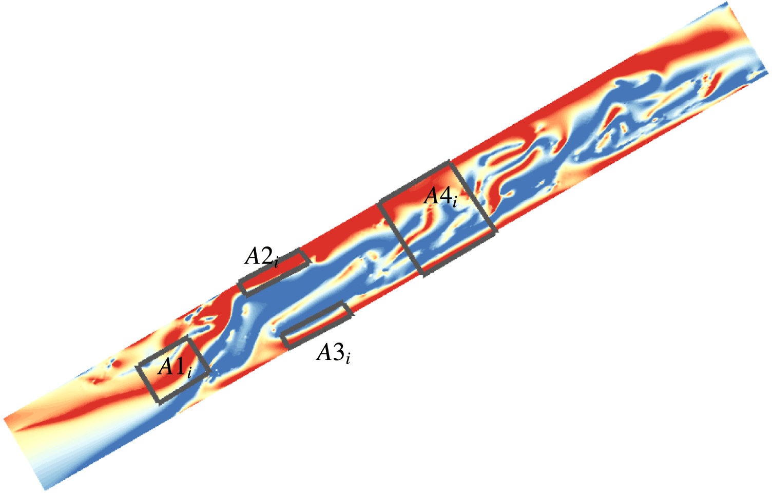
where $A$ is a measurement window inside the 2-D channel and $\unicode[STIX]{x1D714}_{z}$ is the vorticity component in the $z$ direction. Four measurement windows are used in the current study, see figure 11. First, the channel domain is divided into $20$ equal subsections along the axis. Within each subsection, we have $i/2\leqslant x\leqslant (i+1)/2$ , with $i=0:19$ . Then $A1_{i}$ denotes the region in the middle of the channel for various subsections along the axis, with the integration taking place over $-0.3\leqslant y\leqslant 0.3$ . Similarly, $A2_{i}$ and $A3_{i}$ denote the regions close to the top and bottom wall, respectively, corresponding to integration over $0.4\leqslant y\leqslant 0.5$ and $-0.5\leqslant y\leqslant -0.4$ for various subsections. Finally, $A4_{i}$ denotes the region across the entire channel subsection, with integration over $-0.5\leqslant y\leqslant 0.5$ . Here $x,y$ are the non-dimensional coordinates along and perpendicular to the channel axis.

Figure 11.

Sketch of four typical measurement windows $A1_{i}$ – $A4_{i}$ along the channel axis over which the vorticity balance is computed. $A1_{i}$ – $A4_{i}$ with $i=0:19$ are within $20$ equal subsections along the axis.

Figure 12.

Temporal evolution of circulations at different windows along the channel axis. (a) $A1$ , (b) $A2$ , (c) $A3$ and (d) $A4$ . The heavy fluid is placed at the top of the inlet.

Figure 13.

Time history of circulation at different windows along the channel axis: 1, 2, 4, 7. The heavy fluid is placed at the top of the inlet.

Figure 14.

Temporal evolution of circulation within various measurement windows along the channel axis. (a) $A1$ , (b) $A2$ , (c) $A3$ and (d) $A4$ . The heavy fluid is placed at the bottom of the inlet.

Figure 12 shows the temporal evolution of circulation within various measurement windows along the channel axis for the case with the heavy fluid placed as the top layer in the inlet. If we isolate a slice at any axial position, we can observe the change of circulation with time by the variation of the colour. Figure 13 shows the time history of circulations at different windows along the channel axis: $1,2,4,7$ .

We find that $x=2$ is a critical position, as it corresponds to the stagnation point of the back flow on the bottom wall. Specifically, the net circulation around $A4$ is positive in subsection $x<2$ ; we find that the amount of positive circulation produced by the unstable oscillating jet flow in figure 7 is higher than that of negative circulation generated from the top and bottom wall surfaces. However, in the subsection $x\geqslant 2$ , the circulation fluctuates as the vortex shedding becomes erratic along the channel axis. In the top wall region $A2$ , a positive circulation is observed at $x\geqslant 2$ , occasionally increasing in intensity due to the interaction of vorticity shed from the jet. In the middle region $A1$ , a negative circulation is seen at $x\geqslant 2$ , a combination of vorticity generated from the messy shedding of the jet and the rolling waves of back flow. Furthermore, on the bottom wall region $A3$ , the back flow continuously induces positive circulation.

Similarly, we analyse the circulation dynamics when the heavy fluid is injected as the bottom layer in the inlet; see figure 14. The heavy liquid slug reaches a quasi-steady state after $t=45~\text{s}$ . Specifically, at $x\leqslant 2$ , the circulation is negative in the middle region ( $A1$ ), corresponding to the initially formed heavy fluid slug and the generation of negative vorticity from its top interface. Meanwhile, the circulation at $x\leqslant 2$ near the top wall region ( $A2$ ) is almost equal to that in the middle region ( $A1$ ). On the bottom wall region ( $A3$ ), the circulation is almost zero at $x\leqslant 2$ due to the cross-annihilation of opposite-sign vorticity generated between the right surface of the slug and the bottom wall of channel. At the subsections with $2\leqslant x\leqslant 3$ , the circulation ( $\unicode[STIX]{x1D6E4}_{1}$ ) starts oscillating as function of time, corresponding to the unstable vortex shedding in figure figure 10. At the subsections with $4\leqslant x\leqslant 6$ , intermittent behaviour is seen for the circulation in both the ( $A1$ ) and ( $A2$ ) regions, which corresponds to the irregular crushing of the heavy liquid slug on the right surface and its interaction with the vortex shedding from the top wall. However, at the subsections with $6\leqslant x\leqslant 8.5$ , the circulation fluctuates randomly in the region ( $A1$ ), due to contribution of negative circulation from the unsteady rolling waves. Nevertheless, near the bottom wall region ( $A3$ ), positive circulation is found due to vorticity generation from the back flow along the bottom wall.

In summary, in both cases, the net circulation on the entire channel section ( $A4$ ) shows that the vorticity generated from the two-phase flow interfaces and the channel walls is generally negative, while positive vorticity is contributed by the oscillating jet and the back flow inside the inclined pipe.

3.4 Comparison against the horizontal channel

In this subsection we study the effect of the inclination angle on the two-phase flow mechanisms inside the channel when the heavy fluid is the top layer. In figure 15, we have found that, due to the gravity effect, the injected heavy fluid accumulates on the bottom wall of the horizontal channel. As the flow develops, the heavy fluid layer moves to the exit of the channel smoothly. For the inclined channel, we no more observe the back flow or the rolling waves, as shown in figure 7.

Figure 15.

Instantaneous two-phase flow pattern in a 2-D horizontal channel. At the inlet, the heavy liquid is placed as the top layer. Blue colour stands for the heavy fluid while red stands for the light liquid.

As shown in § 2.4, a stratified flow is induced in the horizontal channel. We show here that when the heavy fluid is placed as the top layer, an unsteady flow transition is obtained in the upstream part of the channel, while a stratified wavy flow can still be found in the downstream part of the channel.