





1. Introduction
Stratified flows are common in geophysical systems such as the atmosphere or the oceans (Gill Reference Gill1982). The variation of fluid density along the direction of gravity results in forces that can be either stabilizing or destabilizing. Unstable stratification occurs when denser fluid is atop lighter fluid, which enhances vertical mixing through the formation of large convection cells (e.g. Brown Reference Brown1980; Pirozzoli et al. Reference Pirozzoli, Bernardini, Verzicco and Orlandi2017). This configuration is typically encountered in the atmospheric boundary layer at daytime, when the warm ground heats the surrounding air (e.g. Kaimal et al. Reference Kaimal, Wyngaard, Haugen, Coté, Izumi, Caughey and Readings1976). On the other hand, lighter fluid atop of heavier fluid results in stable stratification, which suppresses vertical motions and gives rise to internal gravity waves (e.g. Mowbray & Rarity Reference Mowbray and Rarity1967). This configuration is typical of the nocturnal atmospheric boundary layer (e.g. Nieuwstadt Reference Nieuwstadt1984), and in the oceans which are heated from above (Wunsch & Ferrari Reference Wunsch and Ferrari2004). These flows often also involve shear and, as such, the interplay of buoyancy and shear is key to the dynamics of geophysical flows through, e.g. mixing (Caulfield Reference Caulfield2021), energetics (Winters et al. Reference Winters, Lombard, Riley and Dásaro1995) and sediment transport (Hung, Niu & Chou Reference Hung, Niu and Chou2020). The present work examines stably stratified wall-bounded shear flows, in the canonical setting of turbulence in a rectilinear channel. We study the linear and nonlinear effects that lead to localization of internal gravity waves in the channel core, using data from direct numerical simulations (DNS).
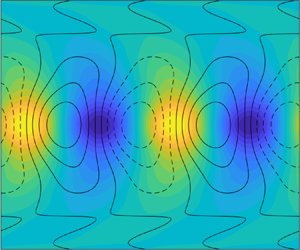
The stratification level of a channel flow is set globally through the density, or equivalently the temperature, difference between the two walls. For our analysis, we consider two stably stratified flows with temperature as the stratifying agent. The relative importance of shear and buoyancy changes with wall-normal height, which leads to local flow regions with distinct characteristics (Armenio & Sarkar Reference Armenio and Sarkar2002; García-Villalba & del Álamo Reference García-Villalba and del Álamo2011). For the present study, the stratified flow is conceptually divided into three layers, which are contrasted with the unstratified configuration in figure 1. The inner region, which is located next to the wall and illustrated by the grey vortical structures, is shear dominated and remains largely unaffected by buoyancy, except for the damped influence of the large-scale motions (García-Villalba & del Álamo Reference García-Villalba and del Álamo2011). The adjacent outer region is represented by the vortical structures coloured by wall distance and will be shown to be essential for the sustenance and localization of the gravity waves. The core region, which is located in the channel centre and delineated by the two horizontal lines, is characterized by low shear and strong gravity effects, which give rise to large-scale internal waves (Armenio & Sarkar Reference Armenio and Sarkar2002; Iida, Kasagi & Nagano Reference Iida, Kasagi and Nagano2002; García-Villalba & del Álamo Reference García-Villalba and del Álamo2011; Lloyd, Dorrell & Caulfield Reference Lloyd, Dorrell and Caulfield2022). These waves are constrained in their wall-normal extent, and carry large flow perturbations, as illustrated by the temperature fluctuations plotted at multiple cross-sections in figure 1.
Unstratified (a) and temperature stratified channel flow (b). The cross-flow planes show the temperature fluctuations and the side panel shows the mean temperature (colour contours) and fluctuations (line contours). The isosurfaces visualize vortical structures. The stratified flow can conceptually be divided into an inner (grey isosurfaces), outer (isosurfaces coloured by distance from the wall) and core region (between the horizontal lines).

These gravity-wave disturbances exhibit linear characteristics in two respects: firstly, the dominant vertical velocity and density (temperature) fluctuations in the channel centre are spatially shifted relative to one another by a quarter wavelength ( ${\rm \pi} /2$ phase shift in Fourier domain), in agreement with linear theory. This phase locking decreases the ensemble-averaged buoyancy flux and steepens the density gradient in the channel centre (see colour contours on the side panel in figure 1 and the discussion by Armenio & Sarkar Reference Armenio and Sarkar2002; García-Villalba & del Álamo Reference García-Villalba and del Álamo2011). Secondly, these gravity-wave disturbances approximately follow a generalized version of the linear dispersion relationship, which properly accounts for the streamwise mean flow and wall-normal extent of the waves. At each streamwise length scale, there is evidence for two wave-like solutions consisting of a dominant upstream travelling and a weaker downstream travelling wave, relative to the frame of the mean flow (Moestam & Davidson Reference Moestam and Davidson2005; Lloyd et al. Reference Lloyd, Dorrell and Caulfield2022).
The observations by Lloyd et al. (Reference Lloyd, Dorrell and Caulfield2022) suggest that the internal waves are generated when hairpin-like disturbances originating from the outer flow region interact with the strong density gradient in the channel core. Linear dynamics seem to play a key role in this process as well. The same authors show that simplified linearized flow models, namely solutions to the two-dimensional (2-D) viscous Taylor–Goldstein equations and the stochastically forced 2-D linearized Navier–Stokes equations (NSE), qualitatively reproduce the flow structure in the core region and the low-frequency branch of the dispersion relation. The linearized system is most sensitive to stochastic forcing in the outer region, which supports the view that the shear-driven turbulence in the near-wall and outer regions sustains the gravity waves in the channel centre. The conclusions from these simplified systems are informative, and we herein aim to complement them with a quantitative assessment of the linear and nonlinear contributions to gravity waves in a three-dimensional flow.
Evidence for the importance of linear mechanisms in shear flows is well established (Phillips Reference Phillips1969), and recent techniques have facilitated their study (see e.g. Jovanović (Reference Jovanović2021) for an overview). One commonly adopted approach is to view the NSE as an input–output system, in which the linearized dynamics, which are represented by the resolvent operator, map a forcing (system input) to an observable flow response (output). The appropriate choice of linearization point, forcing and observable depends on the application. For stationary turbulent flows, the reference state is usually the mean flow, the observable is taken to be the flow state and the forcing is given by the nonlinear advection terms, so that the input–output system is closed (McKeon & Sharma Reference McKeon and Sharma2010). Analysis of unstratified wall-bounded turbulent flows shows that the resolvent is low rank at energetic length scales (Moarref et al. Reference Moarref, Sharma, Tropp and McKeon2013), selectively generates structures that resemble coherent flow motions observed in experiments and numerical simulations (Sharma & McKeon Reference Sharma and McKeon2013), and qualitatively captures the flow response to control and other external inputs (e.g. Luhar, Sharma & McKeon Reference Luhar, Sharma and McKeon2014b; Toedtli, Luhar & McKeon Reference Toedtli, Luhar and McKeon2019). Recently, the resolvent framework has been extended to turbulent flows with stable and unstable stratification (Ahmed et al. Reference Ahmed, Bae, Thompson and McKeon2021; Madhusudanan et al. Reference Madhusudanan, Illingworth, Marusic and Chung2022; Cossu Reference Cossu2023). The linearly most amplified structures change under weak stable stratification in accordance with DNS results. In particular, the linearly most amplified velocity and temperature responses in the near-wall region are inappreciably affected by stratification, but change significantly in the outer flow (Ahmed et al. Reference Ahmed, Bae, Thompson and McKeon2021). Nonetheless, the importance of the linear dynamics, represented by the resolvent operator, for the internal gravity waves remains unexplored and it is not clear, for example, if the resolvent captures their localization in spectral space and in the wall-normal direction.
The characterization of the nonlinear forcing remains a challenge for all input–output formulations of the NSE. It is well known that the forcing has a scale-dependent structure (‘colour’), which has far-reaching implications for the relative amplitude and phase of the linearly amplified structures (see e.g. Zare, Jovanović & Georgiou Reference Zare, Jovanović and Georgiou2017). Aspects of the nonlinear-forcing structure can be incorporated into the linear operator to improve the linear predictions (Morra et al. Reference Morra, Semeraro, Henningson and Cossu2019; Pickering et al. Reference Pickering, Rigas, Schmidt, Sipp and Colonius2021; Liu, Caulfield & Gayme Reference Liu, Caulfield and Gayme2022; Symon et al. Reference Symon, Madhusudanan, Illingworth and Marusic2023) or can be reverse-engineered from flow statistics (Moarref et al. Reference Moarref, Jovanović, Tropp, Sharma and McKeon2014; Zare et al. Reference Zare, Jovanović and Georgiou2017; Rosenberg & McKeon Reference Rosenberg and McKeon2019; Towne, Lozano-Durán & Yang Reference Towne, Lozano-Durán and Yang2020). The true spectral properties of the nonlinear forcing are described by its cross-spectral density (CSD) tensor, which can be computed directly from highly resolved data (see e.g. Towne, Schmidt & Colonius Reference Towne, Schmidt and Colonius2018). Morra et al. (Reference Morra, Nogueira, Cavalieri and Henningson2021) performed a direct calculation of the forcing CSD from DNS data of an unstratified channel flow and confirmed that the forcing is structured and low rank, but not necessarily aligned with the linearly most amplified disturbances. The effect of stratification on the forcing CSD and the role of nonlinear forcing for the sustenance and localization of internal gravity waves remains unexplored. Another interesting aspect of the nonlinearity is that the flow response to individual forcing components (e.g. in-plane and vertical momentum forcing) can interfere constructively or destructively, depending on the relative phase imprinted by the nonlinearity. Destructive interference is commonly observed in unstratified flows and becomes most apparent in the velocity–vorticity formulation in channel flows (Rosenberg & McKeon Reference Rosenberg and McKeon2019; Morra et al. Reference Morra, Nogueira, Cavalieri and Henningson2021). It is conceivable that destructive interference is also important in stably stratified flows, especially for the localization of internal gravity waves, but this aspect has not been previously explored.
This paper aims to address some of the gaps identified in the literature. Specifically, our study quantifies the contributions of the linear and nonlinear dynamics to the localization of internal gravity waves by analysing DNS data of two stably stratified turbulent channel flows. Section 2 introduces the problem formulation, describes the DNS and outlines the data processing and analysis tools. Time-averaged flow statistics and spatio-temporal CSDs are computed from DNS data for the flow response and for the nonlinear forcing. Section 3 presents these DNS data to illustrate the effect of stratification on the flow response and forcing, and to identify the length and time scales representative of internal gravity waves. The linear dynamics associated with the stratified resolvent operator are analysed in § 4. The analysis is focused on the gravity waves and shows that the spectral localization is determined by the linear dynamics, but information about the nonlinearity is required to understand the wall-normal localization. Section 5 studies the nonlinear-forcing CSD and explores its role in sustaining and localizing the gravity waves. In this context, it is shown that the flow has a three-layer structure (as indicated in figure 1) and that the forcing in the outer region generates the majority of the flow response in the channel core. Velocity and temperature forcing further induce distinct phase relations that lead to destructive interference and localization of the gravity waves in the channel core.
2. Approach
This section introduces the mathematical problem formulation and outlines the data acquisition. The governing equations and their input–output form are summarized in § 2.1. Section 2.2 describes the DNS that generated the data and the post-processing steps to transform the DNS data into a suitable representation for subsequent analysis.
2.1. Governing equations and input–output form
We consider a temperature stratified turbulent channel flow with periodic streamwise ( ${x}^{\star }$) and spanwise (
 ${z}^{\star }$) directions, and walls located at
 ${y}^{\star } = \{ 0, 2{h}^{\star } \}$ (see figure 1). The net mass flux in the streamwise direction is constant, and the no-slip walls (
 ${u}^{\star } = {v}^{\star } = {w}^{\star } = 0$) are maintained at constant but different temperatures. The top wall is
 $\Delta {T}^{\star }$ hotter than the bottom one, which induces a stable stratification in the vertical direction, aligned with the mean shear.
The temperature-induced density fluctuations are assumed to be small relative to the background density, and therefore, the Boussinesq approximation can be invoked. The governing equations are the incompressible NSE combined with a transport equation for the temperature field, which in non-dimensional form are
 \begin{gather} \boldsymbol{\nabla} \boldsymbol{\cdot} \boldsymbol{u} = 0, \end{gather}
 \begin{gather}\partial_{t} \boldsymbol{u} + \boldsymbol{u} \boldsymbol{\cdot} \boldsymbol{\nabla} \boldsymbol{u} ={-} \boldsymbol{\nabla} \tilde{p} + \frac{1}{{Re}_{b}} \nabla^2 \boldsymbol{u} + {Ri}_{b} \, T \boldsymbol{e}_y, \end{gather}
 \begin{gather}\partial_{t} T + \boldsymbol{u} \boldsymbol{\cdot} \boldsymbol{\nabla} T = \frac{1}{{Pr} \, {Re}_{b}} \nabla^2 T . \end{gather}
These equations will collectively be referred to as ‘NSE’ hereafter. In the above expression,  $\boldsymbol {u} = (u, v, w)^{\top }$ is the velocity vector,
 $T$ represents temperature,
 $t$ denotes time,
 $\tilde {p} = p - p_{h}$ is the difference between the kinematic pressure (
 $p$) and the hydrostatic pressure of the constant background density (
 $p_{h}$), and
 $\boldsymbol {e}_y$ is the unit vector in the wall-normal direction. All flow quantities are made dimensionless with the channel half-height (
 ${h}^{\star }$), bulk velocity (
 ${U}^{\star }_b$) and half the temperature difference between the walls (
 $\Delta {T}^{\star } / 2$). The resulting non-dimensional problem parameters are the Prandtl number
 $Pr = {\nu }^{\star } / {\kappa }^{\star }$ (where
 ${\nu }^{\star }$ is the kinematic viscosity and
 ${\kappa }^{\star }$ the thermal diffusivity of the fluid), Reynolds number
 ${Re}$ and Richardson number
 ${Ri}$. The Reynolds and Richardson numbers can be defined with respect to the bulk (
 ${U}^{\star }_b$) or friction (
 ${u}^{\star }_{\tau }$) velocities,
 \begin{gather} {Re}_{b} = \frac{{U}^{{\star}}_b {h}^{{\star}}}{{\nu}^{{\star}}} ,\quad {Ri}_{b} = \frac{{\alpha}^{{\star}} \Delta {T}^{{\star}} {g}^{{\star}} {h}^{{\star}}}{2 {{U}^{{\star}}_b}^2}, \end{gather}
 \begin{gather}{Re}_{\tau} = \frac{{u}^{{\star}}_{\tau} {h}^{{\star}}}{{\nu}^{{\star}}} ,\quad {Ri}_{\tau} = \frac{{\alpha}^{{\star}} \Delta {T}^{{\star}} {g}^{{\star}} {h}^{{\star}}}{{{u}^{{\star}}_{\tau}}^2}, \end{gather}
where  ${g}^{\star }$ denotes the gravitational acceleration and
 ${\alpha }^{\star }$ is the thermal expansion coefficient. The majority of the results will be presented using inner scaling, and where helpful bulk quantities will be reported.
In order to classify dynamical contributions as linear or nonlinear, we rewrite (2.1) in input–output form, which leads to the so-called resolvent formulation of the NSE. Formally, any flow variable  $\zeta$ is Reynolds decomposed into a spatio-temporal mean
 $\overline {\zeta }(y)$ and fluctuations
 ${\zeta }^{\prime }(x, y, z, t)$. With knowledge of the mean-flow profiles, we turn to the fluctuation equations where we group all linear terms on the left-hand side, while the nonlinear terms are isolated on the right-hand side. The fluctuation equations are Fourier transformed in the homogeneous spatial directions (
 $x$ and
 $z$) and in time, using
 \begin{equation} \hat{\zeta}_{\boldsymbol{k}}(y) = {\mathcal{F} \{ \zeta \}} = \frac{1}{2 {\rm \pi} L_{x} L_{z}} \int_{-\infty}^{\infty} \int_0^{L_x} \int_0^{L_z} \zeta(x, y, z, t) \,{\rm e}^{-{\rm i}( k_x x + k_z z - \omega t )} \, \mathrm{d} z \, \mathrm{d}\kern0.06em x \, \mathrm{d} t. \end{equation}
Due to the finite size of the domain in  $x$ (with period
 $L_x$) and
 $z$ (period
 $L_z$), the associated wavenumbers
 $k_x = k (2{\rm \pi} / L_x)$ and
 $k_z = l (2{\rm \pi} / L_z)$ are constrained to integer multiples (
 $\{ k, l \} \in \mathbb {Z}$) of the fundamentals. The wavenumbers are collected in the vector
 $\boldsymbol {k} = (k_x, k_z, \omega )^{\top }$ and a single Fourier mode will be referred to as
 $\hat {\zeta }_{\boldsymbol {k}}$, where the superscript hat indicates a complex-valued quantity. Note that the sign convention in the Fourier transform of the spatial and temporal directions is different, so that a Fourier mode with positive
 $k_x$ and
 $\omega$ advects downstream at wave speed
 $c = \omega / k_x$.
With these manipulations, the fluctuation equations at each  $\boldsymbol {k} \neq \boldsymbol {0}$ can be expressed as
 \begin{equation} - ( {\rm i} \omega \boldsymbol{\mathsf{M}} + \boldsymbol{\mathsf{L}} ) \boldsymbol{\mathsf{D}} \hat{\boldsymbol{q}}_{\boldsymbol{k}} = \boldsymbol{\mathsf{B}} \hat{\tilde{\boldsymbol{f}}}_{\boldsymbol{k}}, \end{equation}
where the state vector  $\hat {\boldsymbol {q}}_{\boldsymbol {k}}$ and the nonlinear-forcing vector
 $\hat {\tilde {\boldsymbol {f}}}_{\boldsymbol {k}}$ are given by
 \begin{equation} \hat{\boldsymbol{q}}_{\boldsymbol{k}} = \begin{pmatrix} \hat{u}_{\boldsymbol{k}} \\ \hat{v}_{\boldsymbol{k}} \\ \hat{w}_{\boldsymbol{k}} \\ \hat{T}_{\boldsymbol{k}} \end{pmatrix}, \quad \hat{\tilde{\boldsymbol{f}}}_{\boldsymbol{k}} = \begin{pmatrix} \widehat{\tilde{f}_{u}}_{\boldsymbol{k}} \\ \widehat{\tilde{f}_{v}}_{\boldsymbol{k}} \\ \widehat{\tilde{f}_{w}}_{\boldsymbol{k}} \\ \widehat{\tilde{f}_{T}}_{\boldsymbol{k}} \end{pmatrix}= \begin{pmatrix} -(\widehat{{\boldsymbol{u}}^{\prime} \boldsymbol{\cdot} \boldsymbol{\nabla} {u}^{\prime}})_{\boldsymbol{k}} \\ -(\widehat{{\boldsymbol{u}}^{\prime} \boldsymbol{\cdot} \boldsymbol{\nabla} {v}^{\prime}})_{\boldsymbol{k}} \\ -(\widehat{{\boldsymbol{u}}^{\prime} \boldsymbol{\cdot} \boldsymbol{\nabla} {w}^{\prime}})_{\boldsymbol{k}} \\ -(\widehat{{\boldsymbol{u}}^{\prime} \boldsymbol{\cdot} \boldsymbol{\nabla} {T}^{\prime}})_{\boldsymbol{k}} \end{pmatrix} = \widehat{\boldsymbol{f}_i}_{\boldsymbol{k}} + \hat{\boldsymbol{f}}_{\boldsymbol{k}}, \end{equation}
and the operators  $\boldsymbol{\mathsf{M}}$,
 $\boldsymbol{\mathsf{L}}$,
 $\boldsymbol{\mathsf{D}}$ and
 $\boldsymbol{\mathsf{B}}$ are defined in Appendix A. The operators themselves depend on the wavenumber vector, but the subscript
 $\boldsymbol {k}$ is omitted for compactness. The nonlinear forcing can further be split into irrotational (
 $\boldsymbol {f}_i)$ and solenoidal (
 $\boldsymbol {f}$) parts. The former lies in the null space of the operator
 $\boldsymbol{\mathsf{B}}$, so that the solenoidal part alone determines the velocity response (see e.g. Chorin & Marsden Reference Chorin and Marsden1993). We will therefore replace
 $\hat {\tilde {\boldsymbol {f}}}_{\boldsymbol {k}}$ in (2.4) by
 $\hat {\boldsymbol {f}}_{\!\boldsymbol {k}}$ and only report the dynamically relevant solenoidal part of the forcing. Note that the temperature forcing is not subject to the solenoidal constraint, and therefore,
 $\widehat {\tilde {f}_T}_{\boldsymbol {k}} = \widehat {f_T}_{\boldsymbol {k}}$.
The operator on the left-hand side of (2.4) can be inverted to obtain the NSE in input–output form. The linear operator that maps the nonlinear forcing  $\hat {\boldsymbol {f}}_{\!\boldsymbol {k}}$ (considered the input) to the flow response
 $\hat {\boldsymbol {q}}_{\boldsymbol {k}}$ (output) is called the resolvent operator
 $\boldsymbol{\mathsf{R}}$,
 \begin{equation} \hat{\boldsymbol{q}}_{\boldsymbol{k}} ={-} \boldsymbol{\mathsf{C}} ({\rm i} \omega \boldsymbol{\mathsf{I}} + \boldsymbol{\mathsf{L}}_1 )^{{-}1} \boldsymbol{\mathsf{B}}_1 \,\hat{\boldsymbol{f}}_{\boldsymbol{k}} = \boldsymbol{\mathsf{R}} \hat{\boldsymbol{f}}_{\boldsymbol{k}}, \end{equation}
where  $\boldsymbol{\mathsf{L}}_1 = \boldsymbol{\mathsf{M}}^{-1} \boldsymbol{\mathsf{L}}$ and
 $\boldsymbol{\mathsf{B}}_{1} = \boldsymbol{\mathsf{M}}^{-1} \boldsymbol{\mathsf{B}}$; the definition of the operator
 $\boldsymbol{\mathsf{C}}$ is given in Appendix A. It is important to point out that the resolvent depends on the choice of input and output variables. Other definitions would be possible, for example, if the NSE were formulated in velocity–vorticity form. It should also be noted that (2.6) is an exact representation of the NSE at each
 $\boldsymbol {k}$ when the mean-velocity and mean-temperature profiles are known.
The resolvent formulation provides a natural partitioning of the flow dynamics and stratification effects into linear and nonlinear interpretations, as illustrated by the block diagram of figure 2. Past studies typically analyse one of the two blocks (see e.g. Morra et al. Reference Morra, Nogueira, Cavalieri and Henningson2021; Huang et al. Reference Huang, Toedtli, Chini and McKeon2023), and following this approach we focus on the lower half of the diagram. Starting from the flow response  $\boldsymbol {q}_{\boldsymbol {k}}$, the present study investigates how the resolvent
 $\boldsymbol{\mathsf{R}}$ and nonlinear forcing
 $\boldsymbol {f}_{\boldsymbol {k}}$ localize internal gravity waves in spectral space and in the channel core. We will term flow features associated with the resolvent operator
 $\boldsymbol{\mathsf{R}}$ as linear effects, which will be studied in § 4. Phenomena associated with the forcing
 $\hat {\boldsymbol {f}}_{\!\boldsymbol {k}}$ will be classified as nonlinear effects, and are the subject of § 5.
(a) Block diagram of the NSE in resolvent form. (b,c) Components of the CSD tensor for the flow response ( $\hat {\boldsymbol{\mathsf{S}}}_{\boldsymbol {k}}$) and forcing (
 $\hat {\boldsymbol{\mathsf{P}}}_{\boldsymbol {k}}$). (d,e) Physical flow structure of the leading forcing SPOD mode (
 $\hat {\boldsymbol {\chi }}_1$) and associated flow response (
 $\boldsymbol{\mathsf{R}} \hat {\boldsymbol {\chi }}_1$).

2.2. Data acquisition and processing
The input–output framework is applied to high-fidelity data obtained from DNS of a turbulent channel flow at  ${Re}_{\tau } \approx 180$. Three conditions are considered: an unstratified case (
 ${Ri}_{\tau } = 0$, labelled ‘R0’), which serves as a reference, and two stratified ones. The weakly stratified simulation at
 ${Ri}_{\tau } \approx 60$ (labelled ‘R60’) will be the main focus of this study, and the last computation at
 ${Ri}_{\tau } \approx 120$ (labelled ‘R120’) is analysed to verify that the results generalize to more strongly stratified flows. For a given
 ${Re}_{\tau }$, the feasible range of Richardson numbers is limited by the requirement that the majority of the flow stay fully turbulent, so that the Reynolds decomposition remains physically meaningful. The simulations discussed herein cover the feasible
 ${Ri}$ range at
 ${Re}_{\tau } \approx 180$, in accordance with earlier results by García-Villalba & del Álamo (Reference García-Villalba and del Álamo2011). The relevant flow parameters of all cases are summarized in table 1. The Nusselt number is defined as
 $Nu = {d}_{y} \overline {{T}^{\star }}|_{{y}^{\star } = 0} (2 {h}^{\star } / \Delta {T}^{\star })$ and the expressions for the other non-dimensional groups can be found in (2.2).
Flow parameters for unstratified (R0) and stratified flows (R60, R120).

2.2.1. Direct numerical simulation
The DNS uses a fractional step method with local volume fluxes in a staggered grid arrangement, as described in Rosenfeld, Kwak & Vinokur (Reference Rosenfeld, Kwak and Vinokur1991). The time-stepping algorithm is Adams–Bashforth for the nonlinear advection terms and Crank–Nicolson for the diffusive terms. The pressure Poisson equation is solved with Fourier transforms in the periodic streamwise and spanwise directions, leading to a tridiagonal system that can be solved efficiently. The code has been extensively validated in unstratified transitional (Marxen & Zaki Reference Marxen and Zaki2019; Wang, Wang & Zaki Reference Wang, Wang and Zaki2019a) and fully turbulent channel flows (Wang, Hasegawa & Zaki Reference Wang, Hasegawa and Zaki2019b; Wang & Zaki Reference Wang and Zaki2021), and further validation for the stratified case is presented in §§ 3 and 5.
The channel flow is driven by a constant mass flux and the bulk Reynolds number is increased with stratification, so that  ${Re}_{\tau } \approx 180$ in all cases. The domain size and grid resolution are summarized in table 2. The superscript plus indicates normalization with respect to the viscous scales (
 ${u}^{\star }_{\tau }$ and
 ${\nu }^{\star } / {u}^{\star }_{\tau }$), which are approximately constant across flow configurations. The grid is uniform in the streamwise and spanwise directions, and the non-uniform grid spacing in
 $y$ follows a stretched hyperbolic tangent function. A larger domain size is required to sustain turbulence in configuration R120, and the
 $\{x, z\}$ grid resolutions are reduced to keep the storage requirements feasible. The grid is only slightly coarser compared to previous DNS studies (e.g. García-Villalba & del Álamo Reference García-Villalba and del Álamo2011; Ahmed et al. Reference Ahmed, Bae, Thompson and McKeon2021); even so our analysis will put less emphasis on this coarser simulation. The time step is fixed ({R0, R60}:
 $\Delta t^+ = 0.045$, R120:
 $\Delta t^+ = 0.034$) and the total integration times are
 ${t}^{\star } ({u}^{\star }_{\tau } / {h}^{\star }) = \{ 210, 204, 187 \}$ for {R0, R60, R120}, respectively. A total of
 $10\,001$ flow snaspshots
 $\boldsymbol {q}(x, y, z, t)$ are collected for each configuration at a constant sampling interval of
 $\Delta t_s^{+} \approx \{ 3.7, 3.6, 3.4\}$, resulting in
 $16$ TB of data per flow condition.
Domain size and grid parameters. The variables  $N_x$,
 $N_y$ and
 $N_z$ denote the number of grid points in each direction. Note that the horizontal domain size and grid resolution are different for case R120.

2.2.2. Data processing
The input–output relation in (2.6) is defined in Fourier space, while the DNS data are available in physical space on a staggered grid and at constant time intervals. To unify the two perspectives, a spectral representation of the DNS data is obtained in post-processing.
In a first step, the instantaneous DNS fields  $\boldsymbol {q}(x,y,z,t)$ are Fourier transformed in
 $x$ and
 $z$, and spectrally upsampled to
 $(3/2) N_x$ and
 $(3/2) N_z$ wavenumbers. A complex phase shift is then applied to collocate all flow variables on the
 $x$ and
 $z$ vertices of the original spatial grid. The DNS data are subsequently interpolated from the stretched hyperbolic tangent grid in
 $y$ onto Chebyshev collocation points using cubic splines, with an additional zero slope constraint for
 $v$ at
 $y = \{ 0, 2\}$ to enforce continuity at the wall. The appropriate number of Chebyshev collocation points
 $N_c = 161$ is determined as the minimum
 $N$ at which the reconstruction error no longer decreases with an increasing number of collocation points. The collocated velocity fields are divergence free with respect to the finite volume numerics of the DNS, but not necessarily with respect to the spectral operators. We therefore apply a spectral Leray projector
 $\mathbb {P}$ to enforce incompressibility with respect to the Fourier and Chebyshev operators
 \begin{equation} \mathbb{P}(\hat{\boldsymbol{u}}_{\boldsymbol{\xi}} (y, t)) = \hat{\boldsymbol{u}}_{\boldsymbol{\xi}}(y, t) - \boldsymbol{\nabla} \Delta^{{-}1} (\boldsymbol{\nabla} \boldsymbol{\cdot} \hat{\boldsymbol{u}}_{\boldsymbol{\xi}}(y, t)), \end{equation}
where  $\boldsymbol {\xi } = (k_x, k_z)^{\top }$ is the spatial wavenumber vector and
 $\hat {\boldsymbol {u}}_{\boldsymbol {\xi }}$ denotes the
 $\{ x,z \}$ Fourier coefficients of the velocity field. We have further validated that the original and projected velocity fields have the same flow statistics.
The nonlinear terms  $\tilde {\boldsymbol {f}}(x, y, z, t)$, which represent the input in (2.6), are evaluated pseudo-spectrally from the divergence-free part of the collocated flow snapshots. The quadratic advection terms are evaluated in physical space and the
 $(3/2)$ rule is used to dealias the time-dependent spatial Fourier coefficients
 $\hat {\tilde {\boldsymbol {f}}}_{\boldsymbol {\xi }}(y,t)$. Recall that only the divergence-free part of the velocity forcing,
 $\tilde {\boldsymbol {f}}_{\!\boldsymbol {u}}$, is required for the input–output formulation in (2.6), which can be extracted with a similar Leray projector as (2.7),
 \begin{equation} \widehat{\boldsymbol{f}_{\boldsymbol{u}}}_{\boldsymbol{\xi}}(y,t) = \mathbb{P}(\,\widehat{\tilde{\boldsymbol{f}}_{\boldsymbol{u}}}_{\boldsymbol{\xi}}(y, t)). \end{equation}
The final processing step is to estimate the temporal frequency content at each  $\boldsymbol {k}$ of the DNS data. To obtain converged estimates, we average over multiple realizations (Welch's method; see e.g. Towne et al. Reference Towne, Schmidt and Colonius2018), which is achieved by splitting the time series into shorter segments of
 $300$ samples (or time window
 $T_{\eta }$), with 50 % overlap between adjacent blocks; we then apply a Hann window
 $\eta (t)$ to each segment to enforce periodicity:
 \begin{equation} \eta(t) = \frac{\tilde{\eta}(t)}{\displaystyle\left( \dfrac{1}{T_{\eta}} \int_0^{T_{\eta}} \tilde{\eta}^2(t) \, \mathrm{d}t \right)^{1/2}}, \quad \tilde{\eta}(t) = \sin^2\left( \frac{{\rm \pi} t}{T_{\eta}} \right) \text{ for } 0 \leq t \leq T_{\eta}. \end{equation}
It is important to point out that the window function introduces additional temporal dynamics, since  $\eta (t)$ does not commute with the time derivative. The window dynamics have to be accounted for in (2.6) by replacing
 $\hat {\boldsymbol {q}}_{\boldsymbol {k}}$ and
 $\hat {\boldsymbol {f}}_{\!\boldsymbol {k}}$ by
 \begin{equation} \hat{\boldsymbol{q}}_{\eta \boldsymbol{k}} = \begin{pmatrix} \widehat{(u \eta)}_{\boldsymbol{k}} \\ \widehat{(v \eta)}_{\boldsymbol{k}} \\ \widehat{(w \eta)}_{\boldsymbol{k}} \\ \widehat{(T \eta)}_{\boldsymbol{k}} \end{pmatrix},\quad \hat{\boldsymbol{f}}_{\eta \boldsymbol{k}} = \begin{pmatrix} \widehat{(f_u \eta)}_{\boldsymbol{k}} + \widehat{(u {d}_{t} \eta)}_{\boldsymbol{k}} \\ \widehat{(f_v \eta)}_{\boldsymbol{k}} + \widehat{(v {d}_{t} \eta)}_{\boldsymbol{k}} \\ \widehat{(f_w \eta)}_{\boldsymbol{k}} + \widehat{(w {d}_{t} \eta)}_{\boldsymbol{k}} \\ \widehat{(f_T \eta)}_{\boldsymbol{k}} + \widehat{(T {d}_{t} \eta)}_{\boldsymbol{k}} + {d}_{y} (\overline{vT}) \hat{\eta}(\omega) \delta_{k_{x}0} \, \delta_{k_{z}0} \end{pmatrix}, \end{equation}
where  $\delta _{k_x 0}$ is the Kroenecker Delta in the Fourier domain. This is an inherent limitation of analysing the temporal frequency content of non-periodic signals. All reported temporal statistics of the nonlinear-forcing terms contain the additional window dynamics, since this is required to satisfy the input–output relation equation (2.6) to satisfactory accuracy (see also Morra et al. (Reference Morra, Nogueira, Cavalieri and Henningson2021) for additional details).
2.2.3. Spectral densities
Spectral densities are used to statistically characterize the turbulence and the forcing, at individual length and time scales. The CSD tensor is an appropriate statistical characterization of the Fourier coefficients, which we compute following the algorithm by Towne et al. (Reference Towne, Schmidt and Colonius2018). The CSD of the turbulence is denoted as  $\hat {\boldsymbol{\mathsf{S}}}_{\boldsymbol {k}}$ and that of the forcing is denoted as
 $\hat {\boldsymbol{\mathsf{P}}}_{\boldsymbol {k}}$. Both quantities are formally defined as
 \begin{gather} \hat{\boldsymbol{\mathsf{S}}}_{\boldsymbol{k}}(y, y^{\prime}) = \mathbb{E} [ \hat{\boldsymbol{q}}_{\eta \boldsymbol{k}}(y) \hat{\boldsymbol{q}}_{\eta \boldsymbol{k}}^H (y^{\prime}) ], \end{gather}
 \begin{gather}\hat{\boldsymbol{\mathsf{P}}}_{\boldsymbol{k}}(y, y^{\prime}) = \mathbb{E} [\, \hat{\boldsymbol{f}}_{\eta \boldsymbol{k}}(y) \hat{\boldsymbol{f}}_{\eta \boldsymbol{k}}^H(y^{\prime}) ], \end{gather}
and are shown schematically on the top right of figure 2. Note that each sub-block of  $\hat {\boldsymbol{\mathsf{S}}}_{\boldsymbol {k}}$ and
 $\hat {\boldsymbol{\mathsf{P}}}_{\boldsymbol {k}}$ corresponds to the covariance between different components of the state and forcing vector, respectively. All CSDs are ensemble averaged over the windowed realizations of duration
 $T_{\eta }$ and normalized by the wavenumber (
 $\Delta k_i$) and frequency (
 $\Delta \omega$) spacing to obtain true spectral densities. Equation (2.6) implies that the resolvent relates the CSD of the forcing and the flow response,
 \begin{equation} \hat{\boldsymbol{\mathsf{S}}}_{\boldsymbol{k}} = \mathbb{E} [ \hat{\boldsymbol{q}}_{\eta \boldsymbol{k}} \hat{\boldsymbol{q}}_{\eta \boldsymbol{k}}^H ] = \boldsymbol{\mathsf{R}} \mathbb{E} [\,\hat{\boldsymbol{f}}_{\eta \boldsymbol{k}} \hat{\boldsymbol{f}}_{\eta \boldsymbol{k}}^H ] \boldsymbol{\mathsf{R}}^H = \boldsymbol{\mathsf{R}} \hat{\boldsymbol{\mathsf{P}}}_{\boldsymbol{k}} \boldsymbol{\mathsf{R}}^H. \end{equation}
This input–output relation can be used to verify the convergence and accuracy of the right-hand side in comparison to direct computation of the left-hand side; (2.12) further provides a framework to analyse the flow response generated due to subsets of the forcing  $\hat {\boldsymbol{\mathsf{P}}}_{\boldsymbol {k}}$. Both aspects will be explored in § 5.
The real-valued diagonal terms of the CSD tensors are of particular interest and will be used to illustrate the flow structure at specific  $\boldsymbol {k}$. The diagonal terms are referred to as power spectral densities (PSDs) and are denoted by a corresponding lower-case symbol, with the component indicated in the subscript (for example,
 $\boldsymbol {s}_{\boldsymbol {k} vv}$ and
 $\boldsymbol {p}_{\boldsymbol {k} vv}$). The integral of the PSD over
 $\omega$ recovers the time-averaged PSD (denoted by
 $\boldsymbol {s}_{\boldsymbol {\xi } vv}$,
 $\boldsymbol {p}_{\boldsymbol {\xi } vv}$, etc.) and the integral over
 $\boldsymbol {k}$ is equal to the variance.
3. Flow statistics and spectra
We begin the discussion with the analysis of statistics computed from the DNS of the unstratified and stratified flows. Mean and root-mean-square (r.m.s.) profiles are first discussed in § 3.1 to provide a general view of how the flow changes under stratification and to compare to the literature for validation. Spatial and spatio-temporal PSDs are presented next in §§ 3.2 and 3.3, respectively. They illustrate how stratification changes the energy content in spectral space and guide the selection of a relevant wavenumber triplet  $\boldsymbol {k}$ for subsequent analysis.
3.1. Mean profiles
Select ensemble-averaged statistics are presented in figure 3. The solid lines correspond to the present DNS, with stronger stratification represented by darker lines, while the open symbols are data from the simulations by Ahmed et al. (Reference Ahmed, Bae, Thompson and McKeon2021). The profiles are either anti-symmetric (mean temperature  $\overline {T}$) or symmetric (remaining quantities) about the channel centreline, and only the data in the lower channel half
 $y \in [0, 1]$ are reported. All quantities show good agreement with the data by Ahmed et al. (Reference Ahmed, Bae, Thompson and McKeon2021), which confirms the accuracy of our simulations.
Spatio-temporal mean profiles for different flow configurations. Case R0 (unstratified), light blue; case R60, medium blue; and case R120, dark blue. Lines represent the current simulations, while symbols outline data of Ahmed et al. (Reference Ahmed, Bae, Thompson and McKeon2021). (a) Mean streamwise velocity, (b) mean temperature, (c) r.m.s. of wall-normal velocity, (d) r.m.s. of solenoidal wall-normal velocity forcing, (e) r.m.s. of temperature, (f) r.m.s. of temperature forcing.

The modifications of the mean and r.m.s. velocity and temperature profiles (figure 3a–c,e) due to gravity effects have been extensively discussed by García-Villalba & del Álamo (Reference García-Villalba and del Álamo2011) and we only summarize a few key observations. The near-wall turbulence is little affected by stable stratification and the profiles collapse in this region when normalized by viscous scales. The largest modifications are observed close to the channel centre, where the mean-velocity profile approaches a parabola and the mean-temperature gradient steepens with increasing  ${Ri}$. The wall-normal velocity fluctuations decrease with stratification in the region
 $0.5 < y < 0.9$ and recover the unstratified level only close to the channel centre. In contrast, stratification increases the temperature fluctuations beyond the near-wall region. The largest fluctuations are recorded in the channel centre for R60, and reduce slightly for stronger stratification. It is important to remark that the temperature fluctuations are normalized by the friction temperature
 ${T}^{\star }_{\tau } = ({\kappa }^{\star } / {u}^{\star }_{\tau }) \, {d}_{y} \overline {{T}^{\star }}|_{{y}^{\star }= 0}$, which decreases with stratification (compare the Nusselt numbers in table 1) and, thus, magnifies the r.m.s. profile at higher
 ${Ri}$. Independent of normalization, large
 $v$ and
 $T$ fluctuations are observed in the stratified flow close to the channel centreline, and are typically attributed to the internal gravity waves that occur in this region (García-Villalba & del Álamo Reference García-Villalba and del Álamo2011).
Figure 3(d,f) shows statistics of the nonlinear terms (forcing in the terminology of the input–output framework) of the momentum and temperature equations. As noted in § 2.1, only the dynamically relevant solenoidal part of the momentum forcing is shown. The r.m.s. fluctuations of the  $v$ forcing (figure 3d) increase with
 ${Ri}$ except very near the channel centre, in contrast with the observed decrease in
 $v_{rms}$. As for the r.m.s. temperature forcing (figure 3f), it appreciably exceeds the unstratified curve beyond the near-wall region, even at values of
 $y$ where
 $T_{rms}$ is inappreciably modified. It is important, however, to keep in mind that the comment regarding the normalization by
 ${T}^{\star }_{{\tau }}$ is relevant here as well.
The ensemble-averaged statistics illustrate that stratification acts non-uniformly across the channel. A primary reason is that the strength of gravity effects relative to shear depends on the distance from the wall, leading to flow regions with distinct dynamics and flow characteristics. The relative strength of gravity and shear can be quantified by the gradient Richardson number,
 \begin{equation} {Ri}_g = \frac{{{N}^{{\star}}}^2}{({d}_{y} {\overline{u}}^{{\star}})^2} = \frac{{g}^{{\star}} {\alpha}^{{\star}} {d}_{y} {\overline{T}}^{{\star}}}{({d}_{y} {\overline{u}}^{{\star}})^2} = \left( \frac{{T}^{{\star}}_S}{{T}^{{\star}}_B} \right)^2, \end{equation}
which is a ratio between the time scales of local shear ( ${T}^{\star }_{S}$) and buoyancy (
 ${T}^{\star }_{B}$). The latter is defined in terms of the buoyancy frequency
 ${{N}^{\star }}^2 = {g}^{\star } {\alpha }^{\star } {d}_{y} {\overline {T}}^{\star }$. The gradient Richardson numbers in our stratified simulations are shown in figure 4. In both cases,
 ${Ri}_g$ is small in proximity of the wall, which means that shear dominates over buoyancy. This implies that the near-wall flow is inappreciably affected by stratification, consistent with the agreement of the mean profiles from the stratified and unstratified flows over that region in figure 3. At higher
 $y$, the gradient Richardson number monotonically increases and ultimately diverges since the mean shear vanishes at the channel centreline, and gravity effects become dominant in this region. For our subsequent analysis, we divide the channel into three qualitative regions, which are indicated by different shadings in figure 4: inner region (represented in grey), outer region (no shading) and core region (green shading). The extent of the inner region will be discussed subsequently, while the boundary between the outer and core region is taken at
 $y = 0.8$, in accordance with Lloyd et al. (Reference Lloyd, Dorrell and Caulfield2022).
Gradient Richardson number of the stratified flows. The shaded areas indicate the different conceptual layers in the lower half of the channel. Grey, inner region; white, outer region; green, core region.

3.2. Time-averaged PSDs
The mean profiles of the previous section provide a global sense of flow modification by stratification. In contrast, the input–output view of the NSE (figure 2) is formulated for individual wavenumber triplets and a suitable  $\boldsymbol {k}$ has to be chosen to proceed with the analysis. The choice of
 $\boldsymbol {k}$ is guided by the spectra of the flow response, which delineate the stratification effect at each scale, and with a focus on the channel core where stratification effects are strongest. We will emphasize the wall-normal velocity and temperature in our discussion: these variables are directly coupled by stratification (see (2.1)), admit wave-like solutions to the linearized temperature equation and most clearly show the imprint of internal gravity waves in fully turbulent flows. We first consider time-averaged PSDs, which will inform the selection of the streamwise (
 $k_{x}$) and spanwise wavenumber (
 $k_{z}$). Section 3.3 will present temporal PSDs to guide the choice of
 $\omega$. For conciseness, the discussion focuses on cases R0 and R60; a summary of the relevant spectra for R120 will be given in § 5.4.
Figure 5 shows the time-averaged PSD of  $v$ and
 $T$ (figure 5a,c), as well as their forcing terms (figure 5b,d). The spectra are integrated over
 $k_x$ and recover the square of the fluctuations in figure 3 when integrated over the spanwise wavenumbers. Note that only a subset of the resolved
 $k_{z}$ is shown for clarity. Each spectrum is normalized by its maximum value (indicated above the figure) and the same contour levels
 $\boldsymbol {s}_{\boldsymbol {\xi }} / \max \boldsymbol {s}_{\boldsymbol {\xi }} = \{ 0.25, 0.5, 0.75 \}$ are shown for case R0 (light blue) and R60 (colour contours). We first discuss how the response and forcing PSDs change with stratification, and then contrast the spectral content of the input and output variables.
Time-averaged PSDs as a function of the wall-normal coordinate  $y$ and spanwise wavenumber
 $k_z$. The spectra are integrated over the streamwise wavenumber
 $k_x$ and normalized by their respective maximum value, which is reported above each figure in order {R0 (light blue), R60 (medium blue)}. The contour lines label
 $\boldsymbol {s}_{\boldsymbol {\xi }} / (\max \boldsymbol {s}_{\boldsymbol {\xi }}) = \{ 0.25, 0.5, 0.75 \}$ and the green vertical line denotes
 $k_z = 2$.

For both flows, structures with large spanwise extent (low  $k_{z}$) contribute most to the variance of
 $v$ and
 $T$. In the unstratified case, the wide structures are energetic over a large part of the channel height, while stratification localizes them in the core region. This effect is most evident in the temperature (figure 5c), where stratification effectively suppresses the tall lobes that reach into the inner region of the unstratified channel.
The spanwise spectra of the forcing are more broadband in both flows (figure 5b,d), especially for  $f_{v}$ where the peak in the outer flow extends across all shown wavenumbers. Interestingly, the spectral structure of
 $f_{v}$ is qualitatively unchanged with stratification, except perhaps in the channel core where stratification suppresses the forcing. The spectral structure of the temperature forcing, on the other hand, is significantly affected by gravity effects. The unstratified flow shows a peak that extends across the inner and outer regions, and across a broad range of
 $k_{z}$. Stratification significantly weakens the peak close to the wall, and instead energizes the small spanwise wavenumbers in the channel core, similar to the response spectra. This localization is much more apparent compared to the r.m.s. profile in figure 3(f), which showed a plateau in the core region.
We next compare the forcing and response spectra. It is apparent that the two are energetic in different regions. The forcing has broader support in  $k_z$, which is perhaps not surprising since the nonlinear terms contain spatial gradients that amplify the small scales and triadic interactions can transfer energy across spatial scales (see e.g. Bolotnov et al. Reference Bolotnov, Lahey, Drew, Jansen and Oberai2010; Atoufi, Scott & Waite Reference Atoufi, Scott and Waite2021). From the input–output perspective of (2.4) and figure 2, it is interesting to note that the strong forcing at large
 $k_z$ does not translate into a significant flow response, in particular for
 $v$. This suggests that the linear dynamics act as a spectral filter that admits only a narrow band of wavenumbers in the response, an aspect that will be explored in more detail in § 4.3. Moreover, the wall-normal peak of the
 $v$ forcing occurs in the outer region, while all other displayed components peak in the channel core. This raises the question of whether forcing in both wall-normal regions is required to localize the flow response, which will be addressed in § 5.1.
To proceed with the input–output analysis, we identify a suitable  $k_{x}$ and
 $k_{z}$ from the time-averaged spectra. Recall from § 3.1 that the gravity effects are strongest in the core region, so that the energetic scales at this
 $y$ are the natural choice. Moreover, we base the choice on the flow response rather than the forcing, since the former is the physically observable quantity. The most energetic spanwise wavenumber for both
 $v$ and
 $T$ is
 $k_{z} = 1$, which corresponds to
 $\lambda _z = 2 {\rm \pi}$. Since the spanwise size of the computational domain for cases {R0, R60} is
 $L_{z} = 2{\rm \pi} $ (see table 2), this is the fundamental wavenumber of the DNS. To preclude a possible influence of the finite domain size, it is preferable to choose a different scale and we therefore select the second most energetic scale
 $k_{z} = 2$, which is indicated by the green vertical line in figure 5.
The PSDs discussed in this section are integrated over  $k_{x}$, and the contributions from individual streamwise wavenumbers to
 $k_{z} = 2$ must be considered to select a suitable
 $k_{x}$. For conciseness, a detailed discussion of the PSD at
 $k_z = 2$ is omitted, but can be found in Appendix B. We only note that the most energetic scale of the temperature response, which guides the selection, occurs at
 $k_x = 2$. Our subsequent analysis will therefore focus on the Fourier mode with spatial wavenumbers
 $\boldsymbol {\xi }_{G} = (k_x = 2, k_z = 2)^{\top }$. This wavenumber combination falls within the range typically associated with internal gravity waves (see e.g. García-Villalba & del Álamo Reference García-Villalba and del Álamo2011) and is therefore given the subscript ‘
 $G$.’ Our subsequent analysis will provide further evidence that
 $\boldsymbol {\xi }_{G}$ indeed represents the gravity waves found in the core of the stratified channel.
3.3. Temporal PSDs
This section presents the temporal PSDs of the flow response and forcing, and informs the choice of an appropriate temporal frequency  $\omega$ for subsequent analysis. The discussion focuses on the temporal PSDs (diagonal entries of the CSDs), with emphasis on the wall-normal velocity and the temperature.
The PSD of  $v$,
 $T$ and their forcing components are shown in figure 6 as a function of the wall-normal velocity and wave speed
 $c = \omega / k_x$. As before, the contour levels indicate
 $\boldsymbol {s}_{\boldsymbol {k}} / \max \boldsymbol {s}_{\boldsymbol {k}} = \{ 0.25, 0.5, 0.75 \}$ for the unstratified (light blue contour lines) and stratified (colour contours) flows, and the maximum value is indicated above each figure. In addition, the figures also show the mean-velocity profiles
 $\overline {u}$ of the unstratified (dashed light blue line) and stratified (dashed medium blue line) flows, for reference. The computations of the forcing PSD are the most challenging to converge and contain high-frequency noise, which is removed by a Gaussian filter to aid the interpretation.
Temporal PSD of the Fourier mode  $\boldsymbol {\xi }_{G}$. The PSDs in (a–d) are normalized by their maximum value, which is reported above each figure in order {R0 (light blue), R60 (medium blue)}. The contour lines label
 $\boldsymbol {s}_{\boldsymbol {k}} / (\max \boldsymbol {s}_{\boldsymbol {k}}) = \{ 0.25, 0.5, 0.75 \}$, the dashed lines indicate the mean-velocity profiles and the medium blue triangles denote the wave speed of the gravity waves according to the empirical relation of Lloyd et al. (Reference Lloyd, Dorrell and Caulfield2022). The green vertical line corresponds to
 $c^+ = 21$, which will be analysed subsequently, and the dotted horizontal line marks the associated critical-layer height (
 $y \approx 0.53$).

The PSD of the  $v$ and
 $T$ response are shown in figure 6(a,c), respectively. The change in wall-normal localization with stratification is congruent with the spatial spectra at
 $\boldsymbol {\xi }_{G}$. Our focus here is on the localization in wave speed, which changes significantly between the two flows. In the unstratified case, the most energetic structures in the channel core advect at approximately the local mean velocity, consistent with the
 $k_{x}$-
 $\omega$ spectra of Lloyd et al. (Reference Lloyd, Dorrell and Caulfield2022). Stratification increases the mean velocity in the channel centre (compare the two dashed lines) and it is apparent that the energetic structures at
 ${Ri}_{\tau } = 60$ advect at a higher speed as well. However, their advection speed is significantly different from the mean velocity, which is indicative of internal gravity waves with a distinct dispersion relation. Lloyd et al. (Reference Lloyd, Dorrell and Caulfield2022) proposed an empirical dispersion relation, denoted
 $\tilde {c}$, for internal gravity waves in channel flow at higher Reynolds and Richardson numbers (
 ${Re}_{\tau } \approx 550$ and
 ${Ri}_{\tau } = 480$), and found that
 \begin{equation} \tilde{c} = \overline{u}_{mean} \pm \frac{N_{mean}}{k_{x}} \end{equation}
provided a satisfactory fit. The subscript ‘mean’ in the above expression indicates that the mean velocity and buoyancy frequency are averaged over the channel core  $y \in (0.8, 1.2)$. The two wave speeds that result from this dispersion relation are marked by the two medium blue triangles on top of each PSD. The most energetic wave speeds of
 $v$ and
 $T$ agree well with the slower of the two wave speeds from (3.2), which reinforces the evidence that
 $\boldsymbol {\xi }_{G} = (k_{x} = 2, k_{z} = 2)^{\top }$ is a buoyancy-driven internal gravity wave. Lloyd et al. (Reference Lloyd, Dorrell and Caulfield2022) also observed a weak gravity wave at the faster wave speed, which is not apparent in our data. This difference may be attributed to the different flow conditions of the two studies. We further note that the PSDs of the unstratified and stratified response can be approximately collapsed when plotted in frames that move at the slower of their respective wave speeds
 $\tilde {c}$.
Figure 6(b,d) shows the PSDs of the  $v$ and
 $T$ forcing, respectively. The spectral energy content of the
 $v$ forcing changes again very little with stratification, except for a slight tilt towards higher wave speeds in the core region. The modifications of the
 $T$ forcing PSD are more pronounced and, similar to the spatial spectra, we observe an attenuation of the inner peak due to stratification. The stratified temperature forcing is localized in the channel core, around the same wave speed as the flow response.
For further analysis, we select the wave speed corresponding to the energetic response in the stratified channel core. This value is  $c^{+} \approx 21$, which corresponds to the peak in the temperature response, and is marked by a green vertical line in figure 6. The associated critical-layer height, where
 $\bar {u}^{+}(y) = c^+$, is located at
 $y \approx 0.53$ and is marked by the horizontal dotted line in figure 6. This completes the analysis of the DNS spectra and the scale selection. In the following sections we study mode
 $\boldsymbol {k}_{G} = (k_{x} = 2, k_{z} = 2, c^{+} = 21)^{\top }$ for case R60 from an input–output perspective.
4. Linear dynamics and localization in wavenumber space
This section analyses how the linear dynamics, represented by the resolvent operator, contribute to the localization of the internal gravity waves. The analysis will focus on the Fourier mode  $\boldsymbol {k}_{G} = (k_x = 2, k_z = 2, c^+ = 21)^{\top }$, which was identified as a representative example of the internal waves in the previous section. We first introduce the singular value decomposition (SVD) of the resolvent, which extracts the dominant linear amplification mechanisms, along with an appropriate definition of the energy norm (§ 4.1). We then explore whether energetic wavenumber regions in the DNS spectra coincide with large linear amplification (§ 4.2) and whether the observed flow structures resemble the linearly most amplified modes (§ 4.3).
4.1. Linear amplification and choice of energy norm
Dominant linear amplification mechanisms at each  $\boldsymbol {k}$ and their dependence on stratification can be obtained from an SVD of the resolvent operator. The SVD identifies forcing structures (inputs) that are maximally amplified by the linear dynamics (resolvent) and provides the associated flow response (output).
The notion of maximal amplification depends on the measure of the response size, which implies an appropriate choice of norm. For a physically meaningful measure, we adopt the total energy norm, which in a stratified flow is a combination of kinetic and available potential energy. The latter is defined relative to a minimum potential energy state, at which temperature (density) perturbations can no longer be converted into kinetic energy (Winters et al. Reference Winters, Lombard, Riley and Dásaro1995). In the transition literature, the laminar solution with a linear temperature profile is commonly used as a reference state (see e.g. Kaminski, Caulfield & Taylor Reference Kaminski, Caulfield and Taylor2014). In contrast, the present input–output framework defines fluctuations relative to the turbulent mean flow rather than the laminar base state. For consistency, the available potential energy has to be defined relative to the turbulent mean, so that the total fluctuation energy approaches zero as the fluctuations vanish.
With the turbulent mean as reference state, the non-dimensional expression for the energy inner product  $({\cdot }, {\cdot })_E$ and associated energy norm
 $\lVert {\cdot } \rVert _E$ is
 \begin{equation} \lVert \hat{\boldsymbol{q}}_{\boldsymbol{k}} \rVert^2_E = (\hat{\boldsymbol{q}}_{\boldsymbol{k}}, \hat{\boldsymbol{q}}_{\boldsymbol{k}})_E = \int_{0}^2 \lvert \hat{u}_{\boldsymbol{k}} \rvert^2 + \lvert \hat{v}_{\boldsymbol{k}} \rvert^2 + \lvert \hat{w}_{\boldsymbol{k}} \rvert^2 + \frac{{Ri}_{b}}{{d}_{y} \overline{T}} \lvert \hat{T}_{\boldsymbol{k}} \rvert^2 \, \mathrm{d}\kern0.05em y \approx \hat{\boldsymbol{q}}_{\boldsymbol{k}}^H \boldsymbol{\mathsf{W}} \hat{\boldsymbol{q}}_{\boldsymbol{k}}, \end{equation}
where  $\boldsymbol{\mathsf{W}}$ is the discrete weight matrix that contains the appropriate relative weights of the state variables as well as the numerical quadrature weights. The relative weight between kinetic and available potential energy is inversely proportional to the mean-temperature gradient. This dependence originates from a Lagrangian argument, which relates local perturbations in the available potential energy to vertical displacements of fluid parcels (Gill Reference Gill1982). The energy norm (4.1) is well defined so long as the mean-temperature profile is monotonically increasing or, equivalently,
 ${Ri}_g \geq 0$ throughout the flow. Under this condition, (4.1) provides a generalization of the energy norm used in the stratified transition literature and in previous resolvent analyses (Ahmed et al. Reference Ahmed, Bae, Thompson and McKeon2021) and recovers the latter if the laminar base flow with linear temperature profile is used. Figure 4 confirms that the temperature profiles of cases R60 and R120 are indeed monotonically increasing and that the energy norm is well defined in the present case.
For consistency with the processed DNS data, the resolvent operator is discretized on  $N_c = 161$ Chebyshev collocation points and the
 $y$ derivatives are approximated with Chebyshev differentiation matrices (see Weideman & Reddy Reference Weideman and Reddy2000 for details on the implementation). The energy norm is enforced by weighting the resolvent operator, as described, for instance, in Luhar, Sharma & McKeon (Reference Luhar, Sharma and McKeon2014a). The SVD of the discretized and weighted resolvent returns left singular vectors
 $\hat {\boldsymbol {\psi }}_j$ (also termed response modes), right singular vectors
 $\hat {\boldsymbol {\phi }}_j$ (forcing modes) and singular values
 $\sigma _j$. Both sets of singular vectors are orthonormal with respect to the energy norm and form a basis for their respective spaces. The nonlinear forcing can be expanded in terms of the right singular vectors,
 \begin{equation} \hat{\boldsymbol{f}}_{\boldsymbol{k}} = \sum_j \underbrace{(\hat{\boldsymbol{\phi}}_j, \hat{\boldsymbol{f}}_{\boldsymbol{k}})_E}_{=\hat{b}_j} \, \hat{\boldsymbol{\phi}}_j, \end{equation}
with complex-valued projection coefficients  $\hat {b}_j$. Similarly, the flow response and action of the resolvent operator can be written in terms of the response modes
 \begin{equation} \hat{\boldsymbol{q}}_{\boldsymbol{k}} = \boldsymbol{\mathsf{R}} \hat{\boldsymbol{f}}_{\boldsymbol{k}} = \sum_j \sigma_j \hat{b}_j \hat{\boldsymbol{\psi}}_j. \end{equation}
Equation (4.3) illustrates that the singular values represent the energy amplification of each forcing direction by the resolvent. A unit forcing aligned with the direction  $\hat {\boldsymbol {\phi }}_{j}$ generates a flow response in the direction of
 $\hat {\boldsymbol {\psi }}_{j}$ with total energy
 $\sigma _j^2$. It is common practice to arrange the indices in order of descending
 $\sigma _j$, so that the first basis pair describes the linearly most amplified forcing and response direction.
Our subsequent analysis will investigate whether spectral regions of large  $\sigma _1$ coincide with energetic regions in the full nonlinear flow, and whether the dominant left singular vectors
 $\hat {\boldsymbol {\psi }}_1$ give a good representation of the observed flow structures.
4.2. Localization in wavenumber space
The PSDs in § 3 revealed that the forcing and flow response are energetic at different wavenumbers and wave speeds. The forcing is more energetic at smaller streamwise and spanwise scales compared to the response (figure 5, and figure 21 in Appendix B). In addition, the forcing peaks at lower  $c$ than the flow response, especially for the wall-normal velocity (see figure 6). Since the forcing and response CSDs are related through the resolvent operator (see (2.12)), this mismatch in energetic spectral regions may suggest that the linear dynamics act as a selective spectral filter when generating
 $\hat {\boldsymbol {q}}_{\boldsymbol {k}}$ from
 $\hat {\boldsymbol {f}}_{\!\boldsymbol {k}}$ (see the lower half of the block diagram in figure 2).
We explore this aspect for one of the spectral coordinates, the wave speed  $c$, in figure 7. The figure shows the dominant energy amplification due to the resolvent (square of the largest singular value
 $\sigma _1$) at the spatial wavenumber combination
 $\boldsymbol {\xi }_{G} = (k_x = 2, k_z = 2)^{\top }$ as a function of the wave speed
 $c$ for cases R0 (light blue) and R60 (medium blue). The ordinate is shown in logarithmic scale and the diamonds at the top of the figure indicate the wave speed at which the maximum in the temperature PSDs occurs in figure 6. For the unstratified flow, the largest singular value reaches a maximum value around
 $c^+ \approx 17$ and drops several orders of magnitude for smaller and larger
 $c$. This narrow amplification peak may be interpreted as a spectral bandpass filter, which can localize the flow response in a compact spectral region from a possibly broadband flow forcing. This interpretation is indeed supported by the unstratified PSDs in figure 6. For example, consider the wave speed
 $c^+ = 10$, where the unstratified velocity and temperature forcings contain significant energy in the near-wall region. This forcing is only amplified by a factor of 100 by the linear dynamics, which is more than two orders of magnitude less than the peak amplification. Consistent with the low amplification, the flow response at
 $c^+ = 10$ is weak, well below 25 % of the maximum. On the other hand, the forcing at
 $c^+ = 17$ is maximally amplified by the linear dynamics, and the response PSDs peak around this same wave speed (see light blue diamond in figure 7), suggesting that the linear dynamics play a key role in the localization. It is important to keep in mind that these arguments are qualitative, because the PSDs shown in figure 6 are only a fraction of the input–output relation equation (2.12). But even so, the close correspondence between the peaks in the response PSD and energy amplification support that the linear dynamics localize the flow response in spectral space.
Largest linear energy amplification for configurations R0 (light blue) and R60 (medium blue). The diamonds at the top of the figure indicate the wave speed at which the maxima occur in the temperature PSD of figure 6.

The same wavenumber localization mechanism is active for the stratified flow response, as can be seen by comparing the medium blue curve to the colour contours of the response and forcing PSDs in figure 6. In addition, the resolvent captures the shift in the dispersion relation due to the internal gravity waves in the stratified flow. The maximum  $\sigma _1^2$ at
 ${Ri}_{\tau } = 60$ occurs at
 $c^+ \approx 21$, which is significantly lower than the centreline velocity of the stratified flow and agrees with the most energetic structures observed in the DNS (medium blue diamond in figure 7).
Finally, it is important to keep in mind that the integral of  $\boldsymbol {s}_{\boldsymbol {k}}$ over
 $\omega$ recovers the time-averaged PSDs. Similar amplification plots can thus be made for other wavenumber combinations, and give insight into the spectral filtering across
 $\boldsymbol {k}$, which was already observed in figure 5 and figure 21 (Appendix B) for the homogeneous spatial directions.
4.3. Linearly most amplified mode shapes and their relation to DNS statistics
We next examine whether the linearly most amplified directions, or the left singular vectors  $\hat {\boldsymbol {\psi }}_j$, can reproduce aspects of the DNS flow statistics. This question has been studied extensively in unstratified flows (e.g. Moarref et al. Reference Moarref, Jovanović, Tropp, Sharma and McKeon2014; Zare et al. Reference Zare, Jovanović and Georgiou2017; Towne et al. Reference Towne, Schmidt and Colonius2018; Morra et al. Reference Morra, Nogueira, Cavalieri and Henningson2021). Therefore, we limit the analysis to the stratified channel at
 ${Ri}_{\tau } = 60$, and focus on the buoyancy-dominated core region and mode
 $\boldsymbol {k}_{G} = (k_x = 2, k_z = 2, c^+ = 21)^{\top }$ that is representative of the internal gravity waves.
The compactness of the expansion equation (4.3) is indicative of how well the linearly amplified structures capture the true flow. This compactness is explored in figure 8. From (4.3), the expansion coefficients are the product of  $\sigma _j$, which can be obtained from the resolvent, and the projection coefficients
 $\hat {b}_j$ whose statistics can be calculated from the nonlinearity. Since the temporal frequency content is estimated from a finite time series, the projection coefficients have to be interpreted in a stochastic sense and their statistics can be related to the discretized forcing CSD,
 \begin{equation} \mathbb{E} [ b_i b_j^{{\ast}} ] = \hat{\boldsymbol{\phi}}_i^H \boldsymbol{\mathsf{W}} \mathbb{E} [\,\hat{\boldsymbol{f}}_{\eta \boldsymbol{k}} \hat{\boldsymbol{f}}_{\eta \boldsymbol{k}}^H ] \boldsymbol{\mathsf{W}} \hat{\boldsymbol{\phi}}_j = \hat{\boldsymbol{\phi}}_i^H \boldsymbol{\mathsf{W}} \hat{\boldsymbol{\mathsf{P}}}_{\boldsymbol{k}} \boldsymbol{\mathsf{W}} \hat{\boldsymbol{\phi}}_j, \end{equation}
which follows directly from the definition in (4.2). The decay of the singular values (black squares in figure 8) indicates that the linear dynamics act as a selective filter not only in wavenumber space. Only a handful of singular vectors (wall-normal basis functions) are amplified, and  $\sigma _j$ drops by more than a decade for
 $j > 5$, consistent with the findings by Ahmed et al. (Reference Ahmed, Bae, Thompson and McKeon2021). In contrast, the nonlinear projection coefficients (blue triangles) increase with
 $j$ and counteract the filtering by the linear dynamics. Consequently, the expansion coefficients of
 $\hat {\boldsymbol {q}}_{\boldsymbol {k}}$ themselves (red circles) still decay, but more slowly than the singular values alone. Taken together, figure 8 indicates that a superposition of multiple left singular vectors with weights set by the nonlinearity is likely required to represent the structure of the internal gravity waves.
Singular values  $\sigma _j$, absolute value of projection coefficients
 $|\hat {b}_j|$, and their product for the stratified resolvent operator at
 $\boldsymbol {k}_{G}$.

This notion is made more precise by comparing the weighted resolvent modes to the DNS statistics. Figure 9 shows the absolute value of the wall-normal velocity and temperature components for the first two left (flow response) and right singular vectors (flow forcing). The figure also shows the true amplitude of the flow response and forcing at  $\boldsymbol {k}$, observed in DNS, which corresponds to the square root of the PSDs along the green vertical line in figure 6. The first left singular vector reproduces the DNS flow response remarkably well in the channel core, but is less satisfactory in the outer and near-wall regions. In contrast, the second resolvent response mode is anti-symmetric across the centreline and has more support in the outer region. This and higher modes (see expansion coefficients in figure 8) are necessary to obtain the correct statistics. The relative weight and phase of the left singular vectors in the superposition is set by the nonlinearity and interested readers may refer to Appendix C for a quantitative assessment of this aspect.
Absolute value of  $\hat {v}_{\boldsymbol {k}}$,
 $\hat {T}_{\boldsymbol {k}}$ and their nonlinear forcing at
 $\boldsymbol {k}_{G}$. The solid black lines represent DNS data, while the dashed and dash-dotted lines denote the properly weighted first and second resolvent response and forcing modes.

The close resemblance between the DNS response profiles and left singular vectors should be contrasted with the poor agreement between right singular vectors and DNS forcing statistics (right column of figure 9). Many singular vectors would be required to reproduce the DNS forcing, and the resolvent does not provide an efficient basis (in the sense of compact representation) for the nonlinear terms. This is consistent with the initial increase and subsequent plateau of  $\hat {b}_j$ in figure 8. The present results thus show that the majority of the nonlinear forcing in the channel core is not aligned with the leading resolvent forcing modes despite their associated left singular vectors being aligned with the flow response. An alternative approach to analysing the forcing is therefore desirable, which will be explored in § 5.
5. Nonlinear forcing and localization in channel core
The previous section showed that the linear dynamics localize the flow response in spectral space and that a superposition of leading response modes is required to reproduce the DNS flow statistics, with relative weights and phases set by the projection coefficients of the nonlinear forcing. The nonlinearity therefore plays an important role in localizing the gravity waves in the wall-normal direction, which will be examined in more detail in this section. One approach could be to retain the resolvent basis and then scrutinize the projection coefficients. Such an analysis would, however, be specific to the choice of basis and may obfuscate the flow physics. Instead, we pursue an analysis that is independent of the basis choice and study how subsets of the nonlinear-forcing CSD generate flow responses. We first study how subsets of the CSD, formed either over distinct wall-normal regions (§ 5.1) or components of the forcing vector (§ 5.2), translate to flow responses and how the interaction of the forcing subsets contributes to the localization of the gravity waves in the core region. We then offer a physical interpretation of the observed statistics (§ 5.3) and demonstrate that the results generalize to stronger stratification levels (§ 5.4). Similar to the previous section, the analysis is based on a single Fourier mode representative of the internal gravity waves. The wavenumber combination  $\boldsymbol {k}_{G} = (k_x = 2, k_z = 2, c^+ = 21)^{\top }$ is again chosen for case R60 and an appropriate choice for case R120 will be discussed in § 5.4.
An analysis of how the forcing CSD generates flow responses is only meaningful if the DNS flow statistics are sufficiently converged to satisfy the input–output relation equation (2.12). This relation further provides a thorough validation for our DNS and processing framework. The quality of the agreement for mode  $\boldsymbol {k}_{G} = (k_x = 2, k_z = 2, c^+ = 21)^{\top }$ for case R60 is shown in figure 10, which compares the response PSDs computed in two different ways: the solid lines show the PSDs computed directly from the DNS data, and the
 $v$ and
 $T$ curves correspond to the profiles shown earlier in figure 9. The open symbols, on the other hand, report the PSDs obtained indirectly, by feeding the forcing CSD through the input–output relation equation (2.12). The agreement between the two independent evaluations of the response CSD is satisfactory, with a maximum relative error of 5 % across all components. This error can be attributed to the different convergence rate of
 $\hat {\boldsymbol{\mathsf{S}}}_{\boldsymbol {k}}$, which is a second-order statistical measure, and
 $\hat {\boldsymbol{\mathsf{P}}}_{\boldsymbol {k}}$, which contains fourth-order statistics. Convergence tests with smaller spatial scales, for which the available data contain more independent samples, confirm that this error decreases as more data become available. The validation of the input–output relation justifies subsequent use of the direct and indirect method of calculating
 $\hat {\boldsymbol{\mathsf{S}}}_{\boldsymbol {k}}$, interchangeably.
Validation of the input–output relation for Fourier mode  $\boldsymbol {k}_{G}$ at
 ${Ri}_{\tau } = 60$. Panel (a) shows the velocity PSDs, while (b) shows the temperature PSD. The solid lines are obtained directly from the response CSD, while the symbols represent the forcing CSD fed through the resolvent.

5.1. Three-layer structure
The PSDs of figure 6 show that the nonlinear forcing at wavenumber combinations associated with internal gravity waves spans the entire channel height and is strongest in the core. The relevance of the forcing in different wall-normal regions is explored in this section. Specifically, we divide the channel into a core, outer and inner region (as demarcated in figures 1 and 4) and quantify the contribution of the forcing in each region to the internal gravity waves. The core region is taken from the channel centre to  $y = 0.8$, similar to Lloyd et al. (Reference Lloyd, Dorrell and Caulfield2022); the inner layer extends from the wall up to
 $y = 0.3$ for case R60. The height of this layer requires further justification, which will be given in this section.
Earlier studies used mechanistic arguments and linearized flow models to explain the generation of gravity waves in the channel core by disturbances that originate in the outer region (Lloyd et al. Reference Lloyd, Dorrell and Caulfield2022). In the present study we can quantify the contribution of the forcing at different  $y$ exactly, by splitting the forcing CSD according to the three-layer structure and studying the associated flow response. Formally, we split
 $\hat {\boldsymbol{\mathsf{P}}}_{\boldsymbol {k}}(y, y^{\prime })$ into sub-matrices based on the values of
 $y$ and
 $y^{\prime }$. For example, to isolate the effect of forcing in the core region, we split each component of the forcing CSD at
 $\{ y, y^{\prime } \} = 0.8$ and
 $1.2$. The first matrix, denoted
 $\hat {\boldsymbol{\mathsf{P}}}_{\boldsymbol {k} | CC}$, contains all entries for which both
 $y$ and
 $y^{\prime }$ are located in the core region of the channel. In other words,
 \begin{equation} \hat{\boldsymbol{\mathsf{P}}}_{\boldsymbol{k} | CC}(y, y^{\prime}) = \begin{cases} \hat{\boldsymbol{\mathsf{P}}}_{\boldsymbol{k}}(y, y^{\prime}) & \text{if } y \in (0.8, 1.2) \text{ and } y^{\prime} \in (0.8, 1.2) ,\\ \boldsymbol{0} & \text{otherwise}. \end{cases} \end{equation}
The second sub-matrix is denoted  $\hat {\boldsymbol{\mathsf{P}}}_{\boldsymbol {k} | OO}$ and contains non-zero entries when both
 $y$ and
 $y^{\prime }$ lie in the near-wall or outer regions of the channel. For the lower channel half, this translates to
 $y \in [0, 0.8]$ and
 $y^{\prime } \in [0, 0.8]$, and an analogous range can be defined for the upper channel half. The last sub-matrix
 $\hat {\boldsymbol{\mathsf{P}}}_{\boldsymbol {k} | CO}$ contains terms for which
 $y$ is located in the core and
 $y^{\prime }$ in the outer/near-wall region, or vice versa. By construction, the sum of the three sub-matrices recovers the full forcing CSD,
 \begin{equation} \hat{\boldsymbol{\mathsf{P}}}_{\boldsymbol{k}} = \hat{\boldsymbol{\mathsf{P}}}_{\boldsymbol{k}|CC} + \hat{\boldsymbol{\mathsf{P}}}_{\boldsymbol{k}|OO} + \hat{\boldsymbol{\mathsf{P}}}_{\boldsymbol{k}|CO}. \end{equation}
Since the input–output relation equation (2.12) is linear in  $\hat {\boldsymbol{\mathsf{P}}}_{\boldsymbol {k}}$, each sub-block generates an associated flow response,
 \begin{equation} \hat{\boldsymbol{\mathsf{S}}}_{\boldsymbol{k}} = \hat{\boldsymbol{\mathsf{S}}}_{\boldsymbol{k}|CC} + \hat{\boldsymbol{\mathsf{S}}}_{\boldsymbol{k}|OO} + \hat{\boldsymbol{\mathsf{S}}}_{\boldsymbol{k}|CO}, \end{equation}
where, for example,  $\hat {\boldsymbol{\mathsf{S}}}_{\boldsymbol {k}|CC} = \boldsymbol{\mathsf{R}} \hat {\boldsymbol{\mathsf{P}}}_{\boldsymbol {k}|CC} \boldsymbol{\mathsf{R}}^H$. In similar fashion, the forcing CSD can be split at a different
 $y$ and
 $y^{\prime }$ to isolate the effect of forcing in the inner layer.
We first isolate the forcing in the core and split the CSD at  $\{ y, y^{\prime } \} = 0.8$ and
 $1.2$. The flow response to the different forcing sub-matrices is shown in figure 11 and following our earlier approach, the analysis focuses on the PSD of the wall-normal velocity and the temperature. The largest contribution to the flow response (solid black curve
 $\hat {\boldsymbol{\mathsf{S}}}_{\boldsymbol {k}}$) comes indeed from the forcing in the near-wall and outer regions (dash-dotted blue curve
 $\hat {\boldsymbol{\mathsf{S}}}_{\boldsymbol {k}|OO}$), consistent with the work by Lloyd et al. (Reference Lloyd, Dorrell and Caulfield2022). The strong nonlinear forcing in the channel core on the other hand results in a much weaker flow response (orange dashed line
 $\hat {\boldsymbol{\mathsf{S}}}_{\boldsymbol {k}|CC}$).
Response of  $v$ and
 $T$ due to forcing from various wall-normal regions. Response
 $\hat {\boldsymbol{\mathsf{S}}}_{\boldsymbol {k} | CC}$ due to forcing restricted to the core region (dashed orange curve), response
 $\hat {\boldsymbol{\mathsf{S}}}_{\boldsymbol {k} | OO}$ due to forcing restricted to the near-wall and outer region (dash-dotted blue curve), response
 $\hat {\boldsymbol{\mathsf{S}}}_{\boldsymbol {k} | CO}$ due to the covariance of the forcing between the two regions (dotted red curve). The three curves sum to the total flow response
 $\hat {\boldsymbol{\mathsf{S}}}_{\boldsymbol {k}}$ (solid black line). The dashed and dotted lines in the inset show the flow response to forcing in the inner region, whose wall-normal extent is indicated by the grey shaded area.

It is also interesting to note that the response to forcing in the near-wall and outer regions alone ( $\hat {\boldsymbol{\mathsf{S}}}_{\boldsymbol {k}|OO}$) consistently overshoots the true flow statistics of
 $v$ and
 $T$. The covariance of the forcing between the two wall-normal regions results in damping (dotted red line
 $\hat {\boldsymbol{\mathsf{S}}}_{\boldsymbol {k}|CO}$) that adjusts the response to the correct amplitude in the outer region and beyond.
So far, the flow response, which peaks in the core region, has been attributed to non-local forcing in the layer that extends from  $y=0.8$ down to the wall. This forcing region thus contains the critical layer of the Fourier mode
 $\boldsymbol {k}_G$ at
 $y \approx 0.53$ (horizontal line in figure 6), which is important to be effective at inducing a flow response. However, this region also contains the energetic near-wall turbulence that leads to a substantial near-wall forcing (see figure 6b,d). We now examine whether this near-wall turbulence contributes to the generation of internal gravity waves. To investigate this aspect, the forcing CSD is split again by wall-normal location, but this time with a boundary at
 $\{ y, y^{\prime } \} = 0.3$ and
 $1.7$. The resulting flow response is shown in the insets of figure 11, with the selected extent of the inner region indicated by the grey shaded area. The dashed and dotted curve represent the response to forcing where either one or both of
 $y$ and
 $y^{\prime }$ are located in the inner region and it is evident that the associated flow response is nearly zero. This behaviour is true as long as the divide of the CSD is at
 $y \leq 0.3$ and the maximum
 $y = 0.3$ is therefore taken as the boundary of the inner layer and shown in figure 11. The inner layer therefore represents a flow region with active turbulence, which includes the near-wall cycle and peak in turbulent kinetic energy production, but the nonlinear forcing in this region does not contribute to internal gravity waves, at least at
 $\boldsymbol {k}_G$.
In summary, the majority of the gravity wave is generated from forcing in the outer layer  $0.3 < y < 0.8$ (red dotted line
 $\hat {\boldsymbol{\mathsf{S}}}_{\boldsymbol {k} | CO}$ and blue dash-dotted curve
 $\hat {\boldsymbol{\mathsf{S}}}_{\boldsymbol {k} | OO}$), which is approximately centred around the critical layer of the mode at
 $y \approx 0.53$.
5.2. Phase relation between response to velocity and temperature forcing
We next introduce a physics-based decomposition of the forcing, and examine how the resulting flow responses lead to localization in  $y$. Specifically, instead of splitting the forcing CSD by wall-normal region as in § 5.1, we now split it by forcing contributions from the momentum equations, the temperature equations and their covariance. This partition of the forcing CSD results in three sub-matrices:
 \begin{equation} \hat{\boldsymbol{\mathsf{P}}}_{\boldsymbol{k}} = \hat{\boldsymbol{\mathsf{P}}}_{\boldsymbol{k}|\boldsymbol{uu}} + \hat{\boldsymbol{\mathsf{P}}}_{\boldsymbol{k}|TT} + \hat{\boldsymbol{\mathsf{P}}}_{\boldsymbol{k}|\boldsymbol{u}T}. \end{equation}
The subscript  $\boldsymbol {u}$ or
 $T$ indicate which block matrices of
 $\hat {\boldsymbol{\mathsf{P}}}_{\boldsymbol {k}}$ are non-zero for a given partition. For example,
 $\hat {\boldsymbol{\mathsf{P}}}_{\boldsymbol {k}|TT}$ represents contributions from temperature forcing alone and only has one non-zero block. Analogously,
 $\hat {\boldsymbol{\mathsf{P}}}_{\boldsymbol {k}|\boldsymbol {uu}}$ represents velocity forcing alone (first
 $3 \times 3$ blocks are non-zero) and
 $\hat {\boldsymbol{\mathsf{P}}}_{\boldsymbol {k}|\boldsymbol {u}T}$ captures the covariance between velocity and temperature forcing.
The flow response to each sub-matrix of the forcing CSD is shown in figure 12 in terms of  $s_{\boldsymbol {k} vv}$ and
 $s_{\boldsymbol {k} TT}$. The majority of the total flow response (black solid line) comes from the velocity forcing (blue dash-dotted line), while the contribution from the temperature forcing (orange dashed line) is significantly smaller. Interestingly, the flow response to the covariance between velocity and temperature forcing leads to negative contributions to the
 $v$ and
 $T$ statistics. These cancellations are required to localize the temperature response, as is evident from figure 12, and they limit the magnitude of the velocity and temperature fluctuations in the channel core. In the context of the resolvent bases discussed in § 4, these results indicate that the projection of the nonlinear velocity and temperature forcing onto the right singular vectors leads to different complex phases. These phases in turn translate to cancelling effects between the associated response modes, which leads to the localization of the gravity waves in
 $y$. It is also important to keep in mind from the previous section that the forcing in the outer region contributes most to the internal gravity waves. The observed destructive interference is largely due to the velocity and temperature forcing in this region as well.
Response PSD of  $v$ and
 $T$ due to forcing from various nonlinear terms. Response
 $\hat {\boldsymbol{\mathsf{S}}}_{\boldsymbol {k} | TT}$ due to temperature forcing alone (dashed orange curve), response
 $\hat {\boldsymbol{\mathsf{S}}}_{\boldsymbol {k} | \boldsymbol {uu}}$ due to velocity forcing alone (dash-dotted blue curve) and response
 $\hat {\boldsymbol{\mathsf{S}}}_{\boldsymbol {k} | \boldsymbol {u} T}$ due to covariance between velocity and temperature forcing (dotted red curve). The three curves sum to the total response
 $\hat {\boldsymbol{\mathsf{S}}}_{\boldsymbol {k}}$ (solid black line).

5.3. Physical interpretation of localization
The throughout negative value of  $\hat {\boldsymbol{\mathsf{S}}}_{\boldsymbol {k}|CO}$ in figure 11 and
 $\hat {\boldsymbol{\mathsf{S}}}_{\boldsymbol {k}|\boldsymbol {u}T}$ in figure 12 hint at distinct relative phase shifts between the flow response to forcing sub-blocks. This is perhaps not immediately obvious from the CSD itself and it is therefore instructive to decompose the forcing CSD into SPOD modes, which have a clear physical interpretation, and to study the associated flow response. A visual representation of this approach is given in the bottom right of figure 2. The forcing SPOD modes
 $\hat {\boldsymbol {\chi }}_{\boldsymbol {k}}$ are obtained from the eigenvalue problem
 \begin{equation} \hat{\boldsymbol{\mathsf{P}}}_{\boldsymbol{k}} \boldsymbol{\mathsf{W}} \hat{\boldsymbol{\chi}}_j = \lambda_j \hat{\boldsymbol{\chi}}_j, \end{equation}
where  $\lambda _j$ denotes the associated eigenvalue that describes the energy contribution of each mode. The SPOD modes are orthonormal with respect to the energy inner product
 $(\hat {\boldsymbol {\chi }}_i, \hat {\boldsymbol {\chi }}_j)_E = \delta _{ij}$ and can be used to expand the solenoidal forcing at each
 $\boldsymbol {k}$ according to
 \begin{equation} \hat{\boldsymbol{f}}_{\boldsymbol{k}} = \sum_j \underbrace{(\hat{\boldsymbol{\chi}}_j, \hat{\boldsymbol{f}}_{\boldsymbol{k}} )_E}_{=\hat{a}_j} \hat{\boldsymbol{\chi}}_j. \end{equation}
The complex-valued expansion coefficients  $\hat {a}_j$ are uncorrelated and can be related to the SPOD eigenvalues
 \begin{equation} \mathbb{E} [ \hat{a}_i \hat{a}_j^{{\ast}} ] = \lambda_i \delta_{ij}. \end{equation}
Interested readers may refer to Towne et al. (Reference Towne, Schmidt and Colonius2018) for further details on the SPOD.
Different from the standard approach, we are interested in the forcing SPOD modes not based on this eigenvalue but rather on the total energy of the associated flow response,
 \begin{equation} \lvert \hat{e}_j \rvert^2 = \lambda_j (\boldsymbol{\mathsf{R}} \hat{\boldsymbol{\chi}}_j, \boldsymbol{\mathsf{R}} \hat{\boldsymbol{\chi}}_j)_E, \end{equation}
since we are interested in energetic flow structures that arise from the forcing. The total energy of the flow response to each forcing SPOD mode is shown in figure 13, where the indices  $j$ are ordered based on the SPOD eigenvalues. The decay of total energy is less pronounced than the typical decay of
 $\lambda _j$, but nonetheless provides an objective metric to select a SPOD mode to illustrate the physical mechanism that leads to the negative correlation coefficients. The following analysis will focus on the first SPOD mode
 $\hat {\boldsymbol {\chi }}_1$, which leads to the most energetic flow response, but it is important to point out that the same conclusions apply to all
 $j$ with substantial
 $\lvert \hat {e}_j \rvert$.
Total energy of the flow response to forcing with the  $j$th SPOD mode.

The spatial representation of the leading SPOD forcing mode and associated flow response is shown in figure 14. Each quantity is normalized by its maximum value, which is indicated above the figure. The mode represents a periodic structure in  $x$ and
 $z$ (with periodicities
 $\lambda _x = \lambda _z = {\rm \pi}$) that advects downstream at the speed
 $c^+ = 21$. The mode shape is shown for a
 $yz$ cross-section of the channel. Also keep in mind that the
 $x$ and
 $z$ coordinate are interchangeable for this specific mode, since
 $k_x = k_z = 2$. The wall-normal velocity (line contours in figure 14(b), with positive contours drawn as solid and negative contours as dashed lines) and temperature forcing (colour contours) extend throughout the channel, with peaks in the outer and core regions (delineated by the horizontal lines). This lack of wall-normal localization in the forcing SPOD mode is consistent with the full forcing statistics (see figure 6).
Spatial structure of the leading SPOD forcing mode  $\hat {\boldsymbol {\chi }}_{1}$ (b) and associated flow response (a). In each figure, the contour lines indicate the normalized
 $v$ component of the velocity response and forcing, respectively, while the colour contours represent temperature. The contour lines denote
 $\{ -0.75, -0.5, \ldots, 0.75 \}$, with positive values shown as solid and negative values as dashed lines. The horizontal lines denote the core region of the channel.

The flow response to the leading SPOD mode on the other hand is clearly localized in the core region, as illustrated in figure 14(a). It is also apparent that the  $v$ (contour lines) and
 $T$ (colour contours) flow response are shifted by about
 ${\rm \pi} / 2$ or, equivalently, quarter of a wavelength. This phase shift is consistent with the phase relation set by the linearized temperature equation and is commonly interpreted in the literature as additional evidence for the presence of internal gravity waves (see e.g. García-Villalba & del Álamo Reference García-Villalba and del Álamo2011).
We next give a physical interpretation of the negative response PSD contributions that result from the covariance of the forcing in the core and outer region ( $\hat {\boldsymbol{\mathsf{S}}}_{\boldsymbol {k}|CO}$ in figure 11). Analogous to the partitioning of
 $\hat {\boldsymbol{\mathsf{P}}}_{\boldsymbol {k}}$ in § 5.1, we split the forcing SPOD mode into wall-normal sub-vectors
 \begin{equation} \hat{\boldsymbol{\chi}}_{1} = \hat{\boldsymbol{\chi}}_{1 | C} + \hat{\boldsymbol{\chi}}_{1 | O}. \end{equation}
As before, the subscript  $C$ denotes the vector that contains non-zero entries at all
 $y$ locations in the core region, while the subscript
 $O$ denotes the vector with non-zero entries in the near-wall and outer regions. Note that unlike
 $\hat {\boldsymbol{\mathsf{P}}}_{\boldsymbol {k}}$, the SPOD modes are linear in
 $\boldsymbol {f}$ so that there is no cross-term between the two regions. We can now study the flow response to each subset of the forcing independently,
 \begin{equation} \boldsymbol{\mathsf{R}} \hat{\boldsymbol{\chi}}_{1} = \boldsymbol{\mathsf{R}} \hat{\boldsymbol{\chi}}_{1 | C} + \boldsymbol{\mathsf{R}} \hat{\boldsymbol{\chi}}_{1 | O}, \end{equation}
and the corresponding spatial structures are shown in figure 15. In both cases, the response is localized in the channel core and the velocity and temperature responses are shifted by  ${\rm \pi} / 2$ relative to each other. As anticipated from figure 11, the response to forcing in the near-wall and outer regions is appreciably stronger than that to forcing in the core region, and dominates the overall response. The spatial structures of the two responses have a distinct spatial arrangement relative to each other, as becomes apparent by comparing the flow structure along the vertical orange line, which marks
 $z = 1.0$. The wall-normal velocity response (black contour lines) to
 $\hat {\boldsymbol {\chi }}_{1 | C}$ reaches its minimum close to
 $z = 1.0$, while the corresponding response to
 $\hat {\boldsymbol {\chi }}_{1 | O}$ reaches its maximum. In other words, the two flow structures are approximately out of phase and their pointwise products are negative valued. The same comment applies to the temperature response as well. The products of such cross-terms make up
 $\hat {\boldsymbol{\mathsf{S}}}_{\boldsymbol {k}|CO}$ and illustrate that the negative covariance between forcing in different wall-normal regions is due to relative spatial shifts in the corresponding responses. Since the covariance
 $\hat {\boldsymbol{\mathsf{S}}}_{\boldsymbol {k}|CO}$ is a product between a large (e.g.
 $\boldsymbol{\mathsf{R}} \hat {\boldsymbol {\chi }}_{1 | O}$) and a small term (e.g.
 $\boldsymbol{\mathsf{R}} \hat {\boldsymbol {\chi }}_{1 | C}$), its magnitude is smaller than
 $\hat {\boldsymbol{\mathsf{S}}}_{\boldsymbol {k}|OO}$, but larger than
 $\hat {\boldsymbol{\mathsf{S}}}_{\boldsymbol {k}|CC}$.
Wall-normal velocity (black lines) and temperature (colour contours) response due to forcing restricted to the near-wall and outer regions (a) and core region (b), respectively. The contour levels are as in figure 14.

Finally, we illustrate the flow response to the covariance of velocity and temperature forcing, which generates negative contributions to the response PSD in figure 16 (red dotted line  $\hat {\boldsymbol{\mathsf{S}}}_{\boldsymbol {k} | \boldsymbol {u} T}$). To this end, we split the leading forcing SPOD mode into velocity and temperature components
 \begin{equation} \hat{\boldsymbol{\chi}}_{1} = \hat{\boldsymbol{\chi}}_{1 | \boldsymbol{u}} + \hat{\boldsymbol{\chi}}_{1 | T}, \end{equation}
where, for example,  $\hat {\boldsymbol {\chi }}_{1 | \boldsymbol {u}}$ contains all the velocity forcing entries. The response to each subset of the forcing can then be studied independently,
 \begin{equation} \boldsymbol{\mathsf{R}} \hat{\boldsymbol{\chi}}_1 = \boldsymbol{\mathsf{R}} \hat{\boldsymbol{\chi}}_{1 | \boldsymbol{u}} + \boldsymbol{\mathsf{R}} \hat{\boldsymbol{\chi}}_{1 | T}, \end{equation}
and the corresponding spatial structures are shown in figure 16. It is important to recall that the sum of the two sub-figures recovers the total flow response shown in figure 14(a).
Wall-normal velocity (black lines) and temperature (colour contours) response due to velocity forcing (a) and temperature forcing (b). The contour levels are as in figure 14.

We first discuss the shared features in both responses and then comment on the relative phase differences. For each flow response, the velocity and temperature have a relative phase shift of  ${\rm \pi} / 2$. The robustness of this phase difference suggests that it depends only weakly on the details of the forcing and is imprinted by the linear dynamics. Both flow responses further have local maxima in the channel core, but their level of localization varies. For example, the temperature responses (colour contours) extend well into the outer region, while the
 $v$ responses (black contour lines) do not. The overall temperature response (figure 14a) is also more localized, which suggests that the relative phase between the sub-vector responses leads to cancellations.
To explore this aspect, we compare the flow responses across the figures and use the reference location  $z = 1$, marked by the orange vertical line. The two wall-normal velocity responses are both localized in the channel core and are almost out of phase, so that their pointwise products are mostly negative. The phase relation of the temperature response is more complex and depends on the wall-normal location. The two temperature responses are out of phase in the outer region and, thus, cancel out and localize the overall temperature response in the channel core. Within the core, the phase shift between the two temperature responses approaches
 ${\rm \pi} / 2$ towards the channel centre, and the overall response localizes similarly to figure 16(a), which is dominant. Pointwise products between quantities like
 $\boldsymbol{\mathsf{R}} \hat {\boldsymbol {\chi }}_{1 | \boldsymbol {u}}$ and
 $\boldsymbol{\mathsf{R}} \hat {\boldsymbol {\chi }}_{1 | T}$ make up
 $\hat {\boldsymbol{\mathsf{S}}}_{\boldsymbol {k}|uT}$ and the extended spatial regions where this product is negative (i.e. where the two responses are out of phase) generate the negative contributions to the response PSD. A comparison between the overall and component-wise responses suggests that robust phase relations are necessary to localize the overall flow response in the core region, especially the temperature field.
5.4. Behaviour at higher Richardson number
The analysis of the nonlinear dynamics has so far focused on the weakly stratified flow R60 ( ${Ri}_{\tau } \approx 60$,
 ${Re}_{\tau } \approx 180$). The present section explores whether the three-layer flow structure and the destructive interference that localize the flow response in
 $y$ persist at higher stratification levels. To this end, we analyse configuration R120 (
 ${Ri}_{\tau } \approx 120$,
 ${Re}_{\tau } \approx 180$), which in preliminary simulations was identified to be near the stratification limit for sustaining a fully turbulent flow at the given Reynolds number. Narrow laminar patches typical of strongly stratified channel flows appear in the near-wall region at this Richardson number, but no low-frequency oscillations are observed in the time series of planar-averaged quantities, indicating that the domain is sufficiently large relative to the size of the patches (see García-Villalba & del Álamo Reference García-Villalba and del Álamo2011 for an in-depth discussion). It is also important to emphasize that the flow is fully turbulent beyond the near-wall region and, in particular, in the channel core.
The analysis follows the approach outlined in §§ 3, 4, 5.1 and 5.2, but only the most relevant results are shown here for conciseness. In a first step, a pair of suitable streamwise and spanwise wavenumbers is identified from the time-averaged  $v$ and
 $T$ PSDs. Again, large streamwise and spanwise scales contribute most to the velocity and temperature fluctuations in the channel core, and are suitable candidates. The scale
 $\boldsymbol {\xi }_G = (k_x = 2, k_z = 2)^{\top }$ studied in the previous sections lies within this energetic spectral region and will serve as a representative example also in the following analysis to enable meaningful comparisons with case R60. The temporal PSDs of
 $v$ and
 $T$ at
 $\boldsymbol {\xi }_G$ are shown in figure 17, along with reference data from cases R0 and R60. Analogous to case R60, the structures in the channel core advect more slowly than the mean flow and it is clear that the offset from the mean increases with stratification. The energy content further clusters around the slower wave speed of the empirical dispersion relation for internal gravity waves (dark blue triangle), but no imprint of the faster travelling solution is observed. The most energetic wave speed in the temperature response occurs at
 $c^+ \approx 22.4$, and we will subsequently analyse the mode
 $\boldsymbol {k}_G = (k_x = 2, k_z = 2, c^+ = 22.4)^{\top }$ as an example for internal gravity waves in configuration R120.
Temporal PSD of the Fourier mode  $\boldsymbol {\xi }_{G}$. The PSDs in (a) and (b) are normalized by their maximum value, which is reported above each figure in order {R0 (light blue), R60 (medium blue), R120 (dark blue)}. The contour lines label
 $\boldsymbol {s}_{\boldsymbol {k}} / (\max \boldsymbol {s}_{\boldsymbol {k}}) = \{ 0.25, 0.5, 0.75 \}$, the dashed lines indicate the mean-velocity profiles and the dark blue triangles denote the wave speed of the gravity waves according to the empirical relation of Lloyd et al. (Reference Lloyd, Dorrell and Caulfield2022) for case R120. The green vertical line denotes
 $c^+ = 22.4$, which will be analysed subsequently, and the dotted horizontal line marks the associated critical-layer height (
 $y \approx 0.48$).

Similar to the earlier results at R60, the flow response for R120 is localized in spectral space and in  $y$, while the nonlinear forcing is not similarly localized (not shown). A detailed analysis of the linear dynamics for case R120 is beyond the scope of this section; however, we note that the largest linear energy amplification is again highly selective in
 $c$. Moreover, the peak wave speed of the temperature PSD at
 $c^+ \approx 22.4$ coincides with the location of maximum energy amplification, which occurs at
 $c^+ \approx 22.1$. These observations suggest that the linear dynamics localize the flow response in spectral space at higher stratification levels as well.
We now turn our attention to the nonlinear dynamics and localization in the wall-normal direction. In a first step, the analysis of § 5.1 is repeated to investigate if the nonlinear forcing of flow R120 exhibits the same three-layer structure. Figure 18 shows the response to wall-normal sub-blocks of the forcing CSD, as defined earlier in (5.2) and (5.3). The inset confirms that an inner layer, whose forcing does not contribute significantly to the internal gravity waves (dashed and dotted lines), exists under stronger stratification as well. The wall-normal extent of the inner layer depends on the Richardson number and decreases with stratification: for case R60, it extended from the wall to  $y = 0.3$, while in the present configuration R120 it only extends to
 $y = 0.2$ (indicated by the grey shaded area). The majority of the internal gravity wave is generated from forcing in the outer region (blue dash-dotted curve
 $\hat {\boldsymbol{\mathsf{S}}}_{\boldsymbol {k} | OO}$), which is approximately centred around the critical layer of the mode (
 $y \approx 0.48$, see figure 17). The nonlinear forcing in the core region generates a weak flow response (
 $\hat {\boldsymbol{\mathsf{S}}}_{\boldsymbol {k} | CC}$), but the negative contributions of
 $\hat {\boldsymbol{\mathsf{S}}}_{\boldsymbol {k} | CO}$ (response to covariance between forcing in the two regions) are required to limit the wave amplitude. These observations are consistent with flow R60 and confirm that the three-layer structure persists at higher
 ${Ri}$.
Response of  $v$ and
 $T$ due to forcing from various wall-normal regions at
 ${Ri}_{\tau } = 120$. Response
 $\hat {\boldsymbol{\mathsf{S}}}_{\boldsymbol {k} | CC}$ due to forcing restricted to the core region (dashed orange curve), response
 $\hat {\boldsymbol{\mathsf{S}}}_{\boldsymbol {k} | OO}$ due to forcing restricted to the outer region (dash-dotted blue curve) and response
 $\hat {\boldsymbol{\mathsf{S}}}_{\boldsymbol {k} | CO}$ due to the covariance of the forcing between the two regions (dotted red curve). The inset shows that forcing from the inner region does not contribute to the flow response. The coloured curves sum to the total flow response
 $\hat {\boldsymbol{\mathsf{S}}}_{\boldsymbol {k}}$ (solid black line).

Finally, we explore if destructive interference between the response to velocity and temperature forcing is still required to localize the flow response at stronger stratification. Figure 19 shows the flow response to velocity and temperature sub-blocks of the forcing CSD, according to (5.4). With regards to the wall-normal velocity response,  $\hat {\boldsymbol{\mathsf{S}}}_{\boldsymbol {k} | \boldsymbol {u} T}$ is close to zero throughout the channel, which indicates that the response to velocity and to temperature forcing are approximately
 ${\rm \pi} / 2$ out of phase and do not interact. This is different from the destructive interference that limited the
 $v$ amplitude in case R60. The features of the temperature response on the other hand are very similar to the less stratified case. In particular, it is apparent that the cancellations persist and are required to limit the extent of the gravity waves to the channel core even at higher stratification levels.
Response PSD of  $v$ and
 $T$ due to forcing from various nonlinear terms at
 ${Ri}_{\tau } = 120$. Response
 $\hat {\boldsymbol{\mathsf{S}}}_{\boldsymbol {k} | TT}$ due to temperature forcing alone (dashed orange curve), response
 $\hat {\boldsymbol{\mathsf{S}}}_{\boldsymbol {k} | \boldsymbol {uu}}$ due to velocity forcing alone (dash-dotted blue curve) and response
 $\hat {\boldsymbol{\mathsf{S}}}_{\boldsymbol {k} | \boldsymbol {u} T}$ due to covariance between velocity and temperature forcing (dotted red curve). The three curves sum to the total response
 $\hat {\boldsymbol{\mathsf{S}}}_{\boldsymbol {k}}$ (solid black line).

6. Conclusions
In this study we considered a stably stratified turbulent channel flow and used data from DNS at  ${Ri}_{\tau } = \{ 60, 120 \}$ to assess the role of linear and nonlinear mechanisms in the localization of internal gravity waves. The classification into linear and nonlinear mechanisms was based on the resolvent form of the NSE, where the velocity and temperature fluctuations (output) are the result of a linear operator (resolvent) acting on the nonlinear terms (input). The dynamics associated with the resolvent operator were classified as linear, while effects associated with the forcing were termed nonlinear. Throughout the study, particular emphasis was placed on the wall-normal velocity and temperature, which are directly coupled by gravity effects and display the signature of the internal waves most clearly.
Time-averaged PSDs were used to assess the scale-by-scale effect of stratification, and to identify scales of interest for further analysis. Stratification localizes the flow response in the channel core and in spectral space, but has less effect on the nonlinear forcing, which remains substantial across  $y$ and broadband in wavenumber space. The spatial localization is contrasted in figure 20, where the temperature response (side panel) is concentrated in the core region, while the temperature forcing (back panel) has large fluctuations at all
 $y$. Most of the flow energy in the core region is carried by large-scale internal gravity waves that travel more slowly than the channel centreline, and the mode
 $\boldsymbol {k}_{G} = (k_x = 2, k_z = 2, c^+ = 21)^{\top }$ was identified as a representative example for the internal waves at
 ${Ri}_{\tau } = 60$.
Conceptual wall-normal structure of a stably stratified turbulent channel flow with three layers (divided by the dashed and solid horizontal lines) in each half. Each layer plays a distinct role with regards to the internal gravity waves (IGW). The side panel displays temperature fluctuations, while the cross-flow plane shows the nonlinear temperature forcing. The isosurfaces visualize vortical structures, coloured in grey (inner layer) and by the distance from the wall (outer layer).

A SVD of the resolvent operator revealed that the linear dynamics act as a selective filter that localizes the flow response in spectral space. Spectral regions that contain a large portion of the total fluctuation energy coincide with regions of large leading singular value. The nonlinear forcing away from these  $\boldsymbol {k}$, even when appreciable, does not lead to a significant response due to the filtering by the linear operator. The wave speed of the internal gravity waves also coincides with the location of the largest singular value. The relevance of linear dynamics for gravity waves was further investigated based on the example mode
 $\boldsymbol {k}_{G}$. The leading left singular vectors of the resolvent constrain the wall-normal structure of the velocity and temperature fluctuations, but a superposition of modes is required to capture the wave structure across the entire channel height. This highlights the importance of the nonlinear forcing, which is not well represented by the corresponding right singular vectors, but sets the relative weights and phases of the modes.
A detailed analysis of the nonlinearity was pursued based on its CSD tensor, which is independent of the basis choice. The forcing CSD tensor was split into wall-normal or component-wise sub-matrices, and the flow response associated with each sub-matrix was studied to interpret its role in the wall-normal localization of gravity waves. The channel can conceptually be divided into three wall-parallel layers, which are shown in figure 20: the inner region contains active near-wall turbulence and substantial nonlinear forcing (see back panel), but does not contribute to the generation of internal gravity waves. The adjacent outer region is approximately centred around the critical layer of the wave and the forcing in this region generates the majority of the internal gravity-wave response. A destructive interference between the response to velocity and temperature forcing in this region is further essential to localize the temperature response in  $y$. The internal gravity waves themselves propagate in the core region, which also contains significant nonlinear forcing, but this forcing is not essential to sustain the waves. We confirmed that the three-layer structure and destructive interference persist at
 ${Ri}_{\tau } = 120$, but observed that the boundaries between the wall-parallel regions depend on the stratification level.
From a modelling perspective, the present study suggests that linear models can capture the localization in wavenumber space (§ 4.2), but information about the nonlinearity has to be incorporated to capture the localization in  $y$ (§§ 4.3 and 5.2). Our results confirm and quantify earlier arguments by Lloyd et al. (Reference Lloyd, Dorrell and Caulfield2022) about the relevance of the outer region for the generation of internal gravity waves. Modelling efforts should therefore be focused on the forcing in the outer region of the flow and capture a combination of the velocity and temperature forcing, including their correct relative phase relation, to properly localize the internal waves in the channel core.
Funding
The authors acknowledge financial support from the Office of Naval Research (grants N00014-21-1-2375). S.T. was funded by the Swiss National Science Foundation.
Declaration of interests
The authors report no conflict of interest.
Appendix A. Operator expressions
This section summarizes the expressions for the spectral operators in (2.4) and (2.6). The nomenclature follows the unstratified transition literature (see e.g. Schmid & Henningson (Reference Schmid and Henningson2001) for reference), with necessary extensions to account for stratification (loosely following Ahmed et al. Reference Ahmed, Bae, Thompson and McKeon2021).
The operators  $\boldsymbol{\mathsf{C}}$ and
 $\boldsymbol{\mathsf{D}}$ map between the state vectors in the primitive variable and velocity–vorticity formulation of the NSE
 \begin{gather} \begin{pmatrix} \hat{u}_{\boldsymbol{k}} \\ \hat{v}_{\boldsymbol{k}} \\ \hat{w}_{\boldsymbol{k}} \\ \hat{T}_{\boldsymbol{k}} \end{pmatrix}= \underbrace{\frac{1}{\xi^2}\begin{pmatrix} {\rm i} k_x {d}_{y} & - {\rm i}k_z & 0 \\ \xi^2 & 0 & 0 \\ {\rm i} k_z {d}_{y} & {\rm i} k_x & 0 \\ 0 & 0 & \xi^2 \end{pmatrix}}_{=\boldsymbol{\mathsf{C}}} \begin{pmatrix} \hat{v}_{\boldsymbol{k}} \\ \widehat{\omega_y}_{\boldsymbol{k}} \\ \hat{T}_{\boldsymbol{k}} \end{pmatrix}, \end{gather}
 \begin{gather}\begin{pmatrix}\hat{v}_{\boldsymbol{k}} \\ \widehat{\omega_y}_{\boldsymbol{k}} \\ \hat{T}_{\boldsymbol{k}} \end{pmatrix}= \underbrace{\begin{pmatrix} 0 & 1 & 0 & 0 \\ {\rm i}k_z & 0 & -{\rm i} k_x & 0 \\ 0 & 0 & 0 & 1 \end{pmatrix}}_{= \boldsymbol{\mathsf{D}}} \begin{pmatrix} \hat{u}_{\boldsymbol{k}} \\ \hat{v}_{\boldsymbol{k}} \\ \hat{w}_{\boldsymbol{k}} \\ \hat{T}_{\boldsymbol{k}} \end{pmatrix}, \end{gather}
where  $\widehat {\omega _y}_{\boldsymbol {k}}$ is the wall-normal component of the vorticity vector and
 $\xi ^2 = k_x^2 + k_z^2$ is the magnitude of the spatial wavenumber vector. For an incompressible flow, the curl operation implied in
 $\boldsymbol{\mathsf{D}}$ can be inverted and a concatenation of the two operators results in the identity map
 $\boldsymbol{\mathsf{I}}$ on the respective spaces, i.e.
 $\boldsymbol{\mathsf{C}} \boldsymbol{\mathsf{D}} = \boldsymbol{\mathsf{I}}$ and
 $\boldsymbol{\mathsf{D}} \boldsymbol{\mathsf{C}} = \boldsymbol{\mathsf{I}}$. The NSE written in velocity–vorticity form provide an evolution equation for the Laplacian of the wall-normal velocity
 $\Delta v$ rather than
 $v$ itself. The operator
 $\boldsymbol{\mathsf{B}}$ provides the required map from primitive variables to
 $(\Delta \hat {v}_{\boldsymbol {k}}, \widehat {\omega _y}_{\boldsymbol {k}}, \hat {T}_{\boldsymbol {k}})^{\top }$ and the mass matrix
 $\boldsymbol{\mathsf{M}}$ relates the latter to the state vector in velocity–vorticity form
 \begin{equation} \underbrace{\begin{pmatrix} \Delta & 0 & 0 \\ 0 & 1 & 0 \\ 0 & 0 & 1 \end{pmatrix}}_{=\boldsymbol{\mathsf{M}}} \begin{pmatrix} \hat{v}_{\boldsymbol{k}} \\ \widehat{\omega_y}_{\boldsymbol{k}} \\ \hat{T}_{\boldsymbol{k}} \end{pmatrix}= \underbrace{\begin{pmatrix} -{\rm i} k_x {d}_{y} & -\xi^2 & -{\rm i} k_z {d}_{y} & 0 \\ {\rm i} k_z & 0 & -{\rm i} k_x & 0 \\ 0 & 0 & 0 & 1 \end{pmatrix}}_{=\boldsymbol{\mathsf{B}}} \begin{pmatrix} \hat{u}_{\boldsymbol{k}} \\ \hat{v}_{\boldsymbol{k}} \\ \hat{w}_{\boldsymbol{k}} \\ \hat{T}_{\boldsymbol{k}} \end{pmatrix}, \end{equation}
where  $\Delta = {d}_{y}^2 - \xi ^2$. The operator
 $\boldsymbol{\mathsf{B}}$ further maps the solenoidal part of the velocity forcing vector to the velocity–vorticity forcing vector.
The flow dynamics linearized about a turbulent mean state are finally represented by the operator  $\boldsymbol{\mathsf{L}}$,
 \begin{equation}
\boldsymbol{\mathsf{L}} = \begin{pmatrix} {\mathsf{L}}_{OS} & 0 & - {Ri}_{b} \,
\xi^2 \\ {\mathsf{L}}_C & {\mathsf{L}}_{SQ} & 0 \\ -
{d}_{y} \overline{T} & 0 & {\mathsf{L}}_T
\end{pmatrix},
\end{equation}
with components given by
 \begin{gather} {\mathsf{L}}_{OS} ={-} {\rm i} k_x \overline{u} \Delta + {\rm i} k_x ({d}_{y}^2 \overline{u}) + \frac{\Delta^2}{{Re}_{b}}, \end{gather}
 \begin{gather} {\mathsf{L}}_{C} ={-} {\rm i} k_z ({d}_{y} \overline{u}), \end{gather}
 \begin{gather} {\mathsf{L}}_{SQ} ={-} {\rm i} k_x \overline{u} + \frac{\Delta}{{Re}_{b}}, \end{gather}
 \begin{gather} {\mathsf{L}}_{T} ={-} {\rm i} k_x \overline{u} + \frac{\Delta}{{Re}_{b} \, {Pr}}. \end{gather}
The expressions in (2.4) and (2.6) represent the NSE as a concatenation of these maps. The state variables are transformed to velocity–vorticity form ( $\boldsymbol{\mathsf{B}}$,
 $\boldsymbol{\mathsf{D}}$), the linearized dynamics is applied (
 $\boldsymbol{\mathsf{L}}, \boldsymbol{\mathsf{M}}$) and the result is then mapped back to primitive variables (
 $\boldsymbol{\mathsf{C}}$).
Appendix B. Selection of streamwise scale
Section 3.2 presented time-averaged PSDs integrated over  $k_x$ and informed the selection of a suitable spanwise wavenumber for further analysis. The wavenumber selection was guided by the energetic scales of the temperature response and
 $k_z = 2$ was chosen based on figure 5. The present section considers time-averaged spectral densities as a function of
 $y$ and
 $k_x$ to select a suitable streamwise length scale. In contrast to § 3.2, the PSDs are not integrated over the remaining wavenumber
 $k_z$. Instead, the spanwise wavenumber is fixed to the previously identified scale of interest,
 $k_z = 2$, and the resulting spectral densities
 $s_{\boldsymbol {\xi }}(k_z = 2)$ are shown in figure 21.
Time-averaged PSD at  $k_z = 2$ as a function of the wall-normal coordinate
 $y$ and streamwise wavenumber
 $k_x$. The spectral densities are normalized by their maximum value, which is reported above each figure in order {R0 (light blue), R60 (medium blue)}. The contour lines label
 $\boldsymbol {s}_{\boldsymbol {\xi }} / (\max \boldsymbol {s}_{\boldsymbol {\xi }}) = \{ 0.25, 0.5, 0.75 \}$ and the green vertical line denotes
 $k_x = 2$.

The effect of stratification on each flow quantity and the difference in energetic regions between the flow response and forcing are analogous to § 3.2. Stratification localizes the flow response and temperature forcing in the channel core, but seems to have little impact on the wall-normal velocity forcing (compare the contour lines and the colour contours in each figure). It is also apparent that the flow response and forcing are energetic at different streamwise length scales. The forcing has more energy at smaller streamwise scales ( $k_x \approx 5\unicode{x2013}10$), while the flow response is most energetic at larger scales (
 $k_x \approx 2\unicode{x2013}4$). Analogous to the approach in § 3.2, we select the example
 $k_x$ as the most energetic temperature response scale, which occurs at
 $k_x = 2$ and is marked by the vertical green line in figure 21. The subsequent analysis in § 3.3 thus considers the example spatial mode
 $\boldsymbol {k}_{G} = (k_x = 2, k_z = 2)^{\top }$.
Appendix C. Projection of the nonlinear forcing on the right singular vectors
We showed that the projection of the nonlinear forcing on the right singular vectors of the resolvent operator is small and broadband. This raises the question of what role the nonlinearity plays. To analyse this aspect, we first expand the response CSD in terms of resolvent modes,
 \begin{equation} \hat{\boldsymbol{\mathsf{S}}}_{\boldsymbol{k}} = \mathbb{E} [ \hat{\boldsymbol{q}}_{\boldsymbol{k}} \hat{\boldsymbol{q}}_{\boldsymbol{k}}^H ] = \sum_i \sum_j \sigma_i \, \mathbb{E} [\hat{b}_i \hat{b}_j^{{\ast}} ] \sigma_j \hat{\boldsymbol{\psi}}_i \hat{\boldsymbol{\psi}}_j^H. \end{equation}
Since the modes  $\hat {\boldsymbol {\psi }}_i$ are normalized, the contribution of each term in the sum is determined by the complex-valued scalar coefficients. The terms with
 $i = j$, which will be referred to as diagonal terms, play a special role in the expansion. Their coefficients are purely real valued, which implies that the relative phase between contributions at different
 $i$ is determined by the singular vectors and ultimately the linear dynamics alone. Dominance of the diagonal terms therefore implies that the nonlinearity is not important to determine the relative phase of the resolvent modes, while significant off-diagonal contributions indicate a dependence of the flow statistics on the nonlinear forcing (see Towne et al. Reference Towne, Schmidt and Colonius2018 for an in-depth discussion).
Figure 22 shows the absolute value of the projection coefficients  $\sigma _i \mathbb {E} [ \hat {b}_i \hat {b}_j^{\ast } ] \sigma _j$, normalized by the maximum value. The colour scale is logarithmic and the red line indicates the diagonal entries
 $i = j$. Note that the coefficient covariance is Hermitian, and therefore, the absolute value is symmetric about the diagonal. The largest contribution to the CSD comes from
 $i = j = 1$, consistent with the statistics of figure 9, followed by the diagonal term
 $i = j = 2$. Beyond that, off-diagonal terms involving
 $i=1$ provide the largest contribution, indicating that covariances between the highly amplified leading resolvent mode with subsequent ones play an important role in the CSD. In each case, the relative phase in the expansion coefficients will determine whether the covariances are constructive or destructive. In other words, even if the leading resolvent gives a good approximation of the flow in the channel core, information about the nonlinearity is required to obtain the relative phase between subsequent resolvent modes, which is required to obtain the correct statistics in the outer and near-wall region of the channel.
Covariance of the weighted projection coefficients, normalized by the maximum value. The red diagonal line denotes  $i = j$ and the non-negligible off-diagonal entries indicate the importance of the nonlinearity in setting the relative phase between the resolvent response modes.


 Open access

