



%20--%3e%3c!DOCTYPE%20svg%20PUBLIC%20'-//W3C//DTD%20SVG%201.0//EN'%20'http://www.w3.org/TR/2001/REC-SVG-20010904/DTD/svg10.dtd'%3e%3csvg%20version='1.0'%20id='Layer_1'%20xmlns='http://www.w3.org/2000/svg'%20xmlns:xlink='http://www.w3.org/1999/xlink'%20x='0px'%20y='0px'%20width='64px'%20height='64px'%20viewBox='5.5%20-3.5%2064%2064'%20enable-background='new%205.5%20-3.5%2064%2064'%20xml:space='preserve'%3e%3cg%3e%3ccircle%20fill='%23FFFFFF'%20fill-opacity='0'%20cx='37.785'%20cy='28.501'%20r='28.836'/%3e%3cpath%20fill='%23595959'%20d='M37.441-3.5c8.951,0,16.572,3.125,22.857,9.372c3.008,3.009,5.295,6.448,6.857,10.314%20c1.561,3.867,2.344,7.971,2.344,12.314c0,4.381-0.773,8.486-2.314,12.313c-1.543,3.828-3.82,7.21-6.828,10.143%20c-3.123,3.085-6.666,5.448-10.629,7.086c-3.961,1.638-8.057,2.457-12.285,2.457s-8.276-0.808-12.143-2.429%20c-3.866-1.618-7.333-3.961-10.4-7.027c-3.067-3.066-5.4-6.524-7-10.372S5.5,32.767,5.5,28.5c0-4.229,0.809-8.295,2.428-12.2%20c1.619-3.905,3.972-7.4,7.057-10.486C21.08-0.394,28.565-3.5,37.441-3.5z%20M37.557,2.272c-7.314,0-13.467,2.553-18.458,7.657%20c-2.515,2.553-4.448,5.419-5.8,8.6c-1.354,3.181-2.029,6.505-2.029,9.972c0,3.429,0.675,6.734,2.029,9.913%20c1.353,3.183,3.285,6.021,5.8,8.516c2.514,2.496,5.351,4.399,8.515,5.715c3.161,1.314,6.476,1.971,9.943,1.971%20c3.428,0,6.75-0.665,9.973-1.999c3.219-1.335,6.121-3.257,8.713-5.771c4.99-4.876,7.484-10.99,7.484-18.344%20c0-3.543-0.648-6.895-1.943-10.057c-1.293-3.162-3.18-5.98-5.654-8.458C50.984,4.844,44.795,2.272,37.557,2.272z%20M37.156,23.187%20l-4.287,2.229c-0.458-0.951-1.019-1.619-1.685-2c-0.667-0.38-1.286-0.571-1.858-0.571c-2.856,0-4.286,1.885-4.286,5.657%20c0,1.714,0.362,3.084,1.085,4.113c0.724,1.029,1.791,1.544,3.201,1.544c1.867,0,3.181-0.915,3.944-2.743l3.942,2%20c-0.838,1.563-2,2.791-3.486,3.686c-1.484,0.896-3.123,1.343-4.914,1.343c-2.857,0-5.163-0.875-6.915-2.629%20c-1.752-1.752-2.628-4.19-2.628-7.313c0-3.048,0.886-5.466,2.657-7.257c1.771-1.79,4.009-2.686,6.715-2.686%20C32.604,18.558,35.441,20.101,37.156,23.187z%20M55.613,23.187l-4.229,2.229c-0.457-0.951-1.02-1.619-1.686-2%20c-0.668-0.38-1.307-0.571-1.914-0.571c-2.857,0-4.287,1.885-4.287,5.657c0,1.714,0.363,3.084,1.086,4.113%20c0.723,1.029,1.789,1.544,3.201,1.544c1.865,0,3.18-0.915,3.941-2.743l4,2c-0.875,1.563-2.057,2.791-3.541,3.686%20c-1.486,0.896-3.105,1.343-4.857,1.343c-2.896,0-5.209-0.875-6.941-2.629c-1.736-1.752-2.602-4.19-2.602-7.313%20c0-3.048,0.885-5.466,2.658-7.257c1.77-1.79,4.008-2.686,6.713-2.686C51.117,18.558,53.938,20.101,55.613,23.187z'/%3e%3c/g%3e%3c/svg%3e)
%20--%3e%3c!DOCTYPE%20svg%20PUBLIC%20'-//W3C//DTD%20SVG%201.0//EN'%20'http://www.w3.org/TR/2001/REC-SVG-20010904/DTD/svg10.dtd'%3e%3csvg%20version='1.0'%20id='Layer_1'%20xmlns='http://www.w3.org/2000/svg'%20xmlns:xlink='http://www.w3.org/1999/xlink'%20x='0px'%20y='0px'%20width='64px'%20height='64px'%20viewBox='5.5%20-3.5%2064%2064'%20enable-background='new%205.5%20-3.5%2064%2064'%20xml:space='preserve'%3e%3cg%3e%3ccircle%20fill='%23FFFFFF'%20fill-opacity='0'%20cx='37.637'%20cy='28.806'%20r='28.276'/%3e%3cg%3e%3cpath%20fill='%23595959'%20d='M37.443-3.5c8.988,0,16.57,3.085,22.742,9.257C66.393,11.967,69.5,19.548,69.5,28.5c0,8.991-3.049,16.476-9.145,22.456%20C53.879,57.319,46.242,60.5,37.443,60.5c-8.649,0-16.153-3.144-22.514-9.43C8.644,44.784,5.5,37.262,5.5,28.5%20c0-8.761,3.144-16.342,9.429-22.742C21.101-0.415,28.604-3.5,37.443-3.5z%20M37.557,2.272c-7.276,0-13.428,2.553-18.457,7.657%20c-5.22,5.334-7.829,11.525-7.829,18.572c0,7.086,2.59,13.22,7.77,18.398c5.181,5.182,11.352,7.771,18.514,7.771%20c7.123,0,13.334-2.607,18.629-7.828c5.029-4.838,7.543-10.952,7.543-18.343c0-7.276-2.553-13.465-7.656-18.571%20C50.967,4.824,44.795,2.272,37.557,2.272z%20M46.129,20.557v13.085h-3.656v15.542h-9.944V33.643h-3.656V20.557%20c0-0.572,0.2-1.057,0.599-1.457c0.401-0.399,0.887-0.6,1.457-0.6h13.144c0.533,0,1.01,0.2,1.428,0.6%20C45.918,19.5,46.129,19.986,46.129,20.557z%20M33.042,12.329c0-3.008,1.485-4.514,4.458-4.514s4.457,1.504,4.457,4.514%20c0,2.971-1.486,4.457-4.457,4.457S33.042,15.3,33.042,12.329z'/%3e%3c/g%3e%3c/g%3e%3c/svg%3e)
1. Introduction
Plasma rotation has been recognized as a key ingredient in the confinement properties of heat and particles in tokamak plasmas. Large speeds could, for example, be beneficial in mitigating some magnetohydrodynamic instabilities. Intrinsic plasma rotation has been reported in various devices and experimental conditions. This means that the tokamak plasma rotates in the absence of an external torque. There is some general agreement that this issue remains not fully understood (Ida & Rice Reference Ida and Rice2014). Our present concern is to investigate further the question of the tokamak plasma rotation at the fundamental magnetohydrodynamic (MHD) level. Instead of considering the equilibrium Grad–Shafranov equation that assumes the nullity of the velocity field and is valid in the ideal limit, one turns to the equation from which it originates, the axisymmetric steady-state Navier–Stokes equation including both the nonlinear $(\boldsymbol {v}\boldsymbol {\cdot } \boldsymbol {\nabla }) \boldsymbol {v}$ and the viscous diffusion terms. There is then the possibility to determine the steady-state velocity field from a numerical resolution of the weak form of the Navier–Stokes equation coupled to Maxwell equations for the electromagnetic field. This line of research was initiated by Montgomery and co-workers (Montgomery, Bates & Li Reference Montgomery, Bates and Li1997; Kamp & Montgomery Reference Kamp and Montgomery2003a, Reference Kamp and Montgomery2004; Morales et al. Reference Morales, Bos, Schneider and Montgomery2015). The original visco-resistive system of equations possesses up-down symmetry properties (Oueslati & Firpo Reference Oueslati and Firpo2020) with respect to the tokamak horizontal midplane so that a tokamak having an up-down symmetric border possesses a naturally antisymmetric toroidal velocity field, which results in a net zero toroidal flow, unless the up-down symmetry is broken. That up-down asymmetry of the geometry causes the generation of a non-zero toroidal angular momentum was shown in Morales et al. (Reference Morales, Bos, Schneider and Montgomery2012). This symmetry breaking may also enter through boundary conditions and not only through the geometry. An example of this is by using external magnetic perturbations which has recently been shown (Oueslati & Firpo Reference Oueslati and Firpo2020) to enhance plasma steady-state speeds and produce a net toroidal flow. In the present study, another path is explored since the influence of an inhomogeneous heating is considered. The impact of introducing a vertical temperature gradient on the toroidal velocity field through its magnitude and up-down symmetry properties is investigated. In § 2, the modelling frame is introduced. The system of equations used in the numerics is presented and terms related to inhomogeneous temperature and resistivity derived in Appendix A. In § 3, simulation results are presented on the impact of the temperature gradient. In § 4, these results are related to up-down symmetry properties of the toroidal velocity field and a symmetry argument (order parameter-like) is introduced. Conclusions are given in § 5.
2. Visco-resistive magnetohydrodynamic description with heat convection-diffusion
We introduce now the modelling frame used to compute axisymmetric visco-resistive MHD steady states allowing for non-vanishing velocity fields. Rather than assuming a constant resistivity as in some previous studies, we shall allow here its space variation by imposing some temperature inhomogeneity. We shall assume that some extra heating is applied on the top of the tokamak so that there is a vertical gradient of the plasma boundary temperature. The temperature field within the tokamak plasma is assumed to be governed by a convection-diffusion (heat) equation (2.3g). We shall use the fact that the electrical resistivity $\eta$ varies with the temperature $T$
 according to Spitzer's law

with

where $\ln \varLambda$ denotes the Coulomb logarithm.
The system of equations considered in the present study reads then


The physical unknown quantities are the electric field $\boldsymbol {E}$ , the magnetic field $\boldsymbol {B}$
 , the velocity field $\boldsymbol {v}$
 and the scalar pressure $p$
 and temperature $T$
 fields. The conducting plasma fluid is assumed to have a uniform density so that the mass conservation equation turns into the incompressibility condition (2.3b). The steady-state Navier–Stokes equation normalized to the mass density, $\rho$
 , is written in (2.3a) where the kinematic viscosity $\nu$
 has been assumed to be scalar and constant. These fluid equations are coupled to the Maxwell equations (2.3c)–(2.3e), to Ohm's law (2.3f) and to the heat steady-state convection-diffusion equation (2.3g). This system of equations is written for dimensionless variables in the usual Alfvèn units where velocities are normalized by the characteristic Alfvèn velocity $v_{{A}}=(B^{2}/\mu _{0}\rho )^{1/2}$
 , where $\mu _{0}$
 is the permeability of free space. Concerning (2.3g), let us mention that it does not include the heat generation by viscous dissipation. Since we have in mind plasmas for magnetic confinement fusion applications that have very low viscosity, the temperature inhomogeneity induced by this term is expected to be negligible in front of the one induced by an external inhomogeneous heating. Besides, since our focus is on toroidally invariant steady states, we retain in the anisotropic heat flux only the transverse part and identify this to $- \chi _{{T}} \boldsymbol {\nabla } T$
 . The diffusion coefficient $\chi _{{T}}$
 is typically of the order of $1\ \mathrm {m}^2\,\mathrm {s}^{-1}$
 in tokamaks (Freidberg Reference Freidberg2007) and this numerical value is taken in our simulations.
The system (2.3) reduces to the system of coupled parabolic differential equations (A15) presented in Appendix A. It needs to be completed by the specification of the problem geometry and boundary conditions. As for the problem geometry, we consider the JET parameters with major radius $r_{0}=3\ \mathrm {m}$ , semi-minor axis $r_{1}=1.25\ \mathrm {m}$
 , semi-major axis $r_{2}=\kappa r_{1}$
 with plasma elongation $\kappa = 1.55$
 and triangularity, δ, given by $\arcsin \delta = 0.5$
 . Then, six boundary conditions have to be given. Four of them are associated with the divergence-free nature of the magnetic $\boldsymbol {B}$
 , current-density $\boldsymbol {J}$
 , velocity $\boldsymbol {v}$
 and vorticity $\boldsymbol {\omega }$
 vector fields and may be fixed by the continuity of their normal component on the plasma boundary. There remains then two conditions on the toroidal vorticity and temperature. As detailed below, one chooses some vertically inhomogeneous heating that fixes the boundary condition for $T$
 ; whereas one assumes, with some arbitrariness, that the toroidal vorticity vanishes on the plasma border. This is written explicitly in Appendix A.
There are two (small) dimensionless parameters in the problem, that are the resistivity $\eta$ , which is the inverse of the magnetic Reynolds number $S$
 , and the kinematic viscosity $\nu$
 , which is the inverse of the viscous Lundquist number $M$
 . Here the modelling of the resistive and viscous effects has been made in the (usual) tractable scalar way. There are also two driving parameters in the model equations associated with the magnitude of the external curl-free toroidal magnetic field, $B_0$
 , and to the toroidal loop voltage, $E_0$
 . The equations were solved under their weak form using the finite element method with FreeFem++ (Hecht Reference Hecht2012; Oueslati et al. Reference Oueslati, Bonnet, Minesi, Firpo and Salhi2019).
3. Simulation results with localized heating
Compared with previous frameworks, temperature is considered here as a variable of the MHD visco-resistive system of equations. In order to study the impact of a localized heating in breaking the symmetry of the problem, we shall mainly use a vertically linear profile for the temperature on the boundary. This external temperature gradient can be characterized by the relative difference $\Delta T$ between the top temperature, $T_{\mathrm {up}}$
 , and bottom temperature, $T_{0}$
 , of the plasma through $\Delta T = (T_{\mathrm {up}}-T_{0})/T_{0}$
 . Physically speaking, we consider positive $\Delta T$
 corresponding to an inhomogeneous extra heating directed on the top of the tokamak plasma. On the numerical side, the introduction of a non-vanishing external temperature gradient interestingly happens to stabilize the code compared with its fixed-temperature original version (Oueslati et al. Reference Oueslati, Bonnet, Minesi, Firpo and Salhi2019) and allows larger Hartmann numbers to be reached.
Let us define by $\eta _{0}=\eta (T_{0})$ the value of the resistivity at the bottom of the tokamak plasma. In the numerical simulations, we used the dimensionless parameters $B_{0}=0.87$
 and $E_{0}=3 \times 10^{-9}$
 relevant to JET and a value of the maximal, bottom, resistivity $\eta (T_{0})=6.9 \times 10^{-7}$
 . It is well known that the order of magnitude of the effective (scalar) plasma viscosity in a tokamak is uncertain (Kamp & Montgomery Reference Kamp and Montgomery2004), therefore, we run simulations for a large span of values of $\nu$
 , or, identically, a large span of Hartmann numbers, where the Hartmann number $H$
 is defined as a combination of $\eta _{0}$
 and $\nu$
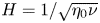
 through $H=1/\sqrt {\eta _{0}\nu }$
 . Alternatively, we shall consider the mean Hartmann number $\langle H \rangle$
 defined as the average value of $H$
 in the tokamak domain.
Let us first investigate the fate of the temperature field. One may actually think that the introduction of the stationary heat equation in the model would not have any significant effect on the value of $T$ in the bulk, compared with simply maintaining an affine temperature everywhere. Indeed, only convective transport of temperature can make $T$
 differ from the Laplace equation solutions. Because poloidal speed was typically very low in previous simulations (Oueslati et al. Reference Oueslati, Bonnet, Minesi, Firpo and Salhi2019), this would seem to suggest a rather limited effect. Figure 1 partly confirms this intuition. For $H = 10$
 , convection is clearly not visible globally. Yet, for $H = 10^5$
 , the temperature profile happens to be deviated by convective effects, meaning that, in this case, poloidal flows are sufficient to provide some heat transport. One observes there some tendency for a temperature homogenization in the tokamak core at large $H$
 .
Temperature profiles (in eV units) for $\Delta T = 10$ and Hartmann numbers (a) $H = 10$
 , (b) $H = 10^5$
 .

Our main interest is to examine the impact of the inhomogeneity of the heating on the steady-state plasma toroidal speed. In the present study, this generation of the toroidal flow is essentially due to viscous effects, as emphasized in the seminal study (Montgomery et al. Reference Montgomery, Bates and Li1997), meaning that, in the Navier–Stokes equation, the toroidal contribution of the $\boldsymbol {\omega } \times \boldsymbol {v}$ term increases with $H$
 while remaining negligible in front of the toroidal contribution of the $\boldsymbol {J} \times \boldsymbol {B}$
 term, that is almost independent on $H$
 .
Figure 2 represents the root mean square (r.m.s.) value of the toroidal velocity field as a function of the mean Hartmann number $\langle H \rangle$ for $\Delta T = 1$
 in Alfvèn units. The numbers $M$
 label different meshes. Up to $\langle H \rangle \times 10^{6}$
 , only one curve can be seen, which means that the simulations yield identical results no matter what mesh is used, illustrating the numerical robustness of the code (see also Appendix B for a discussion on numerical issues at large Hartmann numbers). For reference, the curve corresponding to a uniform temperature on the border ($\Delta T =0$
 ) is also plotted. At any given mean Hartmann number, one observes that the r.m.s. toroidal speed is larger in the inhomogeneous heating case than for constant temperature with a difference increasing with $\langle H \rangle$
 . Figures 3 and 4 show velocity profiles that depart from previous constant temperature results (Oueslati et al. Reference Oueslati, Bonnet, Minesi, Firpo and Salhi2019) as the Hartmann number increases. One observes that the toroidal velocity field goes from being almost odd with respect to the midplane at $H=10$
 to being almost even at $H=10^{5}$
 with a net toroidal flow. The toroidal velocity in itself, although higher than in previous cases, is not particularly impressive at these Hartmann numbers. It is rather the rate at which the velocity increases with $\langle H \rangle$
 , as shown on figure 2, that catches our interest.
The r.m.s. value of $v_{\varphi }$ (in Alfvèn velocity $v_{{A}}$
 units) depending on the mean Hartmann number $\langle H \rangle$
 for $\Delta T = 0$
 and $\Delta T = 1$
 using different mesh sizes (labelled by the number of vertices on the edge of the domain).

Toroidal velocity field $v_{\varphi }$ in Alfvèn velocity $v_{{A}}$
 units with $\Delta T =1$
 for (a) $H = 10$
 and (b) $H = 100$
 .

Toroidal velocity field $v_{\varphi }$ in Alfvèn velocity $v_{{A}}$
 units with $\Delta T =1$
 for (a) $H = 10^3$
 and (b) $H = 10^5$
 .

We now attempt to map the results of the simulations for different $\Delta T$ , even if the largest $\Delta T$
 values may be physically unrealistic. One of our objectives is to obtain faster flows than were previously possible for a uniform temperature. The mean quadratic (r.m.s.) toroidal velocities for different edge temperature gradients are presented in figure 5 for a toroidal free-slip boundary condition and figure 6 for a toroidal no-slip boundary condition. The toroidal free-slip boundary condition allows somehow higher speeds to be reached than the no-slip one for a given $\langle H \rangle$
 which is visible from a comparison between figures 5 and 6. Otherwise, the general behaviour of the curves in both plots is quite similar. The toroidal free-slip boundary condition has been taken in our simulations unless otherwise stated. As expected, for a given $\Delta T$
 , the toroidal velocity always increases with $\langle H \rangle$
 , as the viscous dissipation diminishes. Moreover, the mean value of $\eta$
 has an easily identifiable effect on velocity: for low Hartmann numbers, the more intense the heating, the higher the toroidal velocity. Yet, for higher $\langle H \rangle$
 , the flow behaves differently. The plots corresponding to the most intense heatings are rapidly saturating: the slope of $\langle v_{\varphi } \rangle _{\mathrm {rms}}$
 becomes small compared with simulations with less heating and the greatest temperature gradients do not yield the fastest flows. Conversely, curves with softer heating follow a linear regime on figure 6 over a large band of Hartmann numbers, with a slope equal to 2 (in the log-log scale). This corresponds to $\langle v_{\varphi } \rangle _{\mathrm {rms}}$
 being proportional to $\langle H \rangle ^2$
 . This slope is steeper than what could be achieved without heating, and it provides a physically interesting regime. However, the higher the temperature gradient, the sooner this regime ends (in terms of $\langle H \rangle$
 ). In order to quantify these effects, the instantaneous slope $\beta (\langle H \rangle , \Delta T) \equiv \partial (\log \langle v_{\phi } \rangle _{\mathrm {rms}})/ \partial (\log \langle H \rangle )$
 has been plotted on figure 7. In the infinite viscosity limit, corresponding to $\langle H \rangle \rightarrow 0$
 , one recovers that the quadratic mean (or r.m.s.) of the toroidal velocities scales as $\langle H \rangle ^{4}$
 (i.e. $\beta \rightarrow 4$
 ) which was analytically predicted for $\Delta T=0$
 in Kamp, Montgomery & Bates (Reference Kamp, Montgomery and Bates1998). One observes the aforementioned intermediate scaling $\langle H \rangle ^{2}$
 with $\beta$
 plateauing about 2 for moderate heating gradients compared with an intermediate scaling with $\beta$
 approximately 3/2 taking place for $\Delta T \rightarrow 0$
 .
The r.m.s. of the toroidal velocity, $\langle v_{\varphi } \rangle _{\mathrm {rms}}$ , (in Alfvèn velocity $v_{{A}}$
 units) as a function of $\langle H \rangle$
 for different values of $\Delta T$
 .

The r.m.s. of the toroidal velocity, $\langle v_{\varphi } \rangle _{\mathrm {rms}}$ , (in Alfvèn velocity $v_{{A}}$
 units) as a function of $\langle H \rangle$
 for different values of $\Delta T$
 . Here the toroidal no-slip condition ($u_{4}=0$
 on the border of the plasma domain) is used.

Instantaneous slopes of the logarithm of the r.m.s. of the toroidal velocity, $\langle v_{\varphi } \rangle _{\mathrm {rms}}$ , as a function of the logarithm of $\langle H \rangle$
 for different values of $\Delta T$
 for the toroidal no-slip results plotted in figure 6.

All this makes it not easy to point out an optimal set of parameters in order to reach fast-flow states, especially since the real, physical value of the viscosity coefficient – and therefore the Hartmann number – remains unknown. Besides, simulations with high $\Delta T$ present little physical interest besides drawing a general picture of the situation, yet moderate $\Delta T$
 -values provide some interesting results: as seen on figures 2, 5 and 6, several orders of magnitude in velocity can be gained over the uniform-temperature simulations. On the basis of figure 1, one may propose an explanation for the dual role played by the temperature gradient $\Delta T$
 . Indeed, when both $\Delta T$
 and $\langle H \rangle$
 are large, the effective temperature field will tend to homogenize in the core of the tokamak. The effect of this homogenization is to make less effective or to counterbalance the symmetry breaking induced primarily by the inhomogeneous heating imposed by boundary conditions. One may then understand that there exists some optimum in the choice of $\Delta T$
 in terms of the maximization of mean toroidal plasma speed and that a ‘moderate’ up-down temperature gradient $\Delta T$
 may eventually be more efficient than a large $\Delta T$
 to make plasma rotate in the large $\langle H \rangle$
 values relevant to fusion tokamak plasmas.
Finally, it may be interesting to capture the effect of the additional, vertically ($y$ )-inhomogeneous, heating in terms of the toroidal plasma rotation. Figure 8 represents the ratios $\langle v_{\varphi } \rangle _{\mathrm {rms}}(\Delta T \neq 0)/\langle v_{\varphi } \rangle _{\mathrm {rms}}(\Delta T=0)$
 as a function of the Hartmann number at the bottom of the tokamak, $H$
 , for several values of $\Delta T$
 . This indicates that, for large fusion-relevant values of $H$
 (H between $10^6$
 and $10^8$
 ), the toroidal plasma rotation is maximized by an optimal, moderate, differential heating corresponding to a $\Delta T$
 of order one. At those large fusion-relevant values of $H$
 , numerical simulations become challenging due to the emergence of a boundary layer having a thickness decreasing with $H$
 . This is visible on the plots of the toroidal velocity profile of figure 9. A point on the numerical results at large $H$
 is presented in Appendix B.
For the same data as in figure 6, plots of the ratio $\langle v_{\varphi } \rangle _{\mathrm {rms}}(\Delta T \neq 0)/\langle v_{\varphi } \rangle _{\mathrm {rms}}(\Delta T=0)$ as a function of $H$
 (Hartmann number at the bottom of the tokamak) for different values of $\Delta T$
 .

Profiles of the toroidal velocity field (in Alfvèn velocity $v_{{A}}$ units) in the case of the toroidal no-slip boundary condition for $\Delta T=0.1$
 and large-$H$
 values equal to (from a–c) $2\times 10^{6}$
 , $5\times 10^{6}$
 and $8\times 10^{6}$
 . Colours are varying with the relative magnitude of $v_{\varphi }$
 for better visualization.

4. Spatial symmetry of solutions
4.1. Preliminary remarks
In order to characterize more precisely the flow modes described earlier, we shall now study the symmetry of solutions with respect to the tokamak horizontal $y=0$ midplane. By introducing an inhomogeneous heating along the vertical $y$
 axis, the up-down symmetry of the problem has been broken. For the uniform-temperature problem, symmetry properties were studied in Oueslati & Firpo (Reference Oueslati and Firpo2020) and the toroidal velocity field was shown to be naturally antisymmetric, i.e. an odd function of $y$
 .
In the present simulations, for high Hartmann numbers we obtain some rather symmetric profiles (see e.g. Figure 4) in stark contrast to the non-heated case. This happens to be a somewhat paradoxical situation since breaking the symmetry of the problem seems to make the solutions go from antisymmetry to symmetry, rather than merely eliminating any symmetry properties. Nevertheless, the picture is more intricate as for instance, in the case of intense heating, there are no longer any obvious symmetry properties for high enough Hartmann numbers (see figure 10).
Toroidal velocity field $v_{\varphi }$ for $\Delta T = 50$
 and $H = 100$
 .

4.2. Symmetry analysis
To go beyond the aforementioned qualitative observations and obtain more precise information, one must quantitatively characterize the symmetry or antisymmetry of our solutions. To that end, we consider the $L^2$ norm of the symmetric and antisymmetric parts of the toroidal velocity. Defining by $\varOmega$
 the tokamak cross-section and by $S_{\varOmega }\equiv \int _{\varOmega }\,\mathrm {d}x\, \mathrm {d}y$
 its surface, we put

and

One has the identity

which leads us to introduce a symmetry argument, $\chi$ , given by $\chi \equiv \arctan ( V_{\mathrm {sym}}/ V_{\mathrm {anti}} )$
 . This scalar quantity allows us to easily visualize the balance between symmetry and antisymmetry in a given velocity field. This argument does not depend on the norm of the velocity itself (which can vary by many orders of magnitude) and it is valued between $0$
 and ${\rm \pi} /2$
 . For simulations with uniform temperature, we get $\langle v_{\varphi }\rangle _{\mathrm {rms}} = V_{\mathrm {anti}}$
 and $V_{\mathrm {sym}}=0$
 , and therefore the symmetry argument is $\chi =0$
 .
4.3. Link between velocity and symmetry
Figures 11 and 12 show a transition from antisymmetry to symmetry in the case $\Delta T = 0.1$ as the Hartmann number increases. For low Hartmann numbers, the toroidal velocity profile is indistinguishable from that of the simulations done with uniform temperature: it appears to be antisymmetric and the two plots of $\langle v_{\varphi } \rangle _{\mathrm {rms}}$
 are identical. We then have a rather abrupt transition around $H = 1000$
 , and the symmetry argument tends towards ${\rm \pi} /2$
 (total up-down symmetry) for large $H$
 . What catches our interest is that the transition from antisymmetry to symmetry occurs simultaneously with the separation of the r.m.s. velocities of the homogeneous and non-homogeneous heating cases; it appears that the flow goes from a uniform-temperature-like state to a faster, more symmetric state.
Toroidal velocity field $v_{\varphi }$ for $\Delta T = 0.1$
 and (a) $H=10$
 , (b) $H = 10^5$
 .

(a) Symmetry argument $\chi =\arctan ( V_{\mathrm {sym}}/V_{\mathrm {anti}} )$ for $\Delta T=0.1$
 ; (b) $\langle v_{\varphi }\rangle _{\mathrm {rms}}$
 for $\Delta T$
 equal to 0 and 0.1 as a function of $\langle H \rangle$
 .

This phenomenon is also encountered for other values of $\Delta T$ , although the transition occurs at different $H$
 . The plots do not reach sufficiently high Hartmann numbers to feature the asymptotic symmetry, due to limitations in computing capabilities (somewhat paradoxically, for small values of $\Delta T$
 , the less intense the inhomogeneity of the heating, the more numerically demanding the code becomes) as visible on figure 13.
(a) Toroidal velocity $v_{\varphi }$ field for $H = 10^4$
 and $\Delta T = 0.01$
 ; (b) symmetry argument $\chi =\arctan ( V_{\mathrm {sym}}/V_{\mathrm {anti}} )$
 for $\Delta T=0.01$
 ; (c) $\langle v_{\varphi }\rangle _{\mathrm {rms}}$
 for $\Delta T$
 equal to 0 and 0.01 as a function of $\langle H \rangle$
 .

For higher values of $\Delta T$ , however, other phenomena occur at high $H$
 as depicted in figure 14. After transitioning towards symmetry, this new behaviour (that cannot be easily interpreted in terms of symmetry) seems to be correlated with the velocity saturation mentioned earlier.
(a) Symmetry argument $\chi =\arctan ( V_{\mathrm {sym}}/V_{\mathrm {anti}} )$ for $\Delta T=1$
 ; (b) $\langle v_{\varphi }\rangle _{\mathrm {rms}}$
 for $\Delta T$
 equal to 0 and 1 as a function of $\langle H \rangle$
 .

5. Conclusions
In this study, the impact of a space-inhomogeneous heating on steady flows has been considered. In the limit of small Hartmann numbers, the r.m.s. toroidal velocity has been shown to display the same scaling as that of the uniform-temperature solution with $\langle v_{\varphi }\rangle _{\mathrm {rms}}\propto \langle H \rangle ^{4}$ , with an up-down antisymmetry of the toroidal velocity field. However, it appears that the uniform-temperature, purely antisymmetric solution is unstable with respect to finite-temperature perturbations. Actually, no matter how small the temperature gradient $\Delta T$
 , for sufficiently high $H$
 , the steady-state solution drastically diverges from it. In this sense, the limit $\Delta T \rightarrow 0$
 is singular. Interestingly, for non-vanishingly small $\Delta T$
 , some scaling law $\langle v_{\varphi }\rangle _{\mathrm {rms}}\propto \langle H \rangle ^{2}$
 (faster than the uniform-temperature case) has been uncovered within some range of large values of the Hartmann number which depends on $T$
 ; it coincides with a rather up-down symmetric profile of the toroidal velocity field. Eventually, it happens that perturbing the temperature boundary conditions at finite $H$
 allows much higher flow speeds to be obtained at high Hartmann numbers than the uniform-temperature case. One may, of course, question the somewhat arbitrary choice of using a linear ansatz for the boundary temperature profiles: since the system is strongly nonlinear, other choices may yield different results. The efficiency of the linear profiles seems to lie in its ability to break vertical symmetry in the domain, which enables a divergence from the antisymmetric solution. Finally, one may interpret the coexistence of both symmetric and antisymmetric solutions in the high $H$
 limit as the signal of a bifurcation in the sense of hydrodynamics.
Acknowledgements
The authors thank N. Minesi, T. Bonnet, R. Guillot and A. Salhi for their fruitful discussions.
Editor Steve Tobias thanks the referees for their advice in evaluating this article.
Funding
Ms H. Oueslati thanks the University of Tunis El Manar and the Ministry of Higher Education and Scientific Research of Tunisia for funding. This work has been performed in the frame of the FR-FCM (Fédération nationale de Recherche Fusion par Confinement Magnétique – ITER).
Declaration of interests
The authors report no conflict of interest.
Appendix A. Equations in terms of scalar fields
The reader is referred to Kamp & Montgomery (Reference Kamp and Montgomery2004) for a detailed derivation of the system of coupled differential equations to be solved in the case of a constant resistivity for computing visco-resistive MHD steady states with realistic tokamak driving terms. Indeed, one takes into account the drives induced by an external (thus curl-free) toroidal magnetic field and by a toroidal loop voltage that serves to produce the toroidal current density field that is the source of the poloidal magnetic field. When resistivity is no longer constant as in the present study, the equation for $B_{\varphi }$ is modified. Taking the curl of Ohm's law gives, using $\boldsymbol {\nabla }\times \boldsymbol {E}=\boldsymbol {0}$
 ,

We have

and

We have similarly

and

Using the axisymmetry implying, e.g. $\boldsymbol {\nabla }\chi \boldsymbol {\cdot } \boldsymbol {\nabla } \varphi =\boldsymbol {\nabla }\psi \boldsymbol {\cdot } \boldsymbol {\nabla }\varphi =0$ and $( \boldsymbol {\nabla }\varphi ) ^{2}=r^{-2}$
 , a straightforward calculation gives

The toroidal projection of the curl of this yields

We have

giving

Then

Consequently, we have

In the previous equations, we have made use of the second-order elliptic operator ${\Delta} ^{\ast }$ defined by

Let us define the rescaled variables $x=r/r_{0}$ , $y=z/r_{0}$
 and introduce notations extending that of Kamp & Montgomery (Reference Kamp and Montgomery2003b), namely


where $I_{b}=r_{0}B_{0}$ . Let us define the Poisson bracket of two functions $u$
 and $v$
 with respect to the variables $x$
 and $y$
 as

The system of equations to be solved reads finally


We have introduced the constants $\alpha =\eta _{0}r_{0}^{3/2}$ and $I_{e}=r_{0}^{2}E_{0}$
 with $\eta _{0}\equiv \eta (T_{0})$
 . The boundary conditions chosen in the numerics are $u_{1}=u_{2}=u_{5}=0$
 , $u_{3}=1$
 . Here, $u_{7}$
 is an affine function of $y$
 . As for $u_{4}$
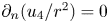
 , we take either (in almost all simulations) the condition $\partial _{n}(u_{4}/r^2)=0$
 corresponding to a free-slip (also called shear-stress free) in the toroidal direction or (exceptionally) $u_{4}=0$
 corresponding to a no-slip toroidal condition. The reader is referred to Oueslati & Firpo (Reference Oueslati and Firpo2020) for a detailed discussion on boundary conditions.
Appendix B. Focus on large-$H$ numerical results

Obtaining robust numerical results at values of the Hartmann numbers as large as $10^6$ to $10^8$
 is important because these are the values expected to be relevant for fusion tokamak plasmas. The essential difficulty in attaining these values lies in the numerical treatment of boundary layers having a thickness decreasing with $H$
 (Kamp & Montgomery Reference Kamp and Montgomery2003a) as illustrated on figure 9. In previous publications (Oueslati et al. Reference Oueslati, Bonnet, Minesi, Firpo and Salhi2019; Oueslati & Firpo Reference Oueslati and Firpo2020), we used a mesh refinement on the border of the computational domain $\varOmega$
 . So doing, we have been able to obtain numerical results that produced values of $\langle v_{\varphi } \rangle _{\mathrm {rms}}$
 that were reasonably independent of the accessible number of mesh triangles. In more mathematical terms, the results had some reasonable stability in the $L^{2}$
 -norm for $v_{\varphi }$
 up to $H=10^{7}$
 depending on boundary conditions. In this work, we have been able to improve the numerical space resolution of some FreeFem++ simulations by decreasing the minimum edge size parameter in the mesh refinement due to more powerful computing facilities. This allows the numerical robustness of the code in the large-$H$
 fusion-relevant range to be addressed more rigorously. An example of improving the precision of the results by refining the mesh on the computational domain is given in figures 15 and 16.
Two different meshes of the tokamak cross-section domain. Panel (a) allows the minimum edge size to be 0.004 where this is equal to 0.002 in panel (b).

For $H=8\times 10^{6}$ , $\Delta T=0.1$
 and for $v_{\varphi }=0$
 on $\partial \varOmega$
 , comparison between the toroidal velocity field (in Alfvèn velocity $v_{{A}}$
 units) obtained using (a) the mesh of figure 15(a) and (b) the more refined mesh of figure 15(b). The r.m.s. of $v_{\varphi }$
 i.e. $\|v_{\varphi }\|_{L^{2}}$
 differs by less than some percentage between the two cases. Both plots have been obtained using the command ListPlot3D of Mathematica$^{\circledR}$
 (there is no artificial smoothing).

The proper mathematical method to assess the numerical robustness of finite-element computations is to consider a series of regular meshes and show the convergence of the results as the mesh size tends to zero. Consequently, as the number of triangles covering the domain $\varOmega$ tends to infinity, one needs to observe the $L^{2}$
 convergence of $v_{\varphi }$
 . Figure 17 gives a qualitative observation that this does take place with (and up to) $H=10^{7}$
 . There is, moreover, only a few percentage discrepancy between the various r.m.s. values of $v_{\varphi }$
 .
For $H=10^{7}$ and $\Delta T=0.1$
 (giving $\langle H \rangle \simeq 1.04 \times 10^{7}$
 ), and for $v_{\varphi }=0$
 on $\partial \varOmega$
 , the r.m.s. of $v_{\varphi }$
 i.e. $\|v_{\varphi }\|_{L^{2}}$
 (in Alfvèn velocity $v_{{A}}$
 units) obtained numerically is plotted as a function of the number of triangles of the mesh. The dispersion of the results on the left part is due to the fact that we do not use a single series of regular meshes.


 Open access

