2.1 Equations of the model

We employ the Hybrid Vlasov–Maxwell (HVM) model, where protons are kinetically described by the Vlasov equation, while electrons are treated as a massless fluid. As usual in the HVM approach, we assume that the electron fluid is isothermal: $T_{e}=\text{const}$. The equations describing the HVM model, in dimensionless units, are the following:

(2.1)$$\begin{eqnarray}\displaystyle & \displaystyle {\displaystyle \frac{\unicode[STIX]{x2202}f}{\unicode[STIX]{x2202}t}}+\boldsymbol{v}\boldsymbol{\cdot }\unicode[STIX]{x1D735}f+(\boldsymbol{E}+\boldsymbol{v}\times \boldsymbol{B})\boldsymbol{\cdot }{\displaystyle \frac{\unicode[STIX]{x2202}f}{\unicode[STIX]{x2202}\boldsymbol{v}}}=0, & \displaystyle\end{eqnarray}$$

(2.2)$$\begin{eqnarray}\displaystyle & \displaystyle \boldsymbol{E}=-\boldsymbol{u}\times \boldsymbol{B}+{\displaystyle \frac{1}{n}}(\,\boldsymbol{j}\times \boldsymbol{B})-{\displaystyle \frac{1}{n}}\unicode[STIX]{x1D735}p_{e}, & \displaystyle\end{eqnarray}$$

(2.3)$$\begin{eqnarray}\displaystyle & \displaystyle {\displaystyle \frac{\unicode[STIX]{x2202}\boldsymbol{B}}{\unicode[STIX]{x2202}t}}=-\unicode[STIX]{x1D735}\times \boldsymbol{E};\quad \boldsymbol{j}=\unicode[STIX]{x1D735}\times \boldsymbol{B};\quad p_{e}=nT_{e}, & \displaystyle\end{eqnarray}$$

where, $f=f(\boldsymbol{x},\boldsymbol{v},t)$ is the proton distribution function (DF), $n=n(\boldsymbol{x},t)$ and $\boldsymbol{u}=\boldsymbol{u}(\boldsymbol{x},t)$ are the density and proton bulk velocity, respectively,

(2.4a,b)$$\begin{eqnarray}n(\boldsymbol{x},t)=\int f(\boldsymbol{x},\boldsymbol{v},t)\,\text{d}^{3}\boldsymbol{v};\quad \boldsymbol{u}(\boldsymbol{x},t)={\displaystyle \frac{1}{n(\boldsymbol{x},t)}}\int \boldsymbol{v}f(\boldsymbol{x},\boldsymbol{v},t)\,\text{d}^{3}\boldsymbol{v}.\end{eqnarray}$$

In the above equations the magnetic field $\boldsymbol{B}$ is normalized to a typical value $\tilde{B}$; the density $n$ is normalized to a typical value ${\tilde{n}}$; velocities $\boldsymbol{v}$ and $\boldsymbol{u}$ are normalized to the typical Alfvén speed $\tilde{c}_{A}=\tilde{B}(4\unicode[STIX]{x03C0}m_{p}{\tilde{n}})^{-1/2}$; the electric field $\boldsymbol{E}$ is normalized to$\tilde{E}=(\tilde{c}_{A}/c)\tilde{B}$; the time $t$ is normalized to the typical proton gyration time $\tilde{\unicode[STIX]{x1D6FA}}_{p}^{-1}$, with $\tilde{\unicode[STIX]{x1D6FA}}_{p}=e\tilde{B}/(m_{p}c)$; space variables are normalized to the typical proton inertial length $\tilde{d}_{p}=\tilde{c}_{A}/\tilde{\unicode[STIX]{x1D6FA}}_{p}$; the current density $\boldsymbol{j}$ is normalized to the value $\tilde{j}=c\tilde{B}/(4\unicode[STIX]{x03C0}\tilde{d}_{p})$; and the electron temperature $T_{e}$ is normalized to the typical temperature $\tilde{T}=\tilde{B}^{2}/(4\unicode[STIX]{x03C0}\unicode[STIX]{x1D705}_{B}{\tilde{n}})$. In what follows, all the results will be expressed in terms of the above-defined dimensionless variables.

The system of equations (2.1)–(2.4) is solved by means of the HVM numerical algorithm (Valentini et al. Reference Valentini, Trávníček, Califano, Hellinger and Mangeney2007). The spatial domain is two-dimensional and is defined by $D_{\boldsymbol{x}}=\{(x,y)\}=[0,L]\times [0,L]$, $L=16\unicode[STIX]{x03C0}$ being the domain size, while the 3-D domain in the velocity space is defined by $D_{\boldsymbol{v}}=\{(v_{x},v_{y},v_{z}),-7v_{\text{th},p}\leqslant v_{i}\leqslant 7v_{\text{th},p},i=x,y,z\}$, where $v_{\text{th},p}$ is a typical dimensionless proton thermal speed, defined in the next section. Periodic boundary conditions are imposed on the boundaries of the spatial domain $D_{\boldsymbol{x}}$ for all quantities, while the DF is imposed to vanish at the boundaries of the velocity–space domain $D_{\boldsymbol{v}}$. More details on the numerical method can be found in Valentini et al. (Reference Valentini, Trávníček, Califano, Hellinger and Mangeney2007).

2.2 Stationary configuration

The stationary configuration corresponds to a magnetized plasma with a shearing flow, where the magnetic field $\boldsymbol{B}_{0}$ is uniform and directed parallel to the sheared bulk velocity $\boldsymbol{u}_{0}$. Building such kind of configuration is straightforward in the case of MHD, but it is more complex within a kinetic approach. Explicit solutions have been found by Roytershteyn & Daughton (Reference Roytershteyn and Daughton2008) in the fully kinetic case, and by Malara, Pezzi & Valentini (Reference Malara, Pezzi and Valentini2018) within the HVM approach. Here, we will use the solution of the HVM case, which is briefly described in the following; more details can be found in Malara et al. (Reference Malara, Pezzi and Valentini2018).

We consider a Cartesian reference frame, where the uniform magnetic field is directed along the $y$ axis: $\boldsymbol{B}_{0}=B_{0}\boldsymbol{e}_{y}$ ($B_{0}=1$ in code units), while the bulk velocity is directed along $y$ as well, but varies in the $x$ direction: $\boldsymbol{u}_{0}=u_{0}(x)\boldsymbol{e}_{y}$, $\boldsymbol{e}_{x}$ and $\boldsymbol{e}_{y}$ being the unit vectors in the $x$ and $y$ directions, respectively. The electric field is vanishing: $\boldsymbol{E}_{0}=0$, therefore protons move along helical trajectories, with the helix axis parallel to the $y$ direction. In this configuration, the motion invariants are: the particle kinetic energy $\mathscr{E}$, the parallel velocity component $v_{y}$ and the $x$-position of the particle guiding centre $x_{c}=x-v_{z}/\unicode[STIX]{x1D6FA}_{p}$, ($\unicode[STIX]{x1D6FA}_{p}=1$ in code units). We build a proton DF $f_{0}$ in terms of the above constants of motion, which is similar to a Maxwellian, shifted in the $v_{y}$ direction by a quantity $U(x_{c})$, where $U(\cdot )$ is an arbitrary function which contributes to determine the profile $u_{0}(x)$ of the bulk velocity. The explicit form of the DF is given by the following combination of the motion constants:

(2.5)$$\begin{eqnarray}f_{0}(x,v_{x},v_{y}.v_{z})=\frac{n_{0}}{(2\unicode[STIX]{x03C0})^{3/2}v_{\text{th}0,p}^{3}}\exp \left[-\frac{1}{2v_{\text{th}0,p}^{2}}\left\{v_{x}^{2}+\left[v_{y}-U\left(x-\frac{v_{z}}{\unicode[STIX]{x1D6FA}_{p}}\right)\right]^{2}+v_{z}^{2}\right\}\right],\end{eqnarray}$$

where the meaning of the constants $n_{0}$ and $v_{\text{th}0,p}$ is specified below. Since $f_{0}$ is expressed only in terms of single-particle motion constants, it is an exact stationary solution of the Vlasov equation (2.1), provided that both $\boldsymbol{B}$ and $\boldsymbol{E}$ remain stationary. Calculating the moments of the DF, we find that the associated density is uniform: $n\equiv \int f_{0}\,\text{d}^{3}\boldsymbol{v}=n_{0}=\text{const}.$, and the bulk velocity is directed along $y$: $u_{0x}=u_{0z}=0$. As a consequence, since $T_{e}=\text{const.}$, we have $\unicode[STIX]{x1D735}p_{e}=0$ (third equation (2.3)). Moreover, with $\boldsymbol{u}_{0}$ parallel to $\boldsymbol{B}$, and $\boldsymbol{B}$ uniform, the generalized Ohm’s law (2.2) implies that $\boldsymbol{E}=0$. In turn, this gives a vanishing time derivative of $\boldsymbol{B}$ (Faraday’s law (2.3)). In summary, both the electric and magnetic fields are stationary and the considered configuration represents a stationary solution for the entire set of HVM equations.

In the particular case where the function $U(\cdot )$ is constant, the expression (2.5) reduces to a shifted Maxwellian; therefore, the constant $v_{\text{th}0,p}$ can be interpreted as the thermal velocity of protons in regions far from the velocity shear, where the distribution function (2.5) approaches a shifted Maxwellian. The only non-vanishing bulk velocity component $u_{0y}$ depends on the function $U(\cdot )$ through the expression (Malara et al. Reference Malara, Pezzi and Valentini2018)

(2.6)$$\begin{eqnarray}u_{0y}(x)=\frac{1}{(2\unicode[STIX]{x03C0})^{1/2}v_{\text{th}0,p}}\int _{-\infty }^{\infty }U\left(x-\frac{v}{\unicode[STIX]{x1D6FA}_{p}}\right)\exp \left(-\frac{v^{2}}{2v_{\text{th}0,p}^{2}}\right)\text{d}v.\end{eqnarray}$$

Therefore, the bulk velocity profile $u_{0y}(x)$ does not coincide with $U(x)$, except in the case $U(x)=U_{0}=\text{const}.$, when $u_{0y}(x)=U_{0}$. In general, denoting with $\unicode[STIX]{x1D6E5}$ the scale of variation of the function $U(\cdot )$, it can be shown that $u_{0y}(x)\simeq U(x)$, if $\unicode[STIX]{x1D6E5}\gg R_{p}$, where $R_{p}$ is the dimensionless proton Larmor radius. Considering the opposite limit $\unicode[STIX]{x1D6E5}<R_{p}$, it can also be shown that, in the considered configuration, the actual width of a velocity shear cannot be smaller than the proton Larmor radius (Malara et al. Reference Malara, Pezzi and Valentini2018).

In our case, we used the following form for the function $U(x)$:

(2.7)$$\begin{eqnarray}U(x)=U_{0}\left[\tanh \left(\frac{x-L/4}{\unicode[STIX]{x1D6E5}}\right)-\tanh \left(\frac{x-3L/4}{\unicode[STIX]{x1D6E5}}\right)-1\right],\end{eqnarray}$$

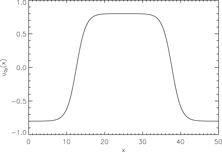
which gives a profile for $u_{0y}(x)$ with two shears localized at $x=L/4$ and $x=3L/4$. The bulk velocity is $u_{0y}\simeq U_{0}$ in the centre $x=L/2$ of the spatial domain, while it is $u_{0y}\simeq -U_{0}$ on the two sides $x=0$ and $x=L$. In particular, we used the following values for the above parameters: $U_{0}=0.8$, $\unicode[STIX]{x1D6E5}=2.5$. The corresponding profile for the bulk velocity $u_{0y}(x)$ is shown in figure 1. The value of $U_{0}$ has been chosen relatively large to reduce the phase-mixing time, and, consequently, the computation time. On the other hand, a large jump $\unicode[STIX]{x1D6E5}u_{y}$ in the bulk velocity across the shear layers can lead to the development of the Kelvin–Helmholtz (KH) instability which would superpose on the wave dynamics. In order to prevent the KH instability developing in our simulations, we have chosen $U_{0}$ sufficiently low to fulfil the condition $\unicode[STIX]{x1D6E5}u_{y}<2c_{A}$. This choice stabilizes the system against the KH instability, at least in the MHD case. In particular, we have chosen $\unicode[STIX]{x1D6E5}u_{y}\simeq 1.6c_{A}$ ($c_{A}=1$ in code units).

Figure 1.

Profile of the stationary-state bulk velocity $u_{0y}$ as a function of $x$.

We notice that in the two shear regions the DF (2.5) departs from a shifted Maxwellian. In particular, the proton temperature is anisotropic: $T_{||}\geqslant T_{\bot }$, where $T_{||}$ and $T_{\bot }$ are the parallel and perpendicular temperature with respect to the magnetic field direction, respectively, and agyrotropy features are also present (Malara et al. Reference Malara, Pezzi and Valentini2018). Far from the velocity shears the proton temperature becomes isotropic and reaches the value $T_{0p}$, corresponding to the asymptotic thermal speed $v_{\text{th}0,p}$.

2.3 Alfvénic perturbation

At the initial time $t=0$ a perturbation is superposed on the above stationary configuration, with properties similar to a linearly polarized large-scale Alfvén wave. Within MHD theory, an Alfvén wave is polarized in the direction perpendicular both to the background magnetic field $\boldsymbol{B}_{0}$ and to the wavevector $\boldsymbol{k}$. In our case, $\boldsymbol{B}_{0}$ is in the $y$ direction, while $\boldsymbol{k}$ varies in time due to phase mixing, but remains in the $x-y$ plane. Therefore, we selected a perturbation polarized along the $z$ direction. We considered a proton DF in the form: $f=f_{0}+f_{1}$, where the perturbed DF has the form of a Maxwellian shifted in the $v_{z}$ direction

(2.8)$$\begin{eqnarray}f_{1}(y,v_{x},v_{y},v_{z})=\frac{n_{1}}{(2\unicode[STIX]{x03C0})^{3/2}v_{\text{th}0,p}^{3}}\exp \left\{-\frac{v_{x}^{2}+v_{y}^{2}+\left[v_{z}-U_{z}(y)\right]^{2}}{2v_{\text{th}0,p}^{2}}\right\},\end{eqnarray}$$

where $U_{z}(y)=\cos (k_{0}y)$, with $k_{0}=2\unicode[STIX]{x03C0}/L$ corresponding to a wavelength $\unicode[STIX]{x1D706}_{y}$ equal to the domain size $L$, and $n_{1}$ constant. We notice that $\unicode[STIX]{x1D706}_{y}\gg d_{p}=1$. Therefore, the initial perturbation can be considered to be in an MHD regime. The total density is uniform and is given by

(2.9)$$\begin{eqnarray}n=\int f_{0}(x,\boldsymbol{v})\,\text{d}^{3}\boldsymbol{v}+\int f_{1}(y,\boldsymbol{v})\,\text{d}^{3}\boldsymbol{v}=n_{0}+n_{1}=\text{const}.\end{eqnarray}$$

This is coherent with the fact that an Alfvén wave does not involve density perturbations. The bulk velocity is given by a weighted average between the stationary-state bulk velocity $\boldsymbol{u}_{0}$ and the bulk velocity associated with the perturbation

(2.10)$$\begin{eqnarray}\boldsymbol{u}(x,y)=\frac{1}{n}\int \boldsymbol{v}f(\boldsymbol{x},\boldsymbol{v})\,\text{d}^{3}\boldsymbol{v}=\frac{n_{0}u_{0y}(x)\boldsymbol{e}_{y}+n_{1}U_{z}(y)\boldsymbol{e}_{z}}{n_{0}+n_{1}}.\end{eqnarray}$$

We have fixed the value $n_{0}=1$, while the parameter $n_{1}$ has been used to determine the amplitude $A_{1}=n_{1}/(n_{0}+n_{1})$ of the initial Alfvénic perturbation.

Table 1.

Values of parameters used in the runs.

In the MHD regime, velocity $\boldsymbol{u}_{1}$ and magnetic field $\boldsymbol{B}_{1}$ fluctuations are related by the expression $\boldsymbol{B}_{1}=\mp (B_{0}/c_{A})\boldsymbol{u}_{1}$, where $c_{A}=1$ is the normalized Alfvén velocity associated with the equilibrium structure and the upper (lower) sign corresponds to waves propagating in the direction of $\boldsymbol{B}_{0}$ (opposite to $\boldsymbol{B}_{0}$). Therefore, we have chosen the magnetic field initial perturbation as

(2.11)$$\begin{eqnarray}\boldsymbol{B}_{1}(y)=-\frac{n_{1}}{n_{0}+n_{1}}U_{z}(y)\boldsymbol{e}_{z}=-A_{1}U_{z}(y)\boldsymbol{e}_{z}.\end{eqnarray}$$

Finally, the initial electric field $\boldsymbol{E}$ is determined by the generalized Ohm’s law (2.2).

3.1 Run 1: small-amplitude perturbation

We start by describing the results obtained in the small-amplitude run (Run 1, $A_{1}\simeq 0.01$). Due to the low value of the wave amplitude, nonlinear effects are negligible and the dynamics is completely dominated by the interaction of the wave with the inhomogeneity determined by the background velocity shear. Therefore, the purpose of this run is to clearly single out inhomogeneity linear effects, such as phase mixing. In the following, the fluctuating part of any quantity $F(\boldsymbol{x},t)$ is defined as $\unicode[STIX]{x1D6FF}F=F-\langle F\rangle _{D_{\boldsymbol{x}}}$, where angular parentheses indicate an average over the spatial domain $D_{\boldsymbol{x}}$.

Figure 2.

Two-dimensional plots in the $x-y$ plane of fluctuating magnetic field components $\unicode[STIX]{x1D6FF}B_{z}$ (a–c) and $\unicode[STIX]{x1D6FF}B_{y}$ (d–f) at three different times: $t=20$ (a,d); $t=60$ (b,e); and $t=80$ (c,f). All plots refer to the low-amplitude run (Run 1).

In figure 2 the fluctuating magnetic field component $\unicode[STIX]{x1D6FF}B_{z}$ is plotted for three different times during the simulation (a–c). At the initial time (not shown), only the $\unicode[STIX]{x1D6FF}B_{z}$ component, corresponding to the initial Alfvénic perturbation, is non-vanishing. The effects of phase mixing on the time evolution of $\unicode[STIX]{x1D6FF}B_{z}$, due to space variations of the bulk velocity $u_{y}$, are clearly visible. The wave propagation velocity $\boldsymbol{v}_{W}$ in the simulation reference frame is the sum of the Alfvén velocity plus the bulk velocity $\boldsymbol{v}_{W}(x)=[c_{A}+u_{y}(x)]\boldsymbol{e}_{y}$. Accordingly, $v_{W}$ is larger in the centre of the spatial domain than on the two sides. As a consequence, initially plane wavefronts are progressively bent in the two velocity shear regions, where the wavevector perpendicular component $k_{x}$ locally increases, while the wavelength decreases. Dispersive effects become effective for wavevectors of the order of $k_{\text{disp}}\simeq d_{p}^{-1}=1$, corresponding to a wavelength $\unicode[STIX]{x1D706}_{\text{disp}}\simeq 2\unicode[STIX]{x03C0}$. At later times in the simulation ($t\gtrsim 60$), the wavelength of the perturbation in the shear regions has decreased to $\unicode[STIX]{x1D706}\sim \unicode[STIX]{x1D706}_{\text{disp}}$. After that time, dispersive effects becomes relevant, at least within the velocity shear regions. In these regions, we observe that the magnetic fluctuation parallel component $\unicode[STIX]{x1D6FF}B_{y}$ (shown in figure 2d–f) increases in time, until reaching values of the same order of $\unicode[STIX]{x1D6FF}B_{z}$ for times $t\geqslant 60$. In the MHD case, where dispersive effects are neglected, the same phase-mixing problem would give a null $\unicode[STIX]{x1D6FF}B_{y}$ for all times, implying that the generation of $\unicode[STIX]{x1D6FF}B_{y}$ is only caused by non-MHD dispersive effects. In fact, $\unicode[STIX]{x1D6FF}B_{y}$ grows only in the two shear regions, where the wavelength is small enough to make dispersive effects relevant. In summary, in the velocity shear regions perturbations change their properties: the initial linear Alfvénic polarization is modified by the growth of a parallel component $\unicode[STIX]{x1D6FF}B_{y}$, the wavevector becomes nearly perpendicular ($k_{||}\ll k_{\bot }$) and of the order of the inverse proton Larmor radius. These evidences suggest that the initial Alfvénic perturbation has been locally converted into a KAW.

Figure 3.

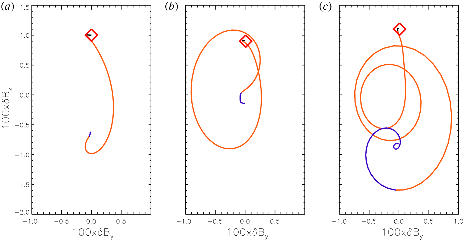
Hodograms in the $\unicode[STIX]{x1D6FF}B_{y}{-}\unicode[STIX]{x1D6FF}B_{z}$ plane, relative to Run 1, at time $t=t_{1}=20$ along the line $L/2\leqslant x\leqslant L$, $y=y_{1}=10$ (a); at time $t=t_{2}=40$ along the line $L/2\leqslant x\leqslant L$, $y=y_{2}=45$ (b); and at time $t_{3}=80$ along the line $L/2\leqslant x\leqslant L$, $y=y_{3}=15$ (c). Black, orange and blue sections are relative to the intervals $L/2\leqslant x<31$, $31\leqslant x<44.5$ and $44.5\leqslant x\leqslant L$, respectively. The red diamonds indicate the point at $x=L/2$.

In order to have a clear identification of the perturbations generated in the velocity shear regions, we have first considered the group velocity $\boldsymbol{v}_{g}$ of the waves. Vásconez et al. (Reference Vásconez, Pucci, Valentini, Servidio, Matthaeus and Malara2015) have shown that in the dispersive MHD all wave modes have a non-vanishing component of $v_{g\bot }$ in the direction perpendicular to $\boldsymbol{B}_{0}$. In particular, for fast magnetosonic waves it is $v_{g\bot }\gtrsim c_{A}$, while for slow magnetosonic and Alfvén waves it is $v_{g\bot }\ll c_{A}$ (Vásconez et al. Reference Vásconez, Pucci, Valentini, Servidio, Matthaeus and Malara2015). In our simulation, we noticed that fluctuations generated in the shear regions propagate also perpendicularly to $\boldsymbol{B}_{0}$, in the direction from the centre to the lateral parts of the spatial domain. However, we verified that the transverse propagation speed is one order of magnitude lower than the Alfvén speed. We conclude that such fluctuations cannot belong to the fast magnetosonic branch.

To further discriminate among slow and Alfvénic fluctuations, we have examined how the orientation of $\unicode[STIX]{x1D6FF}\boldsymbol{B}$ varies along segments parallel to the $x$ axis. In the velocity shear regions these segments are quasi-parallel to the wavevector direction. An example is given in figure 3, where three hodograms are plotted: $\unicode[STIX]{x1D6FF}B_{z}$ versus $\unicode[STIX]{x1D6FF}B_{y}$. These are calculated at three different times: panel (a) refers to the segment defined by $L/2\leqslant x\leqslant L$, $y=y_{1}=10$ at time $t_{1}=20$, panel (b) to the segment $L/2\leqslant x\leqslant L$, $y=y_{2}=45$ at time $t_{1}=40$ and panel (c) to the segment $L/2\leqslant x\leqslant L$, $y=y_{3}=15$ at time $t_{3}=80$. The values $y_{1}$, $y_{2}$ and $y_{3}$ have been chosen such that $\unicode[STIX]{x1D6FF}B_{z}(x=L/2,y_{1,2,3},t_{1,2,3})\simeq \max \{\unicode[STIX]{x1D6FF}B_{z}(x=L/2,y,t_{1,2,3}),\,0\leqslant y\leqslant L\}$. Different sections of the segments are indicated by different colours: black corresponds to the central homogeneous region ($L/2\leqslant x<31$); orange corresponds to the shear region ($31\leqslant x<44.5$); blue corresponds to the lateral homogeneous region ($44.5\leqslant x\leqslant L$). The diamond indicates the values of $\unicode[STIX]{x1D6FF}B_{y}$ and $\unicode[STIX]{x1D6FF}B_{z}$ at the position $x=L/2$.

Figure 3 can be used to determine the polarization of the magnetic perturbation in the $\unicode[STIX]{x1D6FF}B_{y}{-}\unicode[STIX]{x1D6FF}B_{z}$ plane, which is nearly perpendicular to the wavevector in the shear region. Figure 3(a) refers to an early stage of time evolution. At that time, in the shear region (orange section of the curve) the wave polarization is still essentially linear, $z$-aligned, as the initial Alfvén wave. In fact, since the perturbation wavelength in the shear region is still larger than $d_{p}$ (see figure 2a,d), dispersive effects are not large enough to sensibly modify the initial polarization. In the same hodogram we also notice very small variations of the perturbation in the two homogeneous regions (black and blue sections of the curve); this is due to the fact that the hodogram is drawn along a segment that, in the homogeneous regions, is quasi-parallel to wavefronts.

This latter feature is present also at the time $t=40$ (figure 3b), but now the polarization in the shear region (orange section) has turned into clockwise elliptical. This polarization change is due to dispersive effects: they are now more relevant in consequence of the wavelength decrease induced by phase mixing. The same polarization is also found in the shear region at $t=80$ (panel c); the orange section of the curve has a large number of turns with respect to $t=40$ because phase mixing has further decreased the perturbation wavelength. Hodograms calculated along other parallel segments, which are not shown here, display a same behaviour. Considering wave modes within the dispersive MHD (Vásconez et al. Reference Vásconez, Pucci, Valentini, Servidio, Matthaeus and Malara2015), Alfvén and fast magnetosonic waves are both clockwise-elliptically polarized, while slow magnetosonic waves are counter-clockwise polarized. We can therefore exclude that fluctuations generated in the shear regions during system evolution belong to the slow magnetosonic branch.

On the base of the above considerations about polarization and group velocity, the perturbations generated in the velocity shear regions belong to the Alfvén branch, i.e. they are KAWs. Therefore, the phase-mixing mechanism acting in the shear regions gradually triggers a modification from the initial Alfvén wave to KAW fluctuations. Such a transformation takes place gradually in time as the wavevector locally increases and turns, since KAWs belong to the same branch as long-wavelength Alfvén waves. Finally, we notice that a small-amplitude clockwise-elliptically polarized fluctuation is also present in the lateral homogeneous region at time $t=80$ (figure 3c, blue section); due to the non-vanishing $v_{g\bot }$, KAWs do not remain confined in the shear regions but tend to move to the side homogeneous regions.

3.2 Run 2: moderate-amplitude perturbation

When increasing the initial perturbation amplitude, the effects of fluctuating fields on the proton DF become more relevant. In order to study such kinetic effects, and at the same time able to identify the characteristics of the propagation of KAWs during the system evolution, in Run 2 we have chosen a moderately larger amplitude of the initial perturbation $n_{1}=0.1$, corresponding to $A_{1}=0.091$. A larger amplitude would produce significant deformations of the initial equilibrium configuration, making it hard to clearly identify the nature of the transverse fluctuations produced by phase mixing.

The time evolution of magnetic and velocity fields in Run 2 is qualitatively similar to that observed in Run 1 (see figure 2). In particular, the initial Alfvén wave undergoes phase mixing in the two velocity shear regions, locally generating small-scale perturbations with a quasi-perpendicular wavevector. Such perturbations are elliptically polarized in the sense of the Alfvén dispersive branch and slowly expand in the transverse direction, moving outside of the shear regions. Therefore, also in this moderate-amplitude case we can conclude that the initial Alfvén wave is converted into a KAW-like fluctuation by the interaction with the background inhomogeneity due to the velocity shear.

The main differences between the small- and moderate-amplitude cases consist in the modifications of the proton distribution function induced by fluctuations, which are more relevant for Run 2. In order to give a quantitative measure for such a phenomenon, we define the quantity $\unicode[STIX]{x1D702}$

(3.1)$$\begin{eqnarray}\unicode[STIX]{x1D702}(\boldsymbol{x},t)=\frac{1}{n(\boldsymbol{x},t)}\sqrt{\int _{D_{\boldsymbol{v}}}[f(\boldsymbol{x},\boldsymbol{ v},t)-f_{0}(\boldsymbol{x},\boldsymbol{ v})]^{2}\,\text{d}^{3}\boldsymbol{ v}},\end{eqnarray}$$

which represents the $L^{2}$ norm of the departure (in velocity space) between the proton DF $f$, at a position $\boldsymbol{x}$ and time $t$, and the unperturbed DF $f_{0}$ at the same position, normalized to the density. Since $\unicode[STIX]{x1D702}$ is a positive–definite quantity, it is useful to consider also its maximum value calculated over the spatial domain, at a given time $t$: $\unicode[STIX]{x1D702}_{\text{max}}(t)=\max _{D_{\boldsymbol{x}}}\{\unicode[STIX]{x1D702}(\boldsymbol{x},t)\}$. The corresponding position is indicated by $\boldsymbol{x}_{M}(t)$: $\unicode[STIX]{x1D702}(\boldsymbol{x}_{M}(t),t)=\unicode[STIX]{x1D702}_{\text{max}}(t)$.

Figure 4.

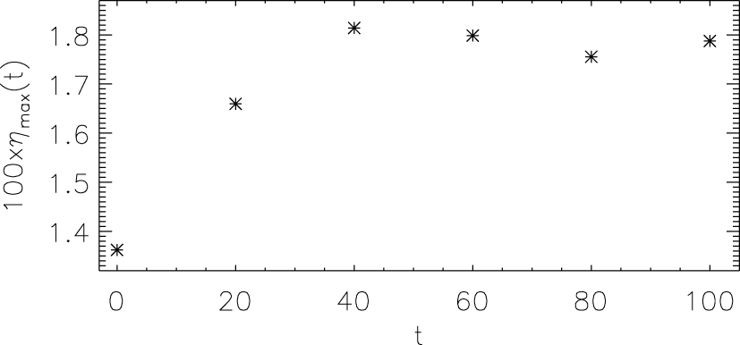
The quantity $\unicode[STIX]{x1D702}_{\text{max}}$ is plotted as a function of time $t$, for the moderate-amplitude run (Run 2).

In figure 4 the quantity $\unicode[STIX]{x1D702}_{\text{max}}(t)$ is plotted as a function of time, for Run 2. At the initial time it is $\unicode[STIX]{x1D702}\neq 0$, due to the DF initial perturbation $f_{1}$ which is superposed on the stationary DF $f_{0}$. We can see that the departure of the DF $f$ from $f_{0}$ slightly increases in time, indicating a progressive modification of the DF due to the effects of the perturbation. The growth of $\unicode[STIX]{x1D702}_{\text{max}}(t)$ saturates at the time $t\simeq 40$, remaining roughly constant after that time. The saturation value is $\unicode[STIX]{x1D702}_{\text{max},\text{sat}}\simeq 1.8\times 10^{-2}$, which is $\simeq 1.3\,\unicode[STIX]{x1D702}_{\text{max}}(t=0)$. The relatively low increase of $\unicode[STIX]{x1D702}_{\text{max}}$ is partially due to the moderate amplitude of the perturbation and partially to the large value of $\unicode[STIX]{x1D6FD}_{p}$. In fact, larger values of $\unicode[STIX]{x1D6FD}_{p}$ corresponds to larger thermal energy in the proton population, when compared to the energy associated with the perturbation. We expect to find an increase of $\unicode[STIX]{x1D702}_{\text{max}}$ more relevant than in the present case, when larger perturbation amplitudes and/or lower $\unicode[STIX]{x1D6FD}_{p}$ are considered.

Figure 5.

Two-dimensional plots of the quantity $\unicode[STIX]{x1D702}(\boldsymbol{x},t)$ in the $x-y$ plane, at time $t=40$ (a) and $t=100$ (b), for the moderate-amplitude run (Run 2). Asterisks indicate the positions where $\unicode[STIX]{x1D702}$ is maximum at the given time.

In figure 5, 2-D plots of $\unicode[STIX]{x1D702}(\boldsymbol{x},t)$ in the $x-y$ plane are shown at times $t=40$ and $t=100$. Asterisks indicate the location $\boldsymbol{x}_{M}$ where $\unicode[STIX]{x1D702}$ attains the maximum value $\unicode[STIX]{x1D702}_{\text{max}}$ for the given time. From this figure we see that the largest departures from the background DF $f_{0}$ are mainly localized within the velocity shear regions, where the smallest wavelengths form in the perturbation. The spatial structure of $\unicode[STIX]{x1D702}(\boldsymbol{x},t)$ appears to be influenced by phase mixing, indicating that the DF is also spatially modulated on a small transverse scale. Therefore, departures from the unperturbed proton DF are strictly related to the generation of small scales, of the order of $d_{p}$.

Figure 6.

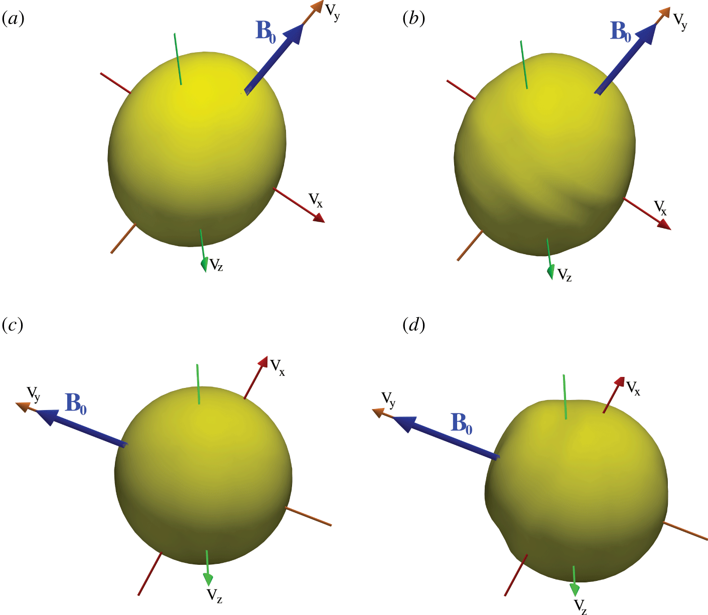
Isosurfaces of the 3-D proton velocity DF $f(\boldsymbol{x}_{M}(t),\boldsymbol{v},t)$ (b,d), and of the stationary DF $f_{0}(\boldsymbol{x}_{M}(t),\boldsymbol{v})$ (a,c), at time $t=40$ (a,b) and $t=100$ (c,d), calculated in the spatial position $\boldsymbol{x}_{M}(t)$ where $\unicode[STIX]{x1D702}=\unicode[STIX]{x1D702}_{\text{max}}$ at the given time. Isosurfaces are relative to the values $f=f_{0}=0.008$. Plots refer to the moderate-amplitude run (Run 2).

Three-dimensional iso-surface plots of the proton DF $f(\boldsymbol{x}_{M}(t),\boldsymbol{v},t)$ in velocity space are shown in figure 6 for $t=40$ and $t=100$, at the position $\boldsymbol{x}_{M}(t)$. For comparison, the unperturbed DF $f_{0}(\boldsymbol{x}_{M}(t),\boldsymbol{v})$ is plotted at the same position (figure 6a,c). The DF modifications become evident by comparing $f$ and $f_{0}$. At time $t=40$, such variations appear as a modulation in form of rings on the considered isosurface (figure 6b), which are co-axial with the direction $y$ of the background magnetic field $\boldsymbol{B}_{0}$, indicated by a blue arrow. We can also notice that the unperturbed DF $f_{0}$ departs from a Maxwellian, the parallel temperature $T_{p||}$ being larger than the perpendicular one $T_{p\bot }$ (Malara et al. Reference Malara, Pezzi and Valentini2018). 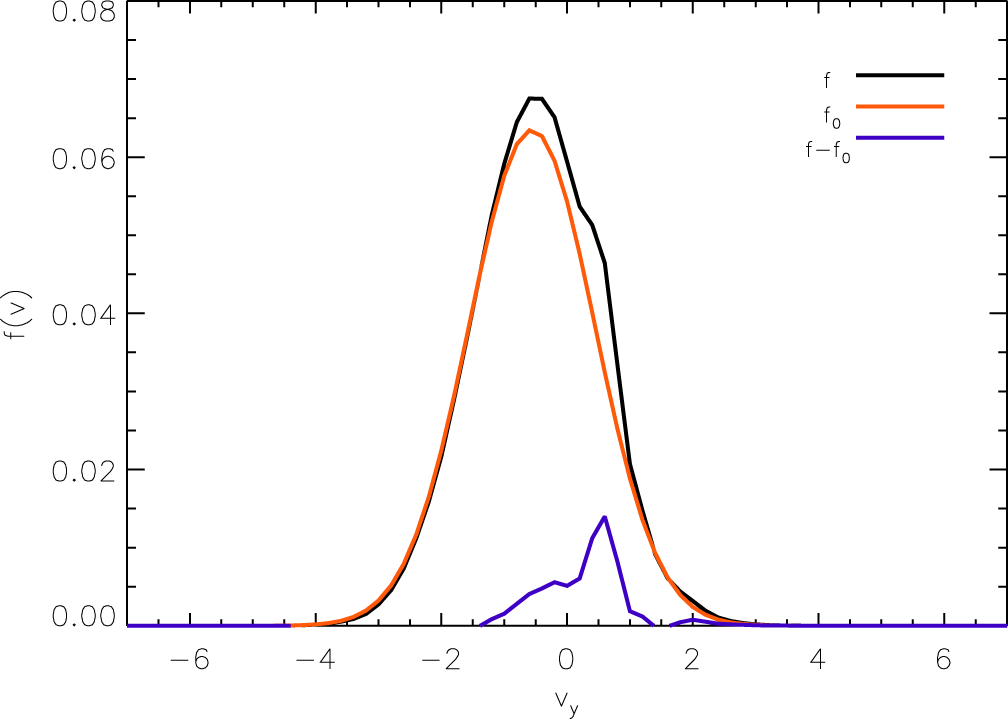At time $t=100$, the DF $f$ shows a peculiar feature where $\unicode[STIX]{x1D702}=\unicode[STIX]{x1D702}_{\text{max}}$; namely, a ‘bulge’ is present in the isosurface (figure 6d), indicating the presence of a sub-population of protons moving along $\boldsymbol{B}_{0}$ faster than the core particles. The existence of this beam of accelerated protons can also be seen in figure 7, where a ‘cut’ of the DF shown in figure 6 for $t=100$ is plotted in velocity space as a function of $v_{y}$, for $v_{x}=v_{z}=0$ (black line). In the same figure, the corresponding profile of the unperturbed DF $f_{0}$ is plotted for comparison (orange line), along with the difference $f-f_{0}$ of the two profiles (blue line). The proton beam is evident also in figure 7; in particular, the difference in velocity between the beam and core population along the $\boldsymbol{B}_{0}$ direction is $\unicode[STIX]{x0394}v_{y}\simeq c_{A}=1$.

Figure 7.

Profiles of the proton distribution functions $f$ (black line), $f_{0}$ (orange line) and of the difference $f-f_{0}$ (blue line) are plotted as functions of $v_{y}$, for $v_{x}=v_{z}=0$, at the space position $\boldsymbol{x}_{M}(t)$ at time $t=100$. Plots refer to the moderate-amplitude run (Run 2).

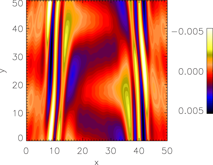
Concerning the origin of the beam, we observe that KAWs are characterized by a component of the electric field $E_{y}$ parallel to the background magnetic field $\boldsymbol{B}_{0}$ (e.g. Hollweg Reference Hollweg1999). Such a component is vanishing in the limit of ideal MHD and can be responsible for particle energization. In figure 8 a 2-D plot of the parallel electric field component $E_{y}$ at the time $t=100$ is shown. Figure 8 shows that $E_{y}$ is localized in the region where the smallest spatial scales are present in the perturbation, while it is negligible outside. Moreover, the spatial pattern of $E_{y}$ is similar to that of other perturbed quantities, and the wavelength in the parallel $y$ direction is $\unicode[STIX]{x1D706}_{||}=2\unicode[STIX]{x03C0}/k_{0}=L$. As a consequence, we can define a sort of electric potential $\unicode[STIX]{x1D719}$, such as $E_{y}=-\unicode[STIX]{x2202}\unicode[STIX]{x1D719}/\unicode[STIX]{x2202}y$. Of course, the dependence of $\unicode[STIX]{x1D719}$ on $y$ is also periodic, with a period equal to $L$. Protons, in their motion, feel this periodic potential and can interact with it. In particular, part of the ion population can remain trapped into the potential well associated with the spatially modulated $E_{y}$ component. For a given particle kinetic energy, this trapping is more probable for protons which move quasi-parallel to $\boldsymbol{B}_{0}$, i.e. with $v_{x}$, $v_{z}\ll v_{y}$; this latter condition corresponds to the cut in figure 7. The potential well co-moves with the wave along the magnetic field with a velocity $\simeq c_{A}$ in the plasma bulk reference frame, which explains why trapped protons have an average velocity of $u_{y}(x)+c_{A}$. This process can account for the formation of the DF features observed in figure 7.

Figure 8.

Two-dimensional plot of the electric field parallel component $E_{y}$ in the $x-y$ plane, calculated at time $t=100$ for the moderate-amplitude run (Run 2).

Indeed, in previous simulations of Alfvén wave phase mixing generated by magnetic field inhomogeneities, the presence of ion beams moving along the magnetic field at the local Alfvén speed has been observed by Vásconez et al. (Reference Vásconez, Pucci, Valentini, Servidio, Matthaeus and Malara2015) and Valentini et al. (Reference Valentini, Vásconez, Pezzi, Servidio, Malara and Pucci2017). These authors have shown that the origin of such beams is the parallel electric field associated with KAW-like fluctuations, generated in the inhomogeneity regions by the phase-mixing mechanism. It is likely that the same physical process is responsible for the creation of suprathermal ion beams also in the case considered in the present paper.