1. Introduction
Accurate prediction of the transition location remains a challenge. Semiempirical methods based on linear instability theory, such as the
 $e^N$
(Smith Reference Smith1956; Van Ingen Reference Van Ingen1956), have been widely used. However, they lack information about the initial amplitude of the instability waves. This amplitude is governed by the ‘receptivity’, the process by which external disturbances give rise to instability waves in the boundary layer (Morkovin Reference Morkovin1969). Understanding receptivity is, therefore, necessary to improve estimates of the transition location. Receptivity can arise from acoustic waves, free stream turbulence (Saric et al. Reference Saric, Reed and Kerschen2002) and there is also receptivity of three-dimensional Tollmien–Schlichting (TS) waves from two-dimensional ones (Crouch Reference Crouch1997; De Paula et al. Reference De Paula, Würz and Medeiros2008, Reference De Paula, Würz, Mendonça and Medeiros2017). Our investigation is concerned only with acoustic receptivity.
Using asymptotic expansions and the triple-deck formalism, Goldstein (Reference Goldstein1983, Reference Goldstein1985) and Ruban (Reference Ruban1984) demonstrated that receptivity is prone to occur in regions of rapid change in the base flow, such as a leading edge or a localised surface irregularity. Note that close to the wall, a Stokes layer is formed due to the acoustic wave. The acoustic receptivity process at the roughness is associated with the Stokes layer (Ruban Reference Ruban1984; Goldstein Reference Goldstein1985; Choudhari & Streett Reference Choudhari and Streett1992). Goldstein (Reference Goldstein1985) was the first to explain this phenomenon theoretically. Choudhari & Streett (Reference Choudhari and Streett1992), Choudhari (Reference Choudhari1993) and Crouch (Reference Crouch1992a
,Reference Crouch
b
) developed the so-called finite Reynolds number theory (FRNT), providing receptivity predictions for moderate Reynolds numbers. Crouch (Reference Crouch1992b
) extended his approach to distributed roughness. The distributed roughness problem was also investigated by Choudhari (Reference Choudhari1993), and, more rigorously, by Wu (Reference Wu2001). These studies explained that, as opposed to localised roughness, the lower branch of the stability loop plays a key role in the receptivity due to distributed roughness. Raposo et al. (Reference Raposo, Mughal and Ashworth2019) proposed a FRNT-based adjoint harmonic linearised Navier–Stokes approach accounting for the non-parallelism of the mean flow which they applied to a localised imperfection. The distributed roughness counter part is presented in Raposo et al. (Reference Raposo, Mughal and Ashworth2018). These adjoint harmonic linearised Navier–Stokes studies also investigated the impact of Mach number (
 $M\!a$
), streamwise position of the roughness and acoustic wave frequency. The effect of a bump on an oncoming TS wave has also been investigated (Wu & Hogg Reference Wu and Hogg2006; Wu & Dong Reference Wu and Dong2016; Xu et al. Reference Xu, Sherwin, Hall and Wu2016; Himeno et al. Reference Himeno, Carvalho and Medeiros2024). This effect is also important and can be related to the acoustic receptivity phenomenon we are investigating, as already pointed out by Dong & Li (Reference Dong and Li2021). We are focusing on the receptivity process only but we take this effect into account as explained in § 3.
Several approaches have been used to measure experimentally the instability waves resulting from the acoustic receptivity (Saric Reference Saric1994; Saric & White Reference Saric and White1998; Monschke et al. Reference Monschke, Kuester and White2016). However, these approaches have limitations associated with robustness, complexity, accuracy or the amount of data required. To overcome these limitations, Placidi et al. (Reference Placidi, Gaster and Atkin2020) developed a novel methodology based on a roughness with adjustable height. Their rig enables acoustic receptivity investigation for both two-dimensional gaps and bumps. Their roughness is rectangular with sharp edges, which are known to be more critical. They obtained good agreement with the linear results for small bump heights and reported a progressively nonlinear behaviour as the bump height exceeded
 $12.6\,\%$
of the local Blasius boundary layer displacement thickness. For the gaps, the experiment indicated an earlier departure from the linear theory. However, they considered that, given the experimental uncertainty and poor signal-to-noise ratio, these findings would have to be confirmed. Theoretical developments put forward by Nayfeh & Ashour (Reference Nayfeh and Ashour1994) showed regions of recirculating flow promote nonlinearity. Work by Bodonyi et al. (Reference Bodonyi, Tadjfar, Welch and Duck1989) and Bodonyi (Reference Bodonyi1990) also suggest that the presence of a separated flow can significantly affect the receptivity behaviour.
Direct numerical simulations (DNS) of acoustic receptivity due to roughness have also been carried out. Würz et al. (Reference Würz, Herr, Wörner, Rist, Wagner and Kachanov2003) conducted DNS of acoustic receptivity for both two-dimensional and isolated three-dimensional roughness elements, as well as experiments for the three-dimensional roughness. Their numerical results fell in the linear regime and the roughness was represented only approximately via a Taylor expansion from the wall. There was good agreement between experiments and numerics for the three-dimensional roughness and good agreement between numerics and the FRNT (Choudhari & Streett Reference Choudhari and Streett1992) for two-dimensional roughness. Their two-dimensional results are further addressed here in § 3.2. De Tullio & Ruban (Reference De Tullio and Ruban2015) performed DNS of the acoustic receptivity of a two-dimensional Gaussian shaped roughness. At a roughness height of approximately 17 % of the local undisturbed Blasius boundary layer displacement thickness, the receptivity dependence on the roughness height becomes superlinear. We use the term ’superlinear’ to indicate that the receptivity amplitude scales with bump height to a power higher than unity. We prefer to avoid the word ’nonlinear’ to prevent misunderstanding with nonlinear behaviour of the TS waves. This term was used by Kurz & Kloker (Reference Kurz and Kloker2014). This threshold is somewhat larger than for sharp edge rectangular bumps from Placidi et al. (Reference Placidi, Gaster and Atkin2020), nonetheless it is consistent with the idea that sharp edged elements are more critical.
The literature presents different procedures for the estimation of the TS wave resulting from the receptivity (
 $TS_{rc}$
). Receptivity is concerned with the amplitude of the TS wave that is produced, which in our scenario is caused by the interaction of an acoustic wave and a roughness element. In experiments the signal has to be measured far downstream of the bump where the TS waves have grown and the signal to noise ratio is more favourable (Saric Reference Saric1994; Würz et al. Reference Würz, Herr, Wörner, Rist, Wagner and Kachanov2003; De Tullio & Ruban Reference De Tullio and Ruban2015; Raposo et al. Reference Raposo, Mughal and Ashworth2019; Placidi et al. Reference Placidi, Gaster and Atkin2020). Hence, many receptivity experiments (Saric Reference Saric1994; Placidi et al. Reference Placidi, Gaster and Atkin2020) present the results measured at an arbitrary station downstream of the roughness element. We refer to this approach as procedure 0. This approach cannot be directly compared with the theoretical results which give the amplitude of
 $TS_{rc}$
at the roughness position.
For comparison with receptivity theories, it is necessary to establish the amplitude of the
 $TS_{rc}$
at a reference position, in general, the centre of the roughness element. This amplitude is not the actual amplitude of the velocity fluctuations at the roughness element obtained in receptivity experiments or simulations, because there the TS wave is not yet formed. Instead, the receptivity quantification is based on the so called equivalent initial amplitude (Wu Reference Wu2001; Raposo et al. Reference Raposo, Mughal and Ashworth2019). It is equivalent in the sense that a wave with this amplitude at that reference position on a smooth plate would evolve in the same way as that produced by the receptivity. This equivalence is materialised some distance downstream of the roughness element because a large portion of the formation of the
 $TS_{rc}$
takes place in the roughness element wake. This equivalent initial amplitude is the quantity required by many transition prediction procedures.
In experiments or numerical simulations the equivalent TS wave amplitude is obtained by some upstream extrapolation of the
 $TS_{rc}$
towards the centre of the roughness element. The extrapolation is not simply given by a best fit, but is normally based on the simulation of the TS wave evolution. De Tullio & Ruban (Reference De Tullio and Ruban2015) made an extrapolation based on a smooth surface evolution of a TS wave (
 $TS_{sm}$
) that matches the
 $TS_{rc}$
amplitude where the receptivity process finishes, which is some distance downstream of the roughness element. We refer to this approach of using a smooth surface extrapolation to estimate the equivalent initial
 $TS_{rc}$
amplitude as procedure 1.
It is known that a two-dimensional bump interacting with a TS wave affects the evolution of the wave (Wu & Hogg Reference Wu and Hogg2006; Wu & Dong Reference Wu and Dong2016). The dominant effect is due to the distortion of the profiles downstream of the bump, which become more unstable, but there are effects at the bump and upstream of it (Himeno et al. Reference Himeno, Carvalho and Medeiros2024). The bump further amplifies the TS wave, and we here refer to it as the amplification effect. It is different from the receptivity, as it involves a TS wave pre-existent upstream of the bump. However, the wave that is produced by the receptivity process is also subjected to the amplification effect, albeit only partially, that is, essentially the downstream part of if. Because of that, some studies used a different extrapolation strategy to obtain the equivalent initial
 $TS_{rc}$
amplitude at the roughness centre. Würz et al. (Reference Würz, Herr, Wörner, Rist, Wagner and Kachanov2003) used, instead of a smooth plate, a TS wave evolution over a plate with the roughness element (
 $TS_{rg}$
). The extrapolation is still based on the evolution of a TS wave that matches the
 $TS_{rc}$
amplitude where the receptivity process finishes. Since the study is within the linear regime of the TS-waves, the extrapolation can be based on a linear (or a small amplitude TS wave) Navier–Stokes simulation. The amplitude of the TS wave resulting from this simulation is adjusted to match the
 $TS_{rc}$
amplitude far downstream of the roughness element and, from this adjustment, the amplitude of TS wave at the roughness position is obtained. This procedure, here referred to as procedure 2, removes the amplification effect from the estimation of the equivalent initial
 $TS_{rc}$
amplitude .
Yet, procedure 2 is questionable because, owing to non-parallel effects at the bump, the oscillations there are non-modal. The procedure does not establish a proper TS wave from which a TS wave amplitude can be obtained. In this paper we propose a way to overcome this difficulty, which turned out to be more relevant for gaps. This approach will be referred to as procedure 3.
Which procedure is more convenient depends on the way it is used in the prediction tools. Procedures 0 to 3 are in order of increasing complexity. Procedure 0 does not need any extrapolation, but does not give the receptivity coefficient or other means to establish the equivalent initial amplitude. Procedure 1 needs an extrapolation based on a smooth plate TS wave evolution and does not remove the amplification effect. Procedure 2 requires an extrapolation based on a TS wave that evolves over a roughness element, and is able to remove the amplification effect. It suffers from a conceptual limitation in that it does not provide a proper TS wave at the roughness position from which an equivalent initial amplitude can be obtained. In our study, as it will be seen, this situation was not relevant for the bump, but it will be an issue for gaps, for which an improvement is proposed, procedure 3. For practical use procedure 1 may be sufficient or even more convenient. Procedure 2, and in particular 3, are more appropriate for comparison with receptivity theories, which in general do not account for the amplification effect (Ruban Reference Ruban1984; Goldstein Reference Goldstein1985). As it will be seen, procedure 3 highlights some differences between the bump and the gap behaviour and helps the identification of possible physical explanations.
Most high-fidelity receptivity studies are restricted to small roughness owing to the use of an approximated boundary condition (Würz et al. Reference Würz, Herr, Wörner, Rist, Wagner and Kachanov2003; Raposo et al. Reference Raposo, Mughal and Ashworth2019). De Tullio & Ruban (Reference De Tullio and Ruban2015) appears to be the only nonlinear high-fidelity simulation with a computational grid body-fitted to the roughness. However, their roughness does not have sharp edges. It can be added that, with regard to the interaction of TS waves and bumps, sharp-edged bumps are more critical than rounded-edged ones (Wörner et al. Reference Wörner, Rist and Wagner2003; Sumariva et al. Reference Sumariva, Hein and Valero2020). Additionally, the gap induced acoustic receptivity has yet to be investigated numerically.
In view of that, the current investigation was devised to investigate both bumps and gaps of sharp-edged rectangular shapes with grids body-fitted to the roughness. The present study aims to deepen the understanding of the nonlinear dynamics of acoustic receptivity induced by localised bumps and gaps within a subsonic compressible boundary layer, particularly focusing on the critical case of sharp-edged geometry. It differs from De Tullio & Ruban (Reference De Tullio and Ruban2015) for being sharp-edged. It also differs from Würz et al. (Reference Würz, Herr, Wörner, Rist, Wagner and Kachanov2003) and Raposo et al. (Reference Raposo, Mughal and Ashworth2019) for which the bump is only nominally sharp-edged because the Taylor-expansion approximate boundary condition does not represent precisely the sharp edger. We proposed a new method to estimate the receptivity equivalent initial amplitude which we consider more robust and accurate than those procedures available in the literature. This method is particularly relevant for gaps. The parameter space investigated was part of that studied experimentally by Placidi et al. (Reference Placidi, Gaster and Atkin2020). We extended the parameter space covered by Placidi et al. (Reference Placidi, Gaster and Atkin2020) to include the effect of acoustic wave amplitude and compressibility in the subsonic regime. Key to some conclusions is the method proposed for obtaining the receptivity amplitude.
This paper is structured as follows: § 2 describes the methods; § 3 discusses the numerical uncertainty associated with the DNS results presented, explains and justifies our procedure for determining the receptivity amplitude and provides a comparison with those in the literature; § 4 presents and discusses the results with respect to the base flow, the height/depth of the roughness, the compressibility and acoustic wave amplitude; and § 5 gives the conclusions. In Appendix A the uncertainty associated with the present DNS is addressed in detail.
2. Methodology
2.1. Computational methods
The acoustic receptivity of TS waves due to two-dimensional sharp-edged rectangular bumps and gaps in a compressible subsonic boundary layer was investigated by DNS.
The DNS code, developed in-house, solves the full compressible Navier–Stokes equations for the flow velocities (
 $u,v,w$
), the density (
 $\rho$
) and the internal energy (
 $e$
). The variables are non-dimensionalised by the free stream conditions. Pressure (
 $P$
) is calculated using ideal-gas relations. It was assumed that the fluid was a perfect gas and followed Sutherland’s law for viscosity. In the current investigation only two-dimensional simulations were required.
The present DNS utilises a body-fitted structured rectangular mesh (see appendix A.1). This approach allows for the simulation of the sharp-edged rectangular roughness elements with the spatial derivatives calculated by a compact spectral-like finite difference scheme of sixth-order accuracy (Lele Reference Lele1992). The order of the schemes is reduced close to the boundaries to ensure symmetrical computational cells (Gaitonde & Visbal Reference Gaitonde and Visbal1998; Silva et al. Reference Silva, Souza and Medeiros2009). The coefficients of the finite differences were optimised for our simulations according to the integral of the dispersive error, as suggested by Gaitonde & Visbal (Reference Gaitonde and Visbal1998). A buffer zone region is placed between the physical domain and the outflow. Along the buffer zone region, the disturbances coming from the physical domain are damped to prevent the contamination caused by spurious reflections at the outflow. Some strategies are employed to damp the disturbances along the buffer region. The mesh becomes progressively coarser and a temporal low-pass filter is also used (Åkervik et al. Reference Åkervik, Brandt, Henningson, Hœpffner, Marxen and Schlatter2006). The spatial derivatives are calculated using a weighted combination of a high-fidelity scheme and low dissipative explicit second-order scheme. The weight of the dissipative scheme increases from 0–1 along the buffer zone.
The temporal integration is made by the classic fourth-order Runge–Kutta scheme. A low-pass filter with very weak strength is used to prevent aliasing (Åkervik et al. Reference Åkervik, Brandt, Henningson, Hœpffner, Marxen and Schlatter2006). For next-to-wall nodes, the filter is not active. Code parallelisation is conducted by a pencil or slab approach (Li & Laizet Reference Li and Laizet2010), which is efficient for compact finite differences. As an example of the code performance, in a workstation with four Intel Xeon Gold 6254 (72 cores) processors, a representative simulation case with a computational mesh of
 $166\, 400$
nodes took
 $1\,445\, \rm ns$
per time step per node when using a single CPU core. This walltime was lowered to
 $85\,\rm ns$
when 20 cores were employed, a 17 time speed-up. Details on the current DNS implementation can be found in Mathias & Medeiros (Reference Mathias and Medeiros2018). The code is open-source, available on GitHub (https://github.com/marlonsmathias/GATT_DNS).
2.2. Simulation set-up
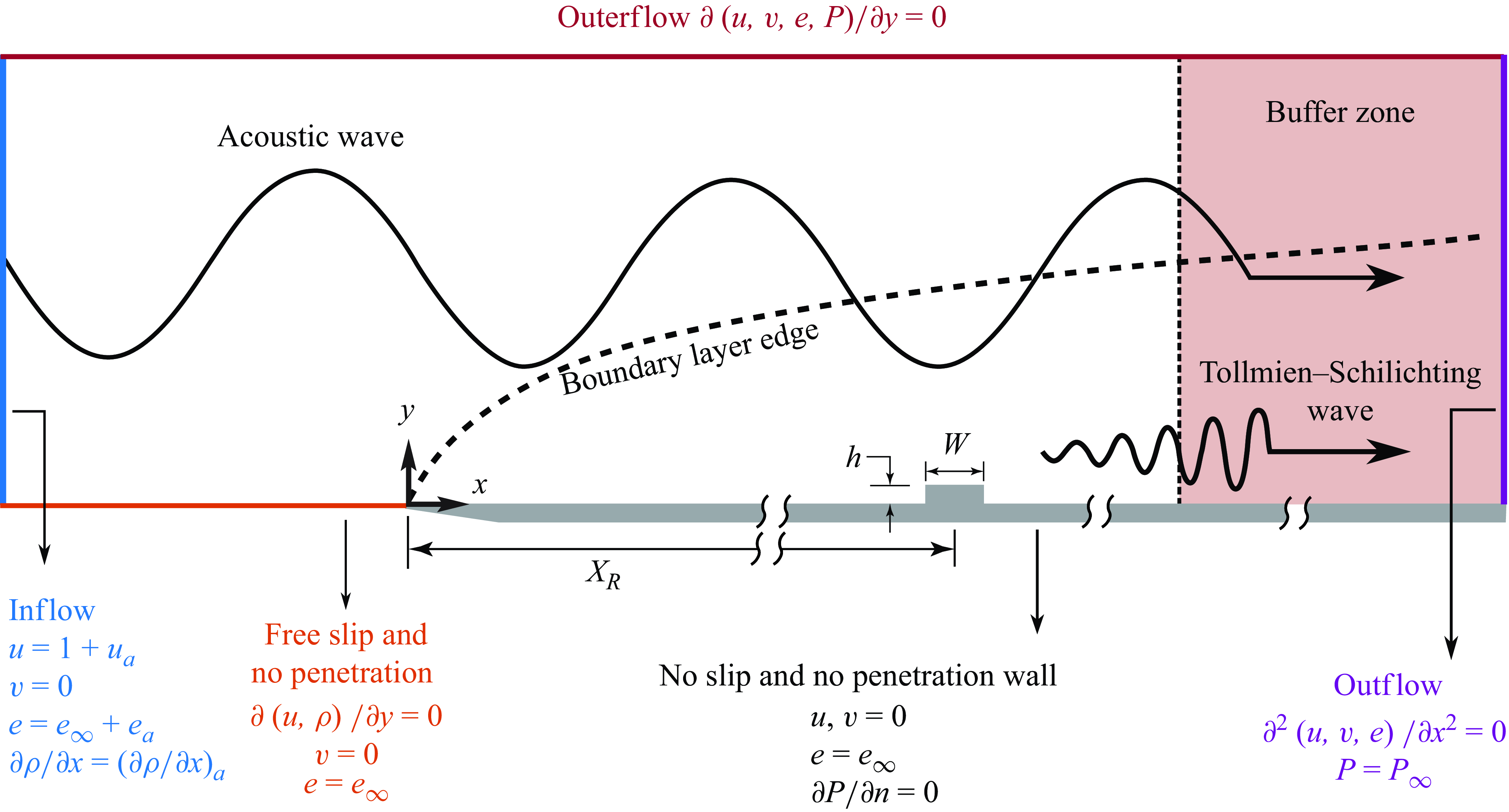
Scheme of the simulation set-up with boundary conditions and representation of the TS wave resulting from the receptivity at a roughness. Not drawn to scale, but geometrical parameters are indicated.

Figure 1 shows a schematic of the computational domain. It illustrates the acoustic receptivity mechanism with the generation of a TS wave at the bump and indicates the boundary conditions. For obtaining the undisturbed base flow, at the inflow the temperature and the velocities are fixed and uniform and the pressure gradient in the streamwise direction is set to zero. Along the wall, the no-slip and no-penetration conditions are imposed. The temperature is fixed and the pressure gradient is set to null along the wall-normal direction (Bergamo et al. Reference Bergamo, Gennaro, Theofilis and Medeiros2015). Upstream of the plate a free-slip region is used towards accommodating the flow upstream of the plate leading edge and controlling the pressure variations associated with the stagnation point (Mathias & Medeiros Reference Mathias and Medeiros2018, 2021). The outer boundary is subject to a homogeneous Neumann boundary condition along the y direction for all variables. The second-order derivatives along the x direction of all variables are set to zero at the outflow, except for the pressure, which is prescribed. The boundary conditions for pressure are transported to density using the ideal-gas relations. The buffer zone length is adjusted to damp the acoustic wave by a factor of at least
 $10^{3}$
.
At the corner nodes, the pressure is determined by averaging the values that satisfy the Neumann condition for the pressure gradient in each direction. This averaging has virtually no influence on the results as both values come very close to each other. Using either value leads to essentially the same solution, but we employ the mean to avoid bias. At the corners, we used effectively identical grid spacing in both
 $Y$
and
 $X$
directions to further minimise possible bias. Although the method is strictly a lower-order approximation, it does not appreciably affect the solution accuracy (Silva et al. Reference Silva, Souza and Medeiros2009). The mesh convergence tests showed it does not compromise the quality of the solution.
After the base flow is obtained, the inflow boundary conditions follow the conditions prescribed in § 2.3. Note that the simulations are performed for an acoustic wave propagating parallel to the wall, and hence reflection of sound on the plate does not occur. This is a special case of acoustic wave propagation. For a compressible boundary layer with O(1) Mach number, the incident sound wave would in general propagate at an arbitrary direction with respect to the wall so that reflections by the wall take place. This general case is investigated in Dong et al. (Reference Dong, Liu and Wu2020) and Liu et al. (Reference Liu, Dong and Wu2020), where simulations of receptivity due to a sound wave interacting with a smooth bump were performed for a general incidence angle.
The flow parameters involved are: Reynolds number (
 ${\textit {Re}}_{\delta ^*_b} = U_{\infty }^*\delta ^*_b/\nu ^*_\infty$
); Mach number (
 $M\!a$
); non-dimensional frequency (
 $F = (2\pi f^* \nu ^*_\infty )/U^{*2}_\infty$
). In these definitions,
 $U^*_\infty$
is the free stream velocity,
 $\delta ^*_b$
is the undisturbed Blasius displacement thickness at a position corresponding to the leading edge of the bump/gap,
 $\nu ^*_\infty$
is the free stream kinematic viscosity and
 $f^*$
is the acoustic wave frequency. Except when explicitly indicated otherwise, the present numerical simulations were conducted at
 ${\textit {Re}}_{\delta ^*_b} = 1413.8$
and
 $F \times 10^6 = 25.85$
, the same as in Placidi et al. (Reference Placidi, Gaster and Atkin2020). The Mach number was
 $M\!a = 0.1$
and the free stream acoustic wave amplitude
 $A_a = 3.16 \times 10^{-5}$
. All the lengths were normalised by
 $\delta ^*_b$
. The bump heights (or gap depths),
 $h$
, varied within
 $ [0.042 , 0.336]$
. The physical domain was
 $X = [-100 , 1200]$
and
 $Y = [0, 38]$
. The bump/gap leading edge was positioned at
 $X = 478.8$
and their width was
 $W=16.8$
. The maximum receptivity occurs when the bump width is half the wavelength of the excited TS wave Goldstein (Reference Goldstein1985). According to Placidi et al. (Reference Placidi, Gaster and Atkin2020), for the frequency chosen, this width would correspond to
 $W=23.52$
(28 mm in their experimental rig). For practical reasons, they utilised a 20 mm wide bump (
 $W=16.8$
), and they estimated a reduction of approximately 10 % in the magnitude of the resulting TS wave.
2.3. Flow perturbations
To introduce the acoustic wave, the following harmonic perturbation matching the free stream acoustic impedance (which gives a relationship among velocity, energy and pressure) was superimposed to the inflow boundary condition:
 \begin{align} u_{a} = \, A_a \, \exp (\omega t),\qquad\qquad \end{align}
 \begin{align} e_{a} = \, A_a \,\frac {c_{a}-1}{\gamma }\exp (\omega t),\quad\qquad\end{align}
 \begin{align} \left ( \frac {\partial \rho }{\partial x} \right )_a = \, \frac {(c_{a}-1) \, \partial u_{a} / \partial x \, - \, \rho \, \partial e / \partial x}{e (\gamma -1)} ,\end{align}
where
 $\gamma$
is the specific heat ratio,
 $\omega = 2\pi f$
,
 $c_a = 1 + 1/M\!a$
is the acoustic wave propagation velocity relative to the wall and
 $A_a$
is the amplitude of the acoustic wave.
Equations (2.1) to (2.3) were based on the impedance relations derived from the inviscid acoustic wave solution (i.e. an acoustic wave propagating in the free stream far from the wall) which is available in Raposo et al. (Reference Raposo, Mughal and Ashworth2019), and were consistent with a Dirichlet boundary condition for velocity and energy and a Neumann boundary condition for pressure.
As will be explained in § 3.1, simulations of a TS wave without the acoustic wave were required for estimating the equivalent initial amplitude of the TS wave resulting from the receptivity (
 $TS_{rc}$
) at the roughness position. These were simulations of TS waves on a smooth plate (
 $TS_{sm}$
) and on the rough plate (
 $TS_{rg}$
). These simulations used the same high-fidelity code. To ensure a well-developed TS wave over the bump/gap position, the
 $TS_{sm}$
and
 $TS_{rg}$
were introduced by localised suction and blowing on the wall centred at
 $X\approx 337$
which is more than two TS wavelengths upstream of the roughness. The suction and blowing were applied over a length roughly corresponding to one TS wavelength.
3. Preliminary results
3.1. Receptivity process and its quantification
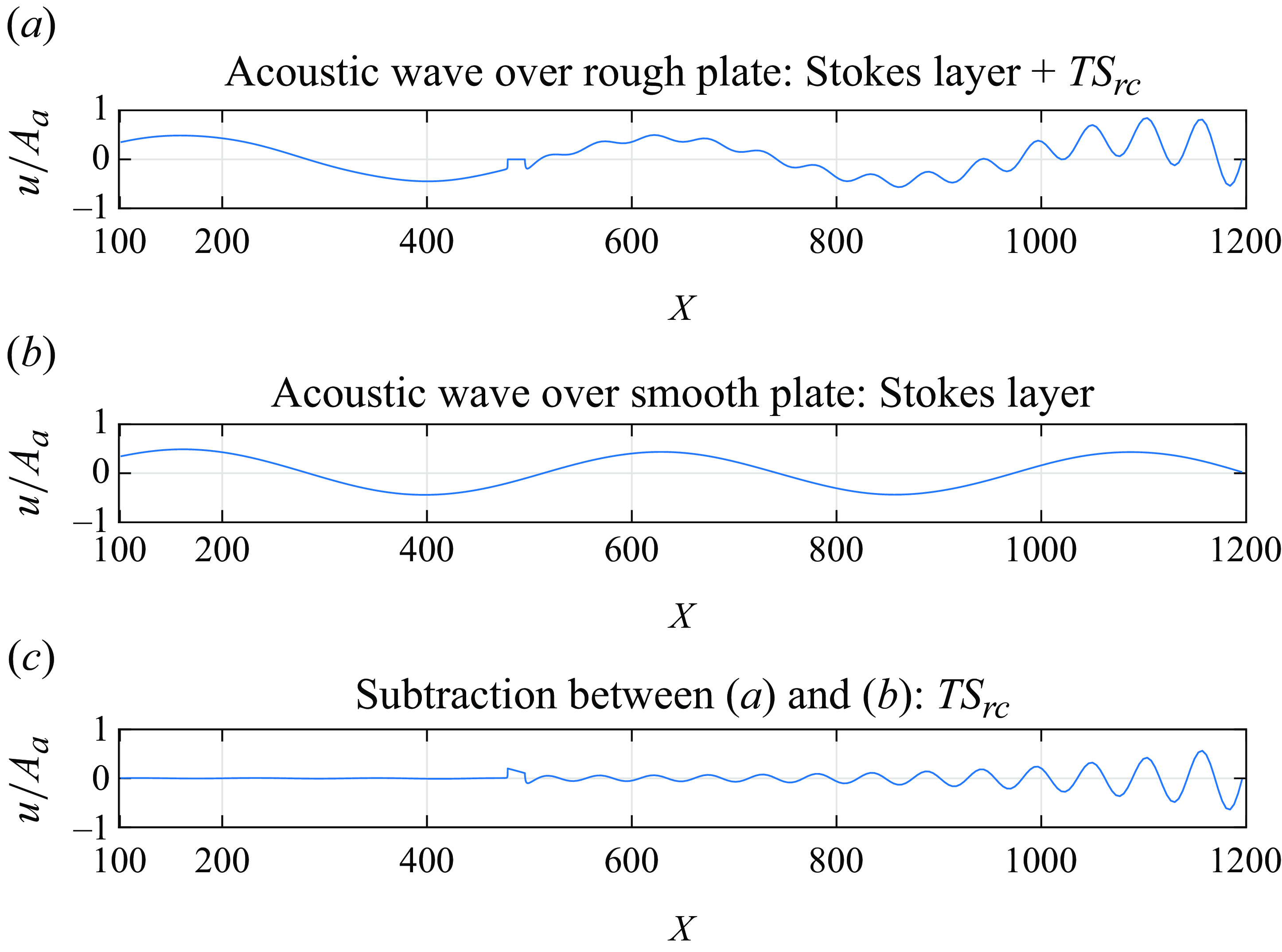
Snapshots of streamwise velocity disturbances at
 $y=12.6$
associated with an acoustic wave. The velocity is normalised by the free stream acoustic wave amplitude (
 $A_{a}$
). Surface with a bump (a) and smooth plate (b). Panel (c) is the difference between the disturbances fields (a) and (b). Here
 $TS_{rc}$
is the TS wave inserted by the acoustic receptivity at the roughness. The results correspond to a bump with
 $h=12.6\,\%$
,
 ${\textit {Re}}_{\delta ^*_b} = 1414$
and
 $M\!a = 0.3$
.

Figure 2(a) shows
 $TS_{rc}$
in combination with the corresponding acoustic wave. As the
 $TS_{rc}$
has the frequency of the acoustic wave, extracting it from the flow is not trivial. Different strategies have been used in previous studies available in the literature (Würz et al. Reference Würz, Herr, Wörner, Rist, Wagner and Kachanov2003; Monschke et al. Reference Monschke, Kuester and White2016; Placidi et al. Reference Placidi, Gaster and Atkin2020). Here the subtraction procedure proposed by Placidi et al. (Reference Placidi, Gaster and Atkin2020) was employed. It requires a simulation of an identical acoustic wave over a plate without the bump, figure 2(b). Next, we subtract figure 2(b) from figure 2(a) and obtain the
 $TS_{rc}$
shown in figure 2(c).
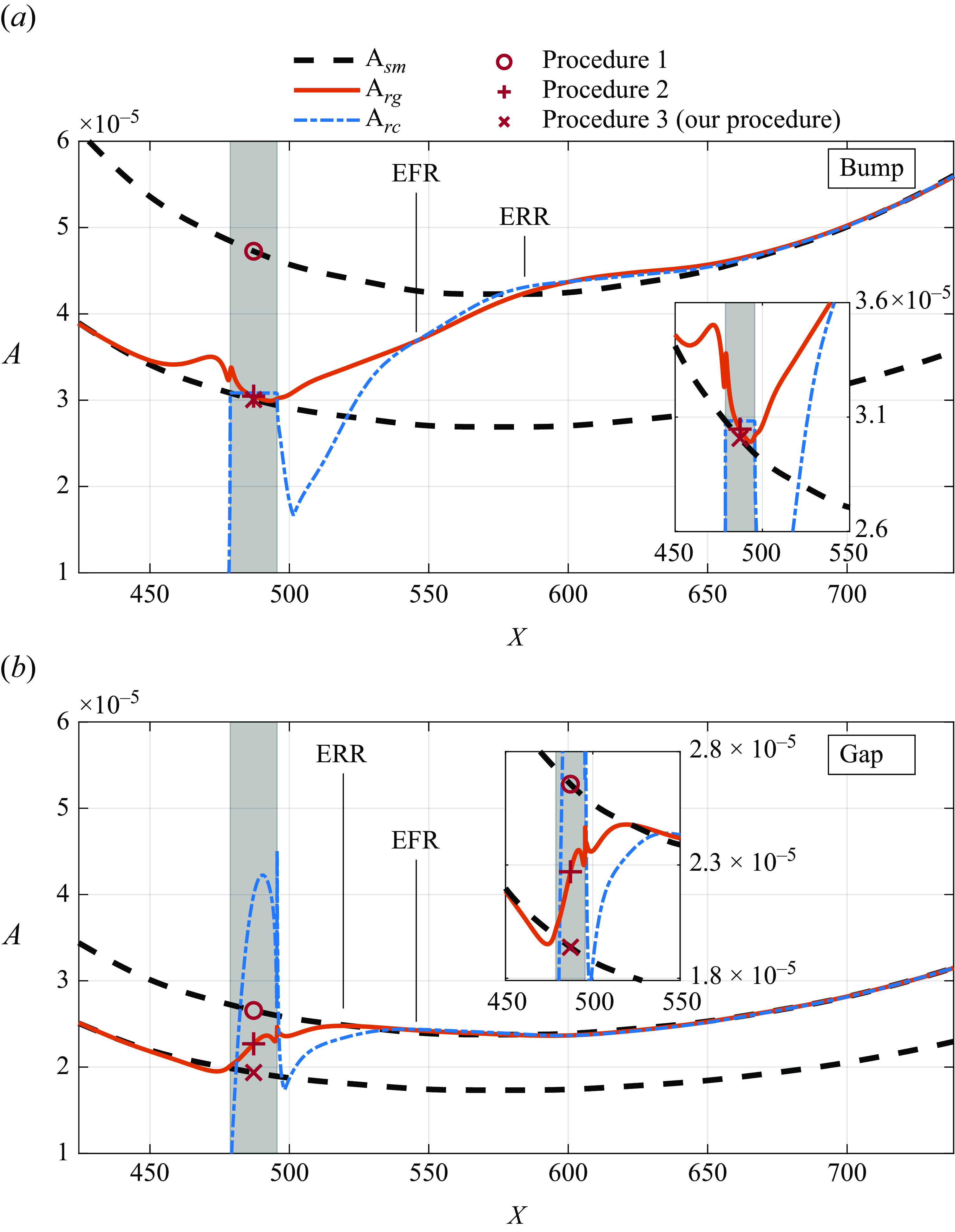
Evolution of the maximum amplitude of
 $TS_{sm}$
(dashed black),
 $TS_{rg}$
(solid red) and
 $TS_{rc}$
(dashed–dotted blue). Markers represent different estimates of the receptivity amplitude: procedure 1 (
 $\circ$
); procedure 2 (
 ${+}$
); procedure 3 (
 $\times$
). Results correspond to
 $|h| = 33.6\,\%$
. The grey rectangle indicates the roughness element position. Panel (a) for the bump and (b) for the gap. The insert shows zoomed-in views of parts of the figures.

It is important to note that, in principle, there is also the receptivity from the interaction of the acoustic wave with the leading edge (Goldstein Reference Goldstein1983; Ruban Reference Ruban1984; Goldstein Reference Goldstein1985; Heinrich & Kerschen Reference Heinrich and Kerschen1989; Choudhari & Streett Reference Choudhari and Streett1992). This interaction is present both in the simulation with and without the bump (figures 2 a and 2 b, respectively), hence it is also removed by the procedure. For the simulation with the bump (figure 2 a) there would still be an amplification effect due to the bump on the TS wave generated at the leading edge. For the small bumps considered, this would lead to only a small amplification of the oncoming TS wave. Moreover, the TS wave generated at the leading edge also tends to be small owing to the decay prior to the lower branch of the stability loop (Goldstein Reference Goldstein1983). In our study, we did not find any indication of contamination from a TS wave generated at the leading edge. This contamination would appear as an oscillation with a different wavelength (the TS wavelength) superposed to the Stokes layer that is formed by the acoustic wave (Ruban Reference Ruban1984; Goldstein Reference Goldstein1985; Choudhari & Streett Reference Choudhari and Streett1992). In our simulations, some distance upstream of the roughness the flow oscillations conformed to a Stokes layer, without any indication of contamination of the type described above, figure 2(b).
Besides extracting the TS wave from the flow, there are other issues involved in estimating the receptivity equivalent initial amplitude. These issues are illustrated in figure 3 for
 $h = \pm 33.6\,\%$
. The
 $TS_{rc}$
is the main curve of interest, but the plots show three other auxiliary curves and a grey area that indicates the roughness element position. All curves are in a regime where they scale linearly with the TS amplitude (see appendix A.1), hence their growth rate does not depend on their amplitude. The dashed black line and the red line represent reference linear evolution of a TS waves and serve to identify the different stages undergone by the
 $TS_{rc}$
, as will be explained. The dashed black lines represent the evolution of a TS wave on smooth surface,
 $TS_{sm}$
. The vertical position (that is, the position on the yaxis of the figure) of the higher dashed line is chosen to match the
 $TS_{rc}$
far downstream, where
 $TS_{rc}$
behaves as a
 $TS_{sm}$
. The red curve represents a TS wave generated well upstream of the roughness and evolving on a surface with a roughness element
 $TS_{rg}$
. Its vertical position was also chosen to match
 $TS_{rc}$
far downstream. The vertical position of the lower black dashed line is chosen to match the
 $TS_{rg}$
far upstream, where
 $TS_{rg}$
behaves as a
 $TS_{sm}$
.
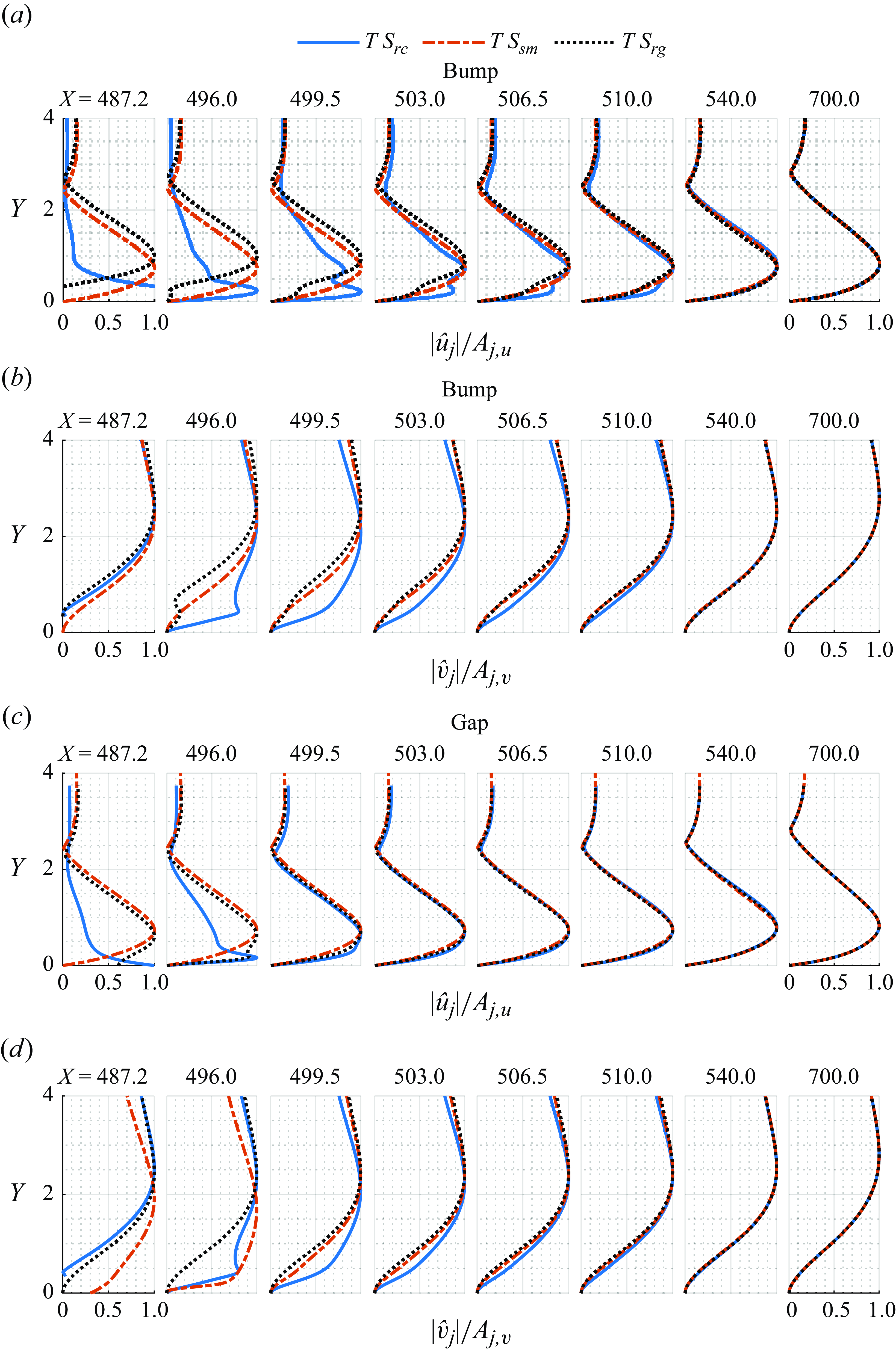
Disturbance velocity profiles for
 $TS_{rc}$
,
 $TS_{rg}$
and
 $TS_{sm}$
at different stations, normalised by their local maxima. The results correspond to the bump and the gap with
 $|h|= 33.6\,\%$
: (a) and (b) for the bump; (c) and (d) for the gap; (a) and (c) streamwise velocity; (b) and (d) wall-normal velocity.

We divide the evolution of the
 $TS_{rc}$
into three stages. The first we called formation region whose end is marked EFR (end of formation region). The second is called recovery region (Klebanoff & Tidstrom Reference Klebanoff and Tidstrom1972), and its end is marked ERR (end of recovery region). After the recovery region, the TS wave evolves according to the smooth plate behaviour which is the third part of the evolution. Looking first at the bump case, in the formation region the
 $TS_{rc}$
experiences a sharp decay and a large growth. In this region, the TS wave is not yet fully formed. This behaviour is best shown by figure 4 that displays the normalised profiles of the velocity fluctuations, for the
 $TS_{rc}$
,
 $TS_{rg}$
and
 $TS_{sm}$
. In this figure,
 $\hat {u}_{j} = \mathcal {F}({u}_{j})$
is the Fourier transform in time of the streamwise velocity disturbance, where ‘
 $j$
’ stands for wave over smooth plate ‘sm’, wave over rough plate ‘rg’ and receptivity wave ‘rc’. Similar definition applies to
 $\hat {v}_{j}$
. Note that only for
 $TS_{sm}$
and
 $TS_{rg}$
the TS wave disturbance was excited by suction and blowing condition upstream of the roughness location (see § 2.3). Close to the bump the
 $TS_{rc}$
profiles do not conform to the TS wave ones. They are very distorted and display different velocity peaks. It is only at approximately
 $X = 540$
, EFR, that the
 $TS_{rc}$
profile becomes similar to that of the
 $TS_{sm}$
and
 $TS_{rg}$
. Perhaps in the formation region the
 $TS_{rc}$
fluctuations cannot yet be called TS waves (Wu Reference Wu2001). There the fluctuations are non-modal. In any case, we still refer to them as TS waves and even discuss their growth rates. However, the concept of growth rate in this region is rather loose.
After EFR, the
 $TS_{rc}$
closely follows the
 $TS_{rg}$
. In this region, the TS wave evolves towards the smooth plate regime farther downstream. In the recovery region of the bump the
 $TS_{rg}$
experiences a much larger growth than that on a smooth plate. We prefer to place the ERR at approximately
 $X=580$
and disregard the small overshooting that exists there. The recovery region concept was defined in the context of a pre-existing TS wave that interacts with a bump and eventually returns to its flat plate growth rate downstream. Here there is no
 $TS_{rc}$
upstream of the bump, hence the word recover is perhaps not entirely appropriate. Nevertheless in these regions, the base flow profiles also return to the smooth plate ones, and for that reason, we preferred to maintain the same nomenclature. It must also be observed that the formation region is embedded into the recovery region because there the base flow profiles are distorted by the bump. After the recovery region, the TS wave assumes its smooth plate regime, the third part of the evolution. In summary, for the bump, there is a region where the TS wave is not formed and is under the influence of the bump; an intermediary region where the TS wave is already formed but evolves under the influence of the bump; and then the smooth plate regime.
Next, looking into the gap case, figure 3 shows some important differences and similarities with respect to the bump case. As explained is § 3.1, the formation region ends where the
 $TS_{rc}$
(blue dashed–dotted line) reaches the
 $TS_{rg}$
(red solid line) and the recovery region ends where the
 $TS_{rg}$
reaches the
 $TS_{sm}$
(higher dashed black line). Figure 3 shows that, as opposed to the bump, for the gap the recovery region ends at
 $X \approx 520$
, upstream of the end of the formation region (at
 $X \approx 546$
). The figure also indicates that the formation region ends at approximately the same station for both bumps and gaps. The inversion occurs because of a variation in the extent of the recovery region, not the formation region. The extent of the formation region is further explored in § 4.
Another issue addressed in figure 3 is the estimate of the outcome of the receptivity process. These constitute the procedures 1 and 2 addressed in the introduction. They use some kind of extrapolation to estimate the so-called equivalent initial amplitude, which is obtained at the roughness centre. They do not involve any backwards or upstream integration. The extrapolations are based on the linear evolution of TS waves presented as black dashed and red solid lines in figure 3. We also propose another procedure, named procedure 3. These procedures are summarised as follows.
-
(i) For procedure 1, the upstream extrapolation is based on a smooth plate TS evolution and is represented by the upper dashed black line in figure 3. Its equivalent initial amplitude at the bump centre indicated by the circle in figure 3.
-
(ii) For procedure 2, the upstream extrapolation is based on a TS wave evolution on a plate with a roughness element, red line in figure 3. Its equivalent initial amplitude at the bump centre indicated by the symbol + in figure 3.
-
(iii) For procedure 3, the upstream extrapolation is based on the evolution of a TS wave evolving on a plate with a roughness element (red line in figure 3) and is followed by a downstream extrapolation based on the smooth plate TS wave evolution (lower dashed black line in figure 3). The rationale behind this procedure is explained below. Its equivalent initial amplitude at the bump centre indicated by the cross symbol in figure 3.
Owing to strong non-parallel effects, procedure 2 does not provide an oscillation that, at the roughness, is modal. As seen in figure 4 the profiles of the
 $TS_{rg}$
at the roughness position are very distorted and do not resemble a
 $TS_{sm}$
profiles. The definition of a TS amplitude (whether maximum
 $u$
, maximum
 $v$
, energy, etc.) would substantially affect the estimates. Moreover, the fluctuation amplitudes vary substantially along the roughness length, particularly for the gap (figure 3
b). The equivalent initial TS wave amplitude would vary substantially depending on the X position where it is evaluated.
To circumvent these shortcomings we proposed procedure 3. This procedure involves the use of another
 $TS_{sm}$
evolution represented by the lower dashed black line in figure 3. The vertical position of this line is matched to the
 $TS_{rg}$
well upstream where the roughness has not yet affected the
 $TS_{rg}$
. This procedure provides a well-defined TS wave at the roughness centre from which an equivalent initial amplitude can be unequivocally obtained.
For the bump, the result is very close to that of procedure 2, but for the gaps, the results are substantially different. The effect of a roughness element on pre-existing TS waves can be quantified by the transmission coefficient proposed by Wu & Hogg (Reference Wu and Hogg2006), Wu & Dong (Reference Wu and Dong2016) and Xu et al. (Reference Xu, Sherwin, Hall and Wu2016). This transmission coefficient is the ratio between the circle and the cross, in which the bump and gap considered (
 $h = \pm 33.6\,\%$
) are approximately 1.6 and 1.4, respectively. So, procedure 3 is consistent with the receptivity theories that do not account for the amplification effect and is also consistent with the transmission coefficient concept. The outcome of the combined processes is given by the product of the equivalent initial amplitude and the transmission coefficient.
In this paper, we present results based on the three procedures. It will be seen that, in comparison with procedure 1, procedures 2 and 3 agree better with the theoretical predictions of the triple deck type. This agreement is expected because these theories do not account for the effect of the roughness on the TS wave evolution, the amplification effect. It will also be seen that procedures 2 and 3 lead to different trends for the effect of gap depth on receptivity.
Another way to measure receptivity is via the efficiency function for the streamwise velocity,
 \begin{equation} |\Lambda _u| = \frac {A_0}{A_a\,|h|\,|\mathcal {H}|(\alpha _{TS})}, \end{equation}
where
 $A_0$
is the receptivity equivalent initial amplitude. Here
 $\mathcal {H} = \mathcal {F}(S_{rg})$
is the space domain Fourier transform of
 $S_{rg}$
, which is the shape of the roughness normalised by its height/depth. Here
 $\mathcal {H}(\alpha _{TS})$
is evaluated at the complex wavenumber
 $\alpha _{TS}$
of
 $TS_{sm}$
at the roughness element centre (
 $X_R$
). Recall that
 $A_{a}$
is the free stream acoustic wave amplitude and
 $h$
is the height/depth of the roughness element.
3.2. Comparison with other numerical results
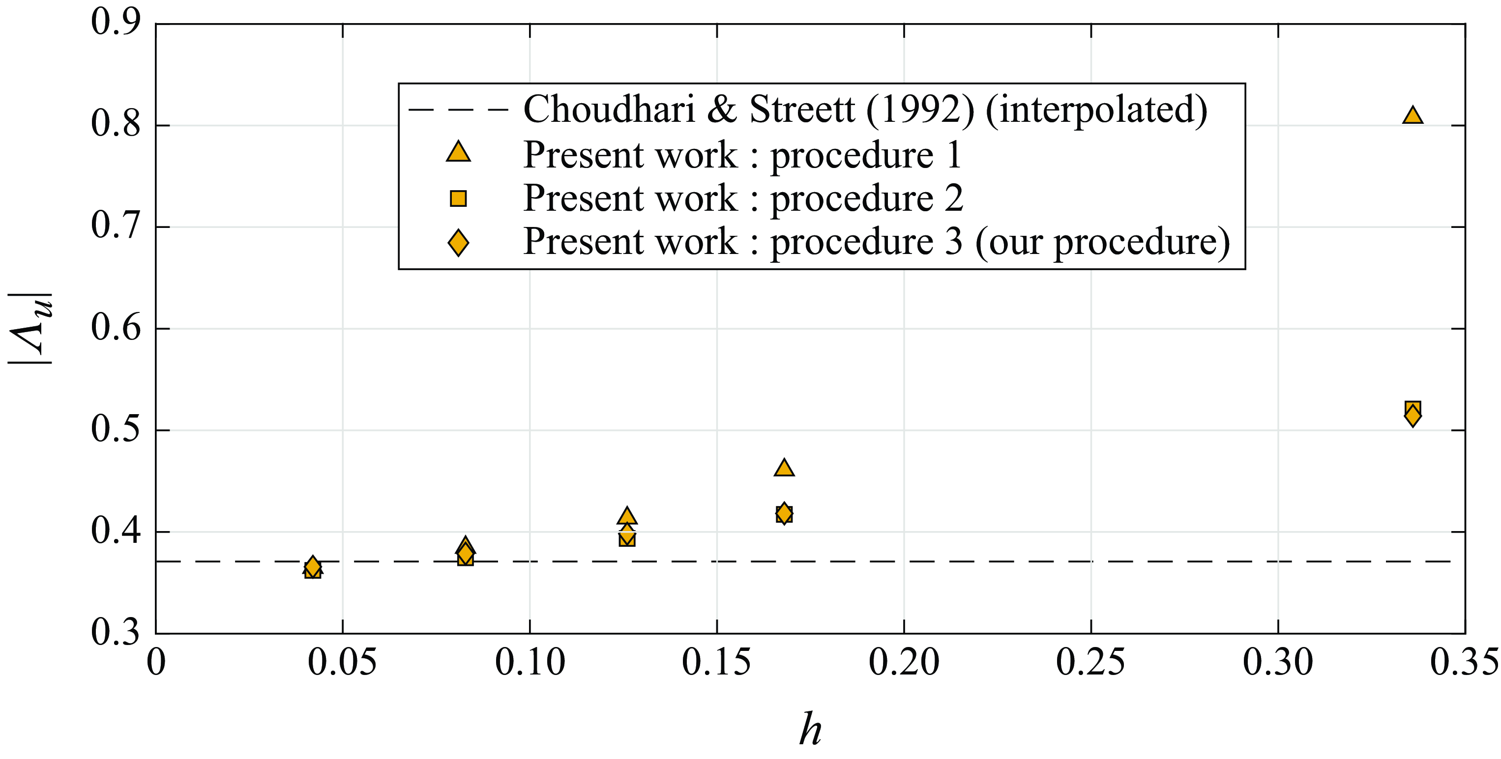
Figure 5 compares the results from Choudhari & Streett (Reference Choudhari and Streett1992) and the present work using procedures 1, 2 and ours. For
 $h= 5\%$
the procedures are equivalent. For
 $h=12.6\,\%$
procedure 1 departs substantially from procedures 2 and 3 which remain fairly close. Results also indicate that at 12.6 % for all procedures the linear theory underpredicts the results. We anticipate that for gaps such comparison leads to different conclusions.
Comparison of efficiency function obtained with different procedures. The Choudhari & Streett (Reference Choudhari and Streett1992) data was interpolated to
 ${\textit {Re}}_{\delta ^*_b} = 1413.8$
.

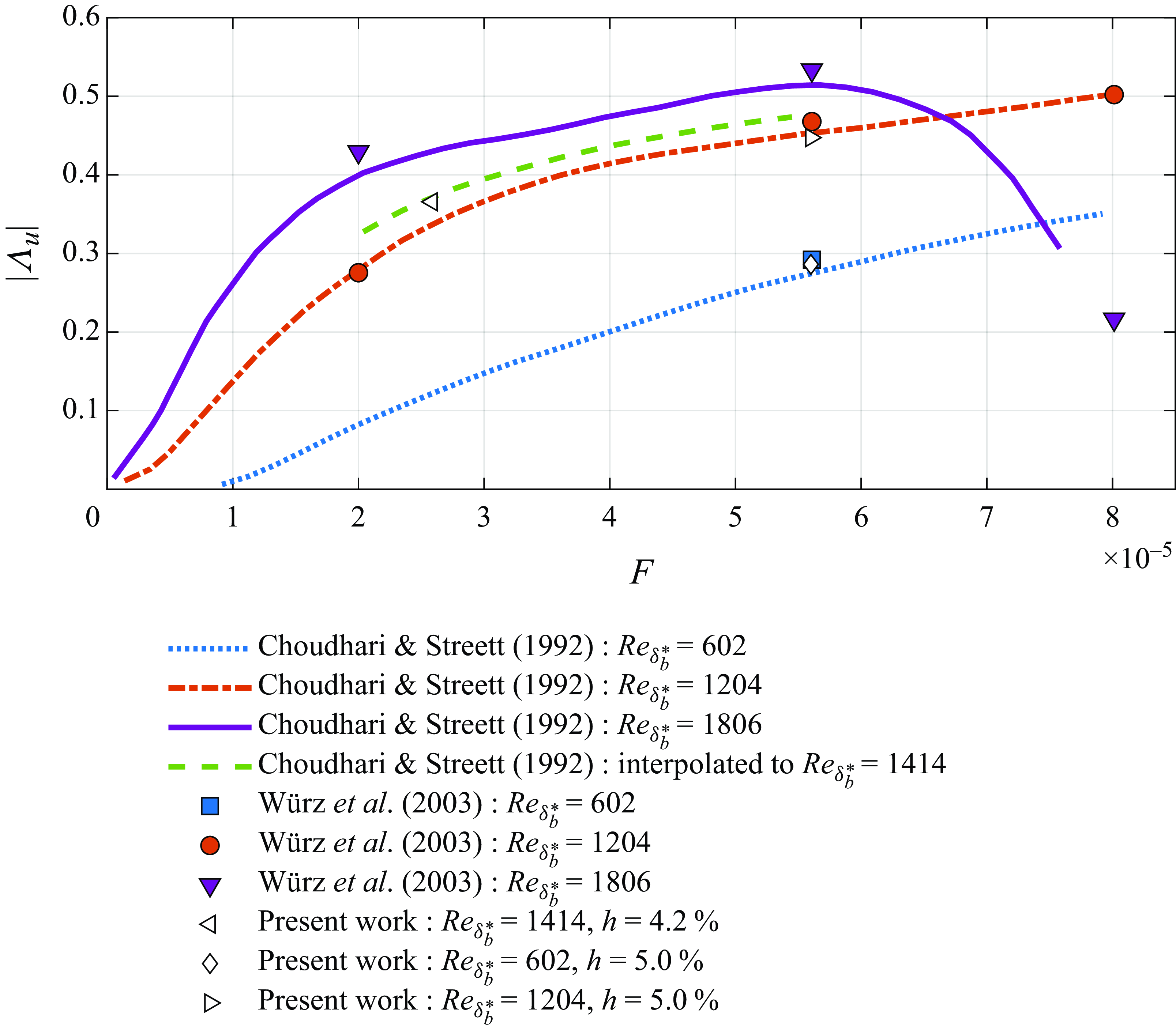
Figure 6 shows a comparison of the present results with the numerical results from Würz et al. (Reference Würz, Herr, Wörner, Rist, Wagner and Kachanov2003) and the FRNT of Choudhari & Streett (Reference Choudhari and Streett1992). Overall, there was good agreement among the three approaches.
Comparison of the theoretical results from Choudhari & Streett (Reference Choudhari and Streett1992) with results from Würz et al. (Reference Würz, Herr, Wörner, Rist, Wagner and Kachanov2003) (using procedure 2) and the current DNS results (using our procedure).

3.3. Comparison with experimental results
Simulations were also conducted for the experimental conditions from Placidi et al. (Reference Placidi, Gaster and Atkin2020). Here the
 $M\!a$
was set to
 $0.1$
which, as discussed in appendix A.2, is low enough to represent the incompressible conditions of the flow while avoiding the use of the code at yet lower
 $M\!a$
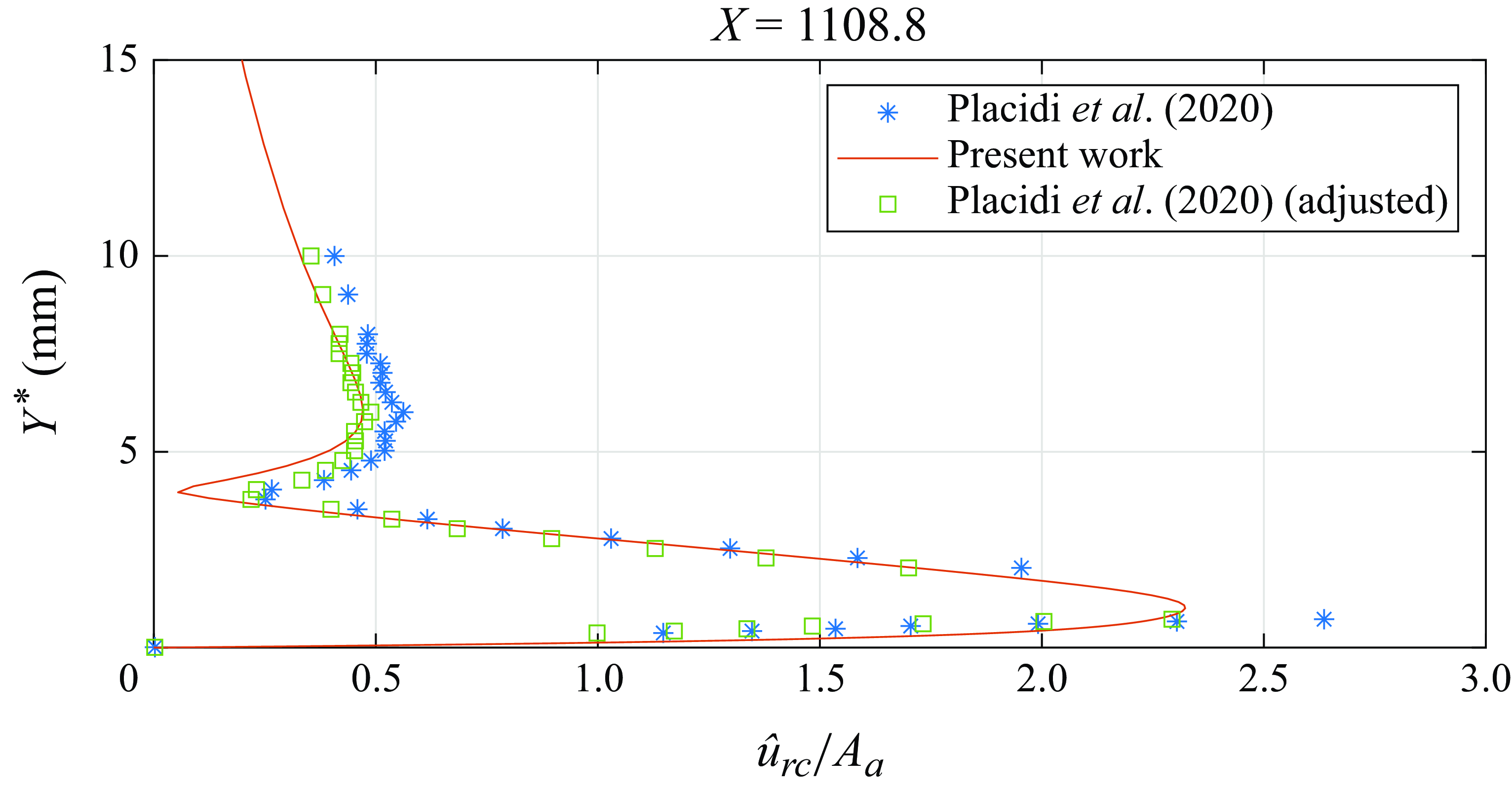
conditions, which is inefficient. Figure 7 compares the experimental (figure 4b in Placidi et al. Reference Placidi, Gaster and Atkin2020) and numerical TS wave profiles at a position (
 $X = 1108.8$
) far downstream from the bump. Despite showing similar shapes, the amplitude of the TS wave from the simulation was smaller than that of the experiment. However, if we multiply the experimental data by a single scaling factor of 0.87, the agreement is excellent.
Comparison of the
 $TS_{rc}$
amplitude profile (
 $\hat {u}_{TS}$
) normalised by
 $A_{a}$
from the present DNS with the experimental results from Placidi et al. (Reference Placidi, Gaster and Atkin2020), and the experimental results adjusted by a single factor. Bump height
 $h=12.6\,\%$
.

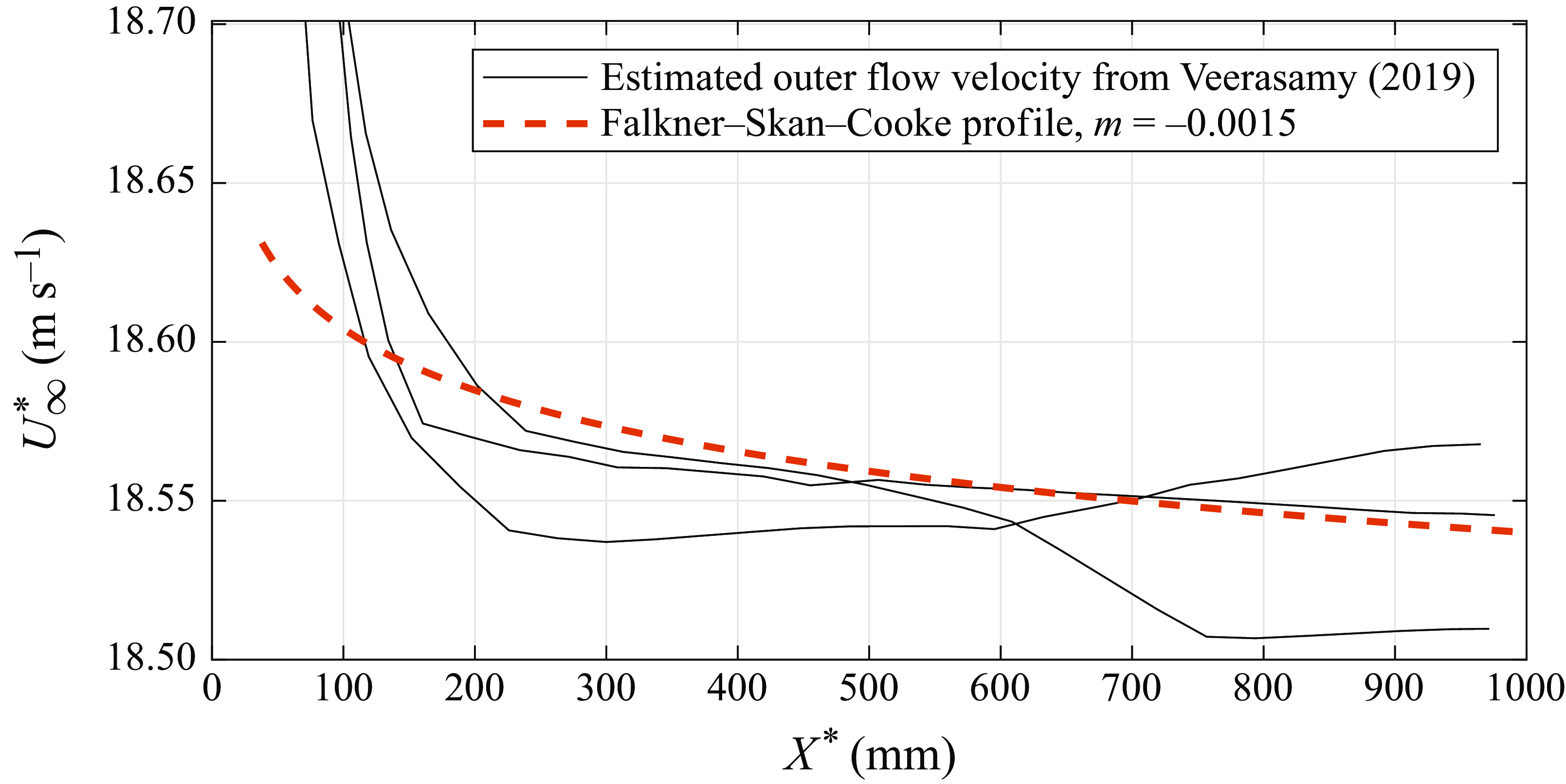
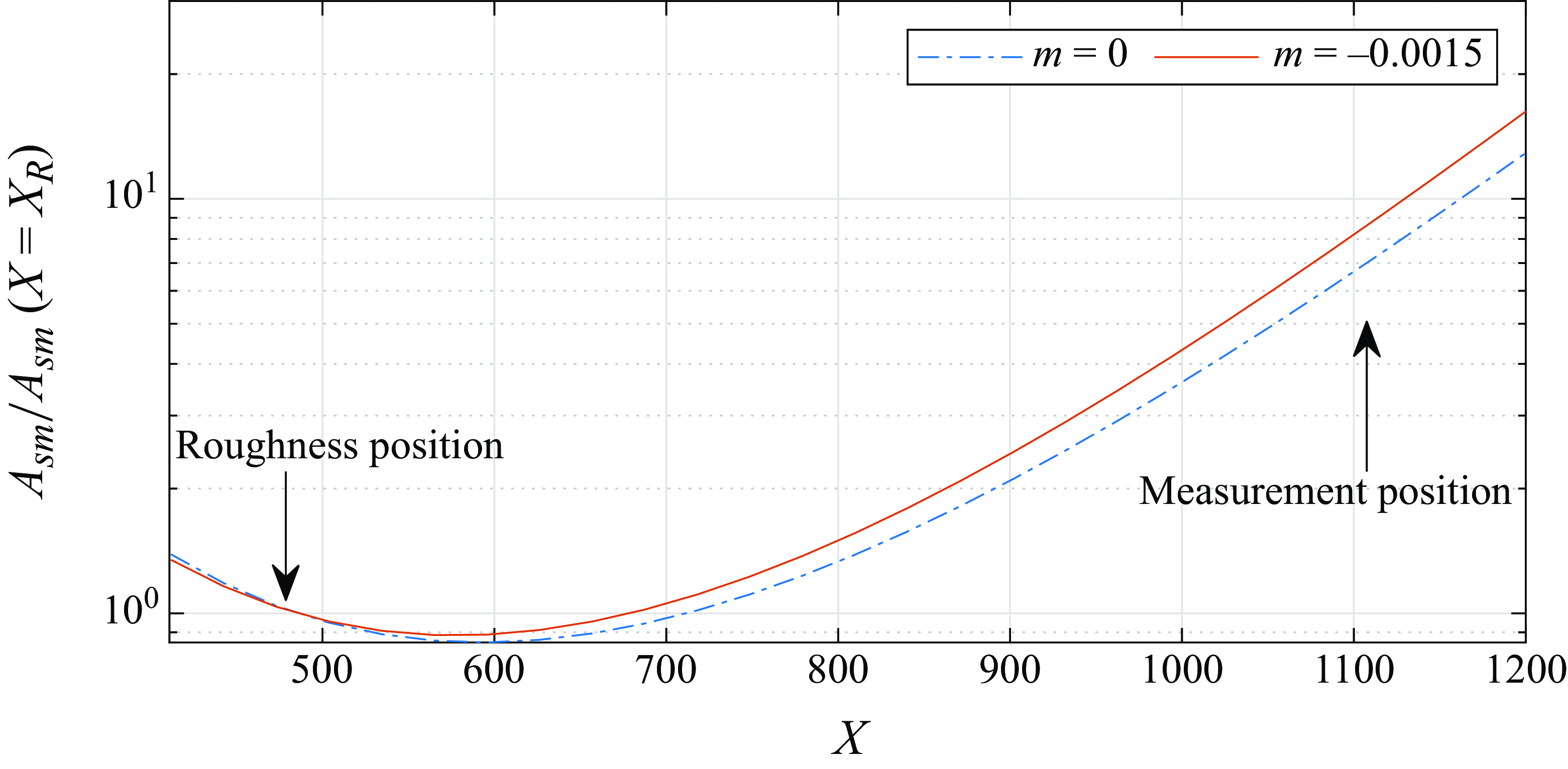
The effect of the bump on the downstream evolution of the TS wave cannot explain the discrepancy as both estimates incorporate the same effect. However, the pressure gradient in the experiment is never perfectly null. In figure 8 we present the free stream velocity distributions given by Veerasamy (Reference Veerasamy2019), which is reported by Placidi et al. (Reference Placidi, Gaster and Atkin2020) as representative of a typical situation in their wind tunnel. Figure 9 compares the evolution of the TS wave with and without the estimated pressure gradient. The influence of a mild pressure gradient corresponding to
 $m = -0.0015$
(
 $m$
being the parameter in Falkner–Skan–Cooke model) is sufficient to cause approximately
 $30\,\%$
increase in the TS wave amplitude at the measuring station. This increasing could potentially explain the disagreement between numerical and experimental results. This issue is further addressed in the next section.
Streamwise velocity variation: solid lines, typical free stream velocity distributions over the plate in the experiment, as reported by Placidi et al. (Reference Placidi, Gaster and Atkin2020); dashed lines, Falkner–Skan–Cooke free stream velocity distribution for
 $m = -0.0015$
.

The TS wave evolution calculated with a parabolised stability equation (PSE) code over a flat plate with zero pressure gradient and with
 $m=-0.0015$
.

4. Acoustic receptivity of bumps and gaps
4.1. Base flow
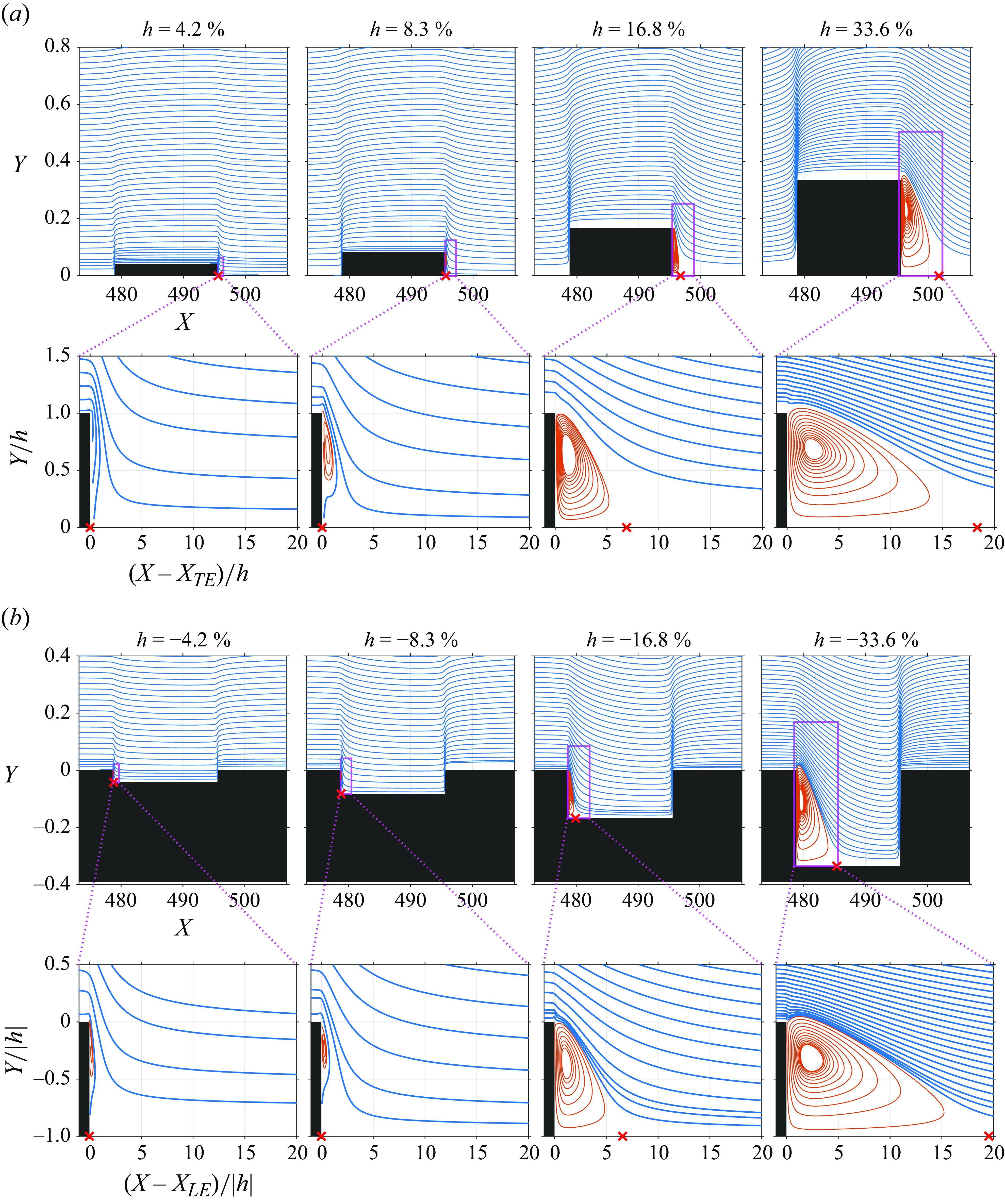
The streamlines of the base flows for bumps with width
 $W=16.8$
and different heights are presented in figure 10(a). At
 $h=4.2\,\%$
, no recirculating bubble is noticeable in the plot scale. At
 $h=8.3\,\%$
, a recirculating bubble is seen aft of the trailing edge of the bump (
 $X_{TE}$
). However, even up to
 $h = 12.6\,\%$
the recirculating bubbles is still much shorter than a TS wavelength. At
 $h = 33.6\,\%$
the bubble length is much longer.
Streamlines for cases with roughness of different heights: (a) bumps and (b) gaps. The red streamlines indicate the recirculating flow region that reattaches on the plate at the location marked with red symbols. Here
 $X_{LE}$
and
 $X_{TE}$
denote the element’s leading edge and trailing edge location, respectively. In all cases,
 $M\!a = 0.1$
, the elements are centred at
 ${\textit {Re}}_{\delta ^*_b} = 1414$
and have
 $W=16.8$
.

Figure 10(b) presents the streamlines of the base flows of gaps. The flow in the vicinity of the leading edge of the gap is very similar to that of the trailing edge of the bump. Up to
 $h=-8.3\,\%$
, almost no recirculating bubble is noticeable in the plot scale, while at
 $h=-12.6\,\%$
, a bubble is observed. Even at h = 16.8 % the bubble length is small. Note that the flow at the gap leading edge is remarkably similar to that of the bump leading edge. For the gap the reattachment point is only slightly farther downstream.
4.2. Receptivity of bumps and gaps
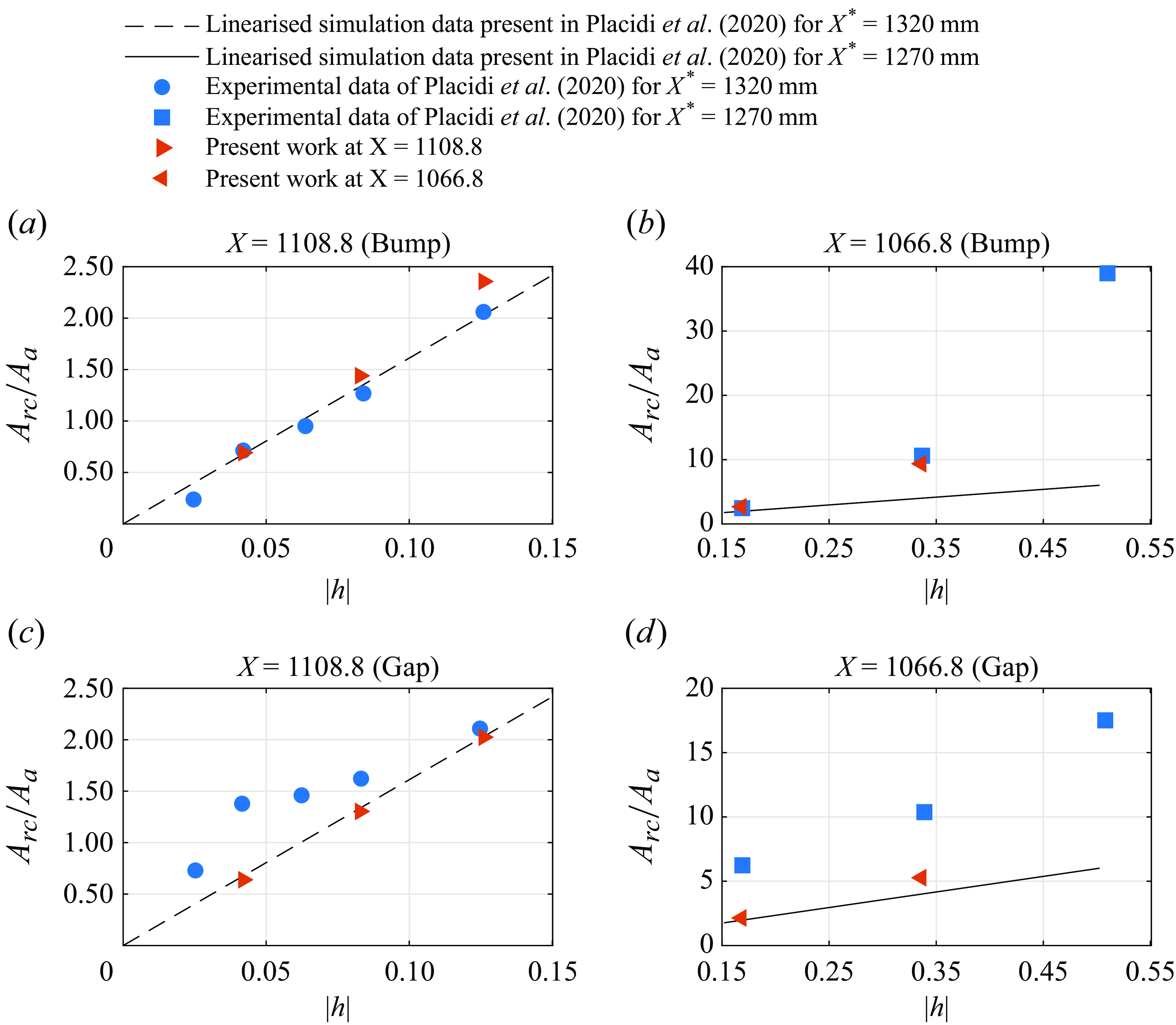
Figure 11 compares experimental results (Placidi et al. Reference Placidi, Gaster and Atkin2020) and our numerical results for the maximum of the
 $TS_{rc}$
at
 $X=1066.8$
or
 $X=1108.8$
, normalised by the free stream acoustic wave amplitude. Those positions correspond to 1270 mm and 1320 mm, which were used in the experiment. The figure also includes the results from linearised simulations presented by Placidi et al. (Reference Placidi, Gaster and Atkin2020). As discussed above, it is possible that the experiment may have had a mild pressure gradient. Hence, to enable a comparison between experiments and simulations a scaling factor was calculated based on the results for the smaller bump,
 $h=4.2\,\%$
. A value of
 $0.7$
was obtained which is consistent with the 30 % amplitude increase associated with a Falkner–Skan–Cooke parameter
 $m=-0.0015$
. With this one-factor correction, all the experimental results were corrected. The agreement between corrected experimental results and simulations for the bumps was good including the regime where the receptivity scales superlinearly with bump heights (figure 11
a,b). This scaling factor of
 $0.7$
is not the same applied in figure 7, which is for the bump with
 $h=12.6\,\%$
. However, this situation is consistent with the mismatch between the experiment and the present DNS results observed in figure 11 for
 $h=12.6$
.
It is reasonable to assume that the bumps and gaps were tested under the same pressure gradient, hence the same factor was applied for the experimental results for gaps. While the experiments show an earlier departure from linear scaling, figure 11(c,d), our numerical results agree fairly well with linear theory up to
 $h=-12.6\,\%$
.
In the literature, the nonlinear scaling of the receptivity with respect to bump height has been referred to as superlinear (Kurz & Kloker Reference Kurz and Kloker2014). For bumps, superlinear scaling has been associated with flow separation (Bodonyi et al. Reference Bodonyi, Tadjfar, Welch and Duck1989). The literature does not cover this aspect for the acoustic receptivity of gaps. In any case, figure 10(b) shows no separation for these small gaps, hence the agreement with linear theory is consistent. Placidi et al. (Reference Placidi, Gaster and Atkin2020) recognised that at such low depths, the experiments were difficult and accuracy could be an issue. These authors suggested (personal communications) that these results would require some confirmation for more definite conclusions.
Here
 $A_{rc}$
introduced by (a,b) bumps and (c,d) gaps obtained some distance from the roughness element, normalised by
 $A_{a}$
. The positions chosen correspond to those from the experiment (Placidi et al. Reference Placidi, Gaster and Atkin2020). The also includes the linearised simulation results reported by Placidi et al. (Reference Placidi, Gaster and Atkin2020) and present high fildely results. Here
 ${\textit {Re}}_{\delta ^*_b} = 1414$
,
 $M\!a = 0.1$
,
 $A_a = 3.16\times 10^{-5}$
and
 $F = 25.85 \times 10^{-6}$
.

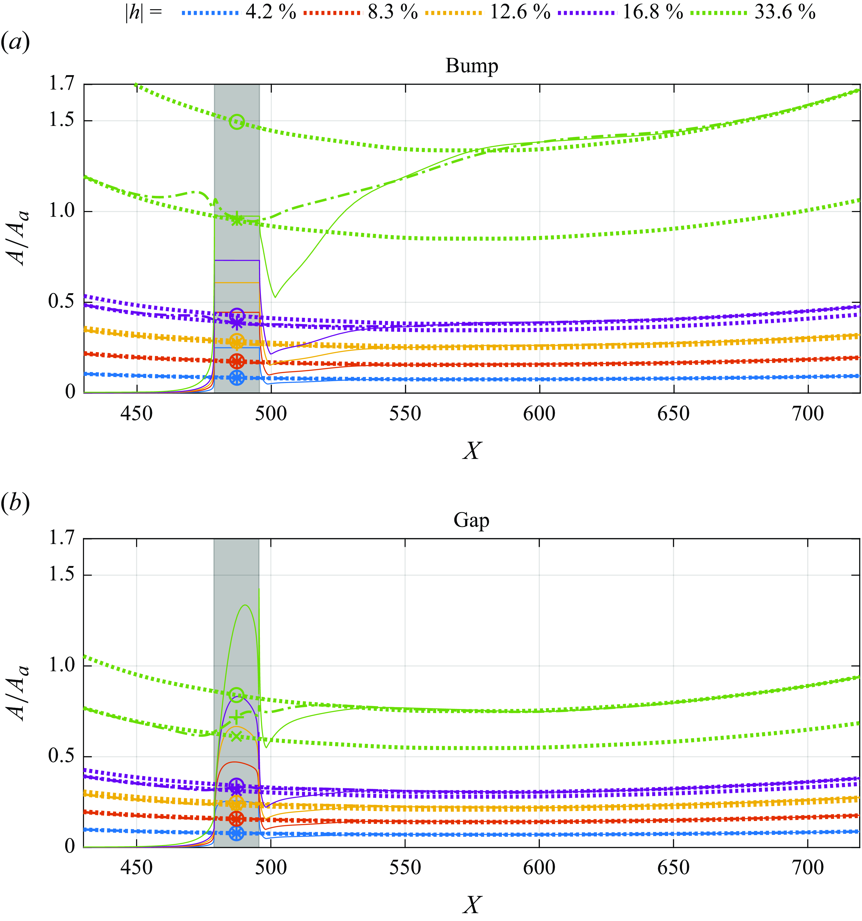
Receptivity maximum amplitudes
 $A_{rc}$
(
 ) for different bump heights and gap depths normalised only by
 $A_{a}$
. The figures also display
 $A_{rg}$
(
 ) and
 $A_{sm}$
(
 ), which were positioned vertically according to our procedure. The symbols are the receptivity estimate according to procedure 1 (
 $\circ$
), procedure 2 (
 $+$
) and procedure 3 (
 $\times$
). The grey rectangle in the background represents the roughness position.
 ${\textit {Re}}_{\delta ^*_b} = 1414$
,
 $M\!a = 0.1$
,
 $A_a = 3.16\times 10^{-5}$
and
 $F = 25.85 \times 10^{-6}$
.

Evolution of the maximum amplitudes of
 $A_{rc}$
() for different bump heights (a) and gap depths (b) normalised by
 $A_{a}$
and
 $|h|$
. The figures also display
 $A_{rg}$
() and
 $A_{sm}$
(). The symbols are the receptivity estimate according to procedure 1 (
 $\circ$
), procedure 2 (
 $+$
) and procedure 3 (
 $\times$
).

Zoomed views of figure 13.

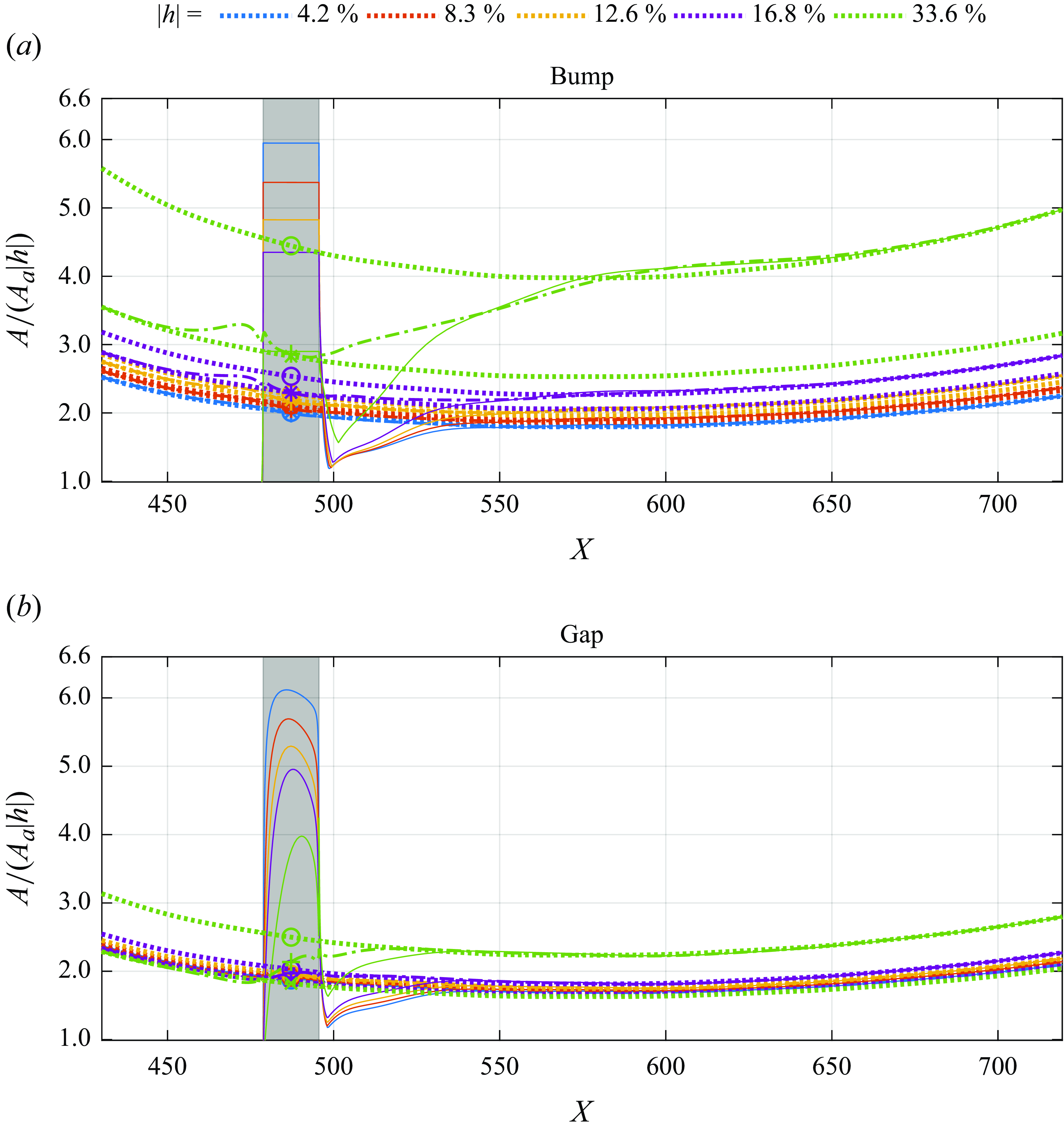
The results shown in figure 11 do not represent estimates of the receptivity amplitude at the roughness element. For this estimate, procedures like 1–3 would be needed. Figure 12 displays, for several bump heights (figure 12
a) and gap depths (figure 12
b) the estimates of receptivity amplitude for the 3 procedures discussed (see figure 3). We present these results for completeness, but for our discussion they are more meaningful if normalised by
 $h$
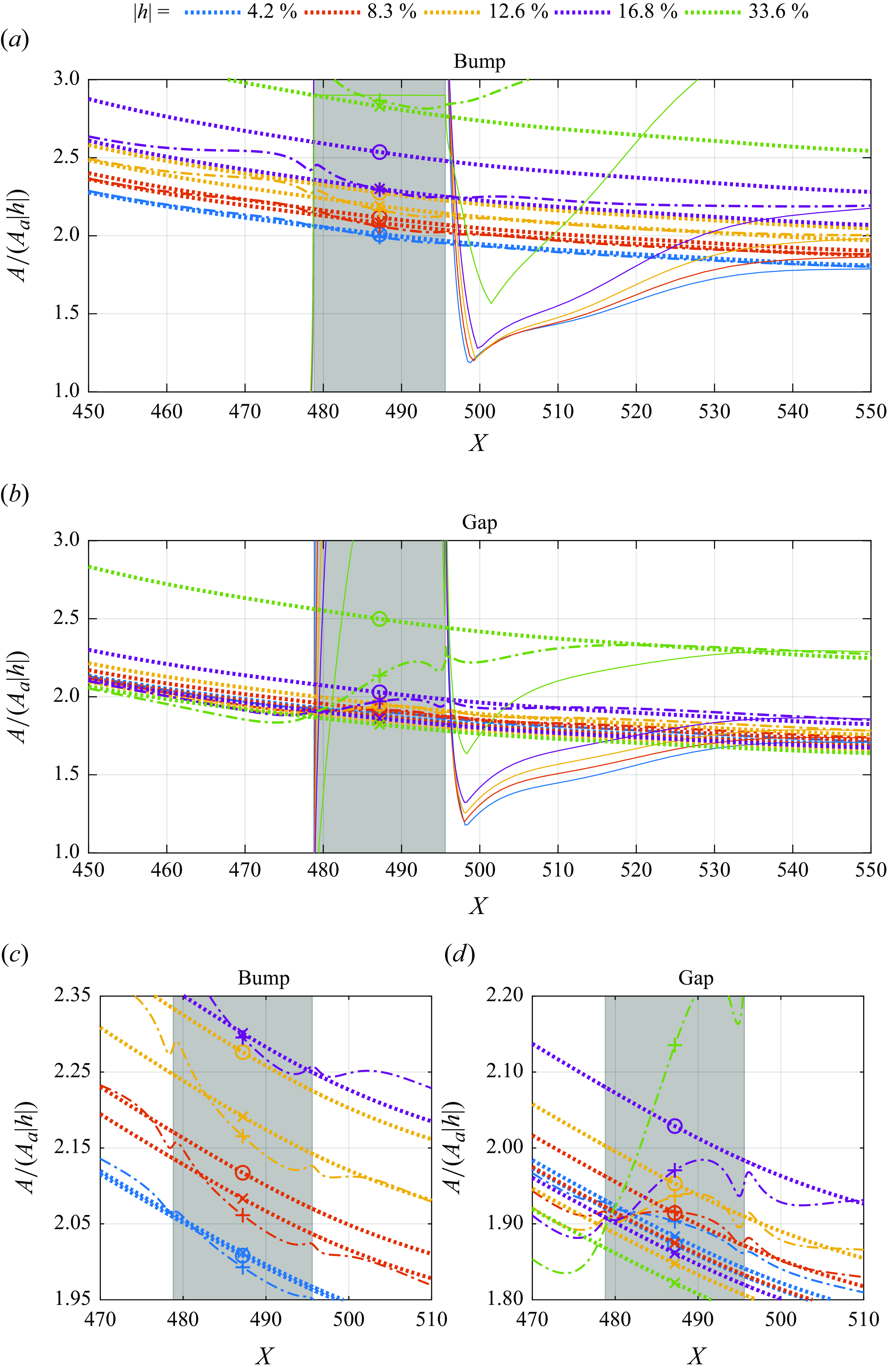
, figure 13. Figure 14 display zoomed versions of figure 13.
In figure 13 it is possible to notice that at
 $|h|=33.6\,\%$
the effect of the bump or the gap on the TS wave evolution is large and leads to very different estimates from procedure 1 relative to the other two (see figure 3). At
 $|h|=33.6\,\%$
, for bump procedures 2 and 3 give similar results, while for the gap it is not the case. For
 $|h|=16.8$
and below, the results from the different procedures would not differ substantially for bumps, see the zoomed-in picture, figure 14(c). However, for gaps, figure 14(d), procedure 2 would lead to substantial differences relative to procedure 3.
The collapse of the solid lines in figure 13 indicates a linear scale with bump height or gap depth. The figure shows that there is a minimum of the solid curves just downstream of the roughness. For the bumps, up to
 $h=16.8\,\%$
, the results almost collapse at the minimum. After that, the curves diverge. For the gap, the collapse at the curve minima is not as good as for the bumps, but in the evolution, the curves do not show strong divergence. Also interesting is that for
 $h$
up to
 $\pm 16.8$
the minima of the curves are similar for bumps and gaps, roughly between 1.2 and 1.3. For
 $|h|=33.6\,\%$
the results differ more substantially. The minimum of the curves is much higher. For the bump, the location of the minimum is shifted downstream.
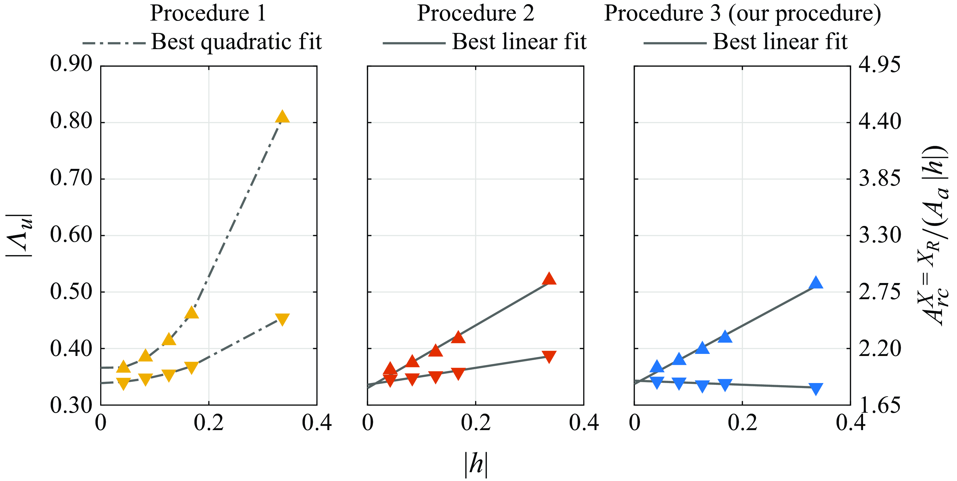
Figure 15 presents the receptivity amplitude and efficiency function for bumps and gaps obtained by the different procedures. The results are normalised by
 $h$
. The figure also gives the efficiency function. The receptivity for gaps is substantially smaller than for bumps even for very small roughness elements. Best linear or parabolic fits are provided as well. In this plot, the linear fits indicate that the relationship between the receptivity efficiency function and the
 $|h|$
follows a second-order polynomial. This situation is seen for procedures 2 and 3. For these procedures, the results converge if extrapolated to
 $h=0$
. This convergence is consistent with a linear regime for infinitesimal roughness elements which is expected to exist, but which, strictly speaking, only applies in that limit.
Overall, these results indicate both the quality of the numerical results and the consistency of procedures 2 and 3 for the estimation of the receptivity amplitude. Procedure 1 does not remove the effect of the roughness on the evolution of the TS wave, in other words, it does not isolate the receptivity process. While for bumps procedure 2 and 3 give similar results, for the gaps even the trend is different. Note that in this plot a linear scaling with
 $h$
would be represented by a horizontal line. For procedure 2 the receptivity grows superlinearly with
 $h$
while for procedure 3 there is a saturation, a sublinear scaling with
 $h$
.
Efficiency function absolute value (
 $|\Lambda _u|$
) and normalised receptivity amplitude at the bump (
 ) and gap (
 ) centre estimated by different procedures:
 ${\textit {Re}}_{\delta ^*_b} = 1414$
,
 $M\!a = 0.1$
,
 $A_a = 3.16\times 10^{-5}$
and
 $F = 25.85 \times 10^{-6}$
.

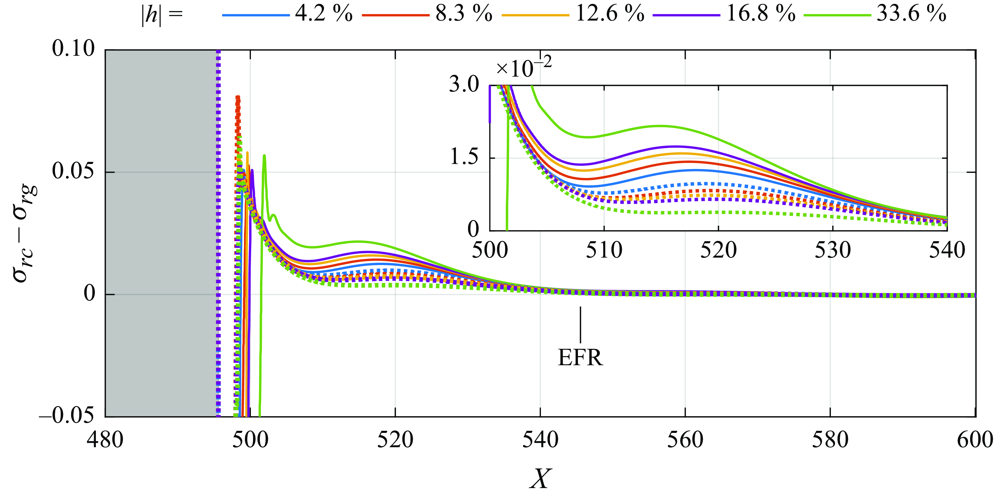
Figure 16 shows what we named deviatory growth rates, the growth rate of the disturbances calculated from the results of figure 12 subtracted from the growth rate of the corresponding
 $TS_{rg}$
. It should be emphasised that the expression growth rate is here used in a rather loose sense because in the formation region (roughly up to
 $X=545$
) the disturbances are non-modal. This difference represents the growth rate of the build-up of the TS wave that characterises the formation region. The evolution is similar for all heights and depths. Just downstream of the bump, the growth rates reach a maximum and then decay. They experience a second local maximum and decay to zero. For all
 $h$
the curves fall to zero at the same position, approximately
 $50 \delta ^*_{b}$
from the trailing edge of the bump (roughly 90 % of a TS wavelength of that frequency). It indicates that the length of the formation region is the same for all
 $h$
covered. For the bumps the global maximum shifts downstream as
 $h$
increases. Comparing with results from figure 10 we see that the maximum is close to the reattachment of the boundary layer, which moves downstream with
 $h$
. The flows in gaps show no discernible separation at the trailing edge and the global maximum occurs at the same location for all depths. Despite the shift in the global maximum, even for
 $h=33.6\,\%$
the formation region ends at the same location as the other bumps and the gaps.
Deviatory growth rates for bumps () and gaps ().

In figure 16, if the curves for the bumps were shifted to align their maxima, the collapse in that region would be similar to that for the gaps. The difference in the behaviour of gaps and bumps lies mostly in the second maxima. The figure shows that for the bumps the maxima increases with
 $h$
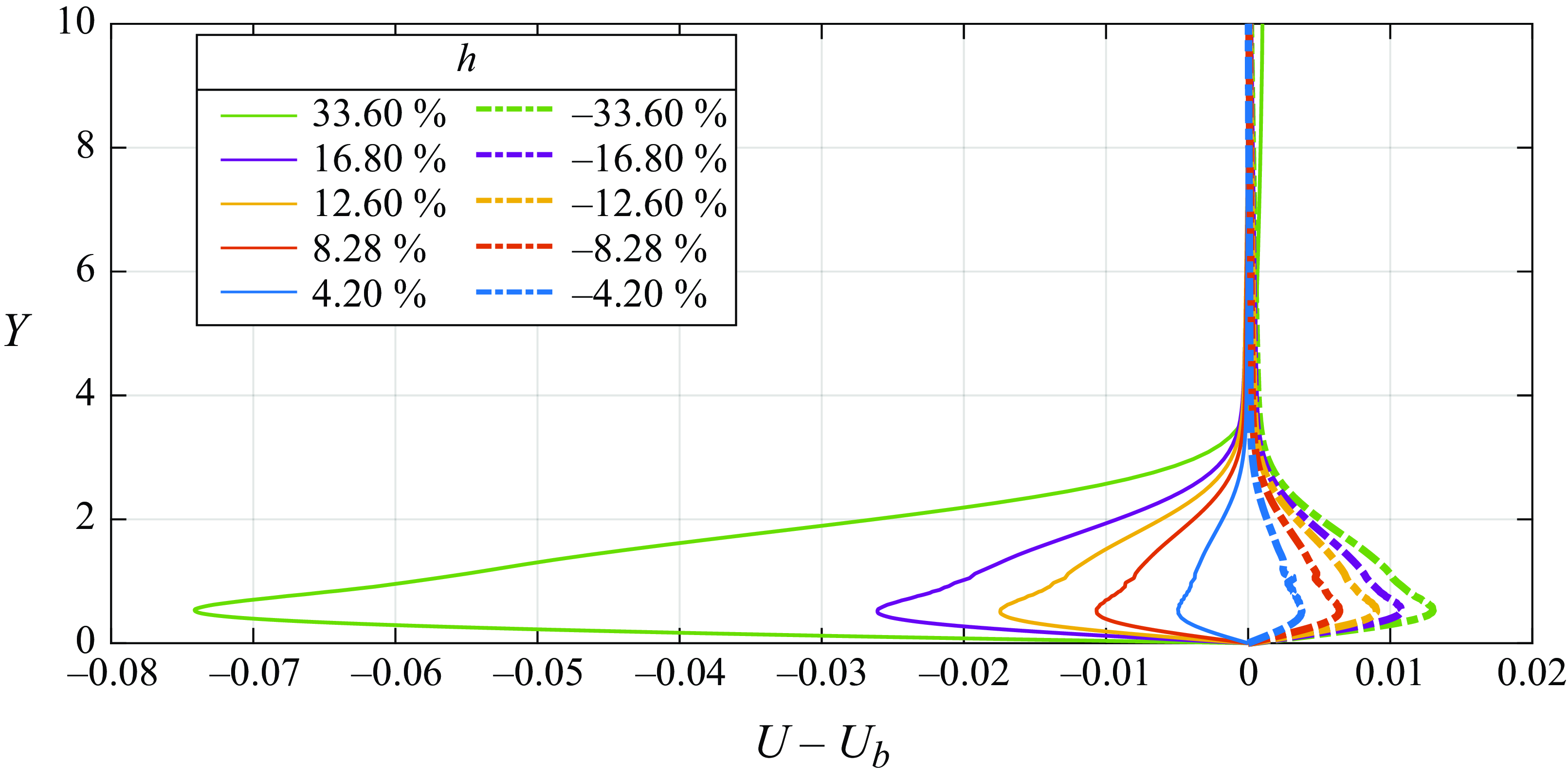
, while for the gaps the opposite occurs. In some sense, this situation embodies the concept that the gap has to be opposite to a bump. Figure 17 shows what we refer to as deviation profiles, the difference between the profiles in the roughness element wake and the Blasius profile, which, for the current analysis, was obtained from the smooth plate simulations. The deviation profiles show more clearly the differences between gaps and bumps. We see that for the bump there is a velocity deficit that increases with bump height, while for the gap, there is a velocity excess. For the bumps, the velocity profiles resemble adverse pressure gradient profiles which enhance the growth of the TS waves, while for the gap it is the opposite. It is conjectured that a similar effect enhances the outcome of the formation region. It may be part of the explanation for the different behaviour observed. This opposite behaviour is captured by procedure 3 which shows a sublinear scaling for the gaps with respect to depth. We claim that procedure 3 captures these details because it is not vulnerable to the larger oscillations observed for the gaps (figure 14
d), or vulnerable to the profile distortions shown in figure 4.
Deviation profiles for bumps () and gaps () at X = 510.

4.3. Compressibility effects
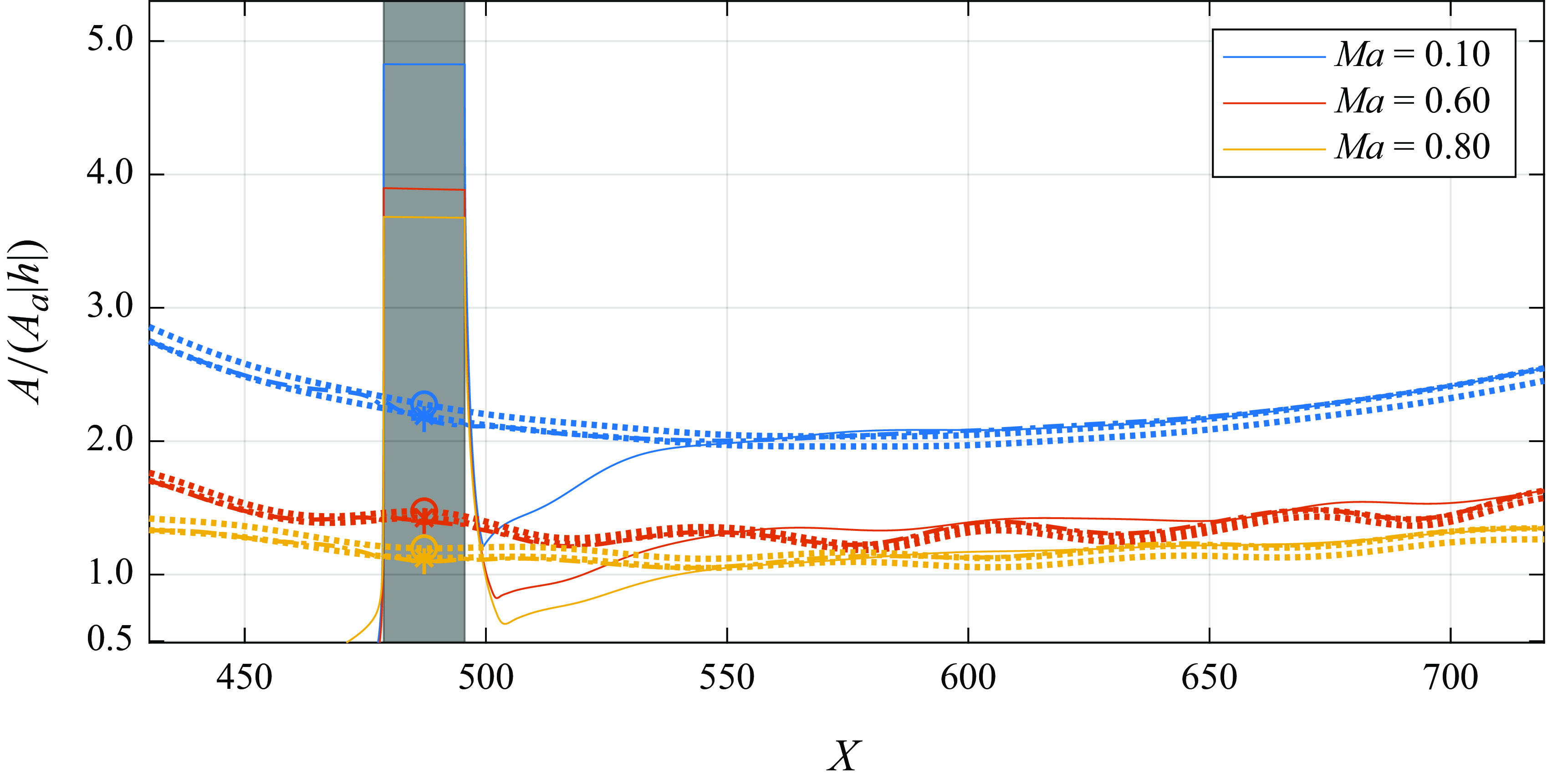
Figure 18 depicts the evolution of the
 $TS_{rc}$
and their respective
 $TS_{rg}$
and
 $TS_{sm}$
for different
 $M\!a$
. For higher
 $M\!a$
the evolution displays oscillations. These oscillations are associated with the acoustic waves produced by the suction and blowing on the wall that generate the TS waves needed for the analysis. This waviness appears on the
 $TS_{rg}$
and
 $TS_{sm}$
and as a consequence on the
 $TS_{rc}$
as well. We verified (Dos Santos Reference dos Santos2022) that this waviness can be substantially reduced if, for example, we excite the waves with a streamwise velocity fluctuation instead of the suction and blowing. The streamwise velocity excitation constitutes an acoustic dipole which is much less acoustically efficient in the subsonic regime. We can also reduce these fluctuations if we base the receptivity amplitude estimates on the wall-normal velocity component of the TS wave (dos Santos Reference dos Santos2022), because the acoustic wave has only a small projection in the wall-normal direction. We refrained from using these alternative approaches because these oscillations do not affect the results beyond the accuracy of the computations. Moreover, using alternative approaches would require details that would unnecessarily lengthen the paper.
Effect of
 $M\!a$
on the receptivity of bump with
 $h = 12.6\,\%$
,
 $12.15\,\%$
and
 $11.89\,\%$
for
 $M\!a = 0.1$
,
 $0.6$
and
 $0.8$
, respectively. The curves showed in the figure are
 $A_{rc}$
(),
 $A_{rg}$
() and
 $A_{sm}$
(). Here
 $A_{sm}$
was adjusted with our procedure. The symbols are the receptivity estimate according to procedure 1 (
 $\circ$
), procedure 2 (
 $+$
) and procedure 3 (
 $\times$
). The grey rectangle in the background is the position of the roughness. Here
 ${\textit {Re}}_{\delta ^*_b} = 1414$
,
 $A_a = 3.16\times 10^{-5}$
and
 $F = 25.85 \times 10^{-6}$
.

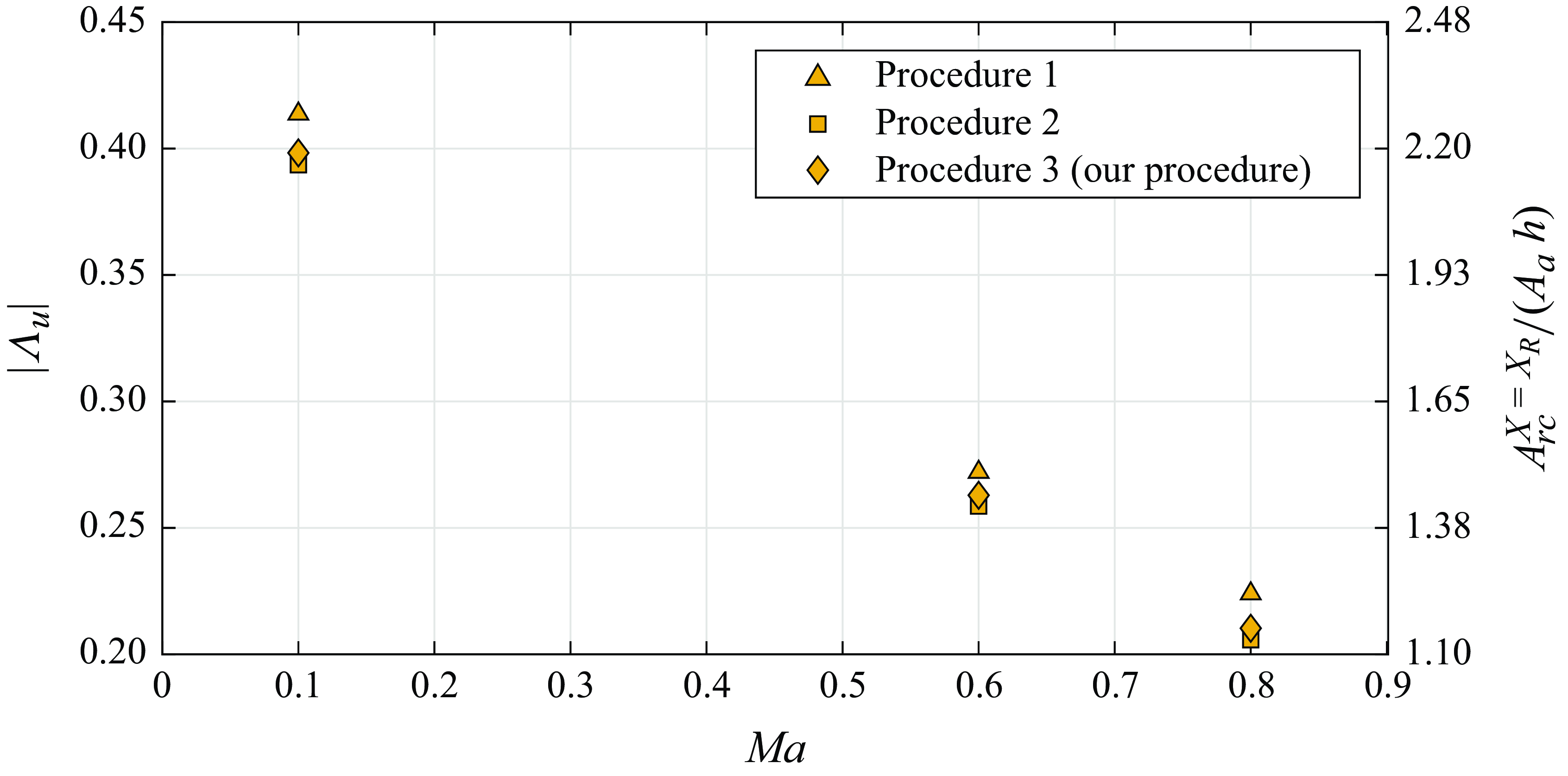
Efficiency function absolute value (
 $|\Lambda _u|$
) and receptivity amplitude at the centre of bumps with
 $h = 12.60\,\%$
,
 $12.15\,\%$
and
 $11.89\,\%$
for
 $M\!a - 0.1$
,
 $0.6$
and
 $0.8$
, respectively. Here
 ${\textit {Re}}_{\delta ^*_b} = 1414$
,
 $M\!a = 0.1$
,
 $A_a = 3.16\times 10^{-5}$
and
 $F = 25.85 \times 10^{-6}$
.

Using our procedure we calculated the receptivity amplitude shown in figure 19. Results show that receptivity decreases substantially with
 $M\!a$
(a factor of approximately 2 from
 $M\!a=0.1$
to
 $0.8$
). The receptivity results from Raposo et al. (Reference Raposo, Mughal and Ashworth2019) for acoustic waves over surface roughness (figure 5a from their paper) decrease by a factor of approximately
 $2.5$
for flow parameters similar to ours (in their paper,
 ${\textit {Re}}_{\delta ^*_b} = 1400$
and
 $\mathcal {F} = 20 \times 10^{-6}$
and
 $M\!a$
also from
 $0.1$
to
 $0.8$
). The decrease in the receptivity amplitude observed here is hence generally in line with the results from Raposo et al. (Reference Raposo, Mughal and Ashworth2019). We call attention to the fact that as
 $M\!a$
increases the boundary layer becomes thicker. We did not take this effect into account when performing the simulations, and for
 $Ma=0.8$
this effect reduced the bump height to
 $11.89\,\%$
. It is a small value that does not affect the general conclusions.
4.4. Effect of acoustic wave amplitude
The effect of the amplitude of the acoustic wave on receptivity is still under debate. Saric (Reference Saric1994) suggested the receptivity scales nonlinearly with the acoustic wave amplitude in the range between
 $90\,{\rm d}B$
and
 $100\,{\rm d}B$
. Placidi et al. (Reference Placidi, Gaster and Atkin2020) also observed a nonlinear behaviour in the range between
 $70\,{\rm d}B$
and
 $80\,{\rm d}B$
. However, Nayfeh & Ashour (Reference Nayfeh and Ashour1994) note that in Saric (Reference Saric1994) the TS wave amplitude did not approach zero for bumps with vanishing heights. Nayfeh & Ashour (Reference Nayfeh and Ashour1994) argue that TS waves were present upstream of the bump in Saric (Reference Saric1994), presumably owing to the receptivity at the experimental model leading edge. By adjusting the amplitude of a prior existing TS wave, Nayfeh & Ashour (Reference Nayfeh and Ashour1994) accurately reproduce the results of Saric (Reference Saric1994) with a model in which the receptivity scaled linearly with the amplitude of the acoustic wave. It is evident that the argument of Nayfeh & Ashour (Reference Nayfeh and Ashour1994) may also be applicable to the results of Placidi et al. (Reference Placidi, Gaster and Atkin2020).
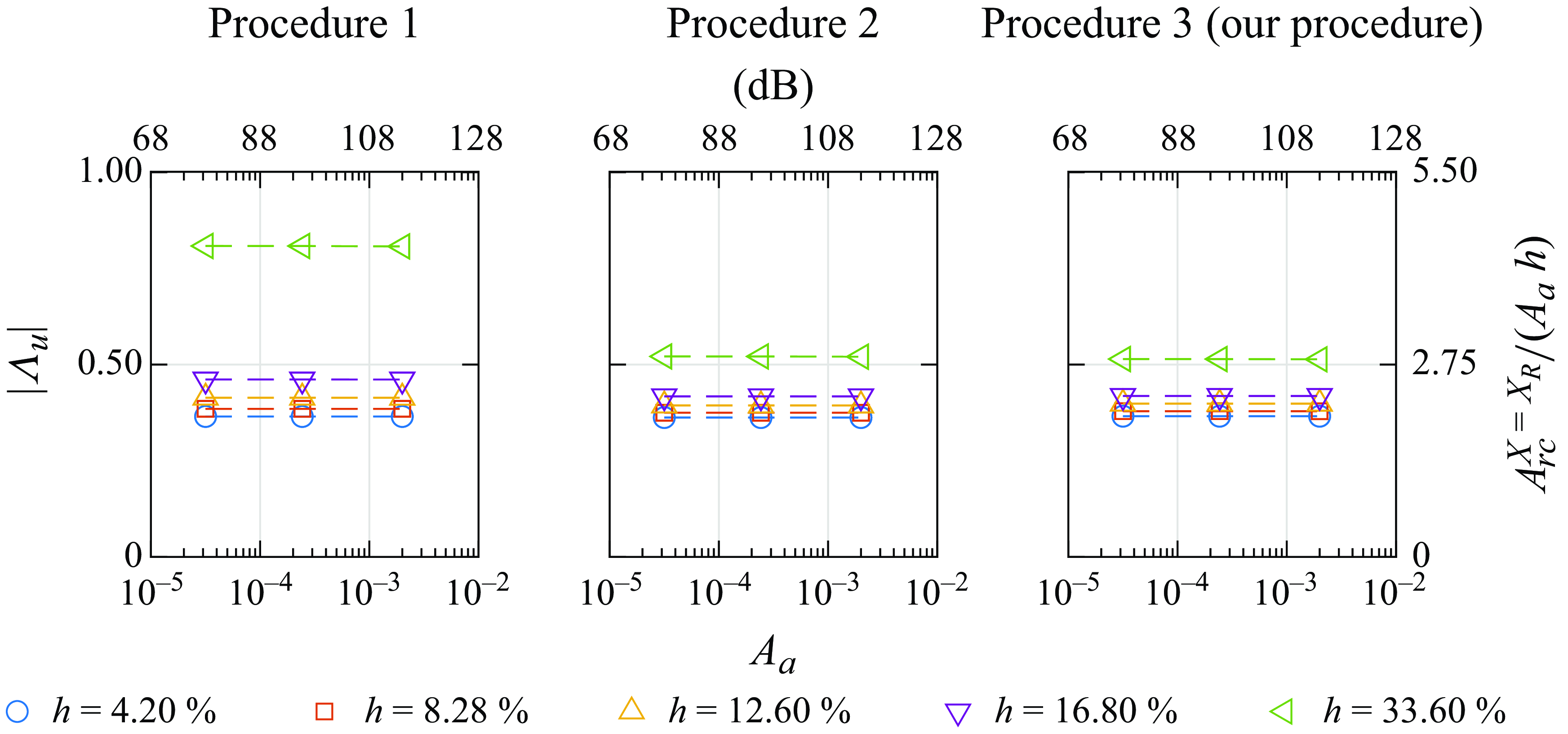
Efficiency function absolute value (
 $|\Lambda _u|$
) and receptivity amplitude at roughness centre as a function of acoustic wave amplitude
 $A_a$
for different bump heights from different procedures. The acoustic wave amplitude is also presented as sound pressure level (dB) with the flow parameters from Placidi et al. (Reference Placidi, Gaster and Atkin2020) (i.e.
 $U_{\infty }^* = 18.42 \, \rm m\,s^-{^1}$
and acoustic impedance of air at
 $30^{\circ } = 406.5 \, {\rm Pa} \, \rm s\,m^-{^1}$
), and reference pressure
 ${P}^{*}_0 = 20 \, \mu {\mathrm {Pa}}$
.
 ${\textit {Re}}_{\delta ^*_b} = 1414$
,
 $M\!a = 0.1$
and
 $F = 25.85 \times 10^{-6}$
. Some axes labels have been omitted to improve readability.

Our results for the receptivity amplitude for different acoustic wave amplitudes are plotted in figure 20 for bumps with different heights. In the acoustic amplitude range investigated, which includes the range from Nayfeh & Ashour (Reference Nayfeh and Ashour1994), Saric (Reference Saric1994) and Placidi et al. (Reference Placidi, Gaster and Atkin2020), the receptivity scales linearly with the acoustic wave amplitude. In our simulations, the handling of the plate leading edge prevented TS waves upstream of the bump and, hence, corroborated the arguments raised by Nayfeh & Ashour (Reference Nayfeh and Ashour1994).
5. Conclusion
The paper reported on a high-fidelity simulation investigation of acoustic receptivity of TS waves due to bumps and gaps. The bumps and gaps were rectangular with sharp edges, and the computational grids were body-fitted to the roughness element. The results were successfully compared with linear theories and numerical simulations that represent the roughness with a Taylor expansion (with grids not fitted to the roughness shape). Comparison with experiments was also successful if the results were adjusted to compensate for a small pressure gradient typical for that experimental set-up on the flap plate. The roughness elements were very small, hence we placed great emphasis on the accuracy of the results. The grid independence tests indicated an accuracy of approximately
 $4\,\%$
of the amplitude of the TS wave.
The evolution of the TS wave produced by the receptivity at the roughness is affected by the distortions that the roughness element causes on the velocity field downstream. In the current study, two procedures from the literature were used to estimate the receptivity, procedure 1, that does not account for the effect mentioned above, and procedure 2, that does. The latter requires a second simulation, one that simulates the interaction of a TS wave with a roughness. However, owing to non-parallel effects at the roughness location, the disturbance there is non-modal. It does not readily provide a TS wave from which a TS wave amplitude can be obtained. We then proposed another procedure (procedure 3) to overcome these difficulties. The procedure includes a third simulation, one that simulates the evolution of a TS wave on a smooth surface. The procedure was particularly relevant for estimating the receptivity of gaps. The results show that the bump is significantly more receptivity than the gaps. At
 $h=\pm 4\,\%$
the bump had a receptivity amplitude almost
 $10\,\%$
higher than the gap, as measured by procedure 3. For procedure 2, the receptivity of bumps and gaps scales superlinearly with
 $|h|$
. For procedure 3 the receptivity for bumps scales superlinearly with
 $|h|$
while for gaps it scales sublinearly. For procedures 2 and 3, the receptivity estimates for gaps and bump converge to each other for vanishingly small roughness elements, a result that is expected on the grounds that for small roughness elements the receptivity should scale linearly with
 $h$
.
Our results indicate a region downstream of the roughness where the TS wave builds-up, and which we call the ormation region. Plots of growth rates extracted from the TS wave evolution computed numerically indicate the length of the formation region does not depend on
 $h$
and is the same for bumps and gaps. These plots indicated that within the formation region, the growth rate depends on
 $h$
. It increases with bump height, but reduces with gap depth. It was also found that within the formation region, the boundary layer profiles are distorted by the roughness element. For bumps, there is a deficit in the profile that increases with bump height. Hence, the bump wake profiles resemble adverse pressure gradient ones, which enhance the TS wave instability. For the gap a profile excess is formed, resembling a favourable pressure gradient profile. Consistently, the profiles that enhance the TS instability also enhance the receptivity output. One expects that in some way a gap should display a behaviour opposite to that of the bump. Procedure 3 captures this trend, by indicating either superlinear or sublinear scalings.
Up to the heights or depths of
 $12.6\,\%$
, the base flow displayed only a very short, essentially negligible, separation bubble. For bump height
 $h =33.6\,\%$
, the base flow displayed a much longer separation bubble. This separation altered the details of the receptivity process, nevertheless, it did not alter the scaling of the receptivity with respect
 $h$
.
We also investigated the effect of compressibility on the receptivity process. The results showed that the receptivity reduced substantially with Mach number, in line with previous studies. The effect of acoustic wave amplitude was also tested. It is still a controversial issue. Experiments have indicated that, in the range
 $70\,{\rm d}B$
to
 $100\,{\rm d}B$
the receptivity scaled nonlinearly with acoustic wave amplitude. However, Nayfeh & Ashour (Reference Nayfeh and Ashour1994) argued that receptivity at the experimental model leading edge could have contaminated the results. Our receptivity amplitudes scaled linearly with acoustic wave amplitude in the same acoustic wave amplitude range. Since our results are not subject to leading edge contamination, they lend support to the arguments of Nayfeh & Ashour (Reference Nayfeh and Ashour1994).
Acknowledgements
We thank the University of Liverpool for the access to the Barkla cluster, provided by Professor V. Theofilis. We also thank the Centre for Mathematical Sciences Applied to Industry (CeMEAI), funded by São Paulo Research Foundation (FAPESP/Brazil), grant 2013/ 07375–0 and led by Professor J.A. Cuminato, for access to the Euler cluster. dos Santos, P.H.R. was sponsored by CAPES/Brazil grant no. 88882.379188/ 2019–01 and by FAPESP/Brazil grant no. 2020/ 04413–1. Himeno, F.H.T. was sponsored by FAPESP/Brazil grant no. 2018/ 02542–9. Mathias, M.S. was sponsored by FAPESP/Brazil grant no. 2018/ 04584–0. Medeiros, M.A.F. was sponsored by National Council for Scientific and Technological Development (CNPq/Brazil), grant no. 307956/ 2019–9. The work also benefited from the US Air Force Office of Scientific Research (AFOSR) grant FA 9550–18- 1–0112, managed by Dr G. Andersen and Lt. Col. D. Montes and grant FA 9550–23- 1–0030, managed by Dr R. Greenwood.
Declaration of interests
The authors report no conflict of interest.
Appendix A
A.1. Grid requirements and accuracy
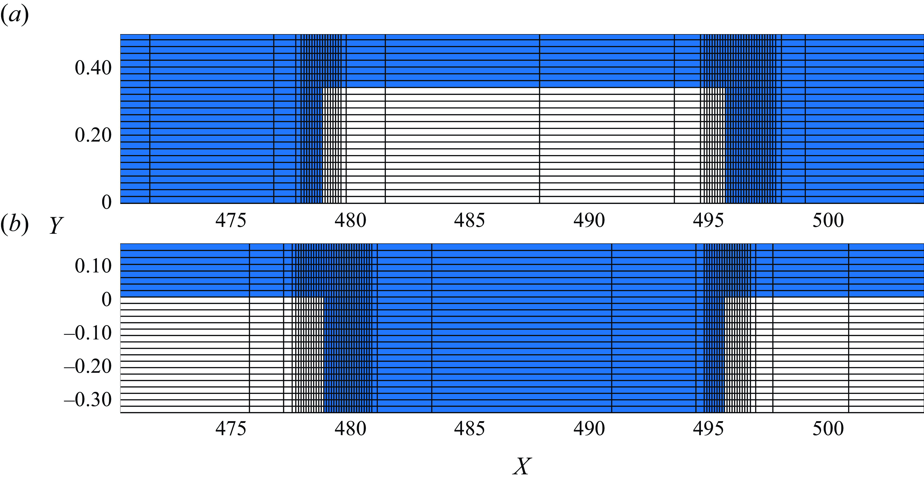
The structured mesh used occupied a rectangular domain with grid stretching implemented in both streamwise (
 $X$
) and wall-normal (
 $Y$
) directions, as illustrated in figure 21.
Structured meshes employed in the present DNS for (a) bump and (b) gap for
 $h = \pm 33.6\,\%$
. The figures illustrate the mesh density through a line drawn every second grid point in the Y direction and every eleventh grid point in the X direction.

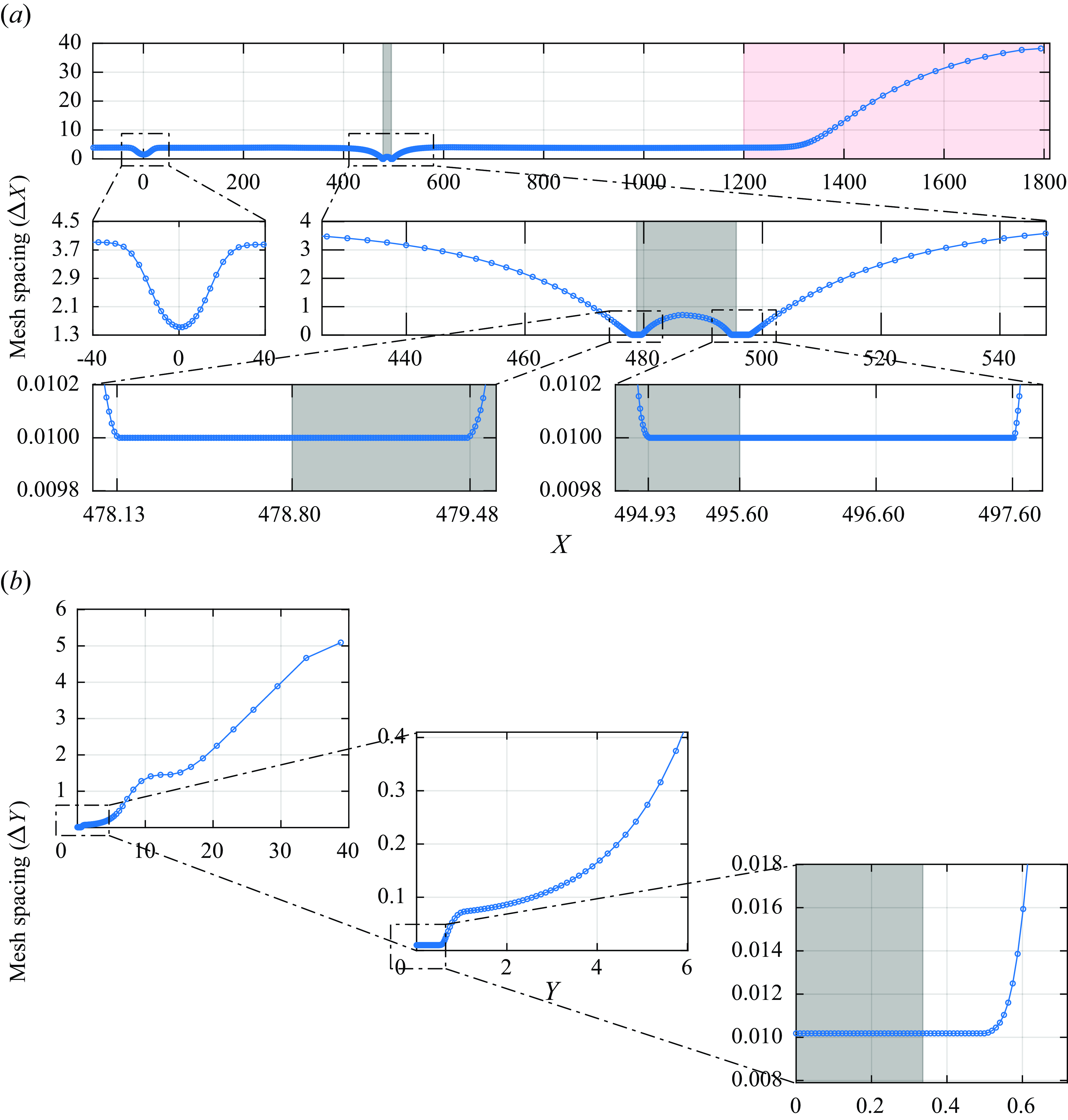
The code uses structured mesh in a rectangular domain with grid stretching in both X and Y directions. Figure 22 displays the mesh. The grid is much finer near the wall and at the roughness location. The stretching is over two-orders of magnitude. At the roughness the grid is essentially the same in the X and Y directions. At least five grid points were needed along the bump height or gap depth.
Mesh used in the simulation in the (a) streamwise and (b) wall-normal directions, respectively. There is stretching in both directions. The grey rectangle in the background is the position of the roughness and the red one is part of the buffer zone.

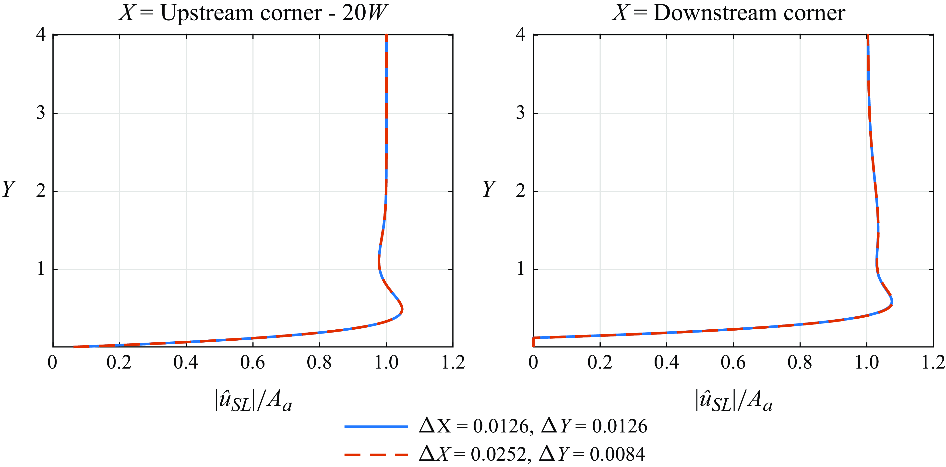
Figure 23 shows the Stokes layer profile for different mesh refinements and positions on the plate. No discernible difference in the Stokes layer profile is present, indicating grid independence.
Stokes layer profile (
 $|\hat {u}_{SL}|$
) obtained at different streamwise positions for different mesh refinements:
 $h = 12.6\,\%$
;
 ${\textit {Re}}_{\delta ^*_b} = 1414$
;
 $M\!a = 0.1$
;
 $A_a = 3.16\times 10^{-5}$
;
 $F = 25.85 \times 10^{-6}$
.

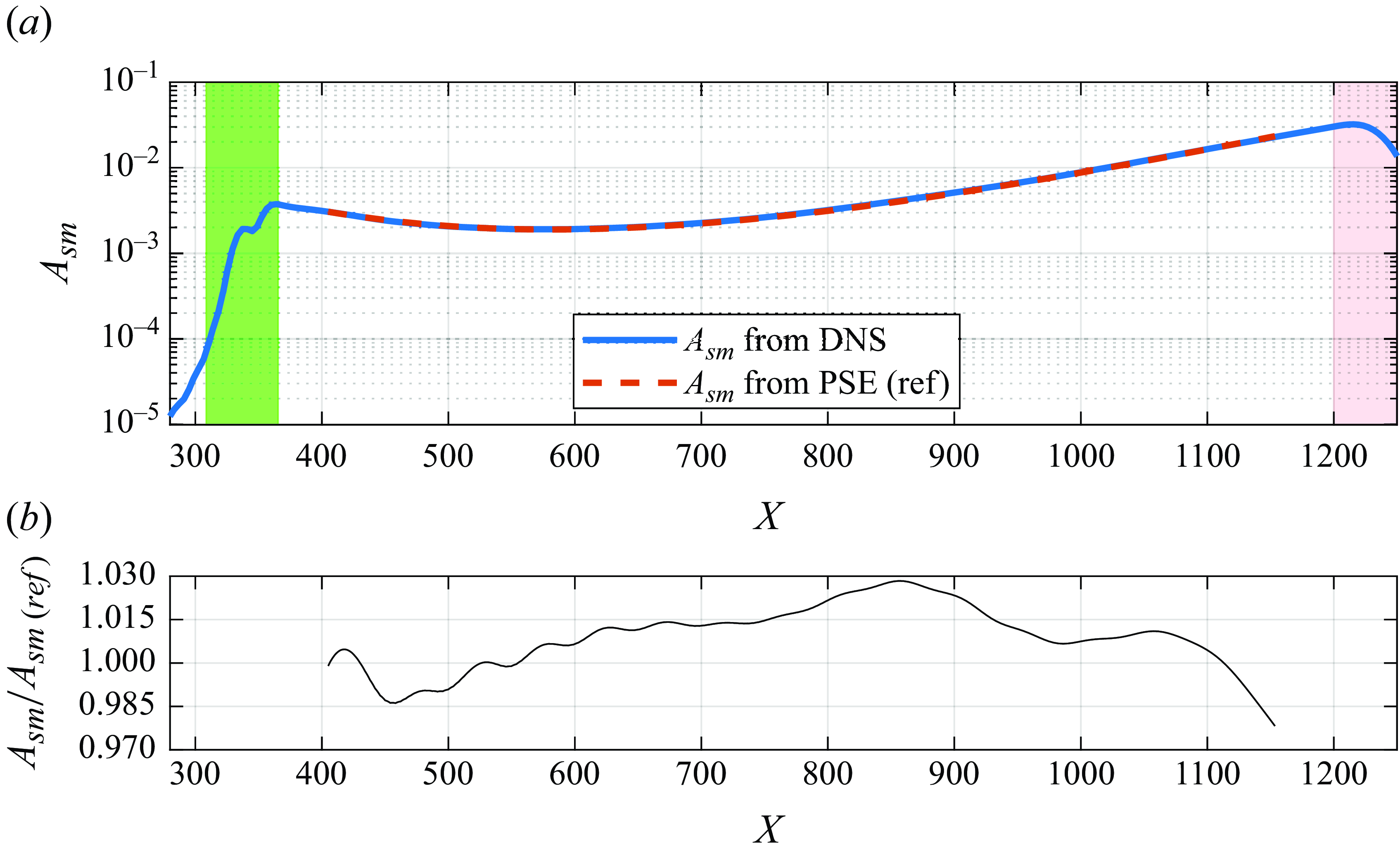
The figure 24(a) shows the amplitude evolution of a TS wave of small amplitude computed by our simulations in comparison with linear PSE results. Figure 24(b) indicates that the error remains below 3 %, which is within the other bounds established. The agreement is therefore good and validates our simulations. It also shows that in two dimensions the waves remained in the linear regime up to fairly large amplitudes.
(a) The
 $TS_{sm}$
amplitude evolution for
 $M\!a = 0.1$
from the present DNS and obtained by PSE computations. (b) The ratio between
 $TS_{sm}$
amplitudes. The green rectangle in the background is the position of the source of the TS wave and the red one is part of the buffer zone. Here,
 ${\textit {Re}}_{\delta ^*_b} = 1414$
,
 $M\!a = 0.1$
and
 $F = 25.85 \times 10^{-6}$
.

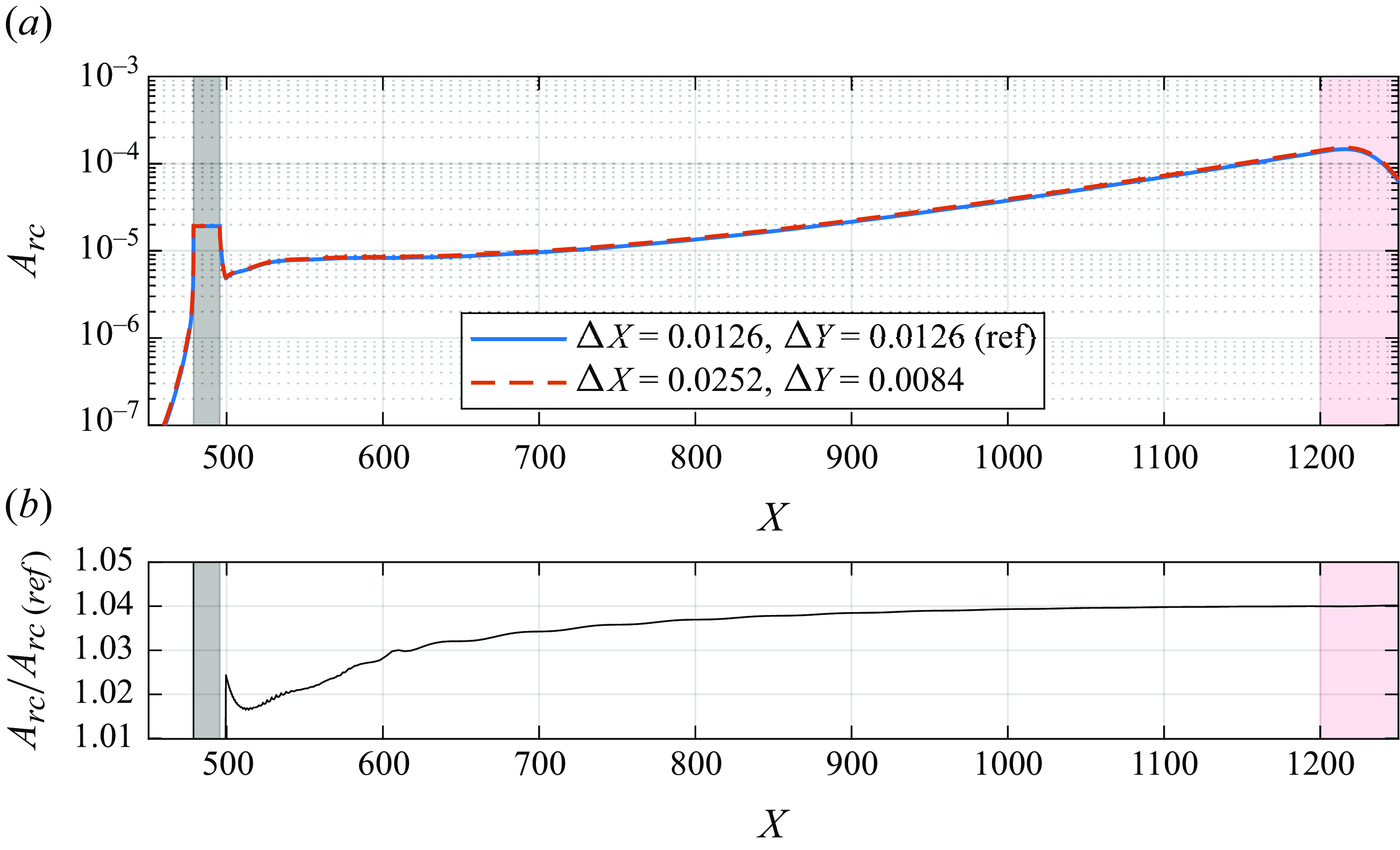
For the receptivity process, the mesh independence is demonstrated in figure 25, where the mesh is refined in either X or Y direction. Figure 25(a) shows TS wave evolutions and figure 25(b) depicts the ratio between the TS wave amplitude for different mesh sizes along the wave evolution. The difference is below 4 %. We took this value as representative of the numerical uncertainty of the
 $TS_{rc}$
wave with regard to mesh, and considered it enough for our current interest. For the
 $TS_{rg}$
the same grid was used with the same level of accuracy. For the
 $TS_{sm}$
the same accuracy could be achieved with a much less refined grid.
The
 $TS_{rc}$
amplitude evolution for different mesh refinement levels. Panels (a) and (b) refer to TS wave evolutions and ratio between evolutions, respectively. The grey rectangle in the background is the position of the roughness and the red one is part of the buffer zone.

A.2. Effectively incompressible Mach number
The DNS code used was implemented with compressible governing equations, enabling the study of the receptivity sensitivity to
 $M\!a$
. Simulations at the experimental
 $M\!a$
would be very expensive, since the time step required to maintain numerical stability would be very small. Therefore, it is interesting to find the highest
 $M\!a$
for which the flow can still be regarded as incompressible.
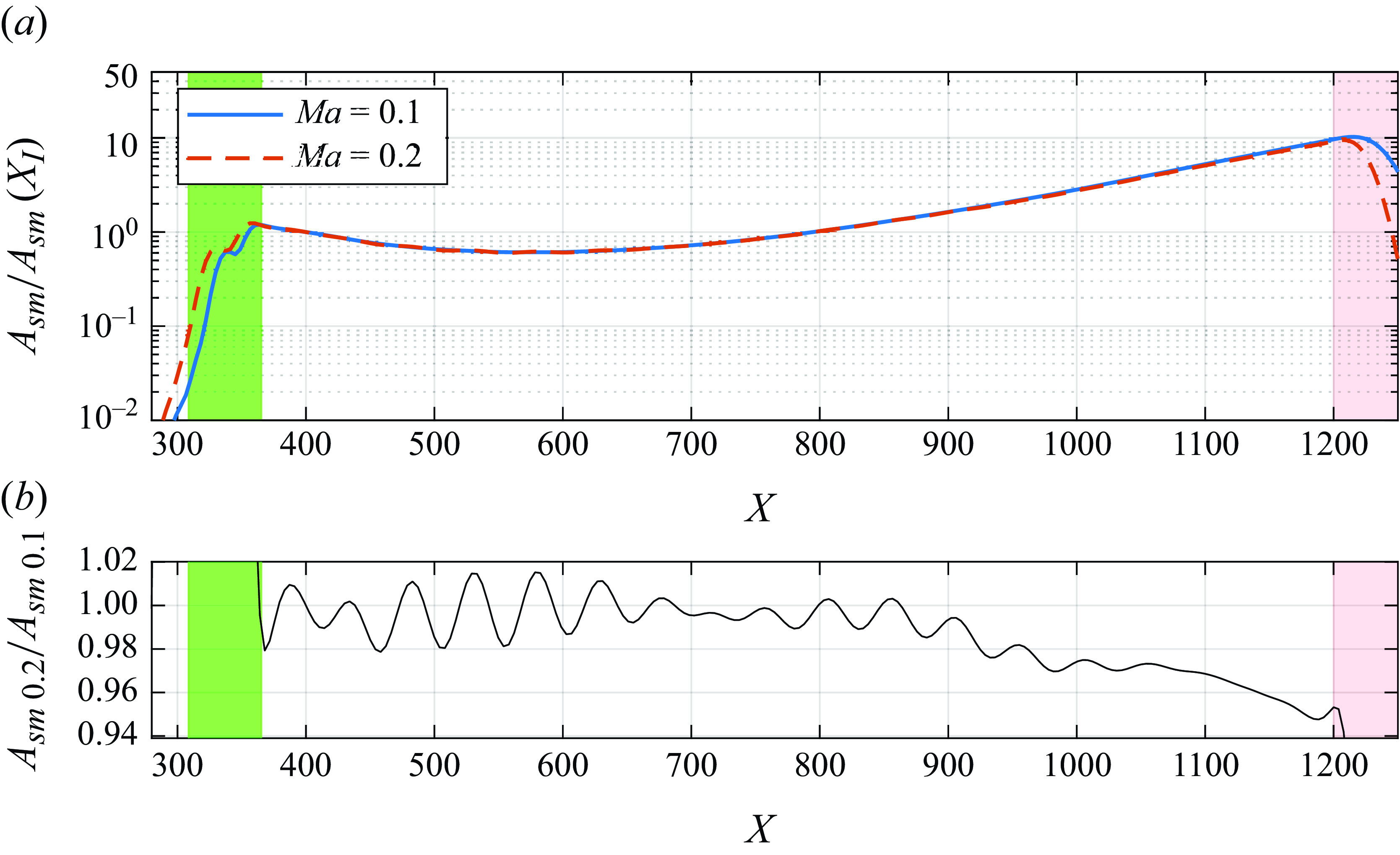
Figure 26 displays a comparison between the evolutions of the
 $TS_{sm}$
with
 $Ma = 0.1$
and
 $0.2$
. Figure 26(b)shows that the difference is approximately 4 % over the wave evolution, which is similar to the numerical precision, as discussed above. In the study
 $M\!a=0.1$
was used.
(a) The
 $TS_{sm}$
amplitude evolution for
 $M\!a = 0.1$
and
 $0.2$
normalised by the respective amplitudes at the first branch (
 $X_I$
). (b) The ratio between
 $TS_{sm}$
amplitudes at
 $M\!a = 0.2$
and
 $M\!a = 0.1$
. The green rectangle in the background is the position of the source of the TS wave and the red one is part of the buffer zone.