


1. Introduction
In global tectonics, the lithosphere-asthenosphere boundary (LAB) is one of the most important interfaces. It is a first-order structural discontinuity that accommodates differential motion between tectonic plates and the underlying mantle (Eaton et al. Reference Eaton, Darbyshire, Evans, Grütter, Jones and Yuan2009). The boundary separates the cooler and mechanically more rigid lithosphere from the ductile asthenosphere. The terms lithosphere and asthenosphere themselves were defined by Barrel (Reference Barrell1914), who already at that time assumed that there must be a zone of weakening (asthenosphere) under the solid lithosphere, in which the rock mass can move laterally and thus compensate for changes in the distribution of masses at the surface.
The LAB is determined by the differences between the lithosphere and asthenosphere, which may be caused by variations in grain size, chemical composition, thermal properties and extent of partial melting (e.g., Artemieva and Mooney, Reference Artemieva and Mooney2001). Classically, the LAB is defined thermally, with a gradual transition from the colder conductive lithosphere to the warmer convective asthenosphere beneath (Eaton et al. Reference Eaton, Darbyshire, Evans, Grütter, Jones and Yuan2009). The original seismic definition of the lithosphere was given by Gutenberg (Reference Gutenberg1954) as the high-velocity outer layer of the Earth, underlain by a low-velocity zone or a region where the positive velocity gradient diminishes. The electrical LAB is traditionally identified by a rapid reduction in electrical resistivity at upper mantle depths (Heinson, Reference Heinson1999; Jones, Reference Jones1999). The lithosphere, sensu stricto, is a mechanical boundary layer. The LAB coincides with the top of a zone of decoupling between the lithosphere and asthenosphere, marked by an increased strain rate (e.g., Eaton et al. Reference Eaton, Darbyshire, Evans, Grütter, Jones and Yuan2009). The boundary may also correlate with a downward extinction of seismic anisotropy (e.g., Gaherty and Jordan, Reference Gaherty and Jordan1995) or a change in the direction of anisotropy (e.g., Sebai et al. Reference Sebai, Stutzmann, Montagner, Sicilia and Beucler2006).
Petrological definition of the LAB involves differences in the composition of the mantle at depth (Artemieva, Reference Artemieva2011). The lithospheric mantle is ultramafic and devoid of volatiles and some incompatible elements. The depth to the base of the lithosphere can be determined using the amount of forsterite component in olivine. This is because the partial melting of the primitive mantle leaves behind a composition enriched in magnesium.
Another petrological definition designates the LAB as a phase boundary marking the intersection of the geotherm with the solidus of amphibole (pargasite)-bearing peridotite (Niu and Green, Reference Niu and Green2018). Consequently, the oceanic LAB is petrologically defined by the ∼1100°C isotherm for ocean ages less than 70 Ma and the ∼3 GPa isobar for ages above 70 Ma. This unifying concept explains why the LAB depth increases beneath young ocean floors (<70 Ma) and remains constant afterwards at ∼90 km (Niu and Green, 2018). The LAB intrinsically determined by petrological phase equilibria does not require small-scale convection; however, the small-scale convective heat supply in the asthenosphere (peridotite involving incipient melt) beneath older seafloors provides the heat conductively lost through the lithosphere (pargasite-bearing peridotite without interstitial melt), thus maintaining the heat flow constant.
How to define or estimate LAB depth by various methods with their individual sensitivities and resolution remains under debate.
The history of determining the depth of the LAB and the lithospheric structure in the Carpathian-Pannonian region and surrounding areas is long and rich. After Panza’s (Reference Panza, Galson and Mueller1985) study Europe-wide surface wave study, Babuška et al. (Reference Babuška, Plomerová, Šílený, Froidevaux and Fuchs1987, Reference Babuška, Plomerová and Pajdušák1988) and Babuška and Plomerová (Reference Babuška, Plomerová and Hillhouse1989, Reference Babuška and Plomerová1992) applied the interpretation of teleseismic P-wave delay times to publish the first-ever results of the LAB depth in Central Europe. Subsequently, the seismic methods were supplemented and compared by magnetotelluric sounding measurements (Praus et al. Reference Praus, Pěčová, Petr, Babuška and Plomerová1990) and geothermal modelling (Čermák, Reference Čermák, Bucha and Blížkovský1994; Gordienko and Zavgorodnyaya, Reference Gordienko and Zavgorodnyaya1996). Later, Babuška and Plomerová (Reference Babuška and Plomerová1992), Plomerová et al. (Reference Plomerová, Babuška, Vecsey and Kouba2002), Plomerová et al. (Reference Plomerová, Babuška, Vecsey, Kozlovskaya and Raita2006), Plomerová et al. (Reference Plomerová, Babuška, Kozovskaya, Vecsey and Hyvonen2008) and Plomerová and Babuška (Reference Plomerová and Babuška2010) estimated the depth to the seismic anisotropically defined LAB.
Initially, Hungarian geophysicists used electrical resistivity profiles to calculate the lithospheric thickness in the Great Hungarian Plain (Ádám et al. Reference Ádám, Vanyan, Varlamov, Yegorov, Shilovsky and Shilovsky1982, Reference Ádám, Landy and Nagy1989; Horváth, Reference Horváth1993). A seismic reflection model of the LAB beneath a profile crossing Hungary was presented by Posgay et al. (Reference Posgay, Hegedüs and Tímár1990, Reference Posgay, Bodogy, Hegedüs, Kovácsvölgyi, Lenkey, Szafián, Takács, Tímár and Varga1995). The LAB map of Horváth et al. (Reference Horváth, Bada, Szafian, Tari, Adam and Cloetingh2006) has also been improved in the Pannonian Basin with new magnetotelluric soundings and sophisticated inversion of all available apparent resistivity and phase shift sounding curves (Ádám and Wesztergom, Reference Ádám and Wesztergom2001).
Other investigations on the electrical conductivity of the lithosphere and asthenosphere in Europe have been carried out by Korja (Reference Korja2007). For the determination of the LAB in the studied area, he applied the magnetotelluric method.
Geissler et al. (Reference Geissler, Sodoudi and Kind2010) used the S-receiver function method to estimate the LAB in central and eastern Europe. This method was also applied by Klébesz et al. (Reference Klébesz, Gráczer, Szanyi, Liptai, Kovács, Patkó, Zs, Gy, Wesztergom and CS2015) to determine the thickness of the lithosphere at the Novohrad-Gemer Volcanic Field (in the northern part of the Pannonian Basin).
A statistical examination of the central and northern European LAB, comparing seismological and electromagnetic observations, was performed by Jones et al. (Reference Jones, Plomerová, Korja, Sodoudi and Spakman2010).
Based on Fullea et al.’s (Reference Fullea, Afonso, Connolly, Fernàndez, García–Castellanos and Zeyen2009) very fast 1-D method of integrated geophysical modelling, Grinč et al. (Reference Grinč, Zeyen and Bielik2014) calculated the LAB distribution in the Carpathian-Pannonian region and its surrounding tectonic units. Alasonati Tašárová et al. (Reference Alasonati Tašárová, Bielik and Götze2008, Reference Alasonati Tašárová, Afonso, Bielik, Götze and Hók2009, Reference Alasonati Tašárová, Fullea, Bielik and Środa2016) determined the lithospheric thickness using an integrative 3D approach (LitMod) that combines in a self-consistent manner concepts and data from thermodynamics, mineral physics, geochemistry, petrology and solid-Earth geophysics.
Tiliță et al. (Reference Tiliță, Lenkey, Mațenco, Horváth, Surányi and Cloetingh2018), in the frame of heat flow modelling in the Transylvanian Basin and its implications for the evolution of the intra-Carpathians area, presented a model of the base of the thermal lithosphere along a profile starting at the contact of the Pannonian Basin and the Apuseni Mts., passing through the Transylvanian Basin and ending in the Vrancea zone. The base of the lithosphere was defined as the 1300°C isotherm.
In recent years, additional seismic methods have also been used in the Pannonian region. For example, Kalmár et al. (Reference Kalmár, Petrescu, Stipčević, Balázs and János Kovács2023) estimated the negative phase depth of S-to-P receiver functions to image the lithospheric thickness and other discontinuities with high resolution, based on the recent dense seismological broadband networks. Imaging of the LAB and the mid-lithospheric discontinuity in central European terranes using seismic waves converted from S to P was published by Kind et al. (Reference Kind, Yuan and Schiffer2025).
The LAB in the Pannonian Basin was also calculated based on combined geochemical and magnetotelluric analysis (Rubóczki et al. Reference Rubóczki, Novák, Liptai, Porkoláb, Molnár, Galsa, Molnár, Wesztergom and Kovács2024). The Pannon LitH2Oscope MT array was used to estimate the depth of the electrical LAB, considering the legacy MT data.
For the 3-D modelling of the continental lithosphere in the Novohrad-Gemer Volcanic field (Pánisová et al. Reference Pánisová, Bielik, Huraiová, Godová, Bezák, Konečný and Hurai2025), the depth of the LAB was determined not only geophysically but also petrologically, using thermobarometry of clinopyroxene cumulates. Unfortunately, such local information is missing in other Neogene basalt localities of the Pannonian Basin.
A gravity lithospheric model was established at the contact of the southern part of the Pannonian Basin and central Dinarides by Šumanovac (Reference Šumanovac2015). Belinič et al. (Reference Belinić, Stipčević and Živčić2018) were the first to map the LAB using the S receiver functions in the Dinarides and surrounding areas. Teleseismic tomography (Šumanovac and Dudjak, Reference Šumanovac and Dudjak2016; Šumanovac et al. Reference Šumanovac, Markušić, Engelsfeld, Jurković and Orešković2017) and seismic modelling (Šumanovac, Reference Šumanovac2022) were used for the study of the lithospheric slab beneath the Dinarides.
The analysis of the very first results of determining LAB depth in the Carpathian-Pannonian region (e.g., Babuška et al. Reference Babuška, Plomerová, Šílený, Froidevaux and Fuchs1987, Reference Babuška, Plomerová and Pajdušák1988, Praus et al. Reference Praus, Pěčová, Petr, Babuška and Plomerová1990; Babuška and Plomerová, Reference Babuška and Plomerová1992; and Horváth, Reference Horváth1993) revealed many discrepancies and problems related to single-method interpretations (see Figure 5 in Zeyen et al. Reference Zeyen, Dérerová and Bielik2002). This led us to the application of 2-D integrated geophysical lithospheric modelling and new estimates of the LAB depth variations in the Carpathian-Pannonian region (Zeyen et al. Reference Zeyen, Dérerová and Bielik2002; Dérerová et al. Reference Dérerová, Zeyen, Bielik and Salman2006; Grinč et al. Reference Grinč, Zeyen, Bielik and Plašienka2013; Šimonová et al. Reference Šimonová, Zeyen and Bielik2019; Godová, Reference Godová2023). This method combines the joint interpretation of surface heat flow, geoid, gravity and topography data for the determination of the lithospheric thermal structure along profiles.
In our paper, we give an analysis and summary of the results related to LAB depth determination using 2-D integrated lithospheric geophysical modelling not only in the Carpathian-Pannonian region but also through a wider area, mainly over Central Europe, further north.
We present a new map of the LAB depth in the studied region and compare our LAB depth data with those determined by other authors and other methods.
2. Geological and tectonic overview
Central Europe includes several different tectonic megaunits (Figure 1): the Eastern Alps, Carpathian Mountain Chain, Pannonian Basin system, Bohemian Massif, West European Palaeozoic Platform and the East European Craton.
Simplified tectonic map of Central Europe with the modelled profiles (modified after Artemieva et al. Reference Artemieva, Thybo and Kaban2006; Grinč et al. Reference Grinč, Zeyen, Bielik and Plašienka2013). Keys: BSU, Bruno–Silesian Unit; MPT, Mid-Polish Trough; MU, Malopolska Unit; RLU, Radom-Łysogory Unit; USU, Upper Silesian Unit; CF, Carpathian Foredeep; FB, Foscani Basin; EA, Eastern Alps; SA, Southern Alps; PAFL, Peri-Adriatic fault line; MHFL, Mid-Hungarian fault line; TB, Transylvanian Basin; AM, Apuseni Mts.; TD, Transdanubicum; TTZ, Teisseyre-Tornquist Zone; NG, Novohrad-Gemer Volcanic field.

Figure 1. Long description
A simplified tectonic map of Central Europe with modeled profiles. The map includes various geological units and fault lines. Key areas and features are labeled, including the Bruno-Silesian Unit, Mid-Polish Trough, Malopolska Unit, Radom-Lysogory Unit, Upper Silesian Unit, Carpathian Foredeep, Foscani Basin, Eastern Alps, Southern Alps, Peri-Adriatic fault line, Mid-Hungarian fault line, Transylvanian Basin, Apuseni Mountains, Transdanubicum, Teisseyre-Tornquist Zone, and Novohrad-Gemer Volcanic field. The map also shows the Western Carpathians, Eastern Carpathians, Southern Carpathians, External Carpathians, and other significant geological features.
The northern part of the study area consists of the Precambrian East European Craton in the east and the West European Palaeozoic Platform in the west. They are separated by the Teysseyre-Tornquist Zone. It lies at the junction of three major tectonic provinces in Europe (Figure 1): the East European Craton, the West European Palaeozoic Platform including the Trans-European Suture Zone and the Mesozoic-Cenozoic Carpathian orogenic system (Pharaoh, Reference Pharaoh1999; Janik et al. Reference Janik, Starostenko, Aleksandrowski, Yegorova, Czuba, Środa, Murovskaya, Zayats, Mechie, Kolomiyets, Lysynchuk, Wójcik, Omelchenko, Legostaieva, Głuszyński, Tolkunov, Amashukeli, Gryn’ and Chulkov2022). After Malinowski et al. (Reference Malinowski, Guterch, Narkiewicz, Probulski, Maksym, Majdański, Środa, Czuba, Gaczyński, Grad, Janik, Jankowski and Adamczyk2013), the West European Palaeozoic Platform crust is heterogeneous, being a tectonic collage of various Palaeozoic terranes accreted to the Baltica margin and affected by the Alpine orogeny in the south. The East European Craton is composed of Proterozoic magmatic and metamorphic rocks covered by Ediacaran and Palaeozoic strata (Środa et al. Reference Środa, Czuba, Grad, Guterch, Tokarski, Janik, Rauch, Keller, Hegedüs and Vozár2006; Narkiewicz et al. Reference Narkiewicz, Maksym, Malinowski, Grad, Guterch, Petecki, Probulski, Janik, Majdański, Środa, Czuba, Gaczyński and Jankowski2015). The NW‒SE trending Trans-European Suture Zone is a broad (up to 200 km) zone, crossing Europe from the British Isles to the Black Sea (e.g., Pharaoh, Reference Pharaoh1999). Its southern part is covered by the Carpathian nappes. The Trans-European Suture Zone behaves as a weak zone and was several times reactivated by transpressional and transtensional movements (e.g., Dadlez et al. Reference Dadlez, Narkiewicz, Stephenson, Visser and Van Wees1995; Narkiewicz et al. Reference Narkiewicz, Maksym, Malinowski, Grad, Guterch, Petecki, Probulski, Janik, Majdański, Środa, Czuba, Gaczyński and Jankowski2015). The Trans-European Suture Zone sensu lato consists of a collage of Gondwana-related Precambrian and/or Cadomian terranes joined during pre-Variscan tectonic events and then covered by thick sediments. These terranes were accreted to the south-western margin of the East European Craton during the Palaeozoic (Lewandowski, Reference Lewandowski1993; Dadlez et al. Reference Dadlez, Kowalczewski and Znosko1994; Dadlez, Reference Dadlez2001; Belka et al. Reference Belka, Valverde-Vaquero, Dörr, Ahrendt, Wemmer, Franke, Schäffer, Winchester, Pharaoh and Verniers2002). They are known as the Mid-Polish trough, Radom-Łysogóry Unit, Malopolska Unit and Upper Silesian Unit. The last unit continues further SW to the Bruno–Silesian unit, and the two are known collectively as Brunovistulicum. The southern edge continues beneath the Carpathian nappes (Dadlez et al. Reference Dadlez, Kowalczewski and Znosko1994; Malinowski et al. Reference Malinowski, Zelazniewicz, Grad, Guterch and Janik2005, Reference Malinowski, Środa, Grad and Guterch2009). The terranes are composed of Proterozoic and Palaeozoic rocks overlain by upper Palaeozoic to Mesozoic strata (Środa et al. Reference Środa, Czuba, Grad, Guterch, Tokarski, Janik, Rauch, Keller, Hegedüs and Vozár2006).
The Carpathian-Pannonian region consists of the Carpathian orogen (Carpathians) and partly also the Alpine orogen comprising the Eastern and Southern Alps, separated by the Periadriatic Fault Line and the system of Pannonian back-arc basins. The Carpathian and Alpine orogens, together with the Pannonian Basin, were formerly referred to as ALCAPA (Csontos and Vörös, Reference Csontos and Vörös2004; Schmid et al. Reference Schmid, Bernoulli, Fügenschuh, Matenco, Schefer, Schuster, Tischler and Ustaszewski2008). The entire Carpathian orogeny is divided into internal and external parts with different ages of tectonic individualisation during the Alpine tectonogenesis (Hók et al. Reference Hók, Šujan and Šipka2014). The internal part was tectonically formed during the Cretaceous period (Eo-Alpine phase) and consists of several thick-skinned and cover nappes containing Variscan crystalline basement and Mesozoic sediments (Froitzheim et al. Reference Froitzheim, Plašienka, Schuster and McCann2008; Hók et al. Reference Hók, Pelech, Teťák, Németh and Nagy2019; Plašienka, Reference Plašienka2018). Both the Eo-Alpine phase of deformation and the Neo-Alpine phase had the same sense of tectonic transport, prograding over time from the internal to the external zones of the Carpathian orogeny. Autochthonous Miocene – Pliocene sediments of the Carpathian Foredeep are deposited along the margin of the external parts of the Carpathian/Alpine orogeny.
The external part (External Carpathians Flysch Belt) was tectonically formed during the Miocene (Neo-Alpine phase) and includes rootless nappes of the accretionary wedge (Flysch belt; Pieniny Klippen Belt) pushed onto the foreland. Tectonic processes began with the gravity-driven subduction of the oceanic or strongly thinned continental lithosphere beneath the former flysch basins (Early/Middle Miocene) and continued with continental collision, roll-back plate movement and, finally, separation of the subducted plate (Late Miocene).
The Pannonian Basin is a back-arc basin, formed by extension and subsidence behind the Carpathian mountain arc during the Miocene (Kováč, Reference Kováč2000; Konečný et al. Reference Konečný, Kováč, Lexa, Šefara, Horváth, Cloetingh and Bada2002). It is covered by Paleogene pre-rift sediments, Lower to Late Miocene siliciclastic and carbonate syn-rift sediments, followed by Late Miocene to Recent siliciclastic sediments (Csato et al. Reference Csato, Kendall and Moore2007; Sztanó et al. Reference Sztanó, Balázs, Bartha, Mahrez, Horányi, Kovács, Šujan, Tőkés, Törő, Vallner, Varga and Magyar2025). The pre-Cainozoic basement of the Pannonian Basin consists mainly of the Alpine tectonic units of the Transdanubian Range Unit, which consists of Mesozoic sediments and, to a lesser extent, Palaeozoic sediments. The Tisza-Dacia microplate is also part of the Pannonian Basin pre-Cainozoic basement. The Tisza-Dacia microplate was broken off from the Variscan Orogenic Zone of the Eurasian Plate and deformed at the time of the Alpine orogeny (Csontos and Vörös, Reference Csontos and Vörös2004). The Transdanubian Range Unit and Tisza-Dacia microplates are separated from each other along the Mid-Hungarian fault line (Haas and Budai, Reference Haas and Budai2014).
The Pannonian region corresponds to the diapiric upwelling of the asthenosphere. Its uplifted LAB is documented at 60–80 km depth (e.g., Kalmár et al. Reference Kalmár, Petrescu, Stipčević, Balázs and János Kovács2023) and by the spatial distribution of the regional extension-related felsic and andesitic volcanism (Csontos et al. Reference Csontos, Nagymarosy, Horváth and Kováč1992; Szabó et al. Reference Szabó, Harangi and Csontos1992; Pecskay et al. Reference Pécskay, Edelstein, Seghedi, Szakacs, Kovacs, Crihan and Bernad1995; Kováč, Reference Kováč2000; Konečný et al. Reference Konečný, Kováč, Lexa, Šefara, Horváth, Cloetingh and Bada2002; Koptev et al. Reference Koptev, Cloetingh, Kovács, Gerya and Ehlers2021). Diapiric upwelling of the asthenosphere started in the west following subduction in front of the Western Carpathians in Early Miocene times; it continued towards the northeast following subduction in front of the NW part of the Eastern Carpathians in Early/Middle Miocene times, and finally, it affected the central and eastern regions during Middle/Late Miocene times following the initiation of subduction in front of the SE part of the Eastern Carpathians. The recent stress field in the Pannonian Basin is characterized by a general NE‒SW orientation of SHmax with fluctuations in the N‒S direction in the western part (Czirok, Reference Czirok2016).
Based on seismic and gravity data, Sperner et al. (Reference Sperner, Ioane and Lillie2004) proposed a model for the Cainozoic evolution of the Eastern-Southern Carpathian junction that is consistent with the evolution of the Transylvanian Basin and the Foscani Basin (Figure 1). The model assumes Cainozoic subduction, which started with a shallow-dipping slab (evolution of the Transylvanian Basin on the overriding plate) followed by slab steeping and later delamination so that the present-day position is subvertical beneath the Vrancea zone (e.g., Wortel and Spakman Reference Wortel and Spakman2000; Knapp et al. Reference Knapp, Knapp, Raileanu, Matenco, Mocanu and Dinu2005; Martin et al. Reference Martin and Wenzel2006; Matenco et al. Reference Matenco, Bertotti, Leever, Cloetingh, Schmid, Tărăpoancă and Dinu2007, Reference Matenco, Balázs, Nader, Haq and Fodor2022; Petrescu et al. Reference Petrescu, Borleanu, Radulian, Ismail-Zadeh and Matenco2021). The Transylvanian Basin is filled by siliciclastic sedimentation. The sedimentary fill may be divided into four tectonostratigraphic megasequences (Krezsek and Bally, Reference Krézsek and Bally2006): Upper Cretaceous (rift), Paleogene (sag), Lower Miocene (flexural) and Middle to Upper Miocene (back arc dominated by gravitational tectonics).
The Dinarides are located on the southwestern edge of the Pannonian Basin. They represent a Neo-Alpine orogenic thrust belt characterised by top-SW shortening with a zonal distribution predominantly of Mesozoic carbonate sediments, Palaeogene sediments and ophiolites (Vardar zone). The Balkanides, Srednogorie and Rhodopes belong to a major Alpine fold-and-thrust belt formed by the compression of the Tethyan Ocean between the African and Eurasian plates. The principal characteristic of these extensive tectonic units is the complex, multi-layered structure of the Precambrian‒Palaeozoic basement, Triassic‒Jurassic rocks and Cretaceous‒Cainozoic sediments, which generally have a northeast vergence (Schmid et al. Reference Schmid, Fügenschuh, Kounov, Maţenco, Nievergelt, Oberhänsli, Pleuger, Schefer, Schuster, Tomljenović, Ustaszewski and van Hinsbergen2020).
3. Method and data
We applied 2-D integrated lithospheric modelling, combining the interpretation of surface heat flow, geoid, gravity and topography data for the determination of the lithospheric thermal structure along profiles. A detailed description of the method and its fundaments is given by Zeyen and Fernàndez (Reference Zeyen and Fernàndez1994).
3.a. Method
The programme consists of a 2-D finite element algorithm to calculate the temperature distribution based on a user-defined lithospheric structure where each body is characterized by its density, thermal conductivity and heat production. The body structure is as much as possible constrained by existing seismic, other geophysical and geological data. The thermal boundary conditions are fixed temperatures at the upper limit (Earth’s surface; 20°C) and the lower one (LAB; 1300°C) as well as no horizontal heat flow at the lateral and vertical boundaries. After the calculation of the temperature distribution, the body densities are modified at each node of the finite element grid, considering the thermal expansion coefficient. With this modified density distribution, we calculate the gravity and geoid variations and the topography. The used algorithm is a trial-and-error procedure. For the lithospheric model, the resulting synthetic heat flow, gravity, geoid and topography variations are calculated and compared with measured data, and the model is then changed interactively until an acceptable fit is obtained. Surface heat flow was only used as a weak constraint at long wavelengths. Often, near-surface effects, such as groundwater flow, rapid exhumation, sedimentation or recent volcanism, overprint the effects of LAB depth variations. In addition, the distribution of radioactive heat production is usually not well known but may have a strong influence on the crustal temperature distribution and thus surface heat flow.
The selection of a starting (initial) density model is crucial for a successful iterative modelling process. Our initial models consisted of individual bodies with constant density (ρ), heat production (A) and thermal conductivity (λ). They were constructed primarily on the basis of seismic refraction and reflection (e.g., Posgay et al. Reference Posgay, Albu, Petrovics and Ráner1981; Tomek et al. Reference Tomek, Dvořáková, Ibrmajer, Jiříček and Koráb1987, Reference Tomek, Ibrmajer, Koráb, Biely, Dvořáková, Lexa and Zbořil1989; Vozár and Šantavý, Reference Vozár, Šantavý and Tomek1999; Grad et al. Reference Grad, Guterch, Keller, Janik, Hegedüs, Vozár, Slaczka, Tiira and Yliniemi2006; Środa et al. Reference Środa, Czuba, Grad, Guterch, Tokarski, Janik, Rauch, Keller, Hegedüs and Vozár2006; Janik et al. Reference Janik, Grad, Guterch, Vozár, Bielik, Vozárová, Hegedűs, Kovács and Kovács2011; Hrubcová et al. Reference Hrubcová and Środa2015), gravimetric (Pospíšil and Filo, Reference Pospíšil and Filo1980; Šefara et al. Reference Šefara, Bielik, Bodnár, Čížek, Filo, Gnojek, Grecula, Halmešová, Husák, Janoštík, Král, Kubeš, Kucharič, Kurkin, Leško, Mikuška, Muška, Obernauer, Pospíšil, Putiš, Šutora and Velich1987, Reference Šefara, Bielik, Konečný, Bezák and Hurai1996; Bielik, Reference Bielik1988, Reference Bielik1995; Bielik et al., Reference Bielik, Blížkovský, Burda, Fusán, Hübner, Herrmann, Novotný, Suk, Tomek, Vyskočil, Bucha and Blížkovský1994, Reference Bielik, Šefara, Soták, Bezák, Kubeš and Rákus1998, Reference Bielik, Makarenko, Starostenko, Legostaeva, Dérerová, Šefara and Pašteka2005; Lillie et al. Reference Lillie, Bielik, Babuška and Plomerová1994; Szafián et al. Reference Szafián, Horváth and Cloetingh1997; Grabowska et al. Reference Grabowska, Bojdys, Bielik and Csicsay2011), magnetotelluric (Červ et al. Reference Červ, Pek, Pícha, Praus, Tobyášová, Bucha and Blížkovský1994; Majcin et al. Reference Majcin, Bezák, Klanica, Vozár, Pek, Bilčík and Telecký2018) and geothermal (Čermák, Reference Čermák, Bucha and Blížkovský1994; Majcin. Reference Majcin1994; Majorowicz et al. Reference Majorowicz, Čermák, Šafanda, Krzywiec, Wroblewska, Guterch and Grad2003; Majorowicz, Reference Majorowicz2004; Majorowicz and Wybraniec, Reference Majorowicz and Wybraniec2011) measurements and their interpretation and 3-D integrated geophysical modelling (Alasonati Tašárová et al. Reference Alasonati Tašárová, Afonso, Bielik, Götze and Hók2009, Reference Alasonati Tašárová, Fullea, Bielik and Środa2016).
The densities of the surface and near-surface (<5 km) bodies were defined based on the results from laboratory measurements on surface and borehole rock samples and from well logging (e.g., Eliáš and Uhmann, Reference Eliáš and Uhmann1968; Šefara et al. Reference Šefara, Bielik, Bodnár, Čížek, Filo, Gnojek, Grecula, Halmešová, Husák, Janoštík, Král, Kubeš, Kucharič, Kurkin, Leško, Mikuška, Muška, Obernauer, Pospíšil, Putiš, Šutora and Velich1987; Szabó and Páncsics, Reference Szabó and Páncsics1999). The rock densities at depths >5 km were transformed from modelled seismic Vp velocities (Grad et al. Reference Grad, Guterch, Keller, Janik, Hegedüs, Vozár, Slaczka, Tiira and Yliniemi2006, Środa et al. Reference Środa, Czuba, Grad, Guterch, Tokarski, Janik, Rauch, Keller, Hegedüs and Vozár2006, Janik et al. Reference Janik, Grad, Guterch, Vozár, Bielik, Vozárová, Hegedűs, Kovács and Kovács2011, Hrubcová et al. Reference Hrubcová and Środa2015) to in situ densities ρ. The transformation was carried out by two different approaches: (1) for the upper and lower crust, Sobolev–Babeyko’s (Sobolev and Babeyko, Reference Sobolev and Babeyko1994) and Christensen–Mooney’s (Christensen and Mooney, Reference Christensen and Mooney1995) formulas were applied, respectively, and (2) for the lower lithosphere, the formulas of Christensen and Mooney (Reference Christensen and Mooney1995) and Lachenbruch and Morgan (Reference Lachenbruch and Morgan1990) were used. A density of 3200 kg.m−3 for the asthenosphere was applied based on the results of Bielik et al. (Reference Bielik, Fusán, Burda, Hubner and Vyskočil1990a, Reference Bielik, Majcin, Fusán, Burda, Vyskočil and Trešlb), Lachenbruch and Morgan (Reference Lachenbruch and Morgan1990) and Vyskočil et al. (Reference Vyskočil, Burda, Bielik and Fusán1992).
3.b. Data
Topography has been taken from the GTOPO30 database (Gesch et al. Reference Gesch, Verdin and Greenlee1999). A map of the Carpathian–Pannonian Basin topography, including the area of southern and eastern Europe, is shown in Figure 2a. The highest topography, on average about 1800–2000 m, can be observed in the Southern Carpathians. The Western and Eastern Carpathians and Apuseni Mts. are characterized by an average topography of 1200 m. The average topography of the Transylvanian Basin is about 500 m. Minimum onshore elevations occur in the Pannonian Basin, the West European Palaeozoic Platform, the East European Craton and the Moesian Platform (approximately 100 m). The East European Craton has an elevation of about 150–300 m. Data for small areas of negative topography offshore in the Aegean, Adriatic and Black seas are taken from the ETOPO1 data set (ftp://topex.ucsd.edu/pub).
(a) Topography of the Central European region (from GTOPO30 data set, Gesch et al. Reference Gesch, Verdin and Greenlee1999). (b) Smoothed free-air gravity anomaly map of the Central European region (from TOPEX gravity data, 1 min grid, ftp://topex.ucsd.edu/pub). (c) Geoid anomaly map of the Central European region (from the EGM 2008 dataset; Pavlis et al. Reference Pavlis, Holmes and Factor2008) after removing the spherical harmonics until degree and order 10). (d) Map of the surface heat flow of the Central European region (from Pollack et al. Reference Pollack, Hurter and Johnson1993).

The free-air gravity anomalies (Figure 2b) were taken from the TOPEX 1-min gravity dataset (ftp://topex.ucsd.edu/pub; Sandwell and Smith, Reference Sandwell and Smith1997). Values between − 50 and + 150 mGal are observed. A comparison between Figure 2a and 2b shows that the free air anomalies reflect, in general, the topography. A series of maxima marks the Alps, the mountains of the Bohemian Massif and the higher regions of the Internal Western, Eastern and Southern Carpathians, the Balkanides and the Rhodopes. They are bordered by the minima of the foreland basins as well as in the Pannonian Basin. However, a more detailed analysis shows that the anomalies in the Pannonian Basin are, in relation to the topographic elevation, less pronounced than those of the different foreland basins.
Geoid data (Figure 2c) are taken from the EGM-2008 global model (Pavlis et al. Reference Pavlis, Holmes and Factor2008). To avoid effects of sub-lithospheric density variations on the geoid, we have removed the geoid signature corresponding to the spherical harmonics developed until degree and order 10 (Bowin, Reference Bowin1991). The Carpathian–Pannonian region stands out as a positive anomaly with maxima of near 14 m in the Southern Carpathians and the Apuseni Mts. The Eastern Carpathians have a positive signature too, whereas the northern part of the Western and Eastern Carpathian junction and the Transylvanian Basin as well as the southern parts of the East European Craton, Trans-European Suture Zone and West European Palaeozoic Platform show intermediate values. Relative minima are located along the External Carpathians Flysch Belt, on the northernmost parts of the East European Craton, Trans-European Suture Zone and West European Palaeozoic Platform and offshore.
The heat flow data (Figure 2d) were compiled from the worldwide dataset of Pollack et al. (Reference Pollack, Hurter and Johnson1993). The dominant feature of the heat flow map is a general increase from the West European Palaeozoic Platform and East European Craton via the Carpathians towards the Pannonian Basin. The heat flow in the Bohemian Massif and on the West European Palaeozoic Platform varies from 40 to 60 mWm−2 with a minimum in the Moldanubicum (the core of the Bohemian Massif). In the External Carpathians Flysch Belt, the average heat flow increases from 50 to 60 mWm−2 in the SW to about 70 mWm−2 in the NE (Čermák, Reference Čermák, Bucha and Blížkovský1994). Similar values are observed in the internal part of the Western Carpathians except for the Central Slovakian Volcanic Field, where a local maximum of 100 mWm−2 exists. The Pannonian Basin is characterised by the highest mean values of heat flow (90 mWm−2), attaining over 110 mWm−2 in the Transcarpathian Basin (Horváth et al. Reference Horváth, Szalay, Dovényi, Rumpler and Mahel1989). Low heat flow values are found in the West European Palaeozoic Platform and East European Craton.
Since we are doing 2-D modelling, the data extracted along the profiles may not be representative if they are passing through local extreme values. Therefore, the topography, free air and geoid data have been obtained from a 25 km wide stripe on both sides of the profile, averaged every 5 km (i.e., average data from 10 parallel profiles on each side). In addition, we calculated the 1σ standard deviation of the data found in those blocks of 5 × 50 km2 and used them as a measure of data uncertainty. Figure 3a–k show the data and their uncertainties obtained in this way. For the surface heat flow data, in some areas, no standard deviations could be calculated due to the low density of measurement points. In those cases, we assumed uncertainties of 10 mWm−2 (i.e., 10–20%). Considering that ‘local isostasy’ is a simplifying assumption, we opted in the case of incompatibility between gravity and topography data for giving preference to fitting the gravity anomalies.
Lithospheric model for profile I. (a) Surface heat flow, (b) free-air gravity anomaly, geoid and (c) topography with dots corresponding to measured data with uncertainty bars and solid lines to calculated values; (d) lithospheric structure; numbers in (d) correspond to material number in Table 1. In the lithospheric mantle, isotherms are indicated every 200°C. Keys for.

Physical parameter used for the different bodies in the model. Numbers in the first column refer to those given in the lowermost partial figure of Figs. 3a-k.a Density of the lower lithosphere depends on temperature though the thermal expansion coefficient as ρ(T) = ρ0 + 3.5∗10−5K−1(1300°C- T(z))

Table 1. Long description
A table with 41 rows and 5 columns detailing physical parameters for different bodies in a lithospheric model. The columns are labeled Layer, Units, Density [kgm^-3], HP [mWm^-2], and TC [Wm^-1K^-1]. The table lists various layers of the Earth’s crust and lithosphere, each with specific units, density values, heat production, and thermal conductivity. Row 1: Upper crust (Uppermost layers), Neogene sediments, Density 2400-2550, HP 0.5-3.5, TC 2.0-2.5. Row 2: Central Slovak Volcanic Zone, Density 2540-2650, HP 1.0-3.5, TC 2.0-2.5. Row 3: East European Craton, Density 2400-2600, HP 0.5-2.0, TC 2.0-2.5. Row 4: Trans-European Suture Zone, Density 2400-2680, HP 1.0-2.0, TC 2.0-2.5. Row 5: Carpathian Foredeep, Density 2500-2650, HP 0.5-2.5, TC 2.0-2.5. Row 6: External Carpathian Flysch Belt, Density 2500-2700, HP 0.5-2.5, TC 2.0-2.5. Row 7: Internal Western Carpathians, Density 2540-2700, HP 0.5-2.0, TC 2.0-2.5. Row 8: Transylvanian Basin Mesozoic, Density 2710, HP 0.5, TC 2.5. Row 9: Apuseni, Density 2670, HP 1.0, TC 2.0. Row 10: West European Palaeozoic Platform, Density 2750-2800, HP 0.5-2.0, TC 2.5-3.0. Row 11: Eastern Carpathian-Pannonian Basin-Apuseni, Density 2740-2750, HP 1.0-3.5, TC 2.0-3.0. Row 12: Transylvanian Basin-Southern Carpathians, Density 2750, HP 2.0, TC 2.5. Row 13: Western Carpathians-Pannonian Basin-Apuseni-Transylvanian Basin-Southern Carpathians, Density 2750, HP 2.0, TC 2.5. Row 14: Dinarides-Pannonian Basin-Apuseni-Transylvanian Basin-Eastern Carpathians, Density 2750, HP 2.0, TC 2.5. Row 15: Moesian Platform-Balkanides-Srednogorie-Rhodopes, Density 2760-2770, HP 2.0, TC 2.5. Row 16: Aegean, Density 2730, HP 2.0, TC 2.5. Row 17: East European Craton-Trans-European Suture Zone, Density 2770, HP 2.0, TC 2.5. Row 18: Adriatic, Density 2770, HP 2.0, TC 2.5. Row 19: Western Carpathian-Pannonian Basin, Density 2670-2750, HP 1.0-3.5, TC 2.0-3.0. Row 20: East European Craton-Foscani Basin-Trans-European Suture Zone-Carpathian Foredeep-External Carpathians Flysch Belt, Density 2870, HP 1.0, TC 2.5. Row 21: Eastern Carpathians-External Carpathians Flysch Belt, Density 2650-2820, HP 1.5-2.5, TC 2.0-2.5. Row 22: Middle crust, East European Craton-Trans-European Suture Zone-Carpathian Foredeep-External Carpathians Flysch Belt, Density 2650-2820, HP 0.5-2.5, TC 2.0-2.5. Row 23: Lower crust, Western Carpathian-Pannonian Basin, Density 2930-3050, HP 0.2-1.0, TC 2.0-2.5. Row 24: West European Palaeozoic Platform, Density 2960, HP 1.0, TC 2.0. Row 25: East European Craton-Trans-European Suture Zone, Density 2950-3050, HP 0.2-1.0, TC 2.0-2.5. Row 26: Eastern Carpathian-Pannonian Basin-Apuseni, Density 2930, HP 0.2, TC 2.0. Row 27: Transylvanian Basin-Southern Carpathians, Density 2950, HP 0.2, TC 2.0. Row 28: Dinarides-Pannonian Basin-Apuseni-Transylvanian Basin-Eastern Carpathians, Density 2950, HP 0.2, TC 2.0. Row 29: Moesian Platform, Density 2970, HP 0.2, TC 2.0. Row 30: Balkanidian-Srednogorie-Rhodopes, Density 2960, HP 0.2, TC 2.0. Row 31: Aegean, Density 2930, HP 0.2, TC 2.0. Row 32: Adriatic, Density 2970, HP 0.2, TC 2.0. Row 33: Unlayered, Balkanides, Density 2750, HP 2.0, TC 2.5. Row 34: Rhodopes-Srednogorie, Density 2650, HP 2.0, TC 2.5. Row 35: Aegean, Density 2400, HP 2.0, TC 2.5. Row 36: Adriatic, Density 2400, HP 2.0, TC 2.5. Row 37: Dinarides, Density 2690, HP 1.0, TC 2.0. Row 38: Eastern Carpathians, Density 2690, HP 1.0, TC 2.0. Row 39: Carpathian Foredeep (Foscani Basin), Density 2630, HP 1.0, TC 2.0. Row 40: Anomalous body, Density 2900, HP 1.0, TC 2.0. Row 41: Lower lithosphere, All, Density 3200, HP 0.02-0.05, TC 3.4.
The initial models consist of the following geophysical boundaries: (a) the pre-Cenozoic basement of the sedimentary basins, (b) the boundary between the upper and lower crust, (c) the Moho and (d) the LAB.
The maps of the pre-Cenozoic basement in the Pannonian Basin published by Bielik (1988) and Kilényi and Šefara (Reference Kilényi and Šefara1989 and references therein) give good knowledge of the Neogene sedimentary thickness. The thickness of the Neogene sediments belonging to the Carpathian Foredeep was compiled using data published by Tomek et al. (Reference Tomek, Ibrmajer, Koráb, Biely, Dvořáková, Lexa and Zbořil1989), Poprawa and Nemčok (Reference Poprawa and Nemčok1989), Krejčí and Jurová (Reference Krejčí and Jurová1997), Kováč (Reference Kováč2000), Matenco (Reference Matenco1997) and Cornea et al. (Reference Cornea, Radulescu, Pompilian and Sava1981). The model of the Outer Carpathians Flysch Belt built by the Palaeogene flysch sediments was obtained using data from Krejčí and Jurová (Reference Krejčí and Jurová1997), Poprawa and Nemčok (Reference Poprawa and Nemčok1989), Poprawa et al. (Reference Poprawa, Malata and Oszczypko2002), Mocanu and Radulescu (Reference Mocanu, Radulescu and Berza1994), Matenco (Reference Matenco1997), Kováč (Reference Kováč2000), Sandulescu (Reference Sandulescu1994) and Janik et al. (Reference Janik, Grad, Guterch, Vozár, Bielik, Vozárová, Hegedűs, Kovács and Kovács2011).
The depth of the boundary between the upper and lower crust was taken from Bielik et al. (Reference Bielik, Fusán, Burda, Hubner and Vyskočil1990a, Reference Bielik, Majcin, Fusán, Burda, Vyskočil and Trešlb; Bielik, Reference Bielik1995; Bezák et al. Reference Bezák, Šefara, Bielik, Kubeš, Grecula, Hovorka and Putiš1997). The boundary was determined based on density modelling, considering existing seismic data (Vozár and Šantavý, 1999 and references therein). In the case of profiles V and VI, which are identical to the CELEBRATION 2000 CEL01 and CEL05 profiles, the crustal layers were taken from seismic results (Grad et al. Reference Grad, Guterch, Keller, Janik, Hegedüs, Vozár, Slaczka, Tiira and Yliniemi2006; Środa et al. Reference Środa, Czuba, Grad, Guterch, Tokarski, Janik, Rauch, Keller, Hegedüs and Vozár2006). Note that in the East European Craton, Trans-European Suture Zone, Carpathian Foredeep and External Carpathians Flysch Belt, the crust was divided into three parts based on seismic interpretation: the upper, middle and lower crust.
The depth of the Moho discontinuity was compiled based on the data from Mayerová et al. (Reference Mayerová, Novotný, Fejfar, Bucha and Blížkovský1994), Šefara et al. (Reference Šefara, Bielik, Bodnár, Čížek, Filo, Gnojek, Grecula, Halmešová, Husák, Janoštík, Král, Kubeš, Kucharič, Kurkin, Leško, Mikuška, Muška, Obernauer, Pospíšil, Putiš, Šutora and Velich1987, Reference Šefara, Bielik, Konečný, Bezák and Hurai1996), Bucha and Blížkovský (Reference Bucha and Blížkovský1994), Horváth (Reference Horváth1993), Grad et al. (Reference Grad, Guterch, Keller, Janik, Hegedüs, Vozár, Slaczka, Tiira and Yliniemi2006), Środa et al. (Reference Środa, Czuba, Grad, Guterch, Tokarski, Janik, Rauch, Keller, Hegedüs and Vozár2006), Janik et al. (Reference Janik, Grad, Guterch, Vozár, Bielik, Vozárová, Hegedűs, Kovács and Kovács2011) and Hrubcová et al. (Reference Hrubcová and Środa2015).
In the initial models, the LAB depths on profiles I, II, III, VII and VIII were, respectively, defined from the results of Babuška et al. (Reference Babuška, Plomerová, Šílený, Froidevaux and Fuchs1987, Reference Babuška, Plomerová and Pajdušák1988), Horváth (Reference Horváth1993), Praus et al. (Reference Praus, Pěčová, Petr, Babuška and Plomerová1990), Mocanu and Radulescu (Reference Mocanu, Radulescu and Berza1994) and Šefara et al. (Reference Šefara, Bielik, Konečný, Bezák and Hurai1996). On profiles IV, IX, X and XI, they were taken from the map published by Dérerová et al. (Reference Dérerová, Zeyen, Bielik and Salman2006), and on profiles V and VI, we used the knowledge about LAB depths provided by Dérerová et al. (Reference Dérerová, Zeyen, Bielik and Salman2006), Plomerová and Babuška (Reference Plomerová and Babuška2010), Geissler et al. (Reference Geissler, Sodoudi and Kind2010), Jones et al. (Reference Jones, Plomerová, Korja, Sodoudi and Spakman2010), Grinč et al. (Reference Grinč, Zeyen, Bielik and Plašienka2013) and Alasonati Tašárová et al. (Reference Alasonati Tašárová, Fullea, Bielik and Środa2016).
In the paper of Zeyen et al. (Reference Zeyen, Dérerová and Bielik2002), large differences in the observed and calculated heat flow, gravity and topography data of the starting model along profile III were revealed. In this model, the initial LAB depth was taken from Horváth (Reference Horváth1993). Profile III (Figure 3c) was the first profile modelled by us, and the inconsistencies discovered in earlier, mono-parameter models motivated us to start with performing systematic 2-D integrated modelling of LAB depth in the Carpathian orogen and its surrounding tectonic units.
Lithospheric model for profile II. For explanations, refer to Figure 3a.

Figure 3b. Long description
Panel A: A line graph shows heat flow in milliwatts per square meter (mW/m^2) against distance in kilometers (km). The heat flow values range from 0 to 140 mW/m^2, with data points and error bars indicating variability. Panel B: A line graph displays gravity in milligals (mGal) against distance in kilometers (km). The gravity values range from -80 to 80 mGal, with a shaded area representing uncertainty. Panel C: A line graph illustrates topography in meters (m) against distance in kilometers (km). The topography values range from -200 to 700 meters, with error bars showing variability. Panel D: A cross-sectional diagram shows depth in kilometers (km) against distance in kilometers (km). The depth values range from 0 to -160 km, with different layers labeled and color-coded, including the Moho and LAB.
Lithospheric model for profile III. For explanations, refer to Figure 3a.

3.c. Model limitations
The main limitation of the modelling procedure used is the assumption of local isostasy. This assumption is certainly not valid for short wavelengths (<50 km), wavelengths we don’t intend to model. At longer wavelengths, the principal situations where this condition may not be fulfilled in the modelled area are active subduction and asthenospheric upwelling. In the case of active subduction, two problems may arise: on the one hand, elastic effects produce non-isostatic topographic effects, and on the other hand, the subducting slab will not be in thermal equilibrium. In these areas, the results may thus be inexact. In any case, the modelled lithospheric thickness will not be able to reflect the subducted slab itself, only thickening of the lithosphere. In areas of active upwelling, again the temperatures are not in equilibrium. Real temperatures will be lower than the modelled ones, since the higher temperatures at the base of the lithosphere did not have the time to propagate all the way upwards to the crust. Therefore, to explain the observations, the model will produce a relatively large LAB depth. The lithospheric thickness in these areas must thus be considered the maximum possible value.
In all these cases, the geoid and gravity reflect the density distribution better than the topography, which may not be in local isostatic equilibrium. Therefore, if we could not explain all three data sets satisfactorily, respecting the a priori knowledge from other methods, mainly seismics, we tried to explain the gravity and geoid data, letting the topography remain unexplained. In these cases, it is considered that the topography is not in local isostatic equilibrium.
Another problem is the inherent non-uniqueness of models replicating potential field data. With respect to models that predict only one type of data (typically gravity), using the three types of observations reduces non-uniqueness but does not completely avoid it. However, if the crustal structure, especially Moho depth, is known, the uncertainty is strongly reduced.
Since the method used is a trial-and-error method, we made many trials before being satisfied with the final models, trying to stay as near as possible to the starting model concerning the crustal knowledge. This allows us to estimate the uncertainty of the lithospheric thickness to about 10–15%; i.e., in most parts of the model, about 10–15 km. In the thickened areas, the uncertainty is above 20 km, the thickness possibly being considerably larger, since the method loses resolution if a structure becomes much thicker than wide at the base of the lithosphere.
Changes in crustal thickness can be partially compensated by similar changes in LAB depth (thicker crust also needs a thicker lithosphere). The reason is that thickening of the crust in the model would decrease the calculated gravity and geoid and increase the topography. To maintain the data fit, this must then be compensated by the thickening of the lithosphere, which, due to temperature decrease, has the opposite effect on the calculated data. As a rule of thumb, a 1 km thickening of the crust can be compensated by a 10 km deepening of the LAB. However, this compensation fails for too large modifications. Changing the crustal thickness of a model by more than ± 3–4 km cannot be compensated by modification of the model LAB depth, since the different observables have different depth dependence.
After Jones et al. (Reference Jones, Plomerová, Korja, Sodoudi and Spakman2010) and Klébesz et al. (Reference Klébesz, Gráczer, Szanyi, Liptai, Kovács, Patkó, Zs, Gy, Wesztergom and CS2015), in the case of seismic interpretations, the estimated uncertainty of the LAB corresponds to about ± 10 km. Šimonová et al. (Reference Šimonová, Zeyen and Bielik2019) assumed that the LAB depth models, which were calculated based on the integrated geophysical modelling, can have an uncertainty of about ± 10–20 km.
4. Modelling results
4.a. Central European profiles
In this study area, we performed integrated modelling along eleven profiles (Figure 1). The main motive for the location of the profiles was to show lithosphere thickness variations in various tectonic units differing in age, structure and tectonic development. Profiles I and II start in the Bohemian Massif, crossing the orogen between the Alps and the Carpathian Mts. in a southeastern direction. Both profiles pass through the Danube Basin and finish in the Pannonian Basin. Profiles III and IV start in the West European Palaeozoic Platform, continue across the Carpathian Foredeep, External Carpathians Flysch Belt and the Western Carpathians and terminate in the Tertiary sediments of the Pannonian Basin. Profiles V and VI start in the Pannonian Basin and cross the Western Carpathian orogen in the NE direction to end on the East European Craton. Both profiles are identical to the profiles CELEBRATION 2000 CEL01 and CEL05 (e.g., Janík et al. Reference Janik, Grad, Guterch, Vozár, Bielik, Vozárová, Hegedűs, Kovács and Kovács2011). Profiles VII and VIII begin in the East European Craton and cross the Trans-European Suture Zone, Carpathian Foredeep, External Carpathians Flysch Belt and Eastern Carpathians in the SW direction. Profile VII finishes in the Pannonian Basin, while profile VIII continues through the junction zone of the Pannonian Basin and Transylvanian Basin, the Apuseni Mts. and ends in the Pannonian Basin. Profile IX starts in the Adriatic Sea, crosses the Dinarides, Pannonian Basin, Apuseni Mts., Transylvanian Basin, Eastern Carpathians, External Carpathians Flysch Belt, Carpathian Foredeep and Trans-European Suture Zone and finishes in the East European Craton. Profile X begins in the eastern part of the Pannonian Basin and crosses the Apuseni Mts. and the Transylvanian Basin and then passes through the Eastern and Southern Carpathian junction (including the Vrancea zone) and the Trans-European Suture Zone and ends in the East European Craton. The last profile XI has a N-S direction and begins in the Transylvanian Basin, runs across the Southern Carpathians, Getic Depresssion, Moesian Platform, Balkanides and Strednogorie-Rhodopes and terminates in the Aegean Sea.
4.b. Thickness of the lithosphere
The lithospheric thickness underneath the Bohemian Massif (West European Palaeozoic Platform) (profiles I and II – Figure 3a and b) is characterized in our models in the range of ∼90 to 120 km. The part of the West European Palaeozoic Platform including the Mid-Polish Trough, Radom-Łysogóry Unit, Malopolska Unit and Upper Silesian Unit (profiles III, IV and V – Figure 3c–e) is represented by a thicker lithosphere (140 to 180 km).
The LAB depths in the Trans-European Suture Zone (profiles V, VI, VII, VIII, IX, X – Figure 3e–k) change within a large interval (∼150–240 km). The lithosphere reaches its largest thickness of 240 km in the central part (profile VIII), while in the NW part (profiles V and VI), it varies in the interval from 180 to 200 km, and in the SE part (profiles IX and X), it is only 150–160 km.
Lithospheric model for profile IV. (a) Surface heat flow, (b) free-air gravity anomaly, (c) geoid, (d) topography with dots corresponding to measured data with uncertainty bars and solid lines to calculated values; (e) lithospheric structure; numbers in (e) correspond to material number in Table 1.

Figure 3d. Long description
Panel A: A scatter plot with a line graph overlay depicts surface heat flow. The x-axis represents distance in kilometers, ranging from 0 to 1200 kilometers. The y-axis represents heat flow in milliwatts per square meter, ranging from 0 to 120 milliwatts per square meter. Measured data points with uncertainty bars are shown, and a solid line represents calculated values. Panel B: A line graph shows the free-air gravity anomaly. The x-axis represents distance in kilometers, ranging from 0 to 1200 kilometers. The y-axis represents gravity in milligals, ranging from -50 to 200 milligals. Measured data points with uncertainty bars are shown, and a solid line represents calculated values. Panel C: A line graph depicts the geoid. The x-axis represents distance in kilometers, ranging from 0 to 1200 kilometers. The y-axis represents geoid height in meters, ranging from -2 to 10 meters. Measured data points with uncertainty bars are shown, and a solid line represents calculated values. Panel D: A line graph shows topography. The x-axis represents distance in kilometers, ranging from 0 to 1200 kilometers. The y-axis represents topography in meters, ranging from -2000 to 2000 meters. Measured data points with uncertainty bars are shown, and a solid line represents calculated values. Panel E: A colored cross-sectional diagram illustrates the lithospheric structure. The x-axis represents distance in kilometers, ranging from 0 to 1200 kilometers. The y-axis represents depth in kilometers, ranging from 0 to -180 kilometers. Different colors represent various materials, with numbers indicating material types corresponding to a table.

In the East European Craton (profiles VI, VII, VIII, IX and X – Figure 3f–j), the lithospheric thickness decreases from NW to SE. While in the northwesternmost part the thickness of the lithosphere reaches up to 200 km, its SE part has an average thickness of about 140 km.
Lithospheric model for profile VI. Red lines show the seismic model used as starting model. For explanations, refer to Figure 3d and 3a.

Figure 3f. Long description
Panel A: A line graph showing heat flow in milliwatts per square meter (mW/m^2) across a distance in kilometers (km). The heat flow data points are plotted with error bars, and a trend line is visible. Panel B: A line graph showing gravity in milligals (mGal) across the same distance. The gravity data points are plotted with error bars, and a trend line is visible. Panel C: A line graph showing geoid height in meters (m) across the same distance. The geoid data points are plotted with error bars, and a trend line is visible. Panel D: A line graph showing topography in meters (m) across the same distance. The topography data points are plotted with error bars, and a trend line is visible. Panel E: A color-coded cross-sectional view of the Earth’s lithosphere showing depth in kilometers (km) and various geological layers. The Moho boundary is labeled, and different color shades represent different depths and material properties. Panel F: A seismic model of the Earth’s lithosphere showing depth in kilometers (km) and various seismic layers. The LAB (lithosphere-asthenosphere boundary) is labeled, and different shades represent different seismic properties.


Figure 3h. Long description
Panel A: A line graph depicting heat flow in milliwatts per square meter (mW/m^2) against distance in kilometers (km). The graph shows fluctuations in heat flow along the profile. Panel B: A line graph showing gravity in milligals (mGal) against distance in kilometers (km). The graph displays variations in gravity values. Panel C: A line graph illustrating geoid height in meters (m) against distance in kilometers (km). The graph presents changes in geoid height. Panel D: A line graph of topography in meters (m) against distance in kilometers (km). The graph shows the topographic variations. Panel E: A cross-sectional view of the lithosphere showing depth in kilometers (km) against distance in kilometers (km). The model includes layers labeled with different depths and properties, such as the Moho and the LAB (lithosphere-asthenosphere boundary).


Figure 3j. Long description
A cross-sectional profile displaying various geological and geophysical data across different regions. Panel A: A line graph showing heat flow in milliwatts per square meter (mW/m^2) against distance in kilometers (km). The heat flow data points are plotted with error bars, and a trend line is visible. Panel B: A line graph showing gravity in milligals (mGal) against distance in kilometers (km). The gravity data points are plotted with error bars, and a trend line is visible. Panel C: A line graph showing geoid height in meters (m) against distance in kilometers (km). The geoid height data points are plotted with error bars, and a trend line is visible. Panel D: A line graph showing topography in meters (m) against distance in kilometers (km). The topography data points are plotted with error bars, and a trend line is visible. Panel E: A cross-sectional view of the Earth’s lithosphere showing depth in kilometers (km) against distance in kilometers (km). The cross-section includes various layers such as the crust, mantle, and lithosphere-asthenosphere boundary (LAB). Different regions like the Pannonian Basin, Apuseni, Transylvanian Basin, Eastern Carpathians, ECFB, Carpathian Foredeep, TESZ, and East European Craton are labeled. The depth contours are marked with values indicating the depth in kilometers.

Figures 3a-k. WEPP, West European Palaeozoic Platform; MU, Malopolska Unit; ECFB, External Carpathians Flysch Belt; VB, Vienna Basin; MK, Malé Karpaty Mts.; IWC, Internal Western Carpathians; PB, Pannonian Basin; TD, Transdanubicum; CF, Carpathian Foredeep; PKB, Pienniny Klippen Belt; TESZ, Trans-European Suture Zone; EEC, East European Craton; WEC, Western and Eastern Carpathian junction; EC, Eastern Carpathians; SC, Southern Carpathians; VZ, Vrancea Zone; Moho, Mohorovičić’s discontinuity; LAB – Lithosphere-asthenosphere boundary.
Significant changes in the lithosphere thickness under the Carpathian Foredeep along the Carpathian arc can be observed. The Western Carpathians are characterized by a thinner lithosphere (100–180 km), while in the Eastern Carpathians and Southern Carpathians (Getic Depression), it increases from 180 to 220 km. The largest thickness of the lithosphere below the Carpathian Foredeep (220–240 km) was modelled in the contact zone of the Eastern Carpathians and Southern Carpathians (south of the Vrancea zone, Figure 4).
Lithosphere thickness map of the Carpathian-Pannonian Basin region and surrounding areas. The values are in km. The background of the map is a simplified tectonic map of Central Europe with the modelled profiles (modified after: Artemieva et al. Reference Artemieva, Thybo and Kaban2006; Grinč et al. Reference Grinč, Zeyen, Bielik and Plašienka2013). Red lines – profiles A-A´, B-B´ and C-C´, on which a quantitative comparison of our and previous the LAB depth results was performed (Table 3). For explanations, refer to Figure 1.

Figure 4. Long description
A map of the lithosphere thickness of the Carpathian-Pannonian Basin region and surrounding areas. The values are in kilometers. The background of the map is a simplified tectonic map of Central Europe with modeled profiles. The map includes red lines indicating profiles A-A’, B-B’, and C-C’, on which a quantitative comparison of LAB depth results was performed. The map is color-coded to represent different tectonic features and lithosphere thickness values. The map also includes labels for various tectonic regions and features.
A very interesting phenomenon is observed in the Carpathian arc, where significant changes in the lithospheric thickness can be seen both across and along this mountain chain. These results show that not only age, but also ongoing geodynamic processes have a strong influence on the lithospheric thickness.
Along the Carpathians, we can see clearly that the thickness of the lithosphere increases in the direction from the Western Carpathians to the Eastern Carpathians. In the westernmost segment of the Western Carpathians, the lithospheric thickness is only 100 km (profiles I, II – Figure 3a and b). The easternmost segment reaches ∼160–200 km (profiles V, VI – Figure 3e and f). In the Eastern Carpathians, the thickness of the lithosphere increases up to 240 km (profiles VII, VIII and IX – Figure 3g–i). The largest LAB depth of 300 km (profile X – Figure 3j) underlies the Vrancea zone. The lithospheric thickening in the Eastern Carpathians and the Vrancea zone was needed to obtain a good correlation between the observed and modelled data, specifically for the topography and the geoid anomalies. The Southern Carpathians are characterized by a smaller lithospheric thickness (120–180 km).
Note that this thickening of the lithosphere was not found in the contact area between the western section of the Western Carpathians and the southeastern edge of the Bohemian Massif. Here, the average thickness of the lithosphere is ∼100 km. The differences between the LAB depth in these two segments of the Carpathians could be explained by the different geodynamic evolution of these areas (see Discussion).
The Moesian Platform (profiles IV and XI – Figure 3d and k) is characterized by a LAB depth in the interval 160–200 km. The platform is overthrust from the north by the Southern Carpathians and from the south by the Balkanides. This overthrusting induces bending of the platform, which gives a characteristic signature in the observables. To show its effect, we also produced a model with a flat Moesian Platform Moho and underthrusting of the Southern Carpathians and Balkanides crust (profile XI – Figure 3k). This model also explains quite well the geoid and free air data but produces a topographic signature that differs much more from the observed data than our preferred model. Note that the overthrusting of the Moesian Platform by the Southern Carpathians and Balkanides had been indicated already earlier based on geological studies (Rabăgia and Matenco, Reference Rabăgia and Matenco1999; Fügenschuh and Schmid, Reference Fügenschuh and Schmid2005; Schleder et al., Reference Schleder, Lăpădat, Trandafir, Fernández, Tămaș, Tămaș, Filipescu, Krézsek, Rădoiaș and Vasiliu2023, and references therein).
In the Apuseni Mts. (profiles IV, VIII, IX and X – Figure 3d, h, I and j), the lithospheric thickness increases in the direction from the Pannonian Basin (∼100 km) to the Transylvanian Basin (∼170 km).
The Balkanides are characterized by a LAB depth varying between 160 and 180 km (profiles IV and XI – Figure 3d, k) and the Rhodopes and the Srednogorje by a LAB at about 140 km.
The thinnest lithosphere was found in the Pannonian Basin. The values vary from 60 to 100 km (all profiles except profile XI). A more detailed comparison of the determined LAB depth in the Novohrad-Gemer area based on our modelling and the thermobarometry of clinopyroxene cumulates (Pánisová et al. Reference Pánisová, Bielik, Huraiová, Godová, Bezák, Konečný and Hurai2025) showed good agreement. On profiles III and VI, which pass through this area, these values are ∼70 and ∼100 km, respectively, while the petrological value is 80 km.
The lithosphere thickness underneath the Transylvanian Basin reaches significantly larger values in comparison with the Pannonian Basin. It varies from ∼120 km in its northernmost part to 170 km in its southeastern part. Note that an increase in lithospheric thickness can be observed towards the Vrancea zone. Based on the results obtained, we could assume that the evolution of both basins is different. Our assumption is confirmed by the latest geological results of Balázs et al. (Reference Balázs, Faccenna, Gerya, Ueda and Funiciello2022, Reference Balázs, Oravecz, Bartha, Fodor, Magyar and Sztanó2024).
4.c. Thickness of the crust
With respect to the modelled crustal thickness, it is, in general, similar to the seismic models. In the West European Palaeozoic Platform, the crustal thickness (profiles I, II, III, IV and V – Figure 3a–e) changes from 30 to 38 km. The Malopolska Unit is characterized by the Moho uplift (only 30 km).
The thickness of the crust under the Trans-European Suture Zone changes at a wide interval (31–52 km), while beneath the East European Craton it is 38–45 km. The thickest crust was modelled at the tectonic boundary between the Trans-European Suture Zone and the Carpathian Foredeep (profile VI – Figure 3f). Here, the crustal thickness reaches up to 52 km.
The Western Carpathian collision zone (profiles III, IV, V and VI – Figure 3c–f) is represented by the thickness of the crust, which varies from 29 to 40 km. It is worth mentioning that this thickening is observable mostly beneath the PKB (profiles IV and V – Figure 3d and e).
Thickening of the lithosphere in the Eastern Carpathian foreland is accompanied also by the crustal thickening up to 40–42 km. On all profiles (profiles VII and VIII – Figure 3g and h; except for the seismogenic Vrancea zone, profile X – Figure 3j), the crustal thickening is shifted south-westwards with respect to the areas of the highest topography.
In the Vrancea zone, our model (profile X– Figure 3j) places the maximum thickness (∼45 km) not underneath the highest topography of the Eastern Carpathians but under the boundary between the Eastern Carpathians and the Carpathian Foredeep.
The thickest crust outside the orogens is modelled in the collision zones of the Moesian Platform with the Southern Carpathians and Balkanides (rofiles XI – Figure 3k). They are characterized by a crustal thickness of about 50 km.
The thinnest crust is located under the Pannonian Basin with about 24–27 km.
As the lithospheric models of profiles V and VI (Šimonová et al. Reference Šimonová, Zeyen and Bielik2019) were calculated along the seismic profiles CELEBRATION 2000 CEL01 (Środa et al. Reference Środa, Czuba, Grad, Guterch, Tokarski, Janik, Rauch, Keller, Hegedüs and Vozár2006) and CEL05 (Grad et al. Reference Grad, Guterch, Keller, Janik, Hegedüs, Vozár, Slaczka, Tiira and Yliniemi2006), Figure 3e and f also show the results of these models (displayed in red). Despite trying to keep our models as close as possible to the seismic model for the crust, this was not always possible. For the uppermost layers of sediments and the upper crust, the coincidence is very good. However, for the upper-middle and lower crust, a few important changes had to be applied. To obtain an acceptable fit between measured and calculated data from integrated modelling, especially on profile V, we had to model boundaries between upper-middle and lower crust in some parts ∼2–4 km deeper than in the seismic models. In the case of Moho depth on profile VI, the agreement between seismic and our integrated models is within the estimated uncertainty of 2 km. The largest difference can be seen beneath the External Carpathians Flysch Belt and Trans-European Suture Zone on profile V, where, in our model, the Moho is smoother than in the seismic model (Šimonová et al. Reference Šimonová, Zeyen and Bielik2019).
Table 2 shows a summary of the values of crustal and lithospheric thickness obtained from our integrated modelling.
Limit values of crustal and lithosphere thickness for the studied individual tectonic units
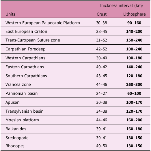
Table 2. Long description
A table comparing crustal and lithosphere thickness intervals across various tectonic units. The table has 15 rows and 3 columns. The columns are labeled ‘Units’, ‘Crust’, and ‘Lithosphere’. The ‘Crust’ and ‘Lithosphere’ columns list thickness intervals in kilometers. Row 1: Western European Palaeozoic Platform, Crust: 30-38, Lithosphere: 90-160. Row 2: East European Craton, Crust: 38-45, Lithosphere: 140-200. Row 3: Trans-European Suture zone, Crust: 31-52, Lithosphere: 150-240. Row 4: Carpathian Foredeep, Crust: 42-52, Lithosphere: 100-240. Row 5: Western Carpathians, Crust: 30-40, Lithosphere: 100-180. Row 6: Eastern Carpathians, Crust: 40-42, Lithosphere: 140-240. Row 7: Southern Carpathians, Crust: 43-45, Lithosphere: 120-180. Row 8: Vrancea zone, Crust: 44-46, Lithosphere: 260-300. Row 9: Pannonian basin, Crust: 24-27, Lithosphere: 60-100. Row 10: Apuseni, Crust: 30-38, Lithosphere: 100-170. Row 11: Transylvanian basin, Crust: 34-38, Lithosphere: 120-170. Row 12: Moesian platform, Crust: 44-46, Lithosphere: 160-200. Row 13: Balkanides, Crust: 39-41, Lithosphere: 160-180. Row 14: Srednogorie, Crust: 39-41, Lithosphere: 130-150. Row 15: Rhodopes, Crust: 40-50, Lithosphere: 130-150.
5. Discussion
5.a. Comparison with previous results
For the best possibility of comparing the LAB depths determined by us and other authors (Babuška et al. Reference Babuška, Plomerová, Šílený, Froidevaux and Fuchs1987; Horváth et al. Reference Horváth, Bada, Szafian, Tari, Adam and Cloetingh2006 and references therein; Korja, Reference Korja2007 in Jones et al. (Reference Jones, Plomerová, Korja, Sodoudi and Spakman2010); Geissler et al. Reference Geissler, Sodoudi and Kind2010; Plomerová and Babuška, Reference Plomerová and Babuška2010; Šumanovac, Reference Šumanovac2015; Alasonati Tašárová et al. Reference Alasonati Tašárová, Fullea, Bielik and Środa2016; Belinić et al. Reference Belinić, Stipčević and Živčić2018; Tiliță et al. Reference Tiliță, Lenkey, Mațenco, Horváth, Surányi and Cloetingh2018; Kalmár et al. Reference Kalmár, Petrescu, Stipčević, Balázs and János Kovács2023; Rubóczki et al. Reference Rubóczki, Novák, Liptai, Porkoláb, Molnár, Galsa, Molnár, Wesztergom and Kovács2024), three profiles A-A´, B-B´ and C-C´ were chosen in the investigated area (Figure 4). Profile A-A´ first has a NW-SE direction and then continues in WNW-ESE direction. Profile B-B´ runs N-S along the meridian 19° E, and the last profile C-C´ has an WSW-ENE direction first and then SW-NE. The selection of the profiles was influenced mainly by the fact that it was possible to compare the results of as many authors as possible (Table 3) and, at the same time, that the profiles also pass through as many tectonic units as possible. The analysis of the comparison of the results was done both quantitatively and qualitatively.
An overview of the authors and methods used to compare our and previous the LAB depth results along the profiles A-A´, B-B´ and C-C´
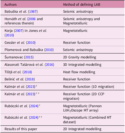
Table 3. Long description
A table with two columns and 14 rows. The first column lists authors and years, and the second column lists methods of defining LAB. Row 1: Babuška et al. (1987), Seismic anisotropy. Row 2: Horváth et al. (2006 and references therein), Seismic anisotropy and Magnetotelluric. Row 3: Korja (2007) in Jones et al. (2010), Magnetotelluric. Row 4: Gessler et al. (2010), Receiver function. Row 5: Plomerová and Babuška (2010), Seismic anisotropy. Row 6: Šumanovac (2015), 2D Gravity modelling. Row 7: Alasonati Tašárová et al. (2016), 3D Integrated modelling. Row 8: Tiliţă et al. (2018), Heat flow modelling. Row 9: Belinić et al. (2018), Receiver function. Row 10: Kalmár et al. (2023)+, Receiver function (1D migration). Row 11: Kalmár et al. (2023)++, Receiver function (2D CCP migration). Row 12: Rubóczki et al. (2024)+, Magnetotelluric (Pannon Lithosphere H2Oscope MT array). Row 13: Rubóczki et al. (2024)++, Magnetotelluric (Combined MT dataset). Row 14: Results of this paper, 2D Integrated modelling.
Profile A-A´
In the section from the Vienna Basin to the SE part of the Pannonian Basin, the LAB depths determined by different authors and methods are in relatively good agreement (Figure 5a). The thickness of the lithosphere in the Vienna Basin and the Malé Karpaty Mts. ranges from 70 km (Kalmár et al. Reference Kalmár, Petrescu, Stipčević, Balázs and János Kovács2023) to 120 km (Babuška et al. Reference Babuška, Plomerová, Šílený, Froidevaux and Fuchs1987 and Horváth et al. Reference Horváth, Bada, Szafian, Tari, Adam and Cloetingh2006). In the area of the Vienna Basin and the Malé Karpaty Mts., our results are qualitatively consistent with those of other authors. The only exceptions are the results of Kalmár et al. (Reference Kalmár, Petrescu, Stipčević, Balázs and János Kovács2023), which show smaller values of lithosphere thickness compared to ours.
Comparison of our and previous the LAB depth results (Table 3) along the profile A-A´.

The thinnest lithosphere can be observed in the Pannonian Basin. All lithosphere thickness values change from 50 km in its central part to ∼115 km in its peripheral parts. In the section of the profile at approximately 220 km (NW part of the basin) and 470 km (SE part of the basin), the largest difference between the depths of the LAB was found. The difference between the thinnest (Horváth et al. Reference Horváth, Bada, Szafian, Tari, Adam and Cloetingh2006; Korja, Reference Korja2007; Kalmár et al. Reference Kalmár, Petrescu, Stipčević, Balázs and János Kovács2023) and the thickest (Alasonati Tašárová et al. Reference Alasonati Tašárová, Fullea, Bielik and Środa2016; Rubóczki et al. Reference Rubóczki, Novák, Liptai, Porkoláb, Molnár, Galsa, Molnár, Wesztergom and Kovács2024) lithosphere here reaches more than 50 km. The lithosphere thickness determined by us ranges from 60 to 80 km and is within the range of previous results. At the NW edge of the basin, our model lithosphere is slightly thicker than the other models, but it is still within the uncertainties. Our values here reach ∼105 km.
The largest discrepancies in the estimation of the lithosphere thickness are clearly observable in the Apuseni Mts., Transylvanian Basin and Vrancea zone regions. The differences increase in the direction from the Apuseni Mts. through the Transylvanian Basin to the Vrancea zone. While in the SE part of the Apuseni Mts. (contact with Transylvanian Basin) the differences are ∼40–80 km. In the Transylvanian Basin area, the LAB of our model is 30–40 km deeper than the deepest other model (Alasonati Tašárová et al. Reference Alasonati Tašárová, Fullea, Bielik and Środa2016), while in the Vrancea zone this difference is even 60 km (model of Horváth et al. Reference Horváth, Bada, Szafian, Tari, Adam and Cloetingh2006).
In the Transylvanian Basin, it can be stated that the thinnest lithosphere (∼70–110 km) has been determined with magnetotelluric data (Korja, Reference Korja2007), seismically (Kalmár et al. Reference Kalmár, Petrescu, Stipčević, Balázs and János Kovács2023) and geothermally (Tiliță et al. Reference Tiliță, Lenkey, Mațenco, Horváth, Surányi and Cloetingh2018). In contrast, the thickest lithosphere of 170 km was determined by our integrated modelling. In Figure 5a among the mentioned values of the thinnest and thickest lithosphere, there are data determined by seismic anisotropy (Babuška et al. Reference Babuška, Plomerová, Šílený, Froidevaux and Fuchs1987; Plomerová and Babuška, Reference Plomerová and Babuška2010) and combination of magnetotelluric and seismic anisotropy methods (Horváth et al. Reference Horváth, Bada, Szafian, Tari, Adam and Cloetingh2006 and references therein). Their values drop sharply towards to the Vrancea zone, and in the southwestern-most part of the Transylvanian Basin, the lithosphere has a thickness of up ∼170 km and is approaching our results. Note that Babuška et al. (Reference Babuška, Plomerová, Šílený, Froidevaux and Fuchs1987), Horváth et al. (Reference Horváth, Bada, Szafian, Tari, Adam and Cloetingh2006) and our results show probably the least agreement with the P-wave low velocity anomaly, which was interpreted in the SE part of the Transylvanian Basin by Martin et al. (Reference Martin and Wenzel2006). Its centre was estimated at a depth of only about 80–100 km. A partial explanation for this discrepancy can be found in the fact that our input values of surface heat flow in this basin have not been corrected for paleoclimate, thickness of sediments and erosion, as was done in the geothermal modelling of Tiliță et al. (Reference Tiliță, Lenkey, Mațenco, Horváth, Surányi and Cloetingh2018). Since the temperatures are not yet in equilibrium, this region is certainly not in local equilibrium, which was also stated by Tilita et al. (Reference Tiliţă, Matenco, Dinu, Ionescu and Cloetingh2013, Reference Tiliță, Lenkey, Mațenco, Horváth, Surányi and Cloetingh2018) and Balazs et al. (Reference Balázs, Faccenna, Gerya, Ueda and Funiciello2022). Our modelling was performed under the condition of local isostasy, which may not be the case for Transylvanian Basin and Vrancea zone and under steady-state thermal conditions. For Transylvanian Basin, this was indicated, for example, by Balling et al. (Reference Balling, Grützner, Tomljenović, Spakman and Ustaszewski2022) and Kalmár and Balázs (Reference Kalmár, Petrescu, Hetényi, Michailos, Süle, Neagoe and Bokelmann2025). As said earlier, in this case, our model gives a maximum possible depth, and the real depth may thus be significantly smaller. However, a difference of nearly 100 km is more than can be expected. Therefore, we think that the real depth of the thermal LAB may be somewhere between the seismically defined depth and one of our models.
In the Transylvanian Basin and Vrancea zone contact area, our results indicate that the thickness of the lithosphere increases steeply up to a depth of 300 km. The vertical change was also qualitatively noted by Horváth et al. (Reference Horváth, Bada, Szafian, Tari, Adam and Cloetingh2006). The near-vertical decrease of the 1300°C isotherm interpreted by heat flow modelling (Tiliță et al. Reference Tiliță, Lenkey, Mațenco, Horváth, Surányi and Cloetingh2018) supports our results, although these authors place the vertical step approximately 30 km to the west.
In the Vrancea zone, the maximum lithosphere thickness modelled by us reaches the already mentioned 300 km. This value is 240 km according to Horváth et al. (Reference Horváth, Bada, Szafian, Tari, Adam and Cloetingh2006), 180 km after Babuška et al. (Reference Babuška, Plomerová, Šílený, Froidevaux and Fuchs1987) and Plomerová and Babuška (Reference Plomerová and Babuška2010) and ∼190 km by Geissler et al. (Reference Geissler, Sodoudi and Kind2010). Interestingly, the location of the LAB in Vrancea zone estimated by Korja (Reference Korja2007) and Kalmár et al. (Reference Kalmár, Petrescu, Stipčević, Balázs and János Kovács2023) shows only a slight change in lithosphere thickness compared to the thickness determined in adjacent Transylvanian Basin and does not reflect the pronounced high velocity anomaly discovered by 3D seismic tomography (Wortel and Spakman, Reference Wortel and Spakman2000; Martin et al. Reference Martin and Wenzel2006). According to these authors, the LAB depths reach only ∼110–130 km. Even though our modelled lithospheric thickness cannot reflect the subducted slab itself, only the thickening of the lithosphere, it seems that our location of the LAB is in the best agreement with the high-velocity anomaly.
Profile B-B´
Comparison of the results along the profile B-B´ (Figure 5b) shows that the LAB depth values in the Trans-European Suture Zone, West European Palaeozoic Platform and Carpathian Foredeep units, determined by all authors are in good agreement and range from ∼140 to ∼180 km with the only exception of Kalmár’s et al. (Reference Kalmár, Petrescu, Stipčević, Balázs and János Kovács2023) model, which is up to 80 km shallower compared to our model.
Comparison of our and previous the LAB depth results (Table 3) along the profile B-B´.

Figure 5b. Long description
Panel: A line graph titled Profile B-B’. The horizontal axis represents distance in kilometers ranging from 0 to 800 kilometers. The vertical axis represents depth in kilometers ranging from 0 to 260 kilometers. The graph includes multiple lines representing different studies and their results. The lines are labeled with the names of the studies and the years they were conducted. The trends of the lines show variations in the depth of the lithosphere-asthenosphere boundary across the distance. The labels at the top of the graph indicate different geological features and regions along the profile.
In the areas of the External Carpathians Flysch Belt and internal parts of the Western Carpathians, our LAB has a constant depth of ∼180 km, much deeper than in other models. The smallest values of ∼70–100 km were obtained by Kalmár et al. (Reference Kalmár, Petrescu, Stipčević, Balázs and János Kovács2023). Between the Trans-European Suture Zone and the Pannonian Basin, all authors indicate a similar thinning, however, in the other models, this thinning occurs gradually between the External Carpathians Flysch Belt and the Pannonian Basin, whereas in our model, there is a steep thinning within the Western Carpathians.
The best agreement of all compared results is observed in the central part of the Pannonian Basin, where in the profile section from 400 to 550 km, the lithosphere thickness ranges from 60 to 80 km. In the southwestern part of the Pannonian Basin towards the Southern Carpathians, the thickness of the lithosphere increases again in a gradual way. However, according to different authors, the onset of lithosphere thickening is different. In the case of Horváth et al. (Reference Horváth, Bada, Szafian, Tari, Adam and Cloetingh2006), Plomerová and Babuška (Reference Plomerová and Babuška2010) and Kalmár et al. (Reference Kalmár, Petrescu, Stipčević, Balázs and János Kovács2023), this onset starts at a profile distance of 600 km, whereas in the case of Babuška et al. (Reference Babuška, Plomerová, Šílený, Froidevaux and Fuchs1987), it is about 100 km earlier. The depths of the LAB in the Southern Carpathians after Horváth et al. (Reference Horváth, Bada, Szafian, Tari, Adam and Cloetingh2006), Plomerová and Babuška (Reference Plomerová and Babuška2010) and Kalmár et al. (Reference Kalmár, Petrescu, Stipčević, Balázs and János Kovács2023) ranges from ∼75 km to ∼120 km.
Profile C-C´
Based on our and Šumanovac (Reference Šumanovac2015) and Belinič et al. (Reference Belinić, Stipčević and Živčić2018) results, we observed very thin lithosphere in the Pannonian Basin and, conversely, a relatively thick lithosphere under the Dinarides (Figure 5c). The agreement of the LAB depth in the Pannonian Basin is very good. According to all authors, it ranges from 60 km in the centre to ∼95 km in the W where the lithosphere thickens towards the Dinarides. Although the exact position of the LAB under the Dinarides differs between the models, the values of the maximum lithosphere thickness are quite similar. According to Šumanovac (Reference Šumanovac2015), it is 175 km, 150 km after Belinovič et al. (Reference Belinić, Stipčević and Živčić2018), and according to our results, it is 160 km. Towards the SW, the depths of the LAB begin to diverge in the interval from 110 km (Belinič et al. Reference Belinić, Stipčević and Živčić2018) to ∼155 km (our modelling). It may be partly caused by the fact that our calculations were made under the assumption of the validity of local isostasy, which may not apply in the Dinarides (Balling et al. Reference Balling, Grützner, Tomljenović, Spakman and Ustaszewski2022). Note that Šumanovac (Reference Šumanovac2015) determined the thickness based on 2D gravity modelling. It is known that this method, unless seismic data are available, shows a high degree of uncertainty in defining the LAB depth. For completeness, it is necessary to add that the existence of a lithosphere slab under the Dinarides was investigated using teleseismic tomography (Šumanovac and Dudjak, Reference Šumanovac and Dudjak2016; Šumanovac et al. Reference Šumanovac, Markušić, Engelsfeld, Jurković and Orešković2017) and seismic modelling (Šumanovac, Reference Šumanovac2022). Based on these results, structural models were developed in the northern and southern Dinarides. Given the fact that these studies did not provide a lithosphere thickness map, we could not perform a quantitative comparison.
Comparison of our and previous the LAB depth results (Table 3) along the profile C-C´.

At the end of this part, we state that the differences in the LAB depths determined by all authors are significant in some tectonic units. In relation to this statement, we fully agree with the conclusions of Jones et al. (Reference Jones, Plomerová, Korja, Sodoudi and Spakman2010), who say: ‘These differences are not random. Each LAB data in different domains can reflect some aspects of the physical transition from the lithosphere to the asthenosphere, which need not be the same for different parameters, for different ages of the provinces, and of the same intensity relative to other discontinuities in the upper mantle’. Based on our results, we can expand their idea that LAB data can also reflect different geodynamic development of the lithosphere.
Our ambition when comparing the LAB depths was not to determine which of the methods used is worse or better. On the contrary, we wanted to contribute to solving this problem. The results clearly show that in the future, many open questions remain in LAB research.
5.b. Tectonic implications
Our modelling shows clearly significant variations in the LAB depths along the strike of the Carpathian orogen (Figure 4). The increase of the lithospheric thickness from the Western Carpathians to the Eastern Carpathians supports the suggestion that the slab break-off began in the Western Carpathians and spread along the arc toward the SE up to the Vrancea zone, where the slab break-off has not yet occurred (e.g., Martin et al. Reference Martin and Wenzel2006). This zone is regarded as the ultimate expression of the progressive subduction, slab roll-back and plate boundary retreat that were responsible for the evolution of the Carpathian arc (Lillie et al. Reference Lillie, Bielik, Babuška and Plomerová1994; Tomek and PANCARDI colleagues, Reference Tomek, Gee and Zeyen1996; Nemčok et al. Reference Nemčok, Pospíšil, Lexa and Donelick1998; Sperner et al. 2001, Reference Sperner, Ioane and Lillie2004; Kázmér et al. Reference Kázmér, Dunkl, Frisch, Kuhlemann and Ozsvárt2003; Kalmár et al. Reference Kalmár, Petrescu, Hetényi, Michailos, Süle, Neagoe and Bokelmann2025). The subduction process had been accompanied by roll-back and slab detachment (Linzer, Reference Linzer1996; Wortel and Spakman, Reference Wortel and Spakman2000; Sperner et al. Reference Sperner, Lorenz, Bonjer, Hettel, Müller and Wenzel2001, Reference Sperner, Ratschbacher and Nemčok2002). According to Wortel and Spakman (Reference Wortel and Spakman2000), the lower part of the broken slab gradually sunk into the deeper mantle and formed a distinct horizontal P-wave velocity anomaly at depths from 410 to 660 km beneath the Pannonian Basin System. The newest study of the mantle transition zone by seismic tomography and receiver functions analyses (Kalmár et al. Reference Kalmár, Petrescu, Hetényi, Michailos, Süle, Neagoe and Bokelmann2025) support this ‘slab graveyard’ hypothesis. The accumulated subducted slabs reside predominantly in the lower mantle transition zone, marked by a depressed seismic discontinuity at 660 km depth.
Modelling results show that the lithosphere thickening in the Eastern Carpathians, especially in the Vrancea zone, can be interpreted as the remnant of a subducted plate. Remnants of deep subduction and slab detachment below the Carpathian-Pannonian Basin region have been detected by 3-D seismic tomography (Spakman, Reference Spakman1990; Spakman et al. Reference Spakman, van der Lee and van der Hilst1993; Goes et al. Reference Goes, Spakman and Bijwaard1999; Wortel and Spakman, Reference Wortel and Spakman2000; Martin et al. Reference Martin, Achauer, Kissling, Mocanu, Musacchio, Radulian and Wenzel2001, Reference Martin and Wenzel2006). Based on these results, it can be concluded that the increasing thickness of the lithosphere eastward along the direction of the Carpathian orogen reflects the lateral migration of the plate detachment along the plate boundary. We assume that lithospheric thickening along the Eastern Carpathians is the result of a gradual sinking of the upper part of the broken slab during continuing convergence between the Eurasian plate and ALCAPA and Tisza-Dacia microplates, which is here characterized by frontal continental collision (Bielik et al. Reference Bielik, Zeyen, Starostenko, Makarenko, Legostaeva, Savchenko, Dérerová, Grinč, Godová and Pánisová2022). Based on our results the largest lithosphere thickening (the lithospheric root) is observed in the Vrancea zone (∼300 km). After Martin et al. (Reference Martin and Wenzel2006) the high-velocity Vrancea body reaches a maximum depth of about 350–370 km.
Unlike the easternmost segment of the Western Carpathians and the Eastern Carpathians (including the Vrancea zone), no lithospheric thickening is observed in the western segment of the Carpathians (Figure 4). The differences could be explained by the different geodynamic evolution of these areas. After Ratschbacher et al. (Reference Ratschbacher, Frisch, Linzer and Merle1991a, Reference Ratschbacher, Merle, Ph and Cobboldb), Fodor et al. (Reference Fodor, Csontos, Bada, Györfi, Benkovics, Durand, Jolivet, Horváth and Séranne1999), Lankreijer et al. (Reference Lankreijer, Bielik, Cloetingh and Majcin1999) and Kováč (Reference Kováč2000), the ALCAPA microplate escaped in the Miocene from the Alpine collision zone towards the NE into the open ‘Carpathian Bay’. The escape and displacement of ALCAPA were caused by the Bohemian Massif blocking convergence in the colliding Alpine region (Lankreijer et al. Reference Lankreijer, Bielik, Cloetingh and Majcin1999). Since the subsequent movement of the ALCAPA microplate along the eastern margin of the Bohemian Massif was mainly left-lateral oblique collision, no thickening of the lithosphere occurred in the western part of the Western Carpathians.
The type of plate (oceanic versus continental) that is currently subducting or breaking beneath the Vrancea Zone remains a subject of scientific debate. There are alternative explanations of the oceanic slab subduction and progressive lateral tear within the Carpathian foreland. For example, Knapp et al. (Reference Knapp, Knapp, Raileanu, Matenco, Mocanu and Dinu2005) and Fillerup et al. (Reference Fillerup, Knapp, Knapp and Raileanu2010) provided an alternative model for this zone, which assumes active continental lithospheric delamination, resulting from the Miocene closure of an intra-continental basin and attendant lithospheric thickening. Bokelmann and Rodler (Reference Bokelmann and Rodler2014) do not agree with this conclusion. They suggest that the seismic anomaly under the Vrancea region represents a subducted oceanic lithosphere rather than continental lithosphere at depths shallower than the seismically active zone.
Another model invoking gravitational instability (lithospheric dripping) was presented by Gemmer and Houseman (Reference Gemmer and Houseman2007) and Houseman and Gemmer (Reference Houseman and Gemmer2007). This model offers a dynamically self-consistent explanation for the occurrence of lithospheric extension and regional subsidence in the Pannonian Basin while convergence and crustal thickening occurred beneath the surrounding Carpathians. Downwelling of the lithosphere beneath the Carpathians appears to have progressively migrated south-eastward along the Eastern Carpathians, culminating in the present day with intense seismic activity beneath the Vrancea region.
The analysis of LAB depth comparisons in the Transylvanian Basin showed significant differences. There, seismic models (e.g., Tiliță et al. Reference Tiliţă, Matenco, Dinu, Ionescu and Cloetingh2013 or Kalmár et al. Reference Kalmár, Petrescu, Stipčević, Balázs and János Kovács2023) and numerical models (e.g., Balazs et al. Reference Balázs, Faccenna, Gerya, Ueda and Funiciello2022 or Tiliță et al. Reference Tiliță, Lenkey, Mațenco, Horváth, Surányi and Cloetingh2018) based on the seismic models and surface heat flow gave LAB depths at only 85–100 km despite the relatively low surface heat flow. These authors interpret the Transylvanian Basin as due to recent slab break-off with ongoing adjustment of topography (strong uplift). According to them, it is likely that in this region, the lithosphere has been recently thinned, starting in Pliocene times, by the upwelling part of the asthenospheric circuit driven by the sinking of the Vrancea slab, as demonstrated by multiple geophysical studies (Ismail-Zadeh et al. Reference Ismail-Zadeh, Matenco, Radulian, Cloetingh and Panza2012 and references therein, Petrescu et al. Reference Petrescu, Stuart, Houseman and Bastow2020). Similarly, the tectonic mechanism driving the regional Middle-Upper Miocene subsidence of the Transylvanian Basin does not have an imprint in the recent crustal thermal field due to the large time constant of the lithosphere.
Our results clearly show evidence for the underthrusting of the Moesian Platform beneath the Southern Carpathians. This could be the result of the clockwise rotation (dextral wrenching in the sense of Matenco, Reference Matenco1997) of the lighter and younger TISZA-DACIA microplate against the denser, older and static Moesian Platform during the Neogene. According to Schleder et al. (Reference Schleder, Lăpădat, Trandafir, Fernández, Tămaș, Tămaș, Filipescu, Krézsek, Rădoiaș and Vasiliu2023), this collision also resulted in the formation of the Getic Depression, which is located south of the Southern Carpathians. This foredeep depocentre, reaching depths of up to 10 km, developed in an oblique convergent regime from the Late Cretaceous to the Paleogene, with subsequent shortening occurring during the Badenian until the present period. These results are supported by the existence of the large gravity low along the Southern Carpathians (Bielik et al. Reference Bielik, Grabowska, Bojdys, Csicsay, Šefara and Speváková2006), which can be explained by the summation of the gravity effects of the thick foredeep sediments and the crustal root beneath this mountain range (Bielik et al. Reference Bielik, Zeyen, Starostenko, Makarenko, Legostaeva, Savchenko, Dérerová, Grinč, Godová and Pánisová2022). The southern part of the Moesian Platform is underthrust beneath the Balkanides and Rhodopes, which is in good accordance with previous studies (e.g., Nakov, Reference Nakov2008; Schmid et al. Reference Schmid, Bernoulli, Fügenschuh, Matenco, Schefer, Schuster, Tischler and Ustaszewski2008).
6. Conclusions
We present a summary of more than 20 years of work on lithospheric structure using joint modelling, which was initially pushed by EUROPROBE and David Gee’s initiative.
Joint modelling of surface heat flow, gravity, geoid and topographic data, using state-of-the-art geological, seismic and other geophysical data as constraints, allowed us to establish a model of the lithospheric structure of the Carpathian-Pannonian region and its surrounding tectonic units and to present a new, original map of the LAB depth.
Underneath the Carpathian orogen, the thickness of the lithosphere shows important variations across the chain as well as along-strike. Across the Carpathian chain, the lithospheric thickness increases in the direction from the younger and warmer Pannonian Basin to the older and colder East European Craton and platforms, being modified by recent and ongoing tectonic processes. The lithospheric thickness increases from the internal (∼100–160 km) to the external (up to 220 km) parts of the Carpathian orogen. Along-strike the Carpathians, the lithosphere thickness increases from the Western Carpathians to the Eastern Carpathians. Under the westernmost segment of the Western Carpathians, no lithospheric thickening is observed, with the values in the range of 100 to 120 km. The ‘normal’ lithosphere thickness can be explained by oblique collision since the movement of the lithospheric plates was mainly strike-slip along a deep-reaching fault following the contact of the Bohemian Massif and the Western Carpathians. The beginning of the lithosphere thickening (up to 160–180 km) can be observed in the eastern segment of the Western Carpathians and continues along the Eastern Carpathians, where, in the Ukrainian and Romanian part of the Carpathian Foredeep, the thickness of the lithosphere reaches values of about 240 km. The largest lithospheric thickness (300 km) is observed in the Vrancea zone. This thickening is likely induced by remnants of a slab, the break-off of which started in the Miocene.
Our results clearly show that changes in lithosphere thickness are influenced not only by the age of tectonic units but also by geodynamic processes occurring within them.
Acknowledgements
We dedicate the paper to the memory of our excellent geologist, colleague and friend David Gee. It was he who was one of the first to stand at the forefront of cooperation between geoscientists of western and eastern Europe within the framework of the important international EUROPROBE project. In many congresses and workshops, he brought together researchers from different fields in geosciences with different backgrounds. We thank to the three reviewers and Randell Stephenson for their constructive comments on the first version of the paper and V. Hurai for helping to solve petrological problems. MB acknowledges the Slovak Research and Development Agency under the contracts Nos. APVV-21-0159, APVV-24-0445 and the VEGA Slovak Grant Agency under projects no. 2/0002/23 and no. 1/0107/23. JD acknowledges the VEGA Slovak Grant Agency under project No. 2/0013/25. The study was also investigated in the frameworks of the ILP (CoLiBrI) and AdriaArray projects.
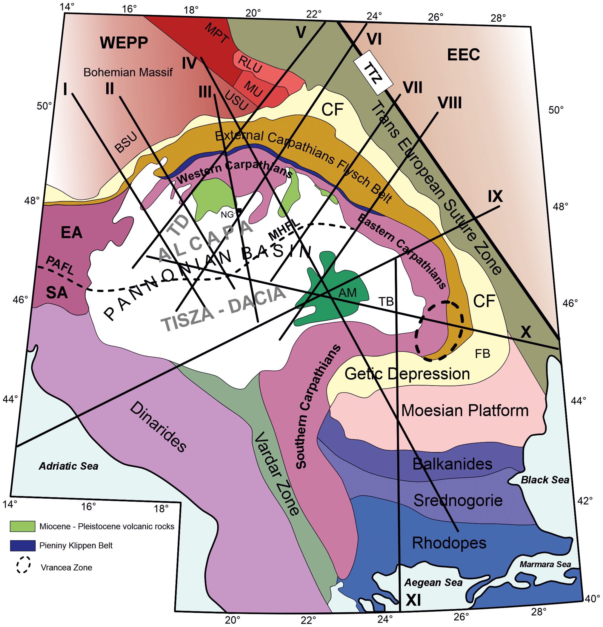
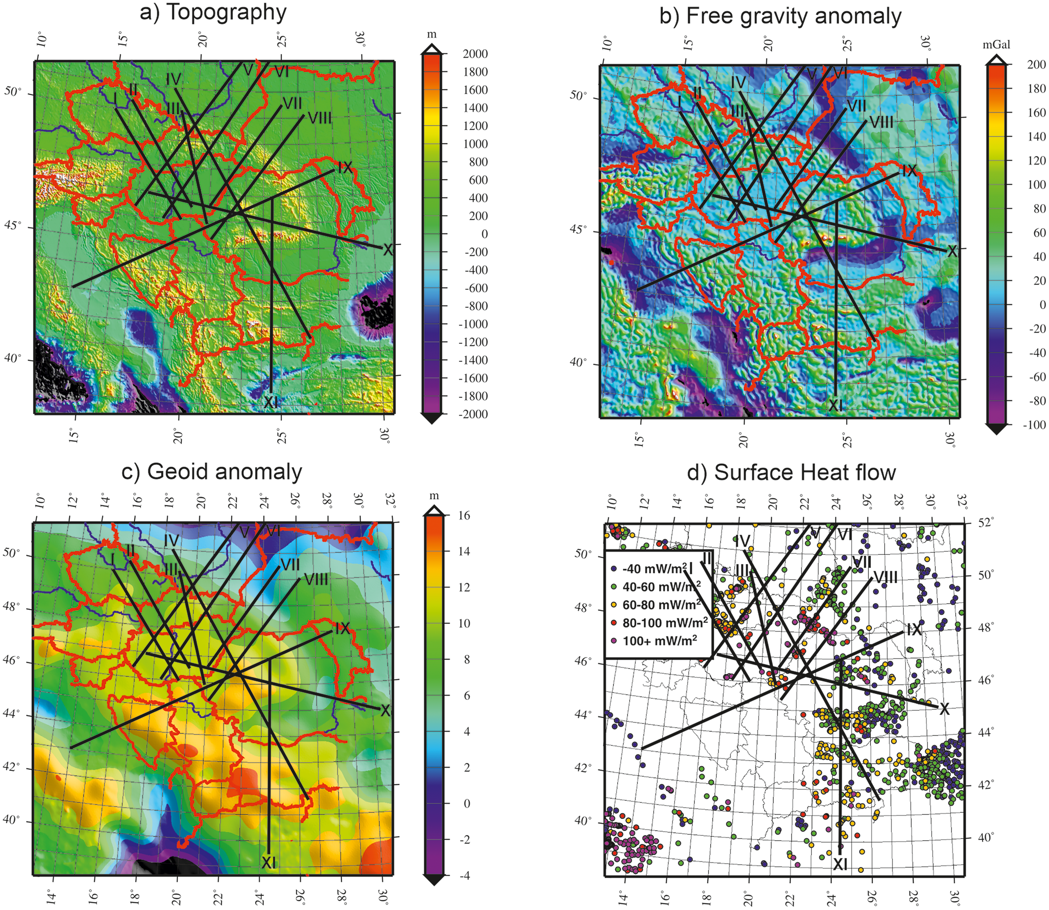
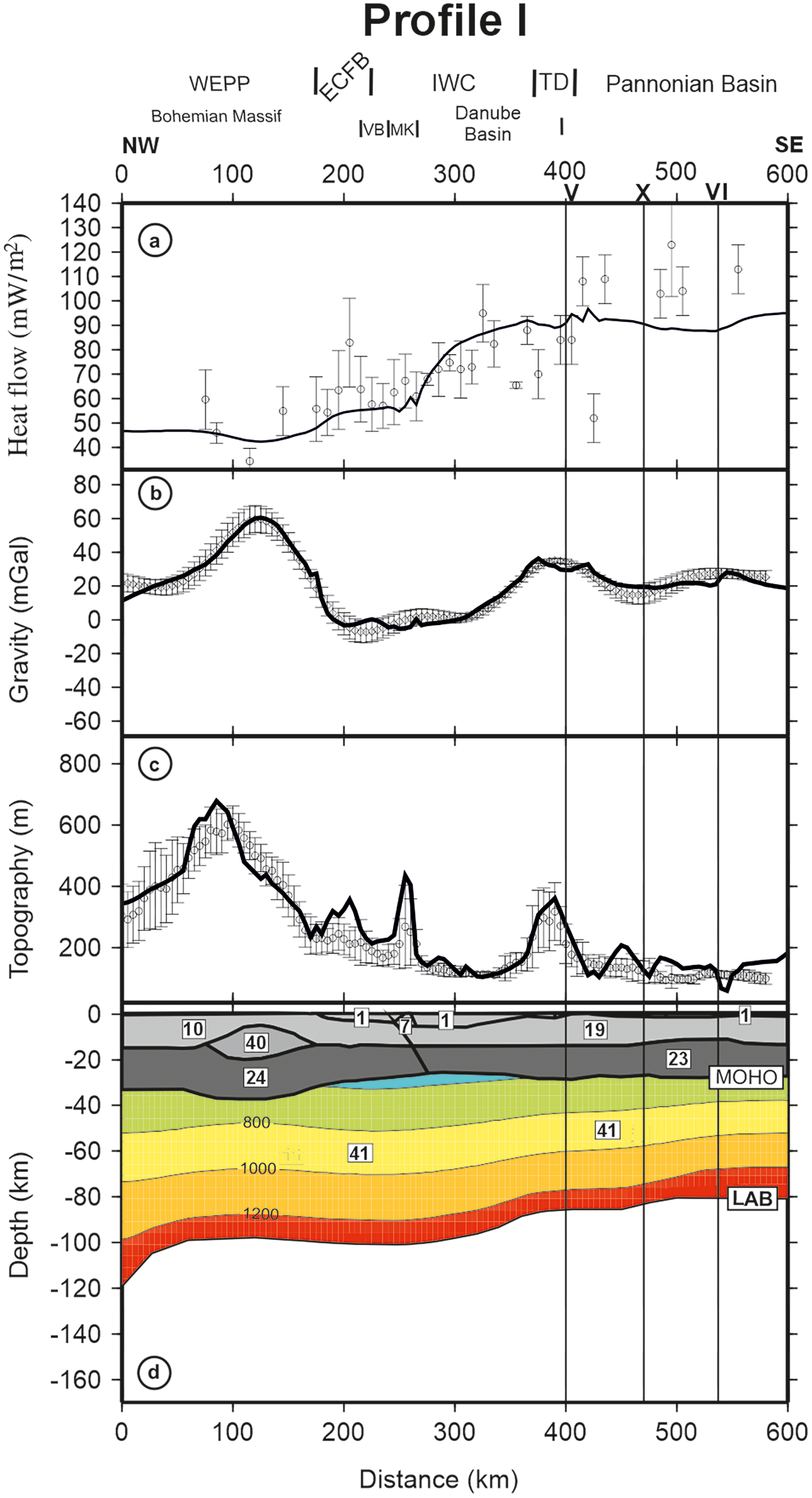
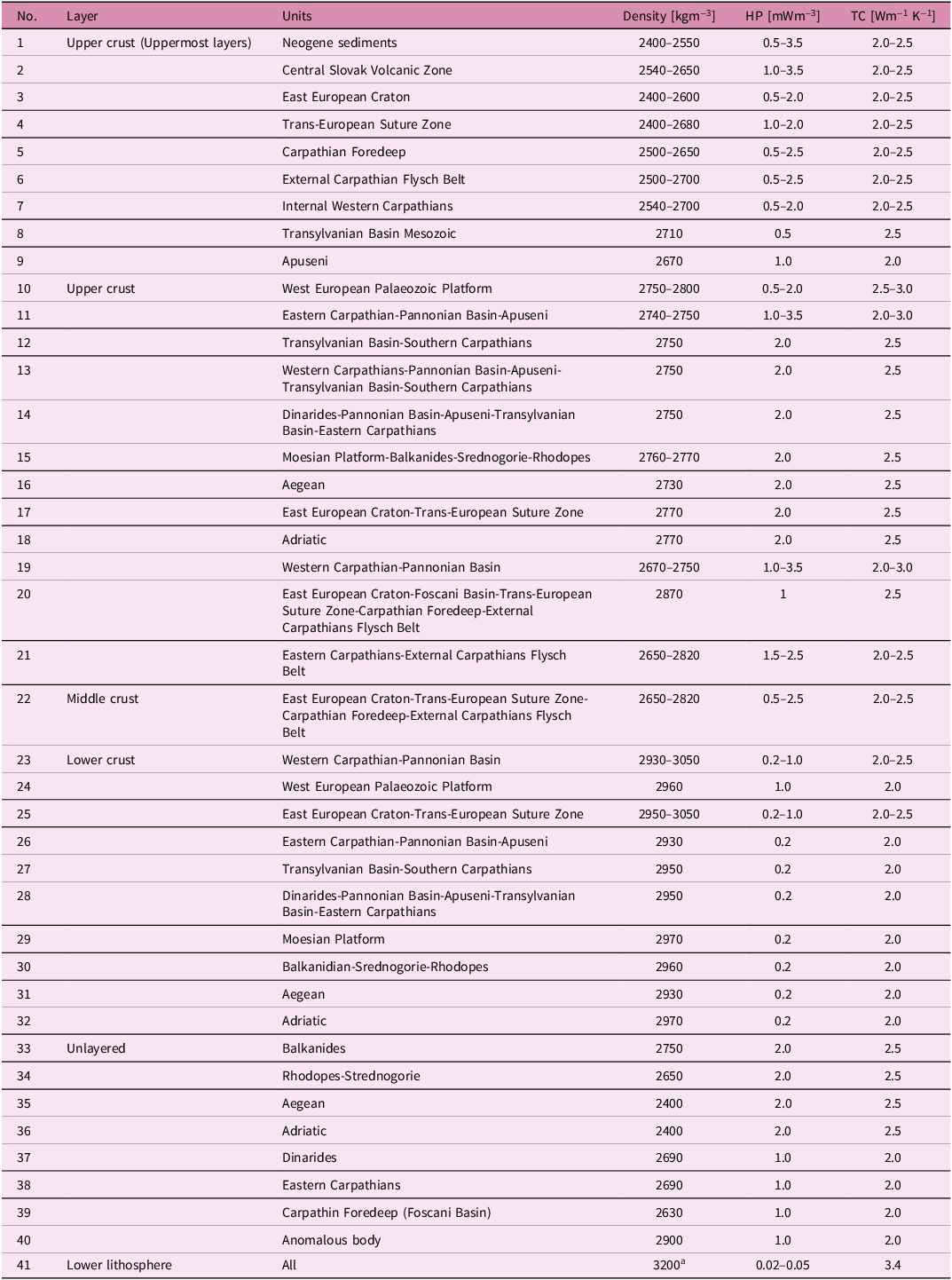
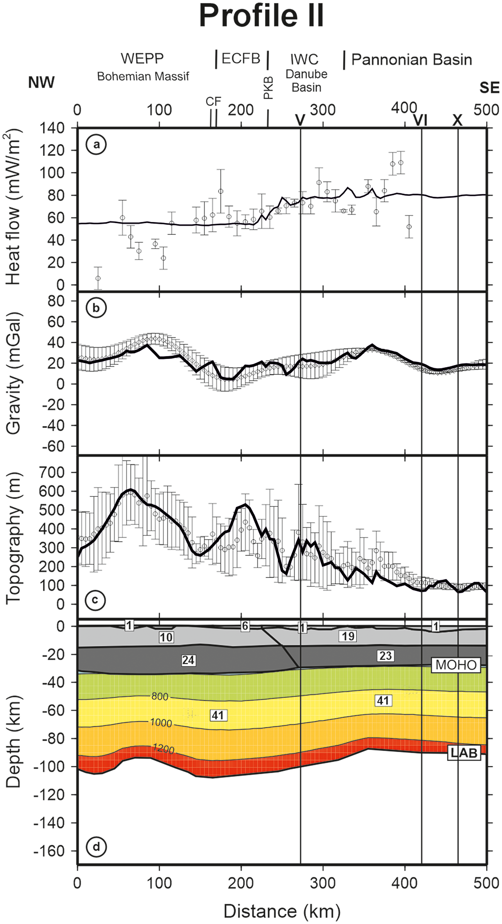
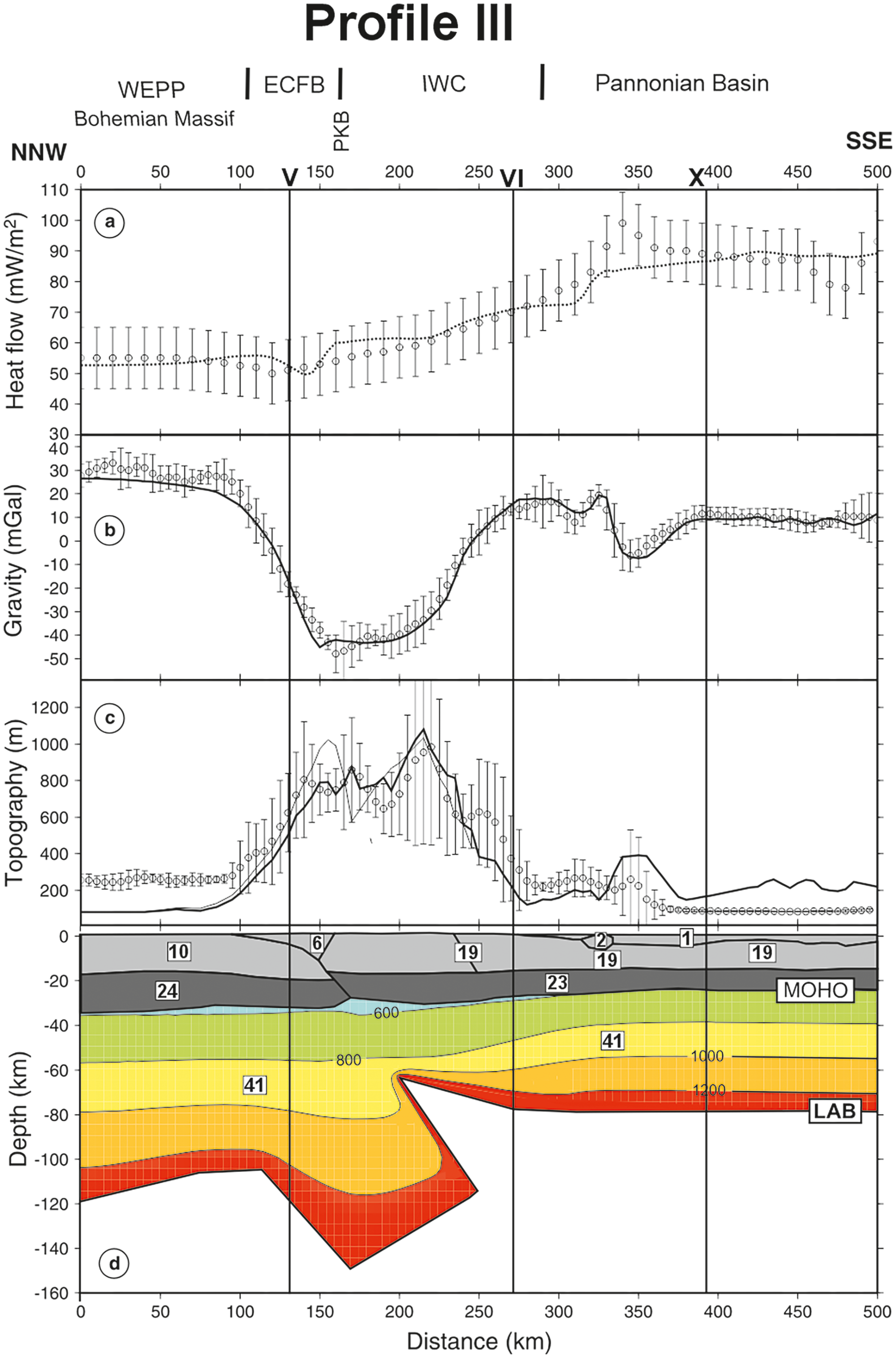
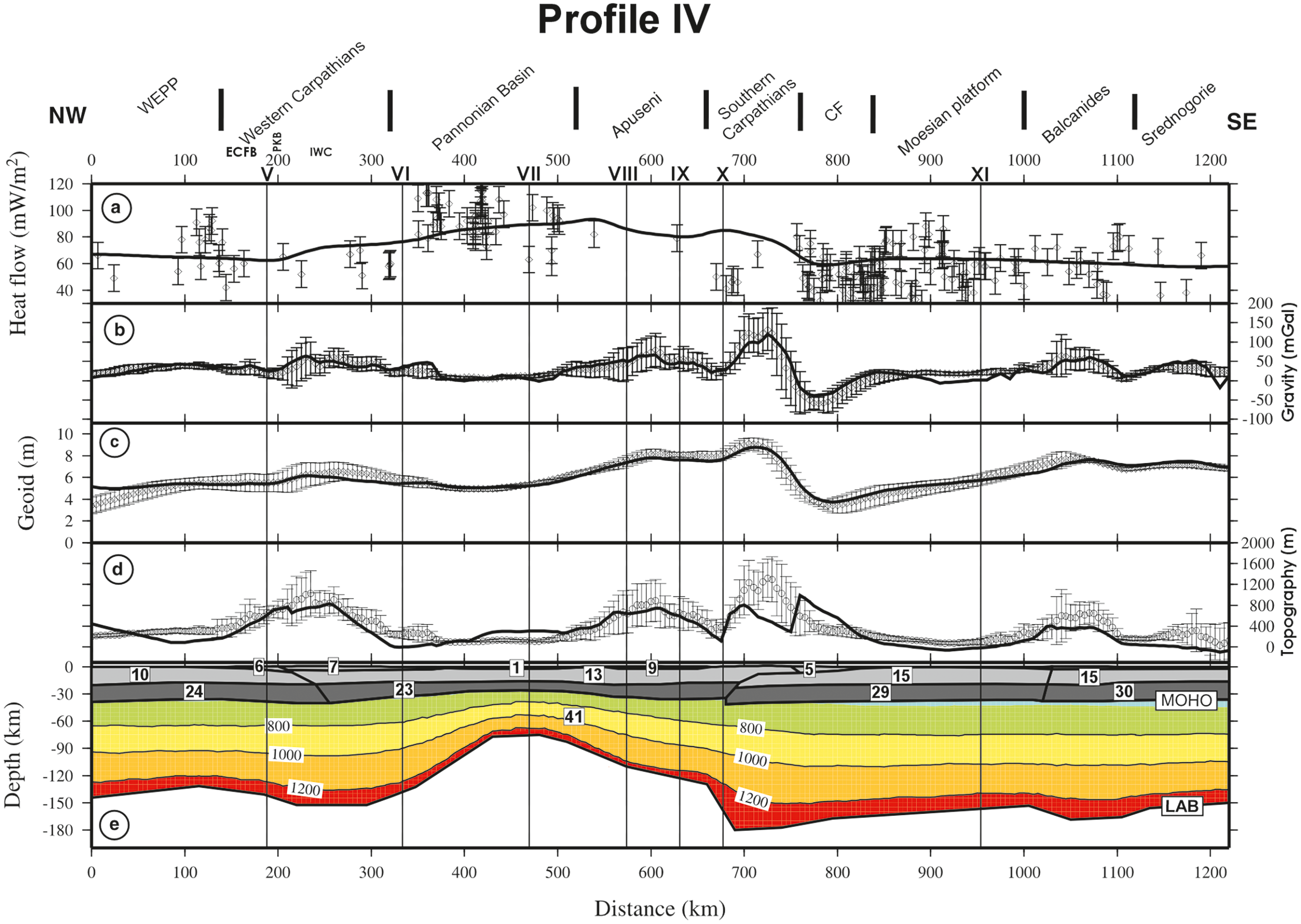
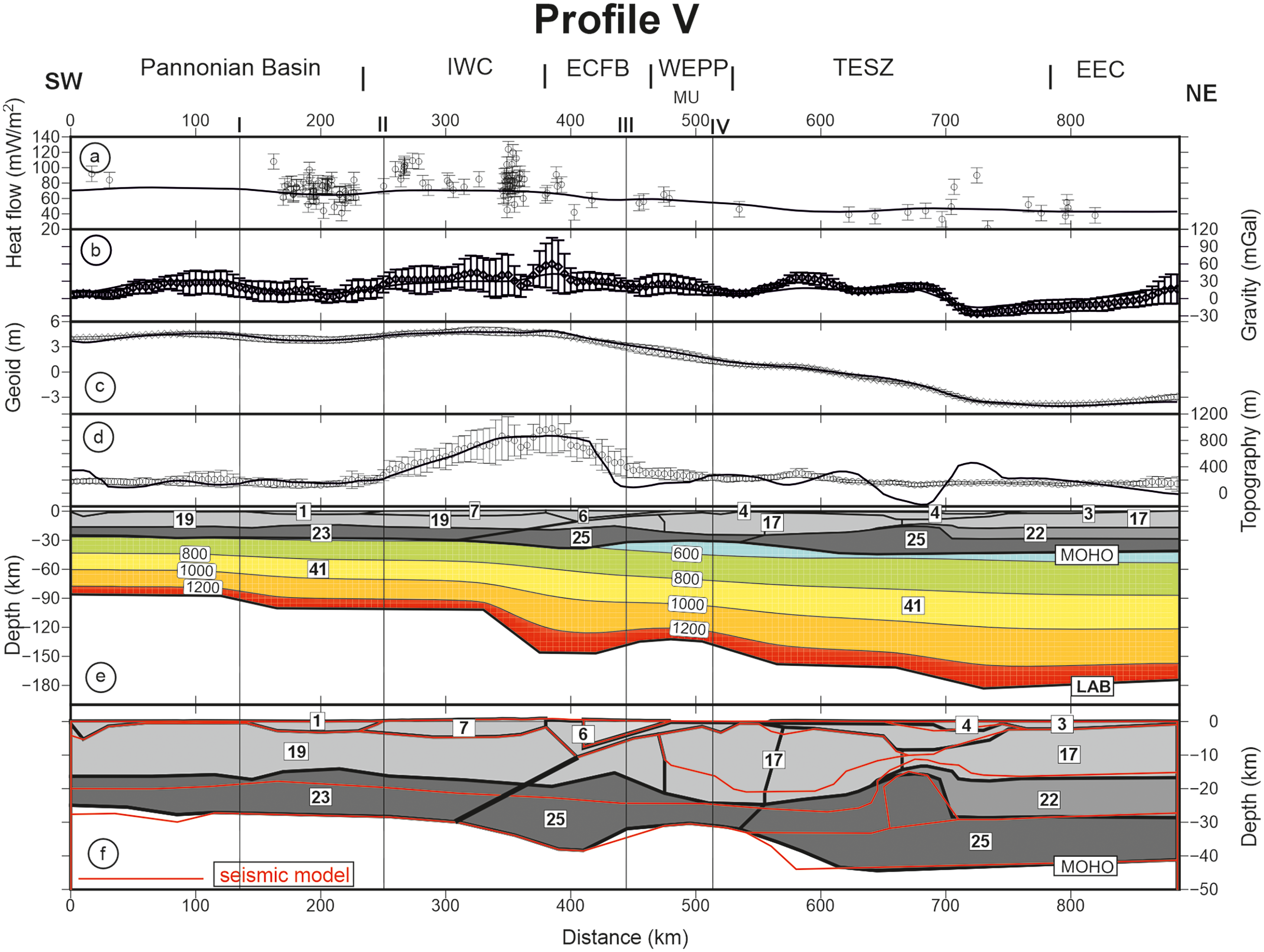
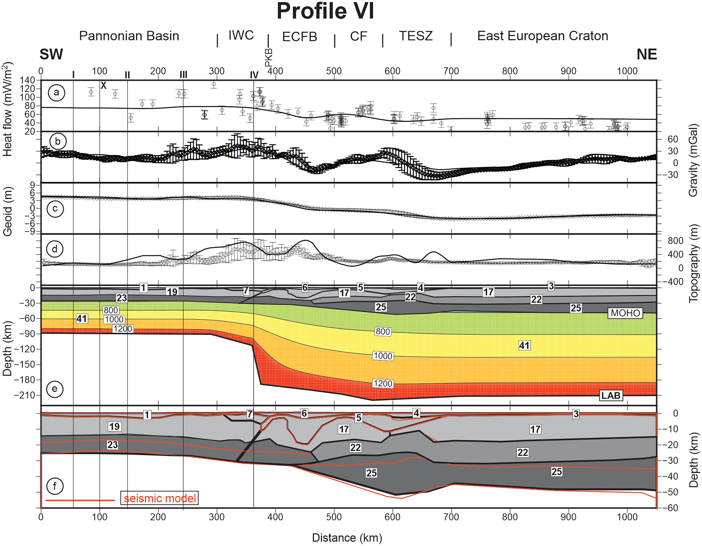
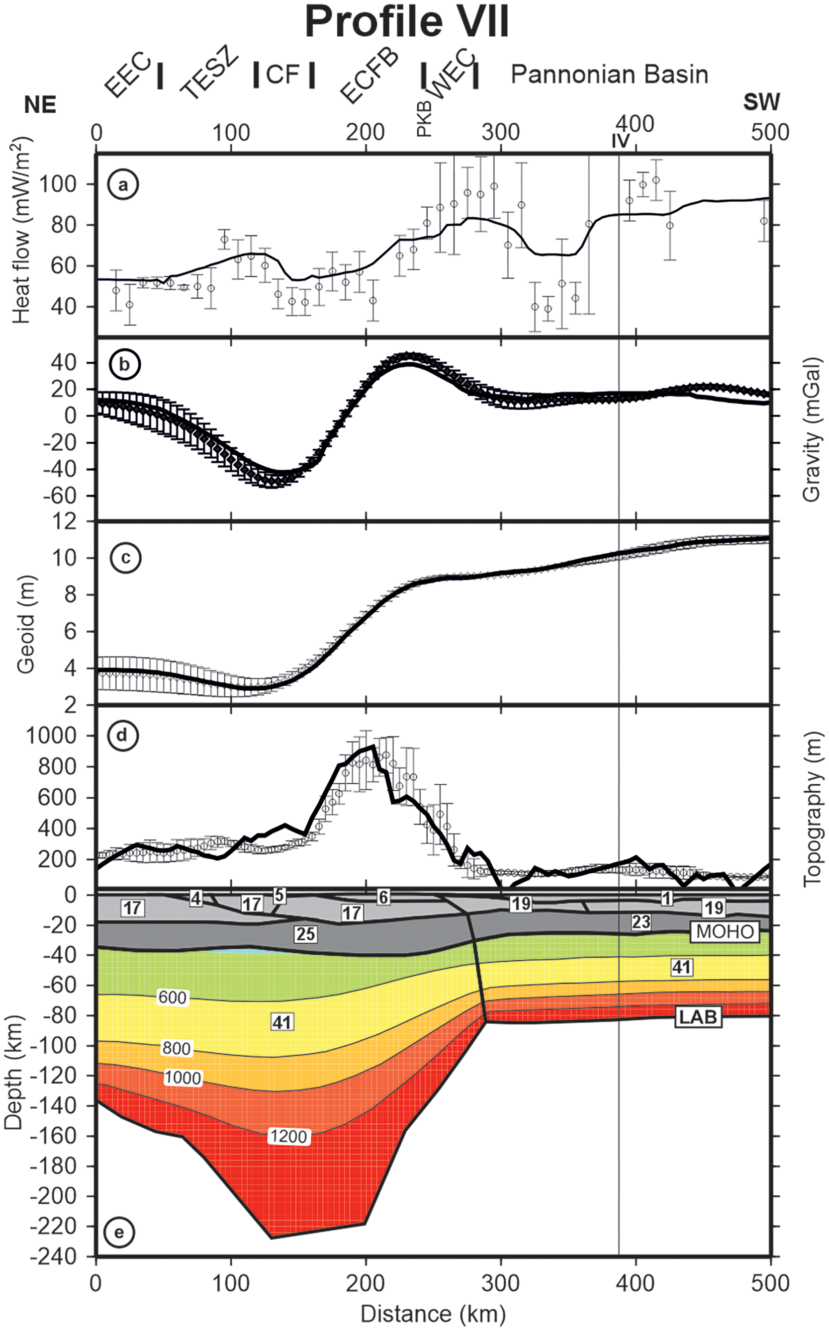
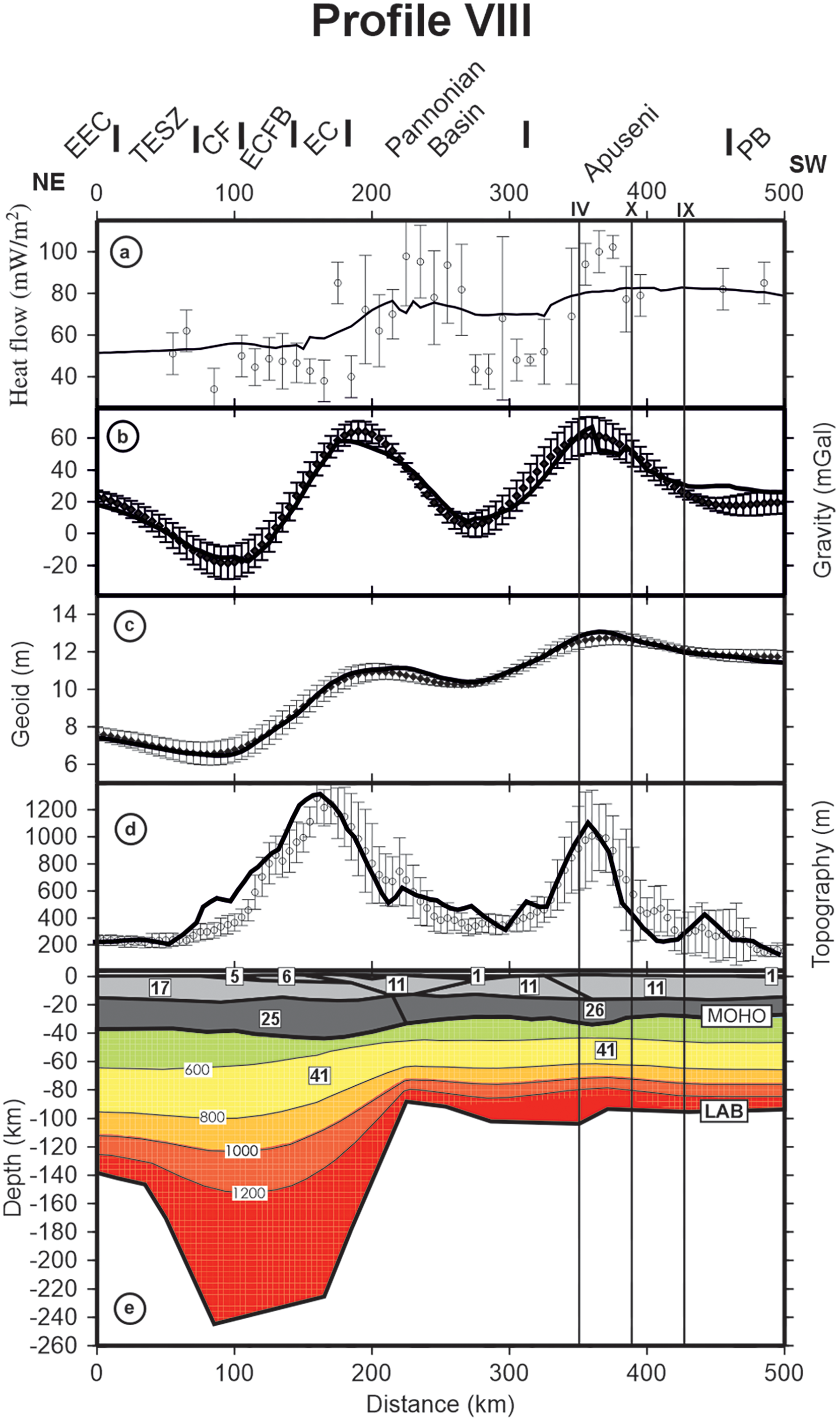
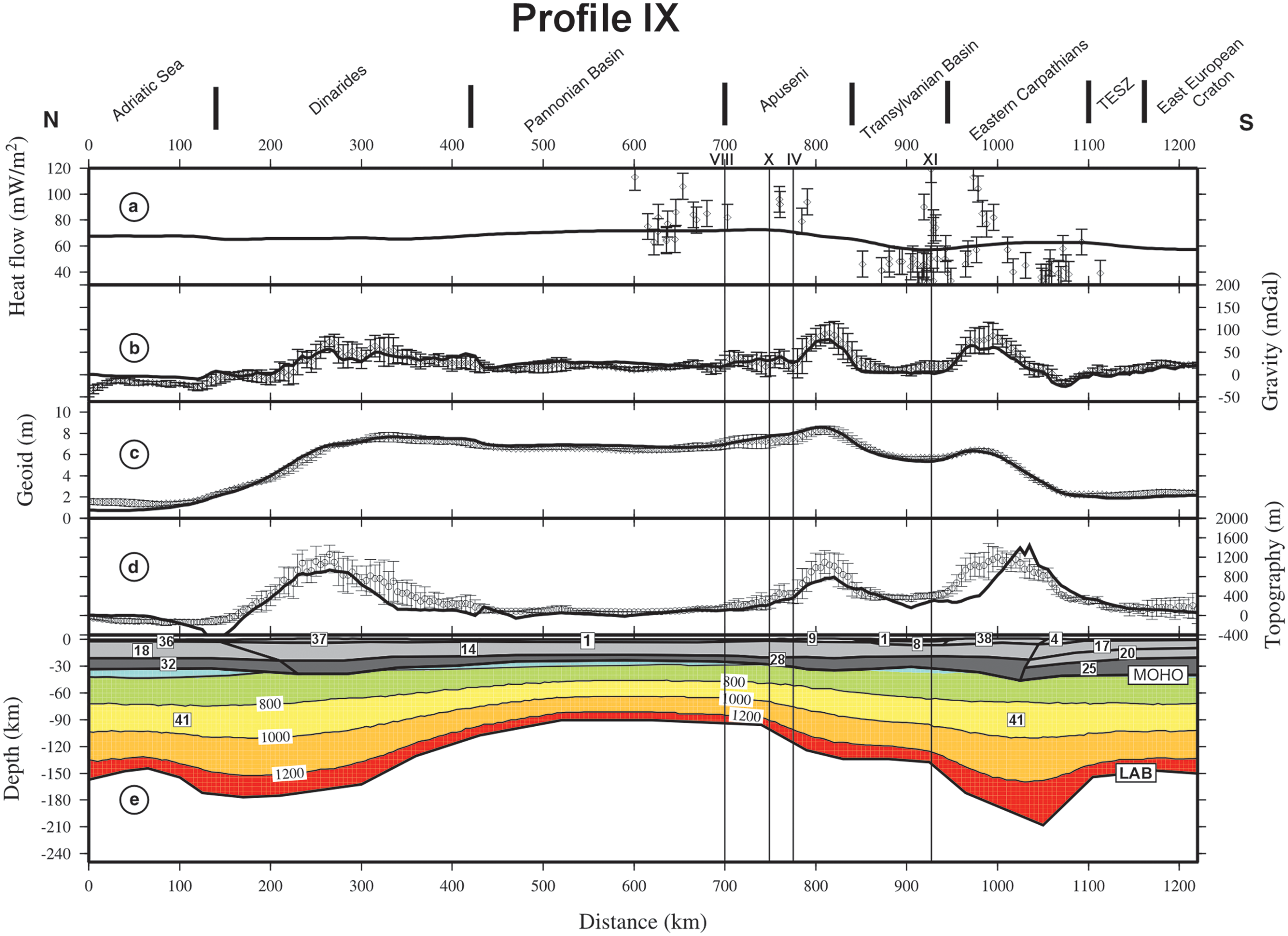
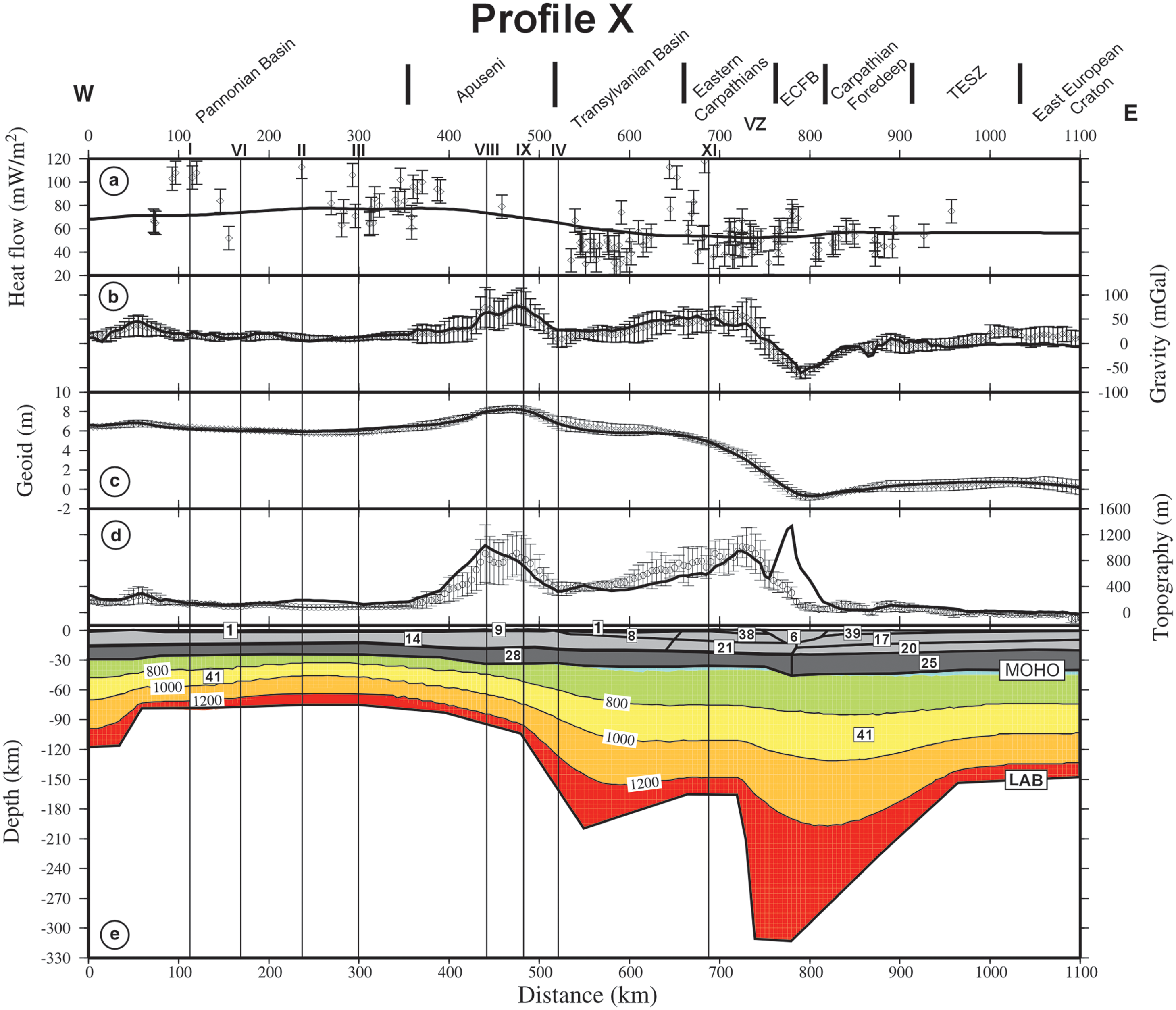
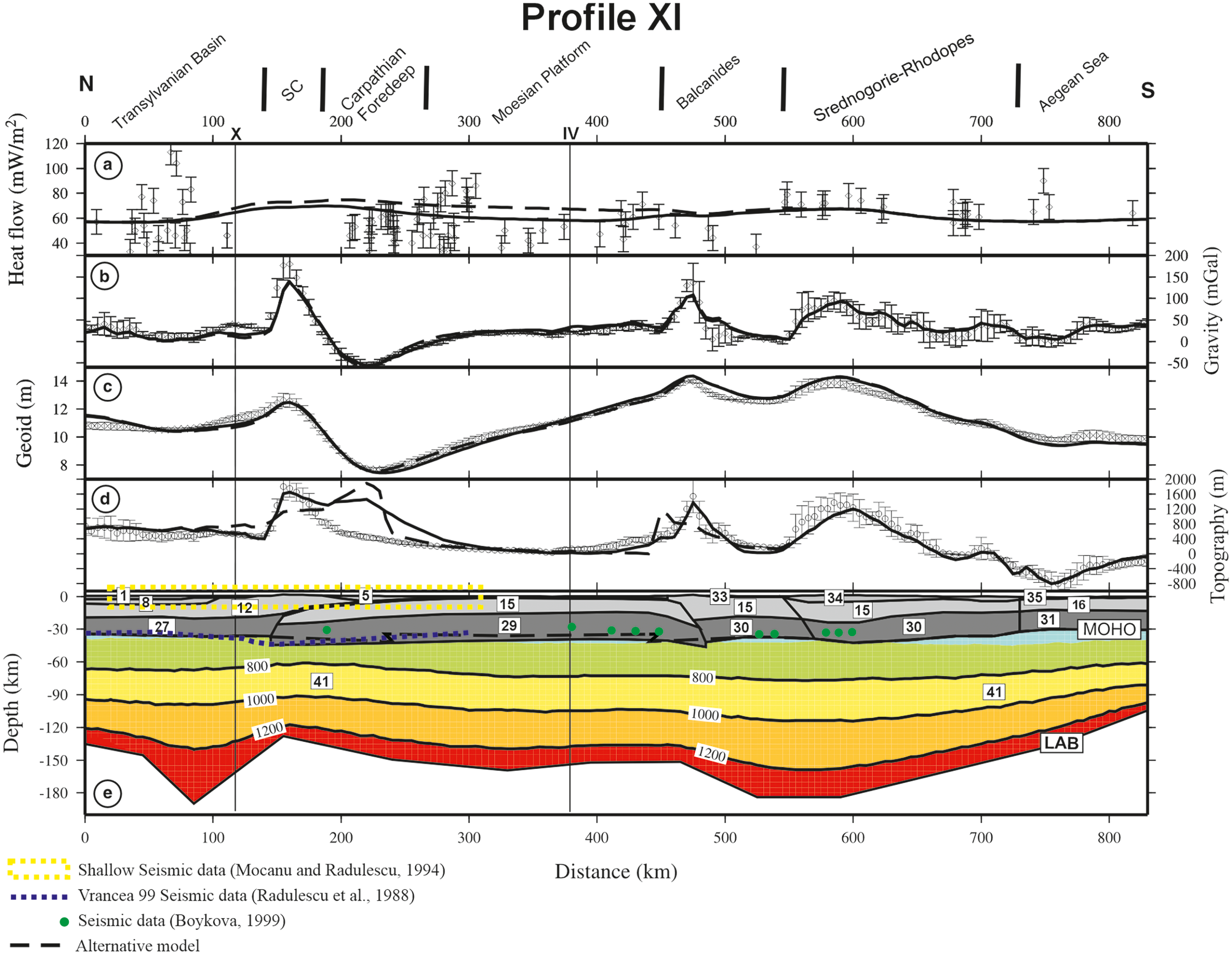
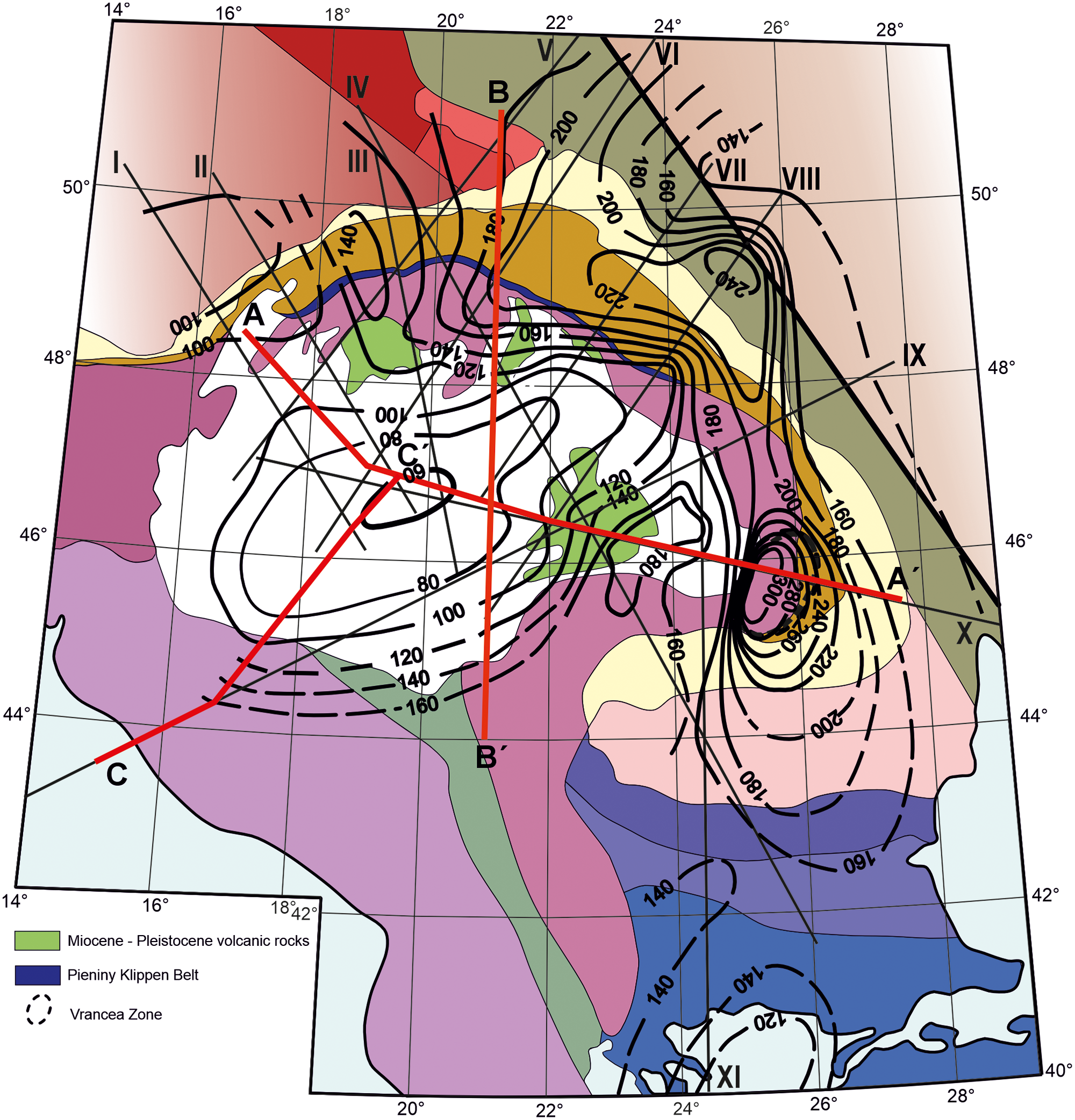
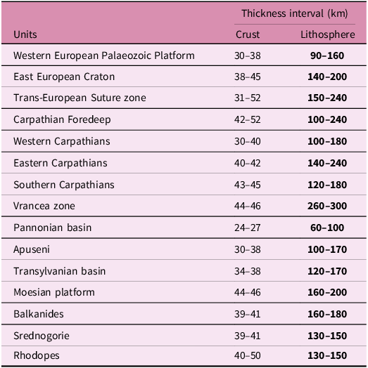
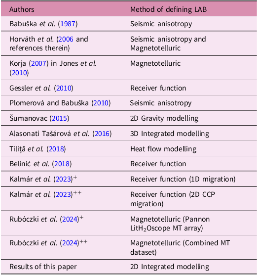
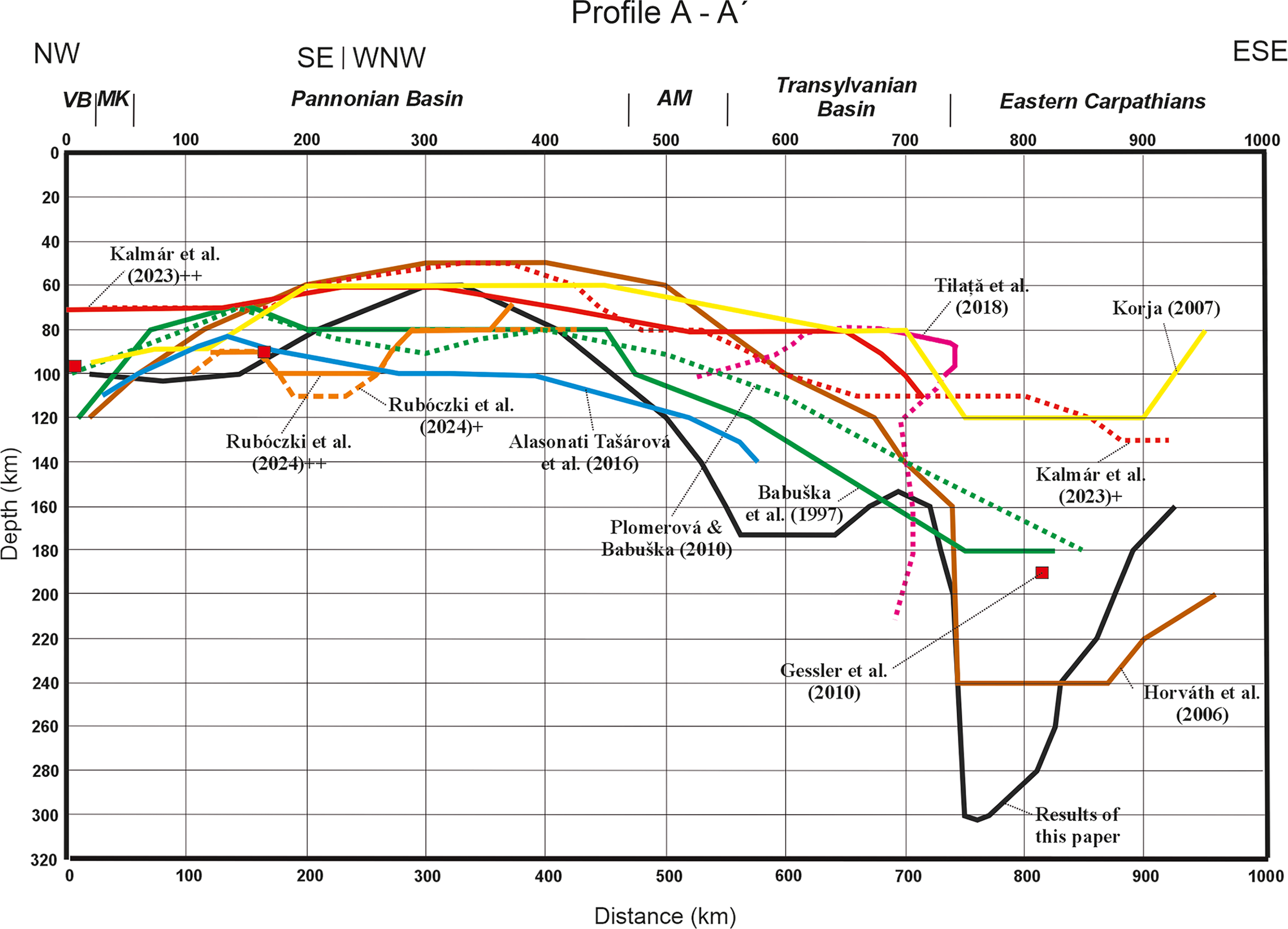
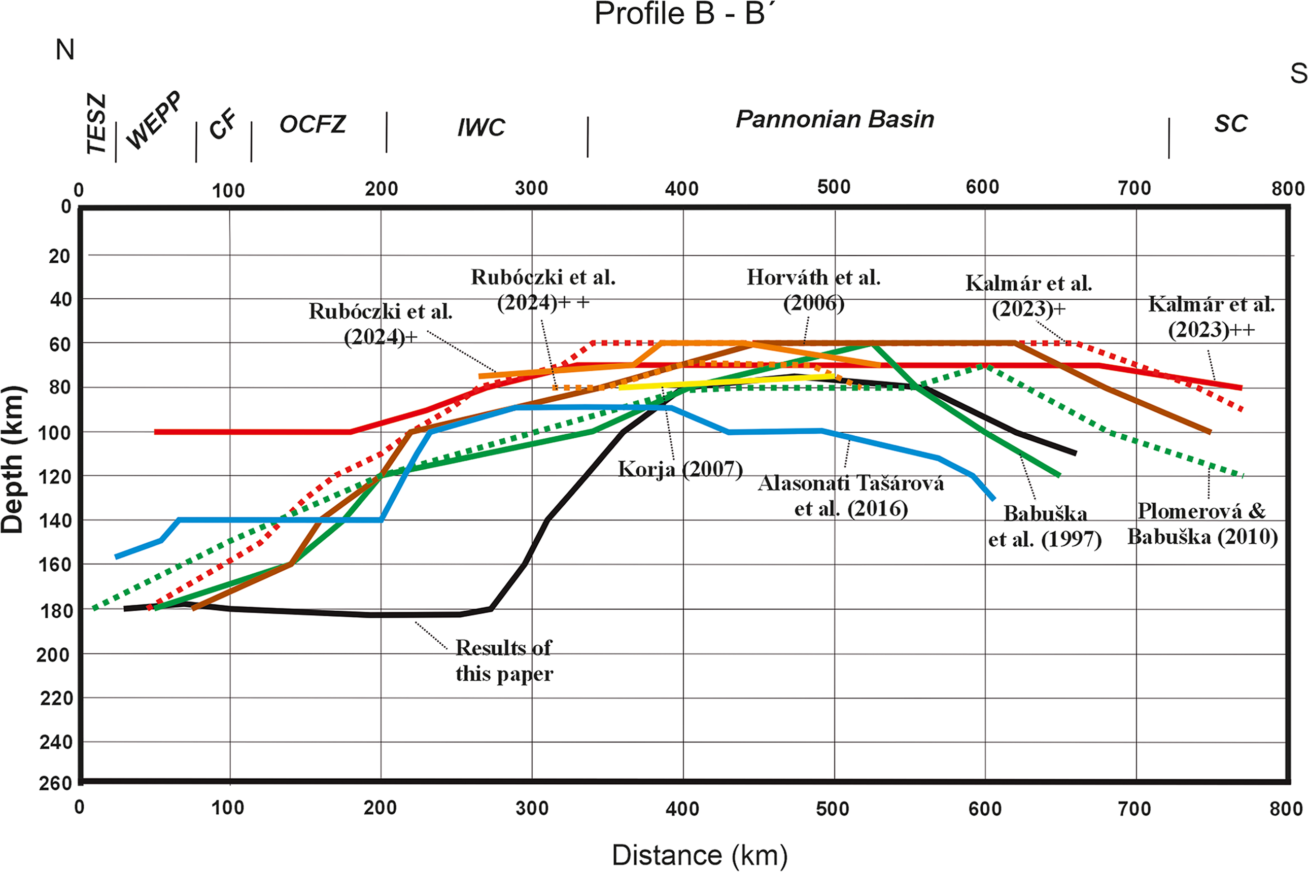
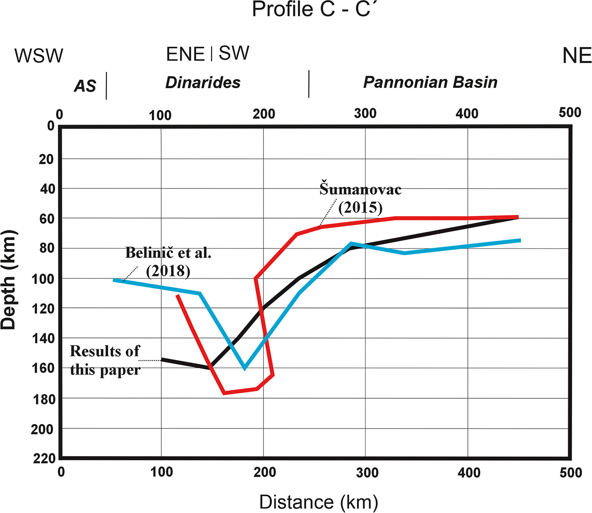

 Open access

