1. INTRODUCTION
Data are often available at different levels or at different frequencies. In cross sections, relevant data may be available at a macro level (industries) and at a micro level (firms), where the different levels give rise to different models, estimates, and forecasts. The models are often estimated by separate offices and statisticians, although they are clearly related to each other. For example, Marcellino, Stock, and Watson (2003) forecast aggregate Euro-wide inflation (macro) and country-specific inflation indexes (micro), and Hendry and Hubrich (2005) study aggregate forecasts of Euro-area inflation (macro) and five subcomponents: unprocessed food, processed food, industrial goods, energy, and services prices (micro). In the empirical part of this paper we shall consider an application in the time domain: quarterly (“macro”) and monthly (“micro”) forecasts for the Euro yield curve.
If all data were available to us at both levels, combining data would lead to efficiency gains. We shall assume, however, that we have no access to the underlying data but that we do have information on the one-period-ahead forecasts, both at the micro level and at the macro level. We now wish to combine these forecasts to obtain better forecasts at both levels, taking into account our knowledge of the relationship between the two levels.
In a linear world, the models at the two levels would be analogous,1
The study of perfect aggregation can be traced back to Theil (1954). This aggregation is very restrictive, and “perfect aggregation” tests usually favor the disaggregated model; see Pesaran, Pierse, and Kumar (1989).
There are several reasons why the macro model may not be just a (weighted) average (or sum) of the micro models. First, the macro observations are usually measured more precisely than the micro observations. Second, the transition from one level to another can be nonlinear. For example, some shocks are dampened in the long run.
There is an extensive literature on combining models or forecasts at the same level. Bates and Granger (1969) show that optimal forecast combination reduces the variance. More recently, Leung and Barron (2006) use risk terminology and provide evidence that the performance of a mixture is superior to the best of the individual models. Hendry and Clements (2004) provide an extensive survey of the literature and list the advantages one can expect from pooling forecasts. Yang (2004) gives theoretical results for combining procedures and derives risk bounds to quantify the potential gain and the “price” of linearly combining forecasts. Other useful surveys are provided by Clemen (1989) and Diebold and Lopez (1996). Bayesian model averaging (Lancaster, 2004, p. 101) has gained popularity because of its natural interpretation and good performance in practice; see also Raftery, Madigan, and Hoeting (1997) and Hoeting, Madigan, Raftery, and Volinsky (1999).
The literature on the combination of models and forecasts at different levels is much less extensive. Imbens and Lancaster (1994) offer an excellent solution, assuming availability of all micro data and macro information in the form of moment restrictions. Employing the generalized method of moments (GMM) methodology, they thus obtain more precise estimates at the micro level. Their analysis is constrained to one time period only and to the availability of all micro data. Magnus, van Tongeren, and de Vos (2000) offer a solution from a Bayesian perspective in the context of national accounts estimation. More recently, Hendry and Hubrich (2005) use a simple intuitive vector autoregression (VAR) example and demonstrate the predictability of the aggregated error from a disaggregated information set, thus motivating the combination of data sets.
The contribution of this paper is not on model averaging but is on the combination of information at different levels of aggregation. Going from the detailed (micro) level to the more general (macro) level can usually be achieved through summation or averaging. Our main objective, therefore, concerns the opposite direction, that is, using macro data to improve micro forecasts. This is the first way in which this paper differs from most of the literature on combining models and forecasts: we consider models at different levels. The second is that we do not assume that all data are available to us. We propose a two-level hierarchical model, which allows us to update the micro forecast on the basis of the macro forecast. The proposed method has a natural interpretation and shows good performance in Monte Carlo simulations.
The paper is organized as follows. In Sections 2 and 3 we provide the theoretical framework and derive the proposed forecasts. In Section 4 we present Monte Carlo evidence in a simple setup (the base scenario), and in Section 5 we consider more realistic situations, involving measurement error and other deviations from the base scenario. Section 6 extends the procedure to time series. An empirical application in Section 7 shows the benefits of combining monthly and quarterly forecasts for the Euro yield curve. Our conclusion in Section 8 is that a simple and robust forecast combination rule performs uniformly well and has, in addition, a minimum mean squared error, a least squares, and also a Bayesian interpretation. Appendix A discusses a somewhat counterintuitive result about linear combinations, whereas Appendix B summarizes the data used in the empirical example.
2. A TWO-LEVEL HIERARCHICAL MODEL
We assume that information is available at two levels: the macro level and the micro level. The macro level provides aggregate information, whereas the micro level provides disaggregate information, thus giving more detail for the components of the macro level. The macro level is indexed by t = 1,…,T; the micro level, in addition, by j = 1,…,p.
For the two levels we may have different models and different data sources. At the macro level we assume that data are available on the variable of interest ηt together with [ell ] × 1 vectors of exogenous explanatory variables zt. For simplicity, we assume a linear model

where {ut} is unobservable independent and identically distributed (i.i.d.) random noise with mean zero and variance σu2 and zt−1 is revealed at the end of period t − 1. If

denotes the ordinary least squares (OLS) estimator of γ based on T observations, then the macro forecast is given by

.
The data at the more detailed micro level consist of the vector of variables of interest yt := (yt,1,…,yt,p)′ together with p × k matrices of exogenous explanatory variables Xt. We assume again a linear model

where the vectors {vt} are unobservable i.i.d. random noise with mean zero and variance matrix Σv and Xt−1 is revealed at the end of period t − 1. If

denotes the generalized least squares (GLS) estimator of β based on T observations, then the micro forecast is given by

.
The data for the macro model are compiled in a macro office, and γ is estimated by a macro statistician. The data for the micro model are compiled in a micro office, and β is estimated by a micro statistician. The two offices and the two statisticians may or may not talk to each other. Thus, some of the information used by one statistician may also be used by the other but not necessarily so. The two levels are related to each other, even though the macro and micro statisticians do not utilize this relationship. In the background lives the linear constraint

where a is a known p × 1 vector. For example, if a = ıp, the vector of ones, then the macro observations are the sum of the micro observations, and if a = ıp/p, then the macro observations are the average of the micro observations. As a result, the two levels may be (and probably will be) correlated, but we shall assume that this correlation exists only within the same time period. Hence, cov(ut,vt) may be nonzero but cov(us,vt) = 0 for s ≠ t. We emphasize that we do not require the linear constraint ηt = a′yt to hold for every t. This would be the case of perfect model aggregation, which is rare in practice. If one, nevertheless, encounters this case, then the micro model contains the best information for both (micro and macro) levels.
The macro statistician provides a macro forecast

with an estimated variance

, and the micro statistician provides a micro forecast

with an estimated variance matrix

. (We will see later that only the relative precisions matter.) Our task is to combine the two forecasts, making use of all available information. In particular, we wish to obtain optimal one-period-ahead forecasts

(micro) and

(macro), satisfying the micro-macro relationship

Note that we do not assume that ηt = a′yt holds at t = T + 1; only that the forecast satisfies (3). Note also that our assumption on the availability of data rules out the possibility of estimating of (1) and (2) jointly. We emphasize that the linearity assumptions in (1)–(3) are made for simplicity only and do not essentially affect our analysis.
We have two forecasts of ηT+1, one based only on macro data and one based only on micro data:

We wish to improve the forecasts at both levels, and we propose the combined macro forecast as the linear combination

in the spirit of Bates and Granger (1969). Conditional on the choice of α, this provides a common-sense improvement of the macro forecast. We call (4) a linear combination rather than a weighted average, because α may not lie between zero and one if the correlation between

and

is high and positive. This is somewhat counterintuitive, and Appendix A therefore provides a justification and explanation.
Two questions now arise. First, how do we choose α? Second, how do we update the micro forecast, given the improvement of the macro forecast? We shall discuss the second question first.
2.1. Updating the Micro Forecast
We assume first that α is known and that the macro forecast is given by (4). Given the improvement at the macro level, we now update the micro forecast.
Letting

, this is achieved by choosing y to maximize

subject to

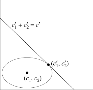
Under normality, the solution is the point with the highest probability in the micro model satisfying the macro restriction. In the two-dimensional case, Figure 1 illustrates the intuition. We have a point estimate (c1,c2) and the associated probability distribution, and we want the sum of the two estimates to be equal to c′. To include this additional information, we choose the ellipse (constant-probability contour) that is tangent to the line c1′ + c2′ = c′. The tangent point satisfies the restriction and is the most probable point given the probability distribution. In the special case where the forecasts c1 and c2 are not correlated, they will be adjusted proportionally to their variances. In the special case where the variance of c1 is zero, all adjustment will be absorbed by c2.

Update procedure in the two-dimensional case.
The normality assumption is of course a simplification. We use it here because of its central role as an approximating distribution and because it provides explicit and intuitively clear results. Our procedure can be generalized to other densities, but a closed-form solution will then typically not be available and numerical optimization has to be performed.
The solution to (5) is given by

which can be calculated if we replace Σ by

and if we know α. Note that the forecast (6) is biased, because the expectations of

and

are, in general, not equal. Thus we obtain a macro forecast

and a micro forecast

, satisfying the restriction

and taking into account information at both levels.
2.2. The Choice of α
We next address the question how to choose α. We shall employ the mean squared error criterion as our guiding principle, although this criterion has some drawbacks (Clements and Hendry, 1993) and some other criteria have recently been proposed by Diebold and Kilian (2001), Inoue and Kilian (2006), and Yang (2004).
The mean squared error of the forecast (6) is given by

where

and


Hence,

—considered as a function of α—is “small” if and only if (αq − c)(αq − c)′ is “small.” The latter matrix has rank one, and it possesses one positive eigenvalue (αq − c)′(αq − c), which is minimized for

Choosing α = α1 thus minimizes the trace of

.
3Instead of the trace we might also consider minimizing

. This leads to α1* = a′c/a′q. One may verify that α1 = α1* if and only if (a′Σa)(a′Σπ) = (a′Σ2a)(a′π), which is the case, for example, when π = 0 or Σ = I or Σa = π.

we obtain

and hence

where

and

Because information on micro and macro forecasts reaches us separately, we do not have a direct estimate of π. We can, however, estimate π from a history of forecasts

, if such a history is available. Quite often, such a history will not be available. Interestingly, our simulations (to be discussed later) indicate that the assumption π = 0 is a reasonable, often optimal, assumption to make.
If the two processes {ut} and {vt} are uncorrelated, we have π = 0, and hence

which is a number between zero and one. For small values of the components of π, α1 also lies between zero and one. But if the correlation between

and

is positive and high, then α1 does not necessarily lie between zero and one.
To compare the various combined forecasts we consider the trace of

, which we denote generically by τ2. For α = α1 we obtain from (7)

and for α = α2

3. A DIFFERENT ROUTE
The method of the previous section can be summarized as follows. Given a macro forecast

and a micro forecast

, we minimize the quadratic form

subject to the restriction

This produces a forecast

. We then choose α such that the mean squared error of

is minimized.
We now describe a second possible method, based on the idea that we should choose y such that a′y is close to

and that y is close to

. Thus we minimize

where

We can also phrase this problem as the regression problem
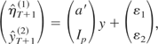
with

This formulation implies that

, so that E(δ) = 0. After somewhat tedious but straightforward calculations we find the GLS solution as

with

Note that we introduce α3 to connect the GLS solution (12) to the previous solutions. There is, however, no optimization over α in this case. In this sense one can think about the GLS solution as optimal for both micro and macro level.
The forecast (12) is unbiased, and its variance is given by

so that

which should be viewed as the analogue to τ12 in the previous section. There is no theoretical inequality between τ12 and τ32. For example, in the special case when there is no inconsistency between the models (so that zT′γ − a′XTβ = 0), and the variance structure is simply Σ = Ip and a = ıp, we find

The difference between τ12 and τ32 then depends on the relationship between

and both τ12 < τ32 and τ12 > τ32 are possible.
Given the micro forecast, the macro forecast is then given by

In the special case where π = 0 we obtain

with

The variance of this forecast is

so that

Notice that τ42 ≤ τ22 as a result of the fact that in the derivation of τ42 we have assumed that the inconsistency parameter satisfies E(δ) = 0.
The result (15) can also be phrased in Bayesian terms by considering macro data together with a micro prior:

Using Theorem 1 of Magnus, van Tongeren, and de Vos (2000), we then obtain the mean and the variance of the posterior distribution of

as (15) and (17), respectively.
Finally, if more information were available than there is, we could try to incorporate macro information in the micro model, motivated by Hendry and Hubrich (2005). For example, we might assume

where the vector h will typically be the unit vector ı and a′h > 0. The formulation (19) implies that a′yt is a weighted average of a′Xt−1β and zt−1′γ, apart from some noise a′ζt.
We emphasize that this model requires knowledge of the separate micro and macro data sets, which we do not have. Nevertheless it is of interest to compare our feasible forecasts with some forecasts that require more data, because this provides information on the sensitivity of the feasible forecasts.
Let

and

denote the OLS estimators in this model. The unrestricted estimators

and

are related to the restricted estimator

(under the restriction γ = 0) by

for some matrix Π1. Hence the micro forecast is given by

where Π′ = (Π1′ : I) and its mean squared error is

where

We see that

in this case can be larger or smaller than

.
4. MONTE CARLO EVIDENCE: THE BASE SCENARIO
To compare the proposed forecasts and to assess the possible improvement resulting from the use of macro information, extensive simulations were performed on which we now report. First we generate five regressors:


These regressors can be combined in various data sets. We consider five data sets with two regressors and five with three regressors, as follows:

The number of regressors is therefore k = 2 or k = 3. Given one of these 10 data sets, we generate the p × k matrices Xt−1 for t = 1,…,T. We consider T = 24 or T = 96 years and within each year p = 3 or p = 9 micro units.
4.1. The Data-Generation Process
For the base scenario, the micro data are generated by

where all k elements of β are equal to one. Letting σv2 = 1 we take independent draws from the N(0,σv2) distribution, generate the p × 1 vectors vt, and compute yt. The macro data are exact aggregates of the micro data, so that

where the aggregation vector a = ıp/p. The macro data are thus generated by

where all k elements of γ are also set equal to one, ut = a′vt almost surely, and σu2 = σv2a′a = 1/p.
4.2. The Model
The base model is the same as the data-generation process, except that the micro and macro statisticians do not know the exact relationship between the two models and hence do not utilize the relationship ut = a′vt (almost surely).
The OLS estimator in the micro model (21) is given by

and the one-period-ahead forecast can be computed as

. All sums, unless otherwise indicated, are for t = 1,…,T. The variance of

is

The macro model is given by (22). The OLS estimator for γ is

and the one-period-ahead forecast can be computed as

. The residuals are defined as

and the variance estimates as


One may verify that

because cov(yt,ηt) = cov(vt,a′vt) = σv2a. Because the micro and macro models are estimated separately, the fact that ut and vt are correlated is not known and not used by our macro and micro statisticians. As a result, cov(yt,ηt) is not estimated by

but rather by

, which is not the same. The estimate for π is then given by

and, although π = Σa, it is not true that

. We note that, in practice, we cannot compute this estimate, because our information consists only of the two forecasts and their precisions. In the simulations we can, however, compute the estimate, and it allows us to study the sensitivity of the feasible forecasts. All Monte Carlo experiments were performed with 10,000 replications.
4.3. Forecast Comparisons
We now compare the various forecasts assuming the data-generation process and the models from the base scenario. As a target for comparison, we shall use the forecast (6),

considered as a function of α. The trace of its mean squared error is

also a function of α. We define τ02 as the minimum value of τ2(α), and we call τ0 the target root mean squared error (RMSE). We emphasize again that, given the data constraints on our statistician, only three of the six forecasts can actually be computed in practice, namely, the micro forecast and the forecasts whose RMSEs are labeled τ2 and τ4. The remaining three forecasts are presented for comparison and sensitivity purposes only.
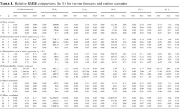
Table 1a gives the results for the micro forecast and for the five competing forecasts. In each case we present

that is, the performance of the relevant RMSE relative to the target RMSE. Because π = Σa in the base model, we obtain

in both (6) and (12). Hence, the forecast based on micro data only (and ignoring macro information) is the optimal forecast in this case. The relative loss compared to itself (Table 1a(1)) is obviously zero.
Relative RMSE comparisons (in %) for various forecasts and various scenarios

We do not present the results for each data set; instead we provide only the minimum, maximum, and median of the relative RMSE among the different data sets. If we replace the optimal α (i.e., α1) by its estimate

, we obtain τ1; see Table 1a(2). For most data sets, the results are close to Table 1a(1) because

is close to α1. But for some data sets the relative loss is very large. Setting π = 0 we obtain

and τ2, and the relative loss is reported in Table 1a(3). This should not be as good as Tables 1a(1) and 1a(2) because in fact π ≠ 0, but in fact the performance is better, both in terms of “worst-case scenario” (max) and in terms of the median.
In Tables 1a(4) and 1a(5) we report the RMSE for the forecasts (12) and (15). The forecast (12) does not perform well for some data sets, whereas the forecast (15) does perform well. Table 1a(4) is very close to Table 1a(2), whereas Table 1a(5) is slightly worse than Table 1a(3) because α2 < α4 because of the bias term.
Finally, the model that incorporates macro information into the micro model leads to forecast (20). Here we estimate parameters that are in fact zero, and hence we lose efficiency. This is reflected in Table 1a(6).
5. DEVIATIONS FROM THE BASE SCENARIO
In real-life applications, the micro model and the macro model will deviate more than in the idealized situation of the previous section. We now investigate four scenarios that mimic situations as they might occur in practice.
5.1. Measurement Errors in the Micro Regressors
We assume that there are two regressors (k = 2, data sets 1–5) and that the data are generated as in the base case. However, the second regressor is badly measured at the micro level, so that we observe xt−1,2* = xt−1,2 + ζt−1 instead of xt−1,2. The {ζt} are i.i.d. N(0,σζ2), and they are independent of all other errors. The estimates and forecast at the micro level are thus based on Xt−1* := (xt−1,1,xt−1,2*). The effect of the measurement error will be that the OLS estimator

is inconsistent with a bias toward zero.
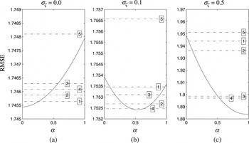
Measurement errors can either accumulate or dampen when aggregated. Here we assume that they dampen and in fact that measurement errors are absent in the macro model. Thus, the regressors in the macro model are zt−1 = Xt−1a and not zt−1 = Xt−1*a. In Figure 2 we plot τ(α) (solid line) for three values of σζ, namely, 0.0, 0.1, and 0.5. The case σζ = 0 is identical to the base scenario discussed in the previous section. Hence, the minimum τ0 occurs at α = 0. The values of τ1,…,τ5 are also plotted, and we see (for this specific data set) that τ1 performs best and τ5 worst, in correspondence to Table 1.

Effect of measurement errors in micro regressors, T = 24, p = 3, data set = 3, for three values of σζ.
If σζ > 0, then the minimum of τ(α) will not be at α = 0. In this specific example, τ4 performs best. This is the simple “Bayesian” solution, ignoring information on π.
Tables 1b and 1c provide more detailed information. When σζ = 0.1 (Table 1b), the optimum is not at zero, and the naive micro forecast is not optimal any more. This is reflected in Table 1b(1). Table 1b(2) (reporting on τ1) is further away from the optimum, because of the misspecification, which implies that α1 is no longer the optimum value for α. Table 1b(3) is close to the optimum, showing that the wrong assumption π = 0 is less damaging than the misspecification. Table 1b(4) is again similar to Table 1b(2), but, because the optimal α is not zero, there is no strict dominance in this case. Table 1b(5) (reporting on τ4) is uniformly closer to the minimum than Table 1b(4), which shows again that information on π is not necessarily useful. The explanation for Table 1b(6) is similar to Table 1a(6) with the addition that we not only estimate zeros in this case but also have a measurement error bias.
In Table 1c we consider the case where σζ = 0.5. The differences between the various forecasts are larger now than in the case when σζ = 0.1. The naive micro forecast in Table 1c(1) is not a good forecast any more. The correct specification assumption remains more important than the assumption that π = 0, so that Tables 1c(2) and 1c(4) are dominated by (bigger than) Tables 1c(3) and 1c(5), respectively. The forecast corresponding to τ4 is the clear winner in this case.4
Notice the negative number in Table 1c(5), implying that τ4 < τ0 in one of the data sets (number 4). This can happen, because the α-curve and therefore the theoretical optimum is calculated by averaging the simulation results, keeping α fixed. When α is estimated, then the average is not necessarily on the α-curve (this is the reason why on the pictures, when α is estimated, the results are shown as a straight line rather than a point). Therefore it is possible that τ1,…,τ4 are less than the simulated optimum. This is, however, a rare event.
5.2. Nonavailability of Some Micro Regressors
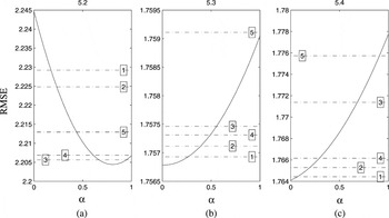
We now assume that there are three regressors (k = 3, data sets 6–10). However, the third regressor is only available at the macro level, not at the micro level. As a result we have Xt−1* := (xt−1,1,xt−1,2), whereas Xt−1 := (xt−1,1,xt−1,2,xt−1,3). When one of the regressors is not available at the micro level, then the forecast performance depends on which regressor is not available and how much useful information is lost. Figure 3a illustrates that the minimum of the τ(α)-curve is not at α = 0 and gives the RMSEs for the five competing forecasts for one data set. Table 1d provides more detailed information and shows that the loss can be substantial. For example, in Table 1d(1) the naive micro forecast suffers badly from the omitted variable bias, in particular in one of the data sets (number 7). (These outliers are the main reason for using the median rather than the mean in reporting the simulation results.) Tables 1d(2) and 1d(3) are slightly closer to the target, but not as much as Tables 1d(4) and 1d(5), which shows that the bias term in α1 is poorly estimated. In most cases, Table 1d(4) gives better result than Table 1d(5).

Effect of three types of misspecification, T = 24, p = 3, data set = 8.
The model that incorporates macro information into the micro model (forecast (20)) is interesting in this case. In the previous scenarios, this forecast was far from the optimum, but here it gives a better result than the minimum of the α-curve. This is not a surprise, because we are using a macro regressor as a proxy for the corresponding micro regressor (which is not available) and this proxy is a very good proxy.
5.3. Nonimportance of Some Macro Regressors
Next we assume that there are three regressors (k = 3, data sets 6–10) and that the third regressor satisfies a′xt−1,3 = 0 for all t. The statistician does not know this, and so the micro model is estimated without imposing the restriction. In the macro model, all observations on zt−1,3 will be zero, and so this regressor is dropped from the model and the macro estimates and forecasts are based on two regressors only.
We see from Figure 3b that the minimum of the τ(α)-curve is at α = 0. Hence it is no surprise that the forecasts labeled 1 and 2 perform well in this case. We might expect efficiency gains because we estimate only two (rather than three) parameters at the macro level, but the efficiency gain is very small and Figure 3b looks very similar to Figure 2a. Table 1e confirms that the results are similar to the base scenario.
5.4. Correlation at the Micro Level
Finally, it may happen (indeed, it is likely) that the micro units are correlated, so that vt ∼ N(0,Σv), where Σv is not proportional to the identity matrix. Here we assume that

where J := ıpıp′/p is an idempotent matrix of rank one and the coefficients are θ1 := 1 + (p − 1)ρ and θ2 := 1 − ρ. The statistician, however, is unaware of the correlation. We take ρ = 0.5. The data-generation process has changed, but the models are still the same.
In this case the theoretical minimum is often obtained for α < 0; see Figure 3c. We know that this is theoretically possible, and truncation at zero would lead to poorer performance. The forecasts reported as τ1 and τ3 perform poorly; the other forecasts perform reasonably well.
6. EXTENSION TO TIME SERIES
Let us summarize our findings so far. Our purpose was to construct an improved micro forecast

in the situation where we are given a macro forecast

with estimated variance

and a micro forecast

with estimated variance matrix

and where, in addition, we wish the improved forecasts to satisfy a constraint

. Based on the preceding theory and simulations we propose the micro forecast

where

and

denotes the weight in the associated macro forecast

The proposed micro forecast has a minimum mean squared error interpretation and is also optimal in a least squares and a Bayesian framework.
In a time-series framework the aggregate level (e.g., a quarterly model) forecasts the average outcome for several periods (say, the average over three months in one quarter), whereas the more detailed level (a monthly model) forecasts each period (month) separately. In this sense one can think about the aggregated (quarterly) level as a “macro” model and about the detailed (monthly) level as a “micro” model. This provides the link between the current section and the previous sections.
Implicit in the theory developed so far is that the data become available once per period, so that the additional data required to forecast period T + 1 all become available at the same time, namely, at the end of period T. This is reasonable if we consider p micro units in one macro unit, such as p firms in one industry or p industries in one sector or p sectors in one economy. But it is not reasonable in a time-series framework where we consider p = 3 months in one quarter or p = 4 quarters in one year. In that case the relevant micro data will become available during the year and not just at the end of the year. An extension of the theory is thus required.
The extension is straightforward. Suppose that p1 micro periods have passed so that p − p1 micro periods are to be forecasted. The first p1 elements of yT+1 are then known so that

The estimated variance matrix of this vector has the form

where Σ2 is a (p − p1) × (p − p1) matrix. At the macro level there is no new information, and so there is no need to redefine the original macro forecast

.
With these modifications of

and

we can compute the micro forecast

and the macro forecast

from (23) and (24), and the same optimality results will hold.
As we proceed through period T + 1, the original macro forecast

does not change, but the vector of micro forecasts

is updated together with its variance

. This will affect α. One would expect that the weight of the micro information increases when more information becomes available, so that α decreases. To demonstrate this intuition assume that Σ = diag(σ12,…,σp2) is diagonal and known and that a = ıp/p where ıp denotes the p × 1 vector of ones. Then α as a function of p1 will be

which obviously gives α(p1) > α(p1 + 1).
7. IMPROVING THE EURO YIELD FORECAST BY COMBINING MONTHLY AND QUARTERLY MODELS
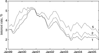
We demonstrate our theory by presenting new predictions of European interest rates, in particular zero rates; see Figure 4. As predictors we take various macro and financial series. A detailed description of the data set is provided in Appendix B.

Euro zero rates for maturities 1, 2, and 5 years.
An important feature of the European series is its relative shortness. The series starts with the introduction of the Euro in January 1999, which gives us seven full years of observations. In addition, some of the macro series are released with a half-year delay, so that the final data set consists of 78 monthly observations and 26 quarterly observations. This is an extremely short series when compared to the U.S. series, which is available from the early 1960s. There is some evidence of convergence of the yield curves of the Euro-zone countries (see, e.g., Batten and Fetherston, 2004), but this does not allow us to extend the European series significantly.
It is therefore important to use as much information as possible to get a good forecast. The annual observations cannot provide a reliable forecast, but there are enough quarterly observations to construct a reasonable model, especially because they are much less noisy than the monthly data.
The shortness of the series also explains why relatively few papers exist on the European market. In contrast, the U.S. market has been studied extensively; see Barrett, Gosnell, and Heuson (2004), Piazzesi and Swanson (2004), and Diebold, Rudebusch, and Aruoba (2006). An excellent survey and empirical comparisons can be found in Diebold and Li (2006).
We shall be concerned with the prediction of maturities of 1, 2, and 5 years, rather than with the term structure of interest rates. The main reason is that bonds with higher maturities are not exercised during the observed period, so that there is no evidence of how well they were priced. We predict the selected yields directly rather than using factor models, because each additional step (extracting factors in this case) consumes information and the information is very limited in our case because of the short history. Model selection and pretesting issues are ignored. The final models are similar to the models typically used for the U.S. yields. The final improvement of the forecast is uniform over different possible sets of monthly and quarterly models.
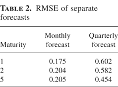
To compare different forecasts we look again at the RMSE. The first half of the sample is used for estimation, and we use the second half for out-of-sample forecasting. The forecasts are based on the linear models (1) and (2) with the regressors described in Appendix B. For both models we use a one-step-ahead linear forecast with an increasing window. The results for the separate monthly and quarterly forecasts are given in Table 2. One should not conclude from Table 2 that the monthly model is better than the quarterly model, because they are not nested. Moreover, they are structurally different and use a different number of observations and predictors. However, one can see that the monthly model forecasts short-term yields better than long-term yields, whereas the quarterly model is more accurate for the long-term yields. Notice that in this case micro and macro data are both available but that the micro data do not become available at once—they come in three installments.
RMSE of separate forecasts

The quarterly yield is just the average of the monthly yields, but for the forecasts this is not necessarily the case. The procedure from Section 6 allows us to bring the quarterly and monthly forecasts in accordance with each other by taking the restriction vector to be

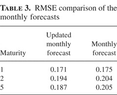
. Combining monthly and quarterly forecasts we obtain the results presented in Table 3.
RMSE comparison of the monthly forecasts

The updating procedure improves the monthly forecast. One can argue that the improvement is not significant, but if it is translated into basis points (bp: 100 bp = 1%), which is a standard measure for the bond market, then the improvement is 40, 100, and 180 bp, respectively, for 1, 2, and 5 years to maturity, which is considerable.
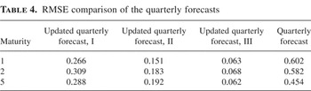
This is for the monthly (“micro”) forecasts. For the quarterly (“macro”) forecasts we have three updated versions; see Table 4. The first update (I) is made at the beginning of the quarter, when the monthly forecasts are made with one-, two-, and three-step-ahead models. At the beginning of the second month, the first month has been observed, and one- and two-step-ahead forecasts are used for the second and third months. This gives the second update (II). Finally, the third update (III) is made at the beginning of the third month when the values for the first and second months are known; the third month is forecasted with a one-step-ahead model. As Table 4 reveals, with the new monthly information received we can improve the quarterly forecast considerably, and the more information revealed, the more accurate our forecast becomes. This simple illustration thus demonstrates the importance of combining information at different levels and also suggests that our proposed method works well in practice.
RMSE comparison of the quarterly forecasts

8. SUMMARY AND CONCLUSIONS
The purpose of this paper was to construct an improved micro forecast

in the situation where we are given a macro forecast

with estimated variance

and a micro forecast

with estimated variance matrix

and where, in addition, we wish the improved forecasts to satisfy a constraint

. Based on the theory and simulations in this paper we propose the micro forecast (23) and the macro forecast (24). We emphasize again that only the relative precisions of the forecasts are required.
The proposed forecasts are simple and robust. The robustness is investigated in the simulations in two ways. First, by assuming (τ1 and τ3) that we can estimate the correlation π, which in most cases we can not. The additional information does not appear to help us; in fact, the contrary is the case. Second, by assuming that all data are available and that we incorporate the macro regressors in the micro model (τ5); this too does not appear to be a fruitful extension.
The proposed forecast performs uniformly well, both on average (considering the median relative loss of the various data sets) and from the worst-case scenario (maximum relative loss) viewpoint. Various types of misspecification were considered: micro measurement error, absence of one of the micro regressors, a macro restriction, and micro correlation. In all these cases our proposed forecast performs well.
An empirical example concerning forecasts of the Euro yield curve confirms that a time-series modification of our procedure improves both monthly and quarterly forecasts.
The method can be generalized to more than two levels, to nonlinear models such as factor models (Stock and Watson, 2002a, 2002b), to nonlinear restrictions, and to nonnormal densities.
APPENDIX A: Estimation of the Common Mean of a Bivariate Distribution with Known Variance
Suppose we have two measurements on an unknown quantity θ:

where (ε1,ε2) follows a bivariate normal distribution with mean zero and known variance

If ε1 and ε2 are uncorrelated (σ12 = 0) and the two variances are equal, then we estimate θ by

. If ε1 and ε2 are uncorrelated and the two variances are not equal, then we estimate θ by

which is a weighted average of y1 and y2, where the weight α lies between zero and one.
Now consider the case where ε1 and ε2 are correlated. Then we also obtain

but now with

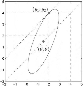
We see that α does not necessarily lie between zero and one. In particular, α < 0 if and only if σ12 > σ22, and α > 1 if and only if σ12 > σ12. Figure A.1 illustrates this situation. It presents one constant-probability contour for the case σ1 = 1, σ2 = 2, and σ12 = 1.5. Hence the correlation is r = ¾. Our two observations take the values y1 = 2 and y2 = 4, so that we obtain α = 1.25 and

, which clearly lies outside the interval (y1,y2).

Constant-probability contour for the case cov(y1, y2) > var(y1).
At first glance this may seem unsatisfactory. We have two observations 2 and 4 and an estimate of 1.5. At second glance, however, it becomes clear that this is the correct solution and that we should not force the solution to be between the two observations.
Consider the extreme situation where r = 1 and σ1 ≠ σ2. Then we have y1 = θ + σ1ε and y2 = θ + σ2ε, where the common noise ε satisfies ε ∼ N(0,1). In this case,

must lie outside the interval (y1,y2). We simply solve the two equations in two unknowns (θ and ε) and find

with

The “weight” α in this case is either larger than one (if σ1 < σ2) or smaller than zero (if σ1 > σ2).
Consider another situation where

where ε has mean zero and is distributed independently of y1. In this case cov(y1,y2) = σ12 and

. The observation y1 is a sufficient statistic for θ, and the information contained in y2 is superfluous.
We conclude that—in the presence of correlation—“weights” may lie outside the (0,1) interval.
APPENDIX B: The Data
The data used in the empirical example of Section 7 have been obtained from Eurostat Web site http://europa.eu.int/comm/eurostat and cover the period from January 1999 until June 2005. We analyze the 12 Euro-zone countries Belgium, Germany, Greece (from 1 January 2001), Spain, France, Ireland, Italy, Luxembourg, the Netherlands, Austria, Portugal, and Finland.
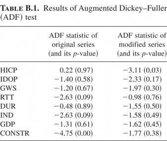
Some of the series, especially indices, contain a unit root. The formal unit root analysis is presented in Table B.1. Following Piazzesi and Swanson (2004) we use year-on-year log differences to remove the unit root. This is convenient, because the transformation is uniform for monthly and quarterly data. Moreover, the transformation removes possible traces of any seasonal component.
Results of Augmented Dickey–Fuller (ADF) test

The monthly model includes the 15 predictors described subsequently and a constant.
HICP: Inflation is captured by the consumer price indices, measured for each country separately and combined in one harmonized index. We use the harmonized index provided by Eurostat. The series contains a unit root, and so we use its year-on-year log change.
IDOP: Producer prices are measured by the index of industrial domestic output prices. The series contains a unit root, and so we use its year-on-year log change.
GWS: As an analogue of the nonfarm payrolls in the United States, we use the seasonally adjusted index of gross wages and salaries of total industry excluding construction. The series is again nonstationary, and we use its year-on-year log change.
HUNE: Unemployment is measured by the seasonally adjusted harmonized unemployment index of all age classes including males and females. Similar to the price index it is measured for each country separately and then combined into one harmonized measure using the weighted sum transformation.
RTT: The condition of industry and services is reflected by the seasonally adjusted retail trade turnover index. The series contains a unit root, and so we use its year-on-year log change.
DUR: The seasonally adjusted index of the industrial production of consumer durables is differentiated to remove the unit root.
IND: Stationary adjusted version of the industrial production index for the total industry excluding construction.
DR: The relation between the official deposit rate (DR), the official refinancing operation rate, and the official lending rate is kept fixed (with the exception of a short period January–March 1999) by the Central Bank with a gap of 1%. We arbitrarily choose the official deposit rate for our analysis.
EURIBOR, LIBOR: To account for other possibilities for investment we include money market short-term interest rates EURIBOR for Euro contracts and LIBOR for interbank loans in London. The LIBOR rate is taken because of the high influence this market has on the whole of Europe.
GBP, USD: We take account of international competition for investments by including the exchange rate for pound sterling (GBP) and the U.S. dollar (USD).
SPRD (three predictors): Piazzesi and Swanson (2004) find the yield spreads particularly useful for their analysis. We include three yield spreads: the spread between 2 and 1 year yields (SPRD2,1), between 5 and 2 years (SPRD5,2), and between 10 and 5 years (SPRD10,5).
The quarterly model resembles the yields-macro model of Diebold et al. (2006), which includes real activity, monetary policy, and inflation. It contains a constant, the average inflation, and the average deposit rate from the monthly data and the following three predictors:
GDP: The stationary transformation of the seasonally adjusted gross domestic product in current prices.
CONSTR: The stationary transformation of the seasonally adjusted construction production index.
CU: Percentage of the current level of capacity utilization (CU) from business surveys.