1 Introduction
1.1 Planetary context
The dynamics of planetary fluid layers often defies our physical knowledge. A fundamental understanding can be obtained with massive numerical simulations (e.g. Schaeffer et al. Reference Schaeffer, Jault, Nataf and Fournier2017). The success of this approach is somewhat surprising, considering the gap between the parameters of the simulations and the expected planetary values. Realistic numerical simulations will remain for a long time inaccessible to the computational power. Moreover, a long-term endeavour is to go beyond the spherical geometry in these models. Indeed, planetary fluid bodies are closer to ellipsoids than to spheres, for instance due to tidal effects (e.g. Chandrasekhar Reference Chandrasekhar1969; Nduka Reference Nduka1971). However, simulations in deformed spheres are very challenging. Numerical methods usually used in non-spherical geometries, such as finite elements (e.g. Cébron et al. Reference Cébron, Le Bars, Le Gal, Moutou, Leconte and Sauret2013), are not very efficient for this problem. Spectral numerical methods have been developed in (weakly) non-spherical containers (e.g. Reese, Lignières & Rieutord Reference Reese, Lignières and Rieutord2006; Rieutord, Espinosa Lara & Putigny Reference Rieutord, Espinosa Lara and Putigny2016), but they rely on non-orthogonal spherical-like coordinates (Bonazzola, Gourgoulhon & Marck Reference Bonazzola, Gourgoulhon and Marck1998) that strongly complicate the numerics. Furthermore, accounting for density variations (compressibility) is another computational burden. Thus, mainly incompressible flows have been simulated in deformed geometries (e.g. Cébron et al. Reference Cébron, Le Bars, Leontini, Maubert and Le Gal2010; Favier et al. Reference Favier, Grannan, Le Bars and Aurnou2015).
To gain physical insight, we can develop reduced global models in ellipsoids. Reduced models have proven useful to approach more realistic values in spherical convection (e.g. Guervilly, Cardin & Schaeffer Reference Guervilly, Cardin and Schaeffer2019). In ellipsoids, a first step would be to investigate the global modes of rotating compressible fluids. Indeed, the inertial modes (sustained by global rotation) play a fundamental role in rotating flows (e.g. Zhang & Liao (Reference Zhang and Liao2017), for incompressible flows). They can be triggered by orbital forcings (Le Bars, Cébron & Le Gal Reference Le Bars, Cébron and Le Gal2015) and coupled nonlinearly to yield flow instabilities (e.g. Kerswell Reference Kerswell1993, Reference Kerswell2002; Vantieghem, Cébron & Noir Reference Vantieghem, Cébron and Noir2015). Thus, reduced compressible models in non-spherical rotating domains are worth developing.
Developing such models was largely inhibited by the mathematical complexity of the ellipsoidal system (e.g. Cartan Reference Cartan1922). Analytical expressions for the acoustic modes do exist in non-rotating spheroids (Chang Reference Chang1971, Reference Chang1972) and ellipsoids (Willatzen & Lew Yan Voon Reference Willatzen and Lew Yan Voon2004). Similarly, analytical solutions of the incompressible inertial modes (Backus & Rieutord Reference Backus and Rieutord2017) exist in spheroids (Zhang & Liao Reference Zhang and Liao2017), but not in ellipsoids (except for a few, see Vantieghem (Reference Vantieghem2014)). Unfortunately, these analytical solutions cannot be extended to account for additional ingredients, notably (i) global rotation for the acoustic modes and (ii) compressibility for the inertial modes. In the latter case, extensions towards compressible models have been attempted. Yet, they were restricted to neutrally buoyant fluids, by considering specific isentropic (polytropic) states within the anelastic approximation (e.g. in ellipsoids Clausen & Tilgner (Reference Clausen and Tilgner2014)). A consistent mathematical treatment of the acoustic and inertial modes may appear as a prerequisite, to pave the way for future planetary-driven reduced models.
1.2 Experimental context
A complementary physical understanding can be obtained with experimental analogues. Despite they lack some ingredients compared to simulations, experiments can often probe more turbulent regimes (as measured by the Reynolds number). Motivated by planetary-driven applications, experiments have been conducted in spherical geometries (e.g. Kelley et al. Reference Kelley, Triana, Zimmerman, Tilgner and Lathrop2007; Triana et al. Reference Triana, Zimmerman, Nataf, Thorette, Lekic and Lathrop2014; Tigrine et al. Reference Tigrine, Nataf, Schaeffer, Cardin and Plunian2019). Similarly, planetary-driven ellipsoidal experiments have been built to mimic tidal deformations, for instance with water (e.g. Noir et al. Reference Noir, Brito, Aldridge and Cardin2001, Reference Noir, Cébron, Le Bars, Sauret and Aurnou2012; Grannan et al. Reference Grannan, Favier, Le Bars and Aurnou2016; Lemasquerier et al. Reference Lemasquerier, Grannan, Vidal, Cébron, Favier, Le Bars and Aurnou2017; Le Reun, Favier & Le Bars Reference Le Reun, Favier and Le Bars2019) or the gas-filled spheroidal experiment ZoRo (Su et al. Reference Su, Cébron, Nataf, Cardin, Vidal, Solazzo and Do2020). A major difficulty in the experimental approach is to reconstruct, from a sparse set of measurements, the velocity field within the fluid domain.
Conventional velocimetry methods, such as particle-imaging techniques, give often partial information on the flow components. In order to sample larger portions of the fluid domain, a large and flexible imaging apparatus is required. This is quite challenging to develop for (rapidly) rotating experiments. The fluid must be also seeded with neutrally buoyant tracer particles, acting as scatterers (of light or sound). Yet, buoyant tracers can float, sink or be quickly centrifuged (especially in rapidly rotating gas-filled experiments). Moreover, some methods work only in non-opaque fluids (for the part of the light spectrum probed by the sensor), such as particle image velocimetry and laser Doppler velocimetry, and, alternatives to optical techniques must be employed for liquid metal experiments (e.g. Kelley et al. Reference Kelley, Triana, Zimmerman, Tilgner and Lathrop2007; Tigrine et al. Reference Tigrine, Nataf, Schaeffer, Cardin and Plunian2019). Consequently, it is worth developing flexible imaging techniques for transparent or opaque fluids, with a large sampling domain and using non-invasive sensors.
Modal acoustic velocimetry (MAV) does match these requirements. This technique consists in the identification of the normal modes of oscillations of the fluid. Since the acoustic modes are highly sensitive to the flow properties, the observed distribution of acoustic resonant frequencies can feed an inverse problem, to gain a passive access to the (hidden) dynamics. This technique is routinely used in helioseismology and asteroseismology (e.g. Aerts, Christensen-Dalsgaard & Kurtz Reference Aerts, Christensen-Dalsgaard and Kurtz2010), to remotely probe the interior conditions of stars. Thus, there are strong motivations to use MAV as a complementary imaging technique for rotating fluid experiments (Triana et al. Reference Triana, Zimmerman, Nataf, Thorette, Lekic and Lathrop2014; Su et al. Reference Su, Cébron, Nataf, Cardin, Vidal, Solazzo and Do2020). It is capable of imaging remotely the entire medium on relatively short time scales (compared to the flow time scale), since the global modes are sensitive to the properties of the whole fluid domain. Moreover, only non-invasive sensors are required on the boundary of the container. Consequently, MAV is a very promising technique. This would allow the experimentalists to recover the three components of the (rather large-scale) flow, simply by using non-invasive acoustic probes.
1.3 Modal acoustic velocimetry
MAV aims at providing flow reconstructions, by measuring an experimental acoustic signal. Synthetic predictions of the acoustic signal are thus required, to determine the flow that reproduces at best the experimental data. A high accuracy on the synthetic solutions is desirable, to restrict the survey of the parameter space. Numerical computations with local numerical methods (such as finite elements) could be used to determine the (visco-thermal) acoustic resonances in any bounded geometry (e.g. Berggren, Bernland & Noreland Reference Berggren, Bernland and Noreland2018; Su et al. Reference Su, Cébron, Nataf, Cardin, Vidal, Solazzo and Do2020). Yet, the computations are slow and often limited to a few solutions. Thus, they cannot be efficiently coupled with inverse schemes (so far), thereby limiting their practical use for MAV. Alternatively, the analytical theory of the acoustic modes has been used, since analytic solutions are available in various idealised geometries. For instance, Triana et al. (Reference Triana, Zimmerman, Nataf, Thorette, Lekic and Lathrop2014) used the spherical modes for MAV, to retrieve the mean azimuthal velocity in a rotating spherical experiment. Despite this proof-of-concept validation, the identification of the spherical acoustic modes in the experimental data is often difficult, due to the azimuthal degeneracy of the spherical modes. Then, a misleading physical identification would strongly affect the reconstruction of the velocity field. For this reason, Su et al. (Reference Su, Cébron, Nataf, Cardin, Vidal, Solazzo and Do2020) excited the acoustic modes of a spheroid in the ZoRo experiment, in order to (partially) lift the azimuthal degeneracy of the modes. For this experimental set-up, the ellipsoidal acoustic modes should be employed.
So far, only small departures from the standard spherical solutions of the acoustic equation were considered with perturbation theory (to overcome the difficulty of the ellipsoidal coordinates). Indeed, the angular eigenfrequency of a global mode is shifted by a small amount when the cavity is squashed (e.g. Mehl Reference Mehl2007; Guianvarch et al. Reference Guianvarch, Pitre, Bruneau and Bruneau2009). Similarly, frequency shifts are expected due to global rotation (e.g. Dahlen & Tromp Reference Dahlen and Tromp1998), the velocity field (e.g. Aerts et al. Reference Aerts, Christensen-Dalsgaard and Kurtz2010) and diffusive effects (Moldover, Mehl & Greenspan Reference Moldover, Mehl and Greenspan1986). Previous MAV applications (Triana et al. Reference Triana, Zimmerman, Nataf, Thorette, Lekic and Lathrop2014; Su et al. Reference Su, Cébron, Nataf, Cardin, Vidal, Solazzo and Do2020) combined separate perturbation theories, one for each effect, which have different mathematical expressions. A similar perturbation framework has proven accurate enough in metrology, in which either (i) non-rotating and slightly deformed spherical resonators (e.g. Moldover et al. Reference Moldover, Mehl and Greenspan1986; Guianvarch et al. Reference Guianvarch, Pitre, Bruneau and Bruneau2009) or (ii) rotating gyroscopes (Bruneau, Garing & Leblond Reference Bruneau, Garing and Leblond1986; Ecotiere, Tahani & Bruneau Reference Ecotiere, Tahani and Bruneau2004) were considered. Undertaking such a (difficult) task may not be satisfactory in moderately deformed ellipsoids.
The perturbation approach must be carefully assessed against consistent solutions in the experimental conditions. Indeed, possible cross-effects have been hitherto neglected, such as the interplay between rotation and ellipticity. In typical experimental conditions, the effective frequency resolution for MAV is  $10^{-1}$–1 Hz (for typical observational temporal windows between 10 and 100 s, see Su et al. (Reference Su, Cébron, Nataf, Cardin, Vidal, Solazzo and Do2020)). For most of the acoustic modes that can be excited (with frequencies up to several kHz), even slight modelling errors could be misleading for the velocity reconstruction. Therefore, perturbation theory should be used with care (without any prior validation).
1.4 Motivations
In the present study, we focus on the theory and computations of the rotating compressible modes. To simplify the physical problem, we consider full ellipsoids (no inner core) with rigid boundaries, on which the flows satisfy the non-penetration condition. This is a reasonable starting assumption for planetary-driven (reduced) models, which also matches the geometry of many fluid experiments. Firstly, we aim at developing a new theoretical description of the diffusionless modes in compressible and rotating rigid ellipsoids. The diffusionless approximation filters out the thin boundary layers, which are (often) unimportant for the bulk dynamics (Berggren et al. Reference Berggren, Bernland and Noreland2018). This assumption also greatly simplifies the mathematical analysis. In ellipsoids, the acoustic (Chang Reference Chang1971, Reference Chang1972; Willatzen & Lew Yan Voon Reference Willatzen and Lew Yan Voon2004) and inertial (Vantieghem Reference Vantieghem2014; Backus & Rieutord Reference Backus and Rieutord2017) modes are known to be smooth and differentiable. Thus, we can develop polynomial approximations of the compressible modes in Cartesian coordinates. This will allow us to overcome the mathematical complexity of both ellipsoidal coordinates (e.g. Cartan Reference Cartan1922) and non-orthogonal coordinates (e.g. Bonazzola et al. Reference Bonazzola, Gourgoulhon and Marck1998; Reese et al. Reference Reese, Lignières and Rieutord2006). Such a path has been followed in the pioneering work of Lebovitz (Reference Lebovitz1989). Yet, he only considered ellipsoids with free-surface boundaries, which are not relevant for experiments.
Secondly, we will revisit MAV in rigid ellipsoids. Previous works have mainly employed perturbation theory (Triana et al. Reference Triana, Zimmerman, Nataf, Thorette, Lekic and Lathrop2014; Su et al. Reference Su, Cébron, Nataf, Cardin, Vidal, Solazzo and Do2020), to deal with small departures from non-rotating spherical containers. Perturbation calculations are often valid for most planetary (Dahlen & Tromp Reference Dahlen and Tromp1998) and stellar applications (Lignières, Rieutord & Reese Reference Lignières, Rieutord and Reese2006; Reese et al. Reference Reese, Lignières and Rieutord2006). Yet, the validity of perturbation theory remains elusive for rotating experiments in (moderately) deformed spheres (e.g. Noir et al. Reference Noir, Brito, Aldridge and Cardin2001, Reference Noir, Cébron, Le Bars, Sauret and Aurnou2012; Grannan et al. Reference Grannan, Favier, Le Bars and Aurnou2016; Lemasquerier et al. Reference Lemasquerier, Grannan, Vidal, Cébron, Favier, Le Bars and Aurnou2017; Le Reun et al. Reference Le Reun, Favier and Le Bars2019). This currently prevents us from using perturbation theory for MAV in rigid ellipsoids.
To sum up, the present paper has a interdisciplinary twofold purpose. First, we aim at introducing a new polynomial spectral method in rigid ellipsoids. Second, we will apply it to solve the magneto-acoustic problem in rotating rigid ellipsoids (as a proof of concept). The paper is organised as follows. We describe the full physical model in § 2. Then, we introduce in § 3 the new polynomial spectral method, valid for any vector field satisfying the non-penetration condition in rigid ellipsoids. Next, results for the magneto-acoustic modes are presented and validated in §§ 4 and 5. Finally, we end the paper with a discussion and outline some perspectives in § 6.
2 Description of the model
2.1 Assumptions
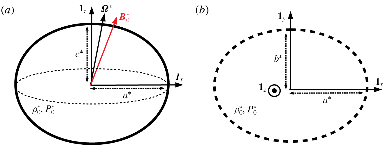
Taking into account all the physical ingredients in the mathematical model is unnecessary for MAV. We build a forward model accounting only for the key physical ingredients, namely adiabatic compressibility, rotation and the leading-order magnetic field component. As depicted in figure 1, we consider a fluid-filled rigid ellipsoid, of semi-major axes  $[a^{\ast },b^{\ast },c^{\ast }]$ and volume
 $V=4\unicode[STIX]{x03C0}a^{\ast }b^{\ast }c^{\ast }/3$. The rigid ellipsoidal cavity is rotating with the angular velocity
 $\unicode[STIX]{x1D734}^{\ast }=\unicode[STIX]{x1D6FA}_{s}^{\ast }\,\mathbf{1}_{\unicode[STIX]{x1D6FA}}$, where
 $\mathbf{1}_{\unicode[STIX]{x1D6FA}}$ is a unit vector with respect to an inertial frame. In the following, we work exclusively in the rotating frame where the boundary is steady and employ the Cartesian coordinates
 $(x^{\ast },y^{\ast },z^{\ast })$. In the rotating frame, the ellipsoidal boundary
 $\unicode[STIX]{x2202}V$ is expressed by
 $(x^{\ast }/a^{\ast })^{2}+(y^{\ast }/b^{\ast })^{2}+(z^{\ast }/c^{\ast })^{2}=1$. Moreover, the fluid can have a possible (steady) background mean flow
 $\boldsymbol{U}_{0}^{\ast }(\boldsymbol{r}^{\ast })$ (such as a differential rotation with respect to the solid-body rotation of the container, accompanied with a meridional circulation due to viscous effects), with
 $\boldsymbol{r}^{\ast }=(x^{\ast },y^{\ast },z^{\ast })^{\top }$ the position vector. This mean flow is sub-sonic for experimental conditions (yielding
 $\unicode[STIX]{x1D735}\boldsymbol{\cdot }\boldsymbol{U}_{0}^{\ast }=0$).
Sketch of the general problem. The unit Cartesian vectors are  $[\mathbf{1}_{x},\mathbf{1}_{y},\mathbf{1}_{z}]$. (a) Front view of the fluid-filled ellipsoid with (dimensional) semi-major axes
 $[a^{\ast },b^{\ast },c^{\ast }]$. (b) Top view (equatorial slice). On the boundary, the velocity satisfies the non-penetration condition.

For the sake of the numerical validation, we assume that the fluid has a spatially uniform dynamic (shear) viscosity  $\unicode[STIX]{x1D702}$, bulk viscosity
 $\unicode[STIX]{x1D702}_{B}$ and magnetic diffusivity
 $\unicode[STIX]{x1D708}_{m}$. In the theory, diffusive effects will be entirely neglected since they are often significant only in the boundary layers (Berggren et al. Reference Berggren, Bernland and Noreland2018). We also discard non-adiabatic effects to consider isentropic fluids, characterised in the reference state by the homogeneous background density
 $\unicode[STIX]{x1D70C}_{0}^{\ast }$. Within our idealised framework, we neglect gravitational effects, as well as the dynamical pressure generated by the background velocity. They are small in rotating laboratory experiments (when the flow rotation is small compared to the speed of sound). For the same reason, we also neglect centrifugal effects which are likely negligible for moderate rotation (although they could be included within our framework). Hence, the reference state has the background pressure
 $P_{0}^{\ast }$ and the speed of sound
 $C_{0}^{\ast }=\sqrt{K_{0}^{\ast }/\unicode[STIX]{x1D70C}_{0}^{\ast }}$, with
 $K_{0}^{\ast }$ the isentropic bulk modulus, that are spatially uniform. For an isentropic gas, we have
 $K_{0}^{\ast }=\unicode[STIX]{x1D6FE}P_{0}^{\ast }$ with
 $\unicode[STIX]{x1D6FE}$ the adiabatic index. The fluid is also pervaded by a background magnetic field
 $\boldsymbol{B}_{0}^{\ast }(\boldsymbol{r}^{\ast })$. The leading-order spatial component of the background magnetic field is usually the (aligned) dipole in fluid experiments, such as in the Maryland spherical Couette flow experiment (e.g. Kelley et al. Reference Kelley, Triana, Zimmerman, Tilgner and Lathrop2007) or the Derviche Tourneur Sodium (DTS) experiment (e.g. Tigrine et al. Reference Tigrine, Nataf, Schaeffer, Cardin and Plunian2019). Thus, we only retain for the background magnetic field its spatially uniform component, that is
 $\boldsymbol{B}_{0}^{\ast }=B_{0}^{\ast }\,\mathbf{1}_{B}$ with
 $B_{0}^{\ast }$ the strength of the magnetic field and
 $\mathbf{1}_{B}$ its unit direction.
We expand the velocity  $\boldsymbol{v}^{\ast }$, the density
 $\unicode[STIX]{x1D70C}^{\ast }$, the pressure
 $P^{\ast }$ and the magnetic field
 $\boldsymbol{B}^{\ast }$ as isentropic perturbations around the (steady) isentropic background state. This reads
 $$\begin{eqnarray}\displaystyle & \displaystyle \boldsymbol{v}^{\ast }(\boldsymbol{r}^{\ast },t^{\ast })=\boldsymbol{U}_{0}^{\ast }(\boldsymbol{r}^{\ast })+\boldsymbol{u}_{1}^{\ast }(\boldsymbol{r}^{\ast },t^{\ast }), & \displaystyle\end{eqnarray}$$
 $$\begin{eqnarray}\displaystyle & \displaystyle [\unicode[STIX]{x1D70C}^{\ast },P^{\ast },\boldsymbol{B}^{\ast }](\boldsymbol{r}^{\ast },t^{\ast })=[\unicode[STIX]{x1D70C}_{0}^{\ast },P_{0}^{\ast },\boldsymbol{B}_{0}^{\ast }]+[\unicode[STIX]{x1D70C}_{1}^{\ast },p_{1}^{\ast },\boldsymbol{b}_{1}^{\ast }](\boldsymbol{r}^{\ast },t^{\ast }), & \displaystyle\end{eqnarray}$$
 $$\begin{eqnarray}\displaystyle & \displaystyle \unicode[STIX]{x1D735}\boldsymbol{\cdot }\boldsymbol{U}_{0}^{\ast }=\unicode[STIX]{x1D735}\boldsymbol{\cdot }\boldsymbol{B}_{0}^{\ast }=\unicode[STIX]{x1D735}\boldsymbol{\cdot }\boldsymbol{b}_{1}^{\ast }=0. & \displaystyle\end{eqnarray}$$
 $$\begin{eqnarray}\displaystyle \frac{\unicode[STIX]{x2202}\boldsymbol{u}_{1}^{\ast }}{\unicode[STIX]{x2202}t^{\ast }}+2\,\unicode[STIX]{x1D734}^{\ast }\times \boldsymbol{u}_{1}^{\ast } & = & \displaystyle -\unicode[STIX]{x1D735}(p_{1}^{\ast }/\unicode[STIX]{x1D70C}_{0}^{\ast })+\frac{1}{\unicode[STIX]{x1D70C}_{0}^{\ast }\unicode[STIX]{x1D707}_{0}}(\unicode[STIX]{x1D735}\times \boldsymbol{b}_{1}^{\ast })\times \boldsymbol{B}_{0}^{\ast }\nonumber\\ \displaystyle & & \displaystyle -\,(\boldsymbol{U}_{0}^{\ast }\boldsymbol{\cdot }\unicode[STIX]{x1D735})\,\boldsymbol{u}_{1}^{\ast }-(\boldsymbol{u}_{1}^{\ast }\boldsymbol{\cdot }\unicode[STIX]{x1D735})\,\boldsymbol{U}_{0}^{\ast }+\unicode[STIX]{x1D708}\,\boldsymbol{f}_{v}^{\ast }(\boldsymbol{u}_{1}^{\ast }),\end{eqnarray}$$
 $$\begin{eqnarray}\displaystyle & \displaystyle \frac{\unicode[STIX]{x2202}\boldsymbol{b}_{1}^{\ast }}{\unicode[STIX]{x2202}t^{\ast }}-\unicode[STIX]{x1D735}\times (\boldsymbol{U}_{0}^{\ast }\times \boldsymbol{b}_{1}^{\ast })=\unicode[STIX]{x1D735}\times (\boldsymbol{u}_{1}^{\ast }\times \boldsymbol{B}_{0}^{\ast })+\unicode[STIX]{x1D708}_{m}\unicode[STIX]{x1D6FB}^{2}\boldsymbol{b}_{1}^{\ast }, & \displaystyle\end{eqnarray}$$
 $$\begin{eqnarray}\displaystyle & \displaystyle \frac{\unicode[STIX]{x2202}\unicode[STIX]{x1D70C}_{1}^{\ast }}{\unicode[STIX]{x2202}t^{\ast }}+\boldsymbol{U}_{0}^{\ast }\boldsymbol{\cdot }\unicode[STIX]{x1D735}\unicode[STIX]{x1D70C}_{1}^{\ast }=-\unicode[STIX]{x1D70C}_{0}^{\ast }\,\unicode[STIX]{x1D735}\boldsymbol{\cdot }\boldsymbol{u}_{1}^{\ast }, & \displaystyle\end{eqnarray}$$
 $\unicode[STIX]{x1D707}_{0}$ the magnetic permeability of the vacuum,
 $\unicode[STIX]{x1D708}=\unicode[STIX]{x1D702}/\unicode[STIX]{x1D70C}_{0}^{\ast }$ the kinematic viscosity, the viscous force
 $$\begin{eqnarray}\boldsymbol{f}_{v}^{\ast }(\boldsymbol{u}_{1}^{\ast })=\unicode[STIX]{x1D6FB}^{2}\boldsymbol{u}_{1}^{\ast }+\left(\frac{1}{3}+\frac{\unicode[STIX]{x1D708}_{B}}{\unicode[STIX]{x1D708}}\right)\unicode[STIX]{x1D735}(\unicode[STIX]{x1D735}\boldsymbol{\cdot }\boldsymbol{u}_{1}^{\ast })\end{eqnarray}$$
and the bulk kinematic viscosity  $\unicode[STIX]{x1D708}_{B}=\unicode[STIX]{x1D702}_{B}/\unicode[STIX]{x1D70C}_{0}^{\ast }$. The governing equation for the pressure is obtained by using the equation of state for an isentropic fluid. We get
 $$\begin{eqnarray}\frac{\unicode[STIX]{x2202}p_{1}^{\ast }}{\unicode[STIX]{x2202}t^{\ast }}+\boldsymbol{U}_{0}^{\ast }\boldsymbol{\cdot }\unicode[STIX]{x1D735}p_{1}^{\ast }=-\unicode[STIX]{x1D70C}_{0}^{\ast }{C_{0}^{\ast }}^{2}\,\unicode[STIX]{x1D735}\boldsymbol{\cdot }\boldsymbol{u}_{1}^{\ast }.\end{eqnarray}$$
Finally, equations (2.2) are supplemented with boundary conditions. The velocity satisfies the non-penetration (Dirichlet) condition on the rigid ellipsoidal wall  $\boldsymbol{u}_{1}^{\ast }\boldsymbol{\cdot }\mathbf{1}_{n}=0$, where
 $\mathbf{1}_{n}$ is the unit vector normal to the boundary. In addition to the non-penetration condition, diffusive and pressure boundary conditions will be enforced in the diffusive numerical computations that will be used for the validation (see appendix A). However, no additional boundary condition is required in the diffusionless theory.
2.2 Dimensionless variables
For the numerical convenience, we work in dimensionless variables. We use the semi-major axis  $a^{\ast }$ as length scale,
 $a^{\ast }/C_{0}^{\ast }$ as time scale,
 $\unicode[STIX]{x1D70C}_{0}^{\ast }$ as density scale and
 $\unicode[STIX]{x1D70C}_{0}^{\ast }{C_{0}^{\ast }}^{2}$ as pressure scale. We choose the typical amplitude
 $B_{0}^{\ast }$ of the dimensional background magnetic field as magnetic scale. We also introduce the typical amplitude of the background velocity field
 $U_{0}^{\ast }$. The dimensionless fields are written without an asterisk, to distinguish them from their dimensional counterparts. Then, equations (2.2)–(2.4) read in dimensionless form
 $$\begin{eqnarray}\displaystyle \frac{\unicode[STIX]{x2202}\boldsymbol{u}_{1}}{\unicode[STIX]{x2202}t}+2M_{\unicode[STIX]{x1D6FA}}\,\mathbf{1}_{\unicode[STIX]{x1D6FA}}\times \boldsymbol{u}_{1} & = & \displaystyle -\unicode[STIX]{x1D735}p_{1}+M_{A}^{2}(\unicode[STIX]{x1D735}\times \boldsymbol{b}_{1})\times \mathbf{1}_{B}\nonumber\\ \displaystyle & & \displaystyle -\,M_{S}[(\boldsymbol{U}_{0}\boldsymbol{\cdot }\unicode[STIX]{x1D735})\boldsymbol{u}_{1}+(\boldsymbol{u}_{1}\boldsymbol{\cdot }\unicode[STIX]{x1D735})\boldsymbol{U}_{0}]+Re_{S}^{-1}\,\boldsymbol{f}_{v}(\boldsymbol{u}_{1}),\end{eqnarray}$$
 $$\begin{eqnarray}\displaystyle & \displaystyle \frac{\unicode[STIX]{x2202}p_{1}}{\unicode[STIX]{x2202}t}+M_{S}(\boldsymbol{U}_{0}\boldsymbol{\cdot }\unicode[STIX]{x1D735}p_{1})=-\unicode[STIX]{x1D735}\boldsymbol{\cdot }\boldsymbol{u}_{1}, & \displaystyle\end{eqnarray}$$
 $$\begin{eqnarray}\displaystyle & \displaystyle \frac{\unicode[STIX]{x2202}\boldsymbol{b}_{1}}{\unicode[STIX]{x2202}t}-M_{S}\,\unicode[STIX]{x1D735}\times (\boldsymbol{U}_{0}\times \boldsymbol{b}_{1})=\unicode[STIX]{x1D735}\times (\boldsymbol{u}_{1}\times \mathbf{1}_{B})+Rm_{S}^{-1}\,\unicode[STIX]{x1D6FB}^{2}\boldsymbol{b}_{1}. & \displaystyle\end{eqnarray}$$
 $$\begin{eqnarray}M_{S}=\frac{U_{0}^{\ast }}{C_{0}^{\ast }},\quad M_{\unicode[STIX]{x1D6FA}}=\frac{a^{\ast }\unicode[STIX]{x1D6FA}_{s}^{\ast }}{C_{0}^{\ast }}\quad \text{and}\quad M_{A}=\frac{V_{A}^{\ast }}{C_{0}^{\ast }},\end{eqnarray}$$
where  $V_{A}^{\ast }=B_{0}^{\ast }/\sqrt{\unicode[STIX]{x1D70C}_{0}^{\ast }\unicode[STIX]{x1D707}_{0}}$ is the Alfvén velocity. They compare the typical time scales for the flow, rotation and the magnetic field with the sonic time scale. Note that
 $M_{S}$ can be negative, if the background flow is retrograde compared to global rotation. We can also define (for rotating flows only) the Rossby number
 $Ro=M_{S}/M_{\unicode[STIX]{x1D6FA}}$, which measures the strength of the background mean flow compared to global rotation. The diffusive effects are quantified by the sonic Reynolds and magnetic Reynolds numbers (based on the speed of sound), defined as
 $$\begin{eqnarray}Re_{S}=\frac{C_{0}^{\ast }a^{\ast }}{\unicode[STIX]{x1D708}}\quad \text{and}\quad Rm_{S}=\frac{C_{0}^{\ast }a^{\ast }}{\unicode[STIX]{x1D708}_{m}}.\end{eqnarray}$$
In the presence of global rotation, we can also introduce the Ekman number  $Ek=\unicode[STIX]{x1D708}/(\unicode[STIX]{x1D6FA}_{s}^{\ast }{a^{\ast }}^{2})$. Finally,
 $M_{A}$ is related in rotating magnetohydrodynamics to the Lehnert number
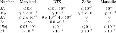
 $Le=M_{A}/M_{\unicode[STIX]{x1D6FA}}$. The typical values of these numbers in experiments are given in table 1. Their magnitudes will allow us to simplify the theory of the compressible modes. Finally, given the high accuracy of typical acoustic measurements (e.g. Su et al. Reference Su, Cébron, Nataf, Cardin, Vidal, Solazzo and Do2020), note that we must be able to resolve frequency variations as small as 10-4–10-3 in dimensionless units.
Typical values of the dimensionless numbers for laboratory experiments in spherical-like domains. Maryland experiment: Kelley et al. (Reference Kelley, Triana, Zimmerman, Tilgner and Lathrop2007), Rieutord et al. (Reference Rieutord, Triana, Zimmerman and Lathrop2012), Triana et al. (Reference Triana, Zimmerman, Nataf, Thorette, Lekic and Lathrop2014) and Zimmerman et al. (Reference Zimmerman, Triana, Nataf and Lathrop2014). DTS experiment: Figueroa et al. (Reference Figueroa, Schaeffer, Nataf and Schmitt2013) and Tigrine et al. (Reference Tigrine, Nataf, Schaeffer, Cardin and Plunian2019). ZoRo experiment: Su et al. (Reference Su, Cébron, Nataf, Cardin, Vidal, Solazzo and Do2020). Marseille ellipsoidal experiments: Grannan et al. (Reference Grannan, Favier, Le Bars and Aurnou2016), Lemasquerier et al. (Reference Lemasquerier, Grannan, Vidal, Cébron, Favier, Le Bars and Aurnou2017) and Le Reun et al. (Reference Le Reun, Favier and Le Bars2019).

2.3 Master wave-like equation
We are now in a position to build the wave-like equation of the rotating magneto-acoustic modes in rigid ellipsoids. We leave aside diffusive and non-adiabatic effects. Indeed, (rapidly) rotating fluid experiments are usually characterised by small diffusive effects (except possibly in the thin boundary layers, see Berggren et al. (Reference Berggren, Bernland and Noreland2018)), that is  $Re_{S}\gg 1$ (or
 $Ek\ll 1$ with rotation) in table 1. They can (often) be considered as small perturbations of the diffusionless modes (e.g. Moldover et al. Reference Moldover, Mehl and Greenspan1986). We can recast diffusionless primitive equations (2.5) into a wave-like equation for the fluid particle displacement vector
 $\unicode[STIX]{x1D743}_{1}(\boldsymbol{r},t)$. This is a prerequisite to obtain the frequency shift of the modes generated by the background mean flow (e.g. Aerts et al. Reference Aerts, Christensen-Dalsgaard and Kurtz2010). The Eulerian velocity perturbation is related to
 $\unicode[STIX]{x1D743}_{1}$ by (e.g. Lynden-Bell & Ostriker Reference Lynden-Bell and Ostriker1967)
 $$\begin{eqnarray}\boldsymbol{u}_{1}=\frac{\unicode[STIX]{x2202}\unicode[STIX]{x1D743}_{1}}{\unicode[STIX]{x2202}t}+(\boldsymbol{U}_{0}\boldsymbol{\cdot }\unicode[STIX]{x1D735})\unicode[STIX]{x1D743}_{1}-(\unicode[STIX]{x1D743}_{1}\boldsymbol{\cdot }\unicode[STIX]{x1D735})\boldsymbol{U}_{0}.\end{eqnarray}$$
We also obtain from pressure and induction equations in dimensionless units (e.g. Bernstein et al. Reference Bernstein, Frieman, Kruskal and Kulsrud1958; Frieman & Rotenberg Reference Frieman and Rotenberg1960)
 $$\begin{eqnarray}p_{1}=-\unicode[STIX]{x1D735}\boldsymbol{\cdot }\unicode[STIX]{x1D743}_{1},\quad \boldsymbol{b}_{1}=\unicode[STIX]{x1D735}\times (\unicode[STIX]{x1D743}_{1}\times \mathbf{1}_{B}).\end{eqnarray}$$
Now, we substitute (2.8)–(2.9) into momentum equation (2.2a), yielding the (dimensionless) master wave-like equation for the displacement vector
 $$\begin{eqnarray}\frac{\unicode[STIX]{x2202}^{2}\unicode[STIX]{x1D743}_{1}}{\unicode[STIX]{x2202}t^{2}}+\boldsymbol{{\mathcal{C}}}\left(\frac{\unicode[STIX]{x2202}\unicode[STIX]{x1D743}_{1}}{\unicode[STIX]{x2202}t}\right)+\boldsymbol{{\mathcal{K}}}(\unicode[STIX]{x1D743}_{1})=\mathbf{0},\quad \unicode[STIX]{x1D743}_{1}\boldsymbol{\cdot }\mathbf{1}_{n}=0\quad \text{on}~\unicode[STIX]{x2202}V,\end{eqnarray}$$
with the linear operators
 $$\begin{eqnarray}\displaystyle \boldsymbol{{\mathcal{C}}}(\unicode[STIX]{x1D743}_{1})=2\,\mathbf{1}_{\unicode[STIX]{x1D6FA}}\times \unicode[STIX]{x1D743}_{1}+2M_{S}\,(\boldsymbol{U}_{0}\boldsymbol{\cdot }\unicode[STIX]{x1D735})\,\unicode[STIX]{x1D743}_{1}, & & \displaystyle\end{eqnarray}$$
 $$\begin{eqnarray}\displaystyle \boldsymbol{{\mathcal{K}}}(\unicode[STIX]{x1D743}_{1}) & = & \displaystyle M_{S}^{2}(\boldsymbol{U}_{0}\boldsymbol{\cdot }\unicode[STIX]{x1D735})^{2}\unicode[STIX]{x1D743}_{1}+2M_{\unicode[STIX]{x1D6FA}}M_{S}\,\mathbf{1}_{\unicode[STIX]{x1D6FA}}\times (\boldsymbol{U}_{0}\boldsymbol{\cdot }\unicode[STIX]{x1D735}\unicode[STIX]{x1D743}_{1})-\unicode[STIX]{x1D735}[\unicode[STIX]{x1D735}\boldsymbol{\cdot }\unicode[STIX]{x1D743}_{1}]\nonumber\\ \displaystyle & & \displaystyle -\,\unicode[STIX]{x1D743}_{1}\boldsymbol{\cdot }\unicode[STIX]{x1D735}[2M_{\unicode[STIX]{x1D6FA}}M_{S}\,\mathbf{1}_{\unicode[STIX]{x1D6FA}}\times \boldsymbol{U}_{0}+M_{S}^{2}(\boldsymbol{U}_{0}\boldsymbol{\cdot }\unicode[STIX]{x1D735})\boldsymbol{U}_{0}]\nonumber\\ \displaystyle & & \displaystyle -\,M_{A}^{2}[\unicode[STIX]{x1D735}\times \unicode[STIX]{x1D735}\times (\unicode[STIX]{x1D743}_{1}\times \mathbf{1}_{B})]\times \mathbf{1}_{B}.\end{eqnarray}$$
 $\boldsymbol{{\mathcal{C}}}$ is skew–Hermitian (Lynden-Bell & Ostriker Reference Lynden-Bell and Ostriker1967), whereas operator
 $\boldsymbol{{\mathcal{K}}}$ is Hermitian without considering our chosen background magnetic field. Finally, we seek modal solutions
 $$\begin{eqnarray}\unicode[STIX]{x1D743}_{1}(\boldsymbol{r},t)=\unicode[STIX]{x1D743}(\boldsymbol{r})\exp (\unicode[STIX]{x1D706}t),\quad \unicode[STIX]{x1D743}\boldsymbol{\cdot }\mathbf{1}_{n}=0\quad \text{on}~\unicode[STIX]{x2202}V,\end{eqnarray}$$
where  $\unicode[STIX]{x1D706}=\unicode[STIX]{x1D70E}+\text{i}\unicode[STIX]{x1D714}$ is the (complex-valued) eigenvalue with the decay (or growth) rate
 $\unicode[STIX]{x1D70E}\in \mathbb{R}$ and the angular frequency
 $\unicode[STIX]{x1D714}\in \mathbb{R}$. Then, problem (2.11) reduces to the quadratic eigenvalue problem
 $$\begin{eqnarray}\unicode[STIX]{x1D706}^{2}\unicode[STIX]{x1D743}+\unicode[STIX]{x1D706}\,\boldsymbol{{\mathcal{C}}}(\unicode[STIX]{x1D743})+\boldsymbol{{\mathcal{K}}}(\unicode[STIX]{x1D743})=\mathbf{0},\quad \unicode[STIX]{x1D743}\boldsymbol{\cdot }\mathbf{1}_{n}=0\quad \text{on}~\unicode[STIX]{x2202}V.\end{eqnarray}$$
MAV consists in reconciling predictions obtained by solving (2.13) with the observed acoustic spectrum, to retrieve the (unknown) background flow.
3 Polynomial spectral method
We introduce the mathematical result of the paper, that is the new polynomial spectral method in rigid ellipsoids. We will apply it to solve magneto-acoustic problem (2.13). Yet, a wide class of linear problems in (rigid) ellipsoids is readily amenable to the attack presented below. For instance, the hydromagnetic modes (e.g. Vidal et al. Reference Vidal, Cébron, ud Doula and Alecian2019) or various orbitally driven instabilities (e.g. Kerswell Reference Kerswell1993, Reference Kerswell2002; Vantieghem et al. Reference Vantieghem, Cébron and Noir2015; Vidal & Cébron Reference Vidal and Cébron2017) can be considered for incompressible fluids. Thus, the polynomial method for compressible flows is worth presenting in general terms. In the rotating frame, we consider the canonical linear problem for a vector field  $\boldsymbol{u}$ bounded in a rigid ellipsoid
 $$\begin{eqnarray}\boldsymbol{{\mathcal{M}}}\left(\frac{\unicode[STIX]{x2202}^{2}\boldsymbol{u}}{\unicode[STIX]{x2202}t^{2}}\right)+\boldsymbol{{\mathcal{C}}}\left(\frac{\unicode[STIX]{x2202}\boldsymbol{u}}{\unicode[STIX]{x2202}t}\right)+\boldsymbol{{\mathcal{K}}}(\boldsymbol{u})=\mathbf{0}\quad \text{in}~V,\quad \boldsymbol{u}\boldsymbol{\cdot }\mathbf{1}_{n}=0\quad \text{on}~\unicode[STIX]{x2202}V,\end{eqnarray}$$
where  $[\boldsymbol{{\mathcal{M}}},\boldsymbol{{\mathcal{C}}},\boldsymbol{{\mathcal{K}}}]$ are three differential operators. Problem (3.1) is equipped with the usual inner product
 $$\begin{eqnarray}\langle \boldsymbol{u},\boldsymbol{v}\rangle =\int _{V}\boldsymbol{u}^{\dagger }\boldsymbol{\cdot }\boldsymbol{v}\,\text{d}V,\end{eqnarray}$$
where  $^{\dagger }$ denotes the complex conjugate. We can reasonably approximate solutions of (3.1) by using finite-dimensional functional spaces, made of polynomial elements which are square integrable and infinitely differentiable. A similar approach has been pursed in the pioneering work of Lebovitz (Reference Lebovitz1989) for free-surface flows. We present the spectral decomposition for rigid ellipsoids in § 3.1, its polynomial expansion in § 3.2 and discuss its application to boundary-value problem (3.1) in § 3.3.
3.1 Spectral decomposition
Assuming that  $\boldsymbol{u}$ is square integrable and (at least) two-times continuously differentiable in (3.1), we expand
 $\boldsymbol{u}$ by using the Helmholtz–Hodge decomposition. This reads
 $$\begin{eqnarray}\boldsymbol{u}=\unicode[STIX]{x1D735}\unicode[STIX]{x1D6F7}+\unicode[STIX]{x1D735}\times \unicode[STIX]{x1D733},\quad \boldsymbol{u}\boldsymbol{\cdot }\mathbf{1}_{n}=0\quad \text{on}~\unicode[STIX]{x2202}V,\end{eqnarray}$$
with  $\unicode[STIX]{x1D6F7}$ the scalar potential and
 $\unicode[STIX]{x1D733}$ the vector potential. The two components
 $\unicode[STIX]{x1D735}\unicode[STIX]{x1D6F7}$ and
 $\unicode[STIX]{x1D735}\times \unicode[STIX]{x1D733}$ are orthogonal with respect to inner product (3.2). The potentials are found by solving the following problems
 $$\begin{eqnarray}\left.\begin{array}{@{}ll@{}}\unicode[STIX]{x1D6FB}^{2}\unicode[STIX]{x1D6F7}=\unicode[STIX]{x1D735}\boldsymbol{\cdot }\boldsymbol{ u} & \text{in}~V,\\ \unicode[STIX]{x1D735}\unicode[STIX]{x1D6F7}\boldsymbol{\cdot }\mathbf{1}_{n}=0 & \text{on}~\unicode[STIX]{x2202}V,\end{array}\right\}\quad \left.\begin{array}{@{}ll@{}}\unicode[STIX]{x1D735}\times (\unicode[STIX]{x1D735}\times \unicode[STIX]{x1D733})=\unicode[STIX]{x1D735}\times \boldsymbol{u} & \text{in}~V,\\ (\unicode[STIX]{x1D735}\times \unicode[STIX]{x1D733})\boldsymbol{\cdot }\mathbf{1}_{n}=0 & \text{on}~\unicode[STIX]{x2202}V.\end{array}\right\}\end{eqnarray}$$
Solutions of Neumann problem (3.4) for the scalar potential are usually written as the sum of homogeneous and particular potentials  $\unicode[STIX]{x1D6F7}=\unicode[STIX]{x1D6F7}_{u}+\unicode[STIX]{x1D6F7}_{w}$, such that
 $$\begin{eqnarray}\unicode[STIX]{x1D6FB}^{2}\unicode[STIX]{x1D6F7}_{u}=0,\quad \unicode[STIX]{x1D6FB}^{2}\unicode[STIX]{x1D6F7}_{w}=\unicode[STIX]{x1D735}\boldsymbol{\cdot }\boldsymbol{u}.\end{eqnarray}$$
Non-trivial solutions  $\unicode[STIX]{x1D6F7}_{u}\neq 0$ only exist when the normal component of
 $\boldsymbol{u}$ does not vanish on some part of the boundary (Kellog Reference Kellog1953). Hence, we have
 $\unicode[STIX]{x1D6F7}_{u}=0$ in rigid ellipsoids (e.g. Backus & Rieutord Reference Backus and Rieutord2017). Therefore, any vector
 $\boldsymbol{u}$ bounded in rigid ellipsoids lies in the union of two orthogonal linear vector spaces
 $\boldsymbol{{\mathcal{V}}}\oplus \boldsymbol{{\mathcal{W}}}$, such that
 $$\begin{eqnarray}\displaystyle & \displaystyle \boldsymbol{{\mathcal{V}}}:\{\boldsymbol{e}=\unicode[STIX]{x1D735}\times \unicode[STIX]{x1D733},\unicode[STIX]{x1D735}\boldsymbol{\cdot }\boldsymbol{e}=0,\boldsymbol{e}\boldsymbol{\cdot }\mathbf{1}_{n}=0~\text{on}~\unicode[STIX]{x2202}V\}, & \displaystyle\end{eqnarray}$$
 $$\begin{eqnarray}\displaystyle & \displaystyle \boldsymbol{{\mathcal{W}}}:\{\boldsymbol{e}=\unicode[STIX]{x1D735}\unicode[STIX]{x1D6F7}_{w},~\boldsymbol{e}\boldsymbol{\cdot }\mathbf{1}_{n}=0~\text{on}~\unicode[STIX]{x2202}V\}. & \displaystyle\end{eqnarray}$$
 $\unicode[STIX]{x1D6F7}_{u}\neq 0$ (e.g. Lebovitz Reference Lebovitz1989). The associated decomposition for the scalar
 $\unicode[STIX]{x1D6F7}_{u}$ has been employed in acoustics by Vidal, Su & Cébron (Reference Vidal, Su and Cébron2019b).
3.2 Polynomial vector spaces
We introduce the finite-dimensional space  ${\mathcal{P}}\,[l,l]$, spanned by all Cartesian monomials
 $x^{i}y^{j}z^{k}$ of degree
 $i+j+k=l$. Its dimension is
 $\dim {\mathcal{P}}\,[l,l]=(l+1)(l+2)/2$ (e.g. Backus & Rieutord Reference Backus and Rieutord2017). We denote
 ${\mathcal{P}}\,[0,n]$ the finite-dimensional space of all polynomial scalars of degree
 $i+j+k\leqslant n$. We now define the finite-dimensional space
 $\boldsymbol{{\mathcal{P}}}\,[0,n]$ of all polynomial vectors for which each component, belonging to
 ${\mathcal{P}}\,[0,n]$, is made of Cartesian monomials
 $x^{i}y^{j}z^{k}$ (of maximum degree
 $i+j+k\leqslant n$). Its dimension is
 $\dim \boldsymbol{{\mathcal{P}}}\,[0,n]=(n+1)(n+2)(n+3)/2$ (e.g. Lebovitz Reference Lebovitz1989; Backus & Rieutord Reference Backus and Rieutord2017). It is known that any two-times continuously differentiable field appearing in (3.1) can be uniformly approximated by Cartesian polynomials belonging to
 $\boldsymbol{{\mathcal{P}}}\,[0,n]$ (Weierstrass approximation theorem). This polynomial decomposition has proven useful for free-surface flows in astrophysics (e.g. Chandrasekhar Reference Chandrasekhar1969), and has been rediscovered in elasticity (e.g. Visscher et al. Reference Visscher, Migliori, Bell and Reinert1991; Saviot & Murray Reference Saviot and Murray2009). However, these polynomial elements do not naturally satisfy the rigid boundary condition (contrary to the ones introduced below).
Instead, we restrict the vector space  $\boldsymbol{{\mathcal{V}}}\oplus \boldsymbol{{\mathcal{W}}}$ to the finite-dimensional space
 $\boldsymbol{{\mathcal{P}}}\,[0,n]$, by considering basis elements in
 $\boldsymbol{{\mathcal{P}}}\,[0,n]$ that satisfy the non-penetration condition. The quest for a polynomial description of
 $\boldsymbol{{\mathcal{V}}}\oplus \boldsymbol{{\mathcal{W}}}$ hinges on the facts that (i) the ellipsoid is a smooth quadratic surface in Cartesian coordinates (
 $\mathbf{1}_{n}$ is a polynomial vector) and that (ii) some modes supported by (2.10) admit polynomial solutions (e.g. Vantieghem Reference Vantieghem2014; Backus & Rieutord Reference Backus and Rieutord2017). We define the restrictions of
 $[\boldsymbol{{\mathcal{V}}},\boldsymbol{{\mathcal{W}}}]$ to the finite-dimensional polynomial vector space
 $\boldsymbol{{\mathcal{P}}}\,[0,n]$, denoted
 $\boldsymbol{{\mathcal{V}}}\,[0,n]\subset \boldsymbol{{\mathcal{P}}}\,[0,n]$ and
 $\boldsymbol{{\mathcal{W}}}\,[0,n]\subset \boldsymbol{{\mathcal{P}}}\,[0,n]$. We have
 $\dim \boldsymbol{{\mathcal{V}}}\,[0,n]<\dim \boldsymbol{{\mathcal{P}}}\,[0,n]$ and
 $\dim \boldsymbol{{\mathcal{W}}}\,[0,n]<\dim \boldsymbol{{\mathcal{P}}}\,[0,n]$. We build polynomial basis vectors for
 $\boldsymbol{{\mathcal{V}}}\,[0,n]$ and
 $\boldsymbol{{\mathcal{W}}}\,[0,n]$, involving linear combinations of Cartesian monomials
 $x^{i}y^{j}z^{k}$ (of maximum degree
 $i+j+k\leqslant n$) that satisfy the non-penetration condition, as follows.
3.2.1 Basis for  $\boldsymbol{{\mathcal{V}}}\,[0,n]$

Divergenceless fields represented by the potential vector  $\unicode[STIX]{x1D733}$ in decomposition (3.6a) can be described by two scalar fields, denoted
 $[{\mathcal{A}},{\mathcal{B}}]$ in the following. Various descriptions for these scalars have been be proposed, for instance based on different forms of poloidal/toroidal-like decompositions (e.g. Gledzer & Ponomarev Reference Gledzer and Ponomarev1992; Wu & Roberts Reference Wu and Roberts2011; Ivers Reference Ivers2017). Instead, we define
 $[{\mathcal{A}},{\mathcal{B}}]$ as Clebsch (or Euler) scalars. Then, the spectral decomposition for
 $\boldsymbol{e}\in \boldsymbol{{\mathcal{V}}}$ simplifies into
 $$\begin{eqnarray}\boldsymbol{e}=\unicode[STIX]{x1D735}\times ({\mathcal{A}}\unicode[STIX]{x1D735}{\mathcal{B}})=\unicode[STIX]{x1D735}{\mathcal{A}}\times \unicode[STIX]{x1D735}{\mathcal{B}}.\end{eqnarray}$$
This decomposition has also been introduced to describe quasi-geostrophic motions, almost invariant along the rotation axis (e.g. in spheres Labbé, Jault & Gillet Reference Labbé, Jault and Gillet2015). Decomposition (3.7) is of practical interest, since the non-penetration condition is automatically satisfied if either  ${\mathcal{A}}$ or
 ${\mathcal{B}}$ is constant on the boundary
 $\unicode[STIX]{x2202}V$. Lebovitz (Reference Lebovitz1989) found admissible polynomial bases for the scalars
 $[{\mathcal{A}},{\mathcal{B}}]$ as follows.
We consider the linearly independent Cartesian monomials in  ${\mathcal{P}}\,[0,n-1]$, that is
 $x^{i}y^{j}z^{k}$ with
 $i+i+k\leqslant n-1$. Their number is
 $N_{2}=n(n+1)(n+2)/6$. Among them, there are
 $N_{1}=n(n+1)/2$ monomials that are independent of
 $z$, denoted
 $\mathfrak{g}_{i}$. The other monomials, denoted
 $\mathfrak{h}_{i}$, contain
 $z$ as factor. We index the set of these polynomials as
 $$\begin{eqnarray}\displaystyle & \displaystyle \{\mathfrak{g}_{i}\}=\{1,x,y,x^{2},xy,y^{2},\ldots ,x^{n-1},y^{n-1}\},\quad i\in [1,N_{1}], & \displaystyle\end{eqnarray}$$
 $$\begin{eqnarray}\displaystyle & \displaystyle \{\mathfrak{h}_{i}\}=\{z,xz,yz,z^{2},\ldots ,z^{n-1}\},\quad i\in [N_{1}+1,N_{2}], & \displaystyle\end{eqnarray}$$
 $\{\mathfrak{p}_{i}\}=\{\mathfrak{g}_{i}\}\,\bigcup \,\{\mathfrak{h}_{i}\}$ with
 $i\in [1,N_{2}]$. Then, we define the three pairs of Clebsch scalars (e.g. Lebovitz Reference Lebovitz1989)
 $$\begin{eqnarray}\displaystyle & \displaystyle \{{\mathcal{A}}=\mathfrak{p}_{i}F,{\mathcal{B}}=x\}\quad \text{with}~i\in [1,N_{2}]\quad \Rightarrow \quad \boldsymbol{e}_{i}=\unicode[STIX]{x1D735}[\mathfrak{p}_{i}F]\times \mathbf{1}_{x}, & \displaystyle\end{eqnarray}$$
 $$\begin{eqnarray}\displaystyle & \displaystyle \{{\mathcal{A}}=\mathfrak{p}_{i}F,{\mathcal{B}}=y\}\quad \text{with}~i\in [1,N_{2}]\quad \Rightarrow \quad \boldsymbol{e}_{N_{2}+i}=\unicode[STIX]{x1D735}[\mathfrak{p}_{i}F]\times \mathbf{1}_{y}, & \displaystyle\end{eqnarray}$$
 $$\begin{eqnarray}\displaystyle & \displaystyle \{{\mathcal{A}}=\mathfrak{g}_{i}F,{\mathcal{B}}=z\}\quad \text{with}~i\in [1,N_{1}]\quad \Rightarrow \quad \boldsymbol{e}_{2N_{2}+i}=\unicode[STIX]{x1D735}[\mathfrak{g}_{i}F]\times \mathbf{1}_{z}, & \displaystyle\end{eqnarray}$$
 $F=1-(x/a)^{2}-(y/b)^{2}-(z/c)^{2}$. The enumeration of these elements gives the dimension of
 $\boldsymbol{{\mathcal{V}}}\,[0,n]$ (see also Backus & Rieutord (Reference Backus and Rieutord2017))
 $$\begin{eqnarray}\dim \boldsymbol{{\mathcal{V}}}\,[0,n]=N_{1}+2N_{2}=n(n+1)(2n+7)/6.\end{eqnarray}$$
Hence,  $\boldsymbol{{\mathcal{V}}}\,[0,0]$ is empty and the polynomial elements of
 $\boldsymbol{{\mathcal{V}}}\,[0,n]$ are at least linear in the Cartesian coordinates. Polynomial elements (3.9) are linearly independent (Lebovitz Reference Lebovitz1989). They are neither normalised nor (fully) orthogonal, but they can be orthonormalised with the (modified) Gram–Schmidt algorithm.
3.2.2 Basis for $\boldsymbol{{\mathcal{W}}}\,[0,n]$

In investigating the properties of the inertial modes, Cartan (Reference Cartan1922) outlined an algorithm to build the elements  $\boldsymbol{e}=\unicode[STIX]{x1D735}\unicode[STIX]{x1D6F7}_{w}\in \boldsymbol{{\mathcal{W}}}\,[0,n]$ in ellipsoidal coordinates. Yet, they admit much simpler explicit expressions in Cartesian coordinates. We introduce the (non-normalised) normal gradient operator
 ${\mathcal{N}}$, defined by
 $$\begin{eqnarray}{\mathcal{N}}=\boldsymbol{n}\boldsymbol{\cdot }\unicode[STIX]{x1D735}=\frac{x}{a^{2}}\frac{\unicode[STIX]{x2202}}{\unicode[STIX]{x2202}x}+\frac{y}{b^{2}}\frac{\unicode[STIX]{x2202}}{\unicode[STIX]{x2202}y}+\frac{z}{c^{2}}\frac{\unicode[STIX]{x2202}}{\unicode[STIX]{x2202}z},\end{eqnarray}$$
with  $\boldsymbol{n}=(x/a^{2},y/b^{2},z/c^{2})^{\top }$. For a given monomial
 $x^{i}y^{j}z^{k}\in {\mathcal{P}}\,[1,n+1]$, we have
 $$\begin{eqnarray}{\mathcal{N}}(x^{i}y^{j}z^{k})=\left(\frac{i}{a^{2}}+\frac{j}{b^{2}}+\frac{k}{c^{2}}\right)x^{i}y^{j}z^{k}.\end{eqnarray}$$
Since  $i+j+k\geqslant 1$, we can obtain the inverse operator
 ${\mathcal{N}}^{-1}$ such that
 ${\mathcal{N}}^{-1}{\mathcal{N}}(x^{i}y^{j}z^{k})=x^{i}y^{j}z^{k}$, yielding
 $$\begin{eqnarray}{\mathcal{N}}^{-1}=\frac{1}{(i/a^{2}+j/b^{2}+k/c^{2})^{2}}\,{\mathcal{N}}\end{eqnarray}$$
and  ${\mathcal{N}}^{-1}(x^{i}y^{j}z^{k})=x^{i}y^{j}z^{k}/[i/a^{2}+j/b^{2}+k/c^{2}]$ for each Cartesian monomial.
Any polynomial element  $\boldsymbol{e}=\unicode[STIX]{x1D735}\unicode[STIX]{x1D6F7}_{w}\in \boldsymbol{{\mathcal{W}}}\,[0,n]$ is then expressed as a function of the polynomial scalar potential
 $\unicode[STIX]{x1D6F7}_{w}$ defined by
 $$\begin{eqnarray}\unicode[STIX]{x1D6F7}_{w}={\mathcal{N}}^{-1}(F\unicode[STIX]{x1D6F9}_{w}),\quad F=1-(x/a)^{2}-(y/b)^{2}-(z/c)^{2},\end{eqnarray}$$
with  $\unicode[STIX]{x1D6F9}_{w}\in {\mathcal{P}}\,[1,n-1]$. We have
 $\dim \boldsymbol{{\mathcal{W}}}\,[0,0]=\dim \boldsymbol{{\mathcal{W}}}\,[0,1]=0$ and, for
 $n\geqslant 2$, the one of
 ${\mathcal{P}}\,[1,n-1]$. Thus, we get
 $$\begin{eqnarray}\dim \boldsymbol{{\mathcal{W}}}\,[0,n]=n(n+1)(n+2)/6-1.\end{eqnarray}$$
Elements  $\boldsymbol{e}\in \boldsymbol{{\mathcal{W}}}\,[0,n]$ involve at least quadratic products in the Cartesian coordinates. These elements are neither normalised nor orthogonal, but they can be orthonormalised with the (modified) Gram–Schmidt algorithm. Two elements in
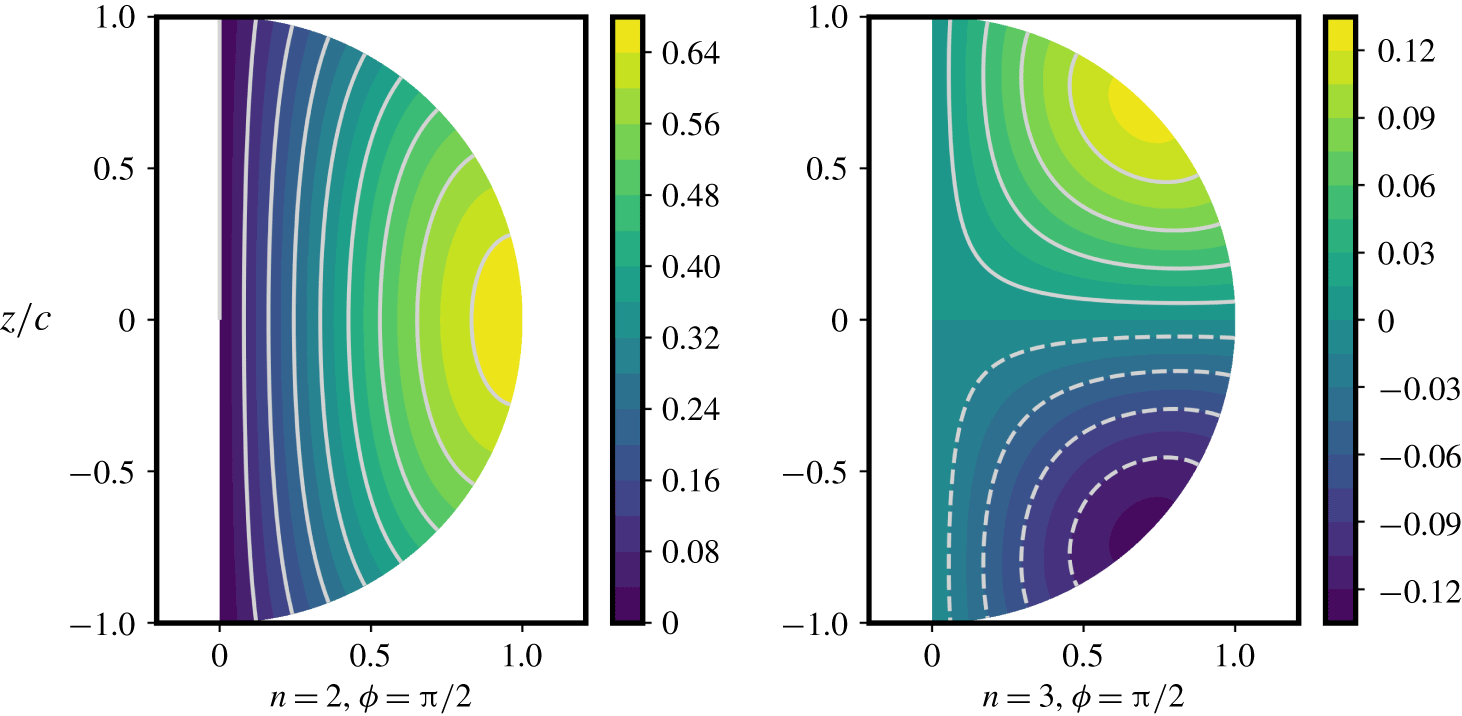
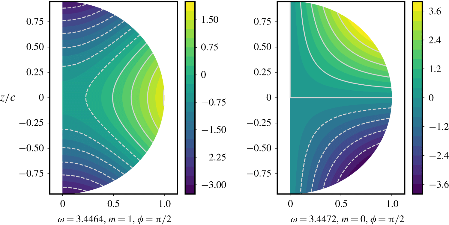
 $\boldsymbol{{\mathcal{W}}}\,[0,3]$ are illustrated in figure 2.
Meridional sections of  $\unicode[STIX]{x1D6F7}_{w}$ for the potential basis elements
 $\unicode[STIX]{x1D735}\unicode[STIX]{x1D6F7}_{w}\in \boldsymbol{{\mathcal{W}}}\,[0,3]$ in an oblate spheroid (
 $a=b=1,c=0.9$). Each section is taken in a meridional plane containing the
 $z$-axis, at the longitude
 $\unicode[STIX]{x1D719}$ measured from the long
 $x$-axis. Horizontal axis shows
 $\sqrt{x^{2}+y^{2}}$ at the longitude
 $\unicode[STIX]{x1D719}$. Colour bar shows the scalar potential
 $\unicode[STIX]{x1D6F7}_{w}$. Solid grey lines are positive iso-contours, whereas dashed grey lines represent negative iso-contours.

3.3 Method of weighted residuals
Equipped with the previous mathematical results, we develop the new global spectral method in ellipsoids for generic boundary-value problem (3.1). We seek a trial solution for the vector field  $\boldsymbol{u}$, projected onto the trial space
 $\boldsymbol{{\mathcal{V}}}\,[0,n]\oplus \boldsymbol{{\mathcal{W}}}\,[0,n]$ (by considering polynomial vectors up to the truncation degree
 $n$). The trial solution has the form
 $$\begin{eqnarray}\boldsymbol{u}(\boldsymbol{r},t)=\mathop{\sum }_{j=1}^{N}\unicode[STIX]{x1D6FC}_{j}(t)\,\boldsymbol{e}_{j}\,(\boldsymbol{r}),\quad \boldsymbol{e}_{j}\boldsymbol{\cdot }\mathbf{1}_{n}=0\quad \text{on}~\unicode[STIX]{x2202}V,\end{eqnarray}$$
with  $N=\dim \boldsymbol{{\mathcal{V}}}\,[0,n]+\dim \boldsymbol{{\mathcal{W}}}\,[0,n]$,
 $\unicode[STIX]{x1D736}=(\unicode[STIX]{x1D6FC}_{1},\unicode[STIX]{x1D6FC}_{2},\ldots )^{\text{T}}$ the (complex-valued) modal coefficients and
 $\{\boldsymbol{e}_{j}(\boldsymbol{r})\}$ the real-valued (trial) elements in
 $\boldsymbol{{\mathcal{V}}}\,[0,n]\oplus \boldsymbol{{\mathcal{W}}}\,[0,n]$. Any truncated expansion (3.16) is not an exact solution of problem (3.1). The best examples are acoustic modes, described by
 $\unicode[STIX]{x1D735}\unicode[STIX]{x1D6F7}_{w}\in \boldsymbol{{\mathcal{W}}}$ with
 $\unicode[STIX]{x1D6F7}_{w}$ solution of the scalar Helmholtz equation. They are expressed in terms of separable transcendental functions, that do not admit exact finite polynomial expressions (Chang Reference Chang1971, Reference Chang1972; Willatzen & Lew Yan Voon Reference Willatzen and Lew Yan Voon2004). In spheres, the solutions combine Bessel functions and spherical harmonics.
Then, we substitute expansion (3.16) in boundary-value problem (3.1). This leads to a set of equations for the modal coefficients, depending on the position  $(x,y,z)$ in space. The spatial dependence is removed by using the method of weighted residuals. To do so, we define the residual
 $\boldsymbol{{\mathcal{R}}}(\boldsymbol{u})$ of (3.1), which measures to what extent the trial expansion is a solution of the original boundary-value problem. When the polynomial truncation degree
 $n$ is increased in expansion (3.16), the residual becomes smaller to converge towards
 $\boldsymbol{{\mathcal{R}}}(\boldsymbol{u})=\mathbf{0}$ when the true solution
 $\boldsymbol{u}$ is approached. The latter condition is approximated by projecting, with respect to inner product (3.2), the residual onto a set of test functions
 $\{\boldsymbol{w}_{i}(\boldsymbol{r})\}$. Note that the choice of test functions is problem dependent. We obtain a set of weighted residual integrals that are set to zero, that is
 $\langle \boldsymbol{w}_{i},\boldsymbol{{\mathcal{R}}}(\boldsymbol{u})\rangle =0$. This gives the matrix system for the modal coefficients
 $$\begin{eqnarray}\unicode[STIX]{x1D648}\,\frac{\text{d}^{2}\unicode[STIX]{x1D736}}{\text{d}t^{2}}+\unicode[STIX]{x1D63E}\,\frac{\text{d}\unicode[STIX]{x1D736}}{\text{d}t}+\unicode[STIX]{x1D646}\,\unicode[STIX]{x1D736}=\mathbf{0},\end{eqnarray}$$
with the three matrices  $[\unicode[STIX]{x1D648},\unicode[STIX]{x1D63E},\unicode[STIX]{x1D646}]$. Their elements are given by
 $$\begin{eqnarray}\unicode[STIX]{x1D614}_{ij}=\int _{V}\boldsymbol{w}_{i}^{\dagger }\boldsymbol{\cdot }\boldsymbol{{\mathcal{M}}}(\boldsymbol{e}_{j})\,\text{d}V,\quad \unicode[STIX]{x1D60A}_{ij}=\int _{V}\boldsymbol{w}_{i}^{\dagger }\boldsymbol{\cdot }\boldsymbol{{\mathcal{C}}}(\boldsymbol{e}_{j})\,\text{d}V,\quad \unicode[STIX]{x1D612}_{ij}=\int _{V}\boldsymbol{w}_{i}^{\dagger }\boldsymbol{\cdot }\boldsymbol{{\mathcal{K}}}(\boldsymbol{e}_{j})\,\text{d}V.\end{eqnarray}$$
Finally, enforcing the (Dirichlet) non-penetration condition in problem (3.17) is not necessary because the boundary condition is automatically satisfied by the basis elements.
4 Diffusionless magneto-acoustic modes
We are now in a position to solve the magneto-acoustic problem in rigid ellipsoids. We survey illustrative numerical solutions of the eigenvalue problem when  $M_{S}=0$. The treatment of the physical situation
 $M_{S}\neq 0$, that is required for MAV, is only outlined in appendix B. Although our method can calculate magneto-acoustic modes of arbitrary ellipsoids, we mostly consider spheres in this section (for the sake of simplicity). The polynomial solutions will be also compared and cross-validated with finite-element computations, by using the commercial software COMSOL (see appendix A). Numerical applications related to MAV in ellipsoids will be undertaken in § 5. We present the numerical implementation in § 4.1. Then, we separately investigate the solutions belonging to the finite-dimensional spaces
 $\boldsymbol{{\mathcal{V}}}\,[0,n]$ in § 4.2 and
 $\boldsymbol{{\mathcal{W}}}\,[0,n]$ in § 4.3. The two spaces are combined to study the rotational compressible modes in § 4.4 and the magneto-sonic modes in § 4.5.
4.1 Numerical implementation
We expand  $\unicode[STIX]{x1D743}$ onto the trial set of polynomial vectors
 $\{\boldsymbol{e}_{j}(\boldsymbol{r})\}$ of maximum polynomial degree
 $n$, as in expansion (3.16), and we apply the method of weighted residuals described in § 3.3. We choose the set of test functions
 $\{\boldsymbol{w}_{i}(\boldsymbol{r})\}$ to be equal to the set of trial functions
 $\{\boldsymbol{e}_{i}(\boldsymbol{r})\}$ satisfying the boundary condition. Hence, our variational method is a Galerkin procedure. Problem (2.13) then reduces to the finite-dimensional quadratic eigenvalue problem (QEP) for
 $\unicode[STIX]{x1D736}$
 $$\begin{eqnarray}(\unicode[STIX]{x1D706}^{2}\unicode[STIX]{x1D648}+\unicode[STIX]{x1D706}\,\unicode[STIX]{x1D63E}+\unicode[STIX]{x1D646})\unicode[STIX]{x1D736}=\mathbf{0},\end{eqnarray}$$
with the matrices  $[\unicode[STIX]{x1D648},\unicode[STIX]{x1D63E},\unicode[STIX]{x1D646}]$ obtained from operators (2.11). Their (real) elements are
 $$\begin{eqnarray}\unicode[STIX]{x1D614}_{ij}=\int _{V}\boldsymbol{e}_{i}\boldsymbol{\cdot }\boldsymbol{e}_{j}\,\text{d}V,\quad \unicode[STIX]{x1D60A}_{ij}=\int _{V}\boldsymbol{e}_{i}\boldsymbol{\cdot }\boldsymbol{{\mathcal{C}}}(\boldsymbol{e}_{j})\,\text{d}V,\quad \unicode[STIX]{x1D612}_{ij}=\int _{V}\boldsymbol{e}_{i}\boldsymbol{\cdot }\boldsymbol{{\mathcal{K}}}(\boldsymbol{e}_{j})\,\text{d}V.\end{eqnarray}$$
Since the set  $\{\boldsymbol{e}_{i}(\boldsymbol{r})\}$ is made of Cartesian monomials, volume integrals (4.2) can be evaluated analytically in ellipsoids (see formula (50) in Lebovitz (Reference Lebovitz1989)).
We have implemented the polynomial algorithm within a bespoke numerical code. The matrices  $[\unicode[STIX]{x1D648},\unicode[STIX]{x1D63E},\unicode[STIX]{x1D646}]$ are first computed symbolically, and then are converted to Fortran subroutines (for fast matrix computations from Python with f2py). To reduce the conditioning of the matrices, which affects the numerical accuracy, we have normalised the basis elements with respect to inner product (3.2). This enhances the numerical convergence of the eigenvalue solutions. Yet, we have not orthogonalised the basis elements because the symbolic Gram–Schmidt algorithm is slow (for the large number of elements we have considered). Moreover, it would introduce additional monomials in the polynomial description of each basis element, thereby strongly reducing the numerical efficiency of the Galerkin projections. We have used double-precision arithmetic in the eigenvalue computations, which was found to be sufficient for the modes we are interested in. We have always found that the eigenvalues are purely imaginary
 $\unicode[STIX]{x1D706}=\text{i}\unicode[STIX]{x1D714}$ (up to the machine precision). This is expected in the diffusionless theory and confirmed by the numerics. Thus, we do not discuss the real part of the eigenvalues in the following.
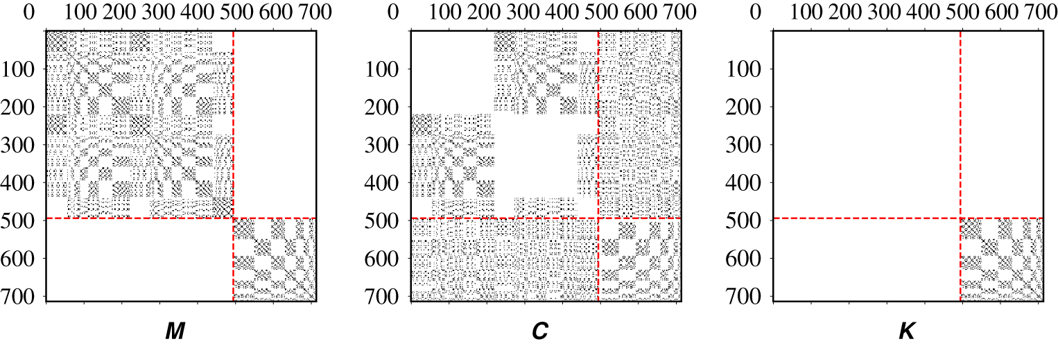
Schematic structure (non-zero entries) of the sparse matrices  $[\unicode[STIX]{x1D648},\unicode[STIX]{x1D63E},\unicode[STIX]{x1D646}]$ of QEP (4.1) with
 $M_{S}=0$,
 $M_{A}=0$ and
 $\mathbf{1}_{\unicode[STIX]{x1D6FA}}=\mathbf{1}_{z}$. Polynomial degree
 $n=10$ with the dimensions of the finite-dimensional spaces
 $\dim \boldsymbol{{\mathcal{V}}}\,[0,10]=495$ and
 $\dim \boldsymbol{{\mathcal{W}}}\,[0,10]=219$. Dashed (red) lines illustrate the block structures associated with the coupling between the trial and test subspaces. Upper left block: test and trial elements in
 $\boldsymbol{V}\,[0,10]$. Upper right block: test elements in
 $\boldsymbol{{\mathcal{V}}}\,[0,10]$ and trial elements in
 $\boldsymbol{{\mathcal{W}}}\,[0,10]$. Lower left block: test elements in
 $\boldsymbol{{\mathcal{W}}}\,[0,10]$ and trial elements in
 $\boldsymbol{{\mathcal{V}}}\,[0,10]$. Lower right block: test and trial elements in
 $\boldsymbol{{\mathcal{W}}}\,[0,10]$.

In practice, we convert QEP (4.1) into a generalised eigenvalue problem (GEP) of size  $2N$. This process is called linearisation (Tisseur & Meerbergen Reference Tisseur and Meerbergen2001). To do so, we recast matrix quadratic problem (4.1) as
 $$\begin{eqnarray}\unicode[STIX]{x1D706}\left(\begin{array}{@{}cc@{}}\unicode[STIX]{x1D644} & 0\\ 0 & \unicode[STIX]{x1D648}\\ \end{array}\right)\left(\begin{array}{@{}c@{}}\unicode[STIX]{x1D736}\\ \unicode[STIX]{x1D706}\unicode[STIX]{x1D736}\\ \end{array}\right)=\left(\begin{array}{@{}cc@{}}0 & \unicode[STIX]{x1D644}\\ -\unicode[STIX]{x1D646} & -\unicode[STIX]{x1D63E}\\ \end{array}\right)\left(\begin{array}{@{}c@{}}\unicode[STIX]{x1D736}\\ \unicode[STIX]{x1D706}\unicode[STIX]{x1D736}\\ \end{array}\right),\end{eqnarray}$$
where  $\unicode[STIX]{x1D644}$ is the identity matrix. An obvious difference with QEP (4.1) is that GEP (4.3) has
 $2N$ eigenvalues (possibly degenerate), although we have only
 $N$ unknowns in the problem. However, because
 $[\unicode[STIX]{x1D648},\unicode[STIX]{x1D63E},\unicode[STIX]{x1D646}]$ are real-valued matrices, the eigenvalues come in eigen-pairs
 $[\unicode[STIX]{x1D706},\unicode[STIX]{x1D736}]$ and
 $[\unicode[STIX]{x1D706}^{\dagger },\unicode[STIX]{x1D736}^{\dagger }]$ (Tisseur & Meerbergen Reference Tisseur and Meerbergen2001). Hence, the effective number of eigenvalues and eigenvectors reduces to
 $N$. The typical matrix structure for a rotating and non-magnetic configuration is shown in figure 3. The matrices are (relatively) sparse and with block structures. For instance, the matrix
 $\unicode[STIX]{x1D648}$ has a structure directly stemming from the orthogonality condition of the Helmholtz–Hodge decomposition. The matrix is not diagonal, since we do not orthogonalise the basis elements. Additionally, we observe that only the compressible space
 $\boldsymbol{{\mathcal{W}}}\,[0,n]$ yields non-zero entries in the matrix
 $\unicode[STIX]{x1D646}$ (when
 $M_{A}=0$), as delimited by the dashed lines in figure 3. Although the matrices are sparse, we have used a built-in direct solver for dense matrices based on the generalised Schur decomposition (since we are interested in the full spectrum).
4.2 Incompressible modes $\boldsymbol{{\mathcal{V}}}\,[0,n]$

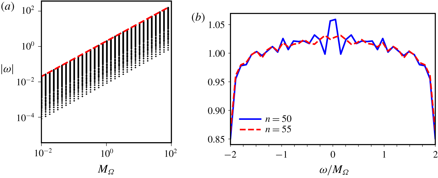
Inertial modes described by the finite-dimensional space  $\boldsymbol{{\mathcal{V}}}\,[0,n]$. (a) Spectrum, as a function of
 $M_{\unicode[STIX]{x1D6FA}}$, in rotating spheres at the polynomial degree
 $n=15$. The angular frequency scales linearly with the rotational Mach number with
 $|\unicode[STIX]{x1D714}|/M_{\unicode[STIX]{x1D6FA}}<2$. Dashed (red) line shows the upper bound
 $2\,M_{\unicode[STIX]{x1D6FA}}$, which is not an allowed eigenvalue (e.g. Backus & Rieutord Reference Backus and Rieutord2017). (b) Relative frequency histogram in spheres for
 $n=50$ (45 475 modes) and
 $n=55$ (60 060 modes). The number of classes (of uniform length) is 40.

By considering the solenoidal space  $\boldsymbol{{\mathcal{V}}}\,[0,n]$ alone, the compressible term vanishes in (2.11) to yield incompressible modes. Among them, the inertial modes play a fundamental role in rotating flows (e.g. Le Bars et al. Reference Le Bars, Cébron and Le Gal2015; Zhang & Liao Reference Zhang and Liao2017). The inertial modes of a given spatial complexity are exactly described by the finite-dimensional space
 $\boldsymbol{{\mathcal{V}}}\,[0,n]$ (Vantieghem Reference Vantieghem2014). Moreover, Backus & Rieutord (Reference Backus and Rieutord2017) and Ivers (Reference Ivers2017) proved mathematically that any solenoidal flow in rigid ellipsoids can be expanded onto a linear combination of inertial modes. This rigorously ensures the completeness of the polynomial space
 $\boldsymbol{{\mathcal{V}}}\,[0,n]$ in the limit
 $n\rightarrow \infty$ (for square-integrable vector fields).
The spectrum of the inertial modes is illustrated in figure 4. The eigenvalue is purely imaginary  $\unicode[STIX]{x1D706}=\text{i}\unicode[STIX]{x1D714}$, with an angular frequency
 $\unicode[STIX]{x1D714}$ which is bounded by
 $|\unicode[STIX]{x1D714}|/M_{\unicode[STIX]{x1D6FA}}<2$ (e.g. Greenspan Reference Greenspan1968). In compressible units, the frequency grows linearly with
 $M_{\unicode[STIX]{x1D6FA}}$ as shown in figure 4(a). Yet, the probability density function of the inertial modes, within the interval
 $|\unicode[STIX]{x1D714}|/M_{\unicode[STIX]{x1D6FA}}<2$, has not been reported yet. We show in figure 4(b) the (sampled) probability density function, obtained by increasing the polynomial degree for values as large as
 $n\leqslant 55$. This suggests that the probability density function of the inertial modes is nearly uniform in spheres. This behaviour starts emerging when considering large enough polynomial degrees (
 $n\geqslant 55$).
Finally, various modes exist in the presence of magnetic fields. The hydrodynamic modes have been already discussed in spheres (e.g. Malkus Reference Malkus1967; Friedlander Reference Friedlander1987; Zhang, Liao & Schubert Reference Zhang, Liao and Schubert2003; Labbé et al. Reference Labbé, Jault and Gillet2015) and do survive in ellipsoids (Vidal et al. Reference Vidal, Cébron, ud Doula and Alecian2019).
4.3 Compressible modes $\boldsymbol{{\mathcal{W}}}\,[0,n]$

We seek compressible solutions  $\unicode[STIX]{x1D743}=\unicode[STIX]{x1D735}\unicode[STIX]{x1D6F7}_{w}\in \boldsymbol{{\mathcal{W}}}$, by considering non-rotating and non-magnetic configurations. Then, QEP (4.1) simply reduces to the Helmholtz equation with a Neumann boundary condition, that is
 $$\begin{eqnarray}\unicode[STIX]{x1D706}^{2}\unicode[STIX]{x1D6F7}_{w}=\unicode[STIX]{x1D6FB}^{2}\unicode[STIX]{x1D6F7}_{w},\quad \unicode[STIX]{x1D735}\unicode[STIX]{x1D6F7}_{w}\boldsymbol{\cdot }\mathbf{1}_{n}=0\quad \text{on}~\unicode[STIX]{x2202}V,\end{eqnarray}$$
with  $\unicode[STIX]{x1D706}=\text{i}\unicode[STIX]{x1D714}$ the eigenvalue and
 $\unicode[STIX]{x1D714}\in \mathbb{R}$ the angular frequency. The decay rate is rigorously zero for the non-penetration condition in the absence of diffusive effects (Willatzen & Lew Yan Voon Reference Willatzen and Lew Yan Voon2004). We could seek polynomial solutions of (4.4) belonging to
 $\boldsymbol{{\mathcal{W}}}\,[0,n]$, by directly applying the method of weighted residuals (see Vidal et al. (Reference Vidal, Su and Cébron2019b), but with a Dirichlet boundary condition on
 $\unicode[STIX]{x1D6F7}_{w}$). However, this approach is less general than solving (4.1), because it cannot be consistently extended to account for rotation (see appendix C). Nonetheless, discussing the solutions of (4.4) is worthy of interest to validate the polynomial solutions against known analytical solutions.
Analytical solutions of (4.4) can be obtained in spheroids (Chang Reference Chang1971, Reference Chang1972) and ellipsoids (Willatzen & Lew Yan Voon Reference Willatzen and Lew Yan Voon2004), by using separation of variables in ellipsoidal coordinates. To benchmark the polynomial description, we consider axisymmetric spheroids ( $a=b\neq c$) for which the eigenfrequencies have been tabulated (only for a few configurations in Chang (Reference Chang1971, Reference Chang1972)). They are characterised by a triplet
 $(i,l,m)$ with
 $i$ an index characterising the radial-like complexity,
 $l$ the meridional wavenumber (e.g. the spherical harmonic degree in spheres) and
 $m\in \mathbb{Z}$ the azimuthal wavenumber (with an azimuthal Fourier decomposition in
 $\exp (\text{i}m\unicode[STIX]{x1D719})$). Because of the symmetry of revolution, the modes characterised by the same doublet
 $(i,l)$ but with different
 $m$ are degenerate, that is, have the same angular frequency. For a given doublet
 $(l,m)$, we denote
 $\unicode[STIX]{x1D714}_{i,l,m}$ the angular frequency of the
 $i$th spheroidal acoustic mode. This frequency is given by the
 $i$th zero of the first derivative (with respect to the radial-like variable) of the prolate (
 $c\geqslant a$) or oblate (
 $a\geqslant c$) spheroidal function of the first kind for a Neumann condition on
 $\unicode[STIX]{x1D6F7}_{w}$. The solutions
 $i=1$ are the fundamental modes, the ones with
 $i=2$ the first harmonics and so on. Contrary to the inertial modes in figure 4, the acoustic modes have a spectrum with a non-uniform (discrete) distribution.
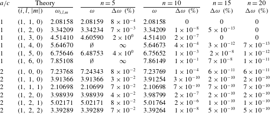
Angular frequency  $\unicode[STIX]{x1D714}$ of acoustic modes in spheroids (
 $a=b$). Comparison between analytical predictions
 $\unicode[STIX]{x1D714}_{i,l,m}$ (from Chang Reference Chang1972) and polynomial solutions belonging to
 $\boldsymbol{{\mathcal{W}}}\,[0,n]$ (up to the truncation degree
 $n=20$). The relative error
 $\unicode[STIX]{x0394}\unicode[STIX]{x1D714}$ is given by expression (4.5). The symbol
 $\emptyset$ means that the modes do not appear in the spectrum for this polynomial degree.

We show in table 2 the comparison between theoretical predictions and polynomial solutions, for a few fundamental modes in spheroids. All the eigenvalues are imaginary, that is  $\unicode[STIX]{x1D706}=\text{i}\unicode[STIX]{x1D714}$ with
 $\unicode[STIX]{x1D714}\in \mathbb{R}$. The real part is numerically zero (up to the machine precision, not shown). Then, we vary the truncation degree
 $n$ to outline how the numerical convergence is affected. We cannot expect the polynomial decomposition to be as efficient as a separable spectral decomposition (for instance using spherical harmonics), which diagonalises exactly Helmholtz equation (4.4). We compute the relative error (between numerics and theory) on the angular frequency
 $$\begin{eqnarray}\unicode[STIX]{x0394}\unicode[STIX]{x1D714}=|\unicode[STIX]{x1D714}-\unicode[STIX]{x1D714}_{i,l,m}|/\unicode[STIX]{x1D714}_{i,l,m},\end{eqnarray}$$
as a function of the truncation degree  $n$. Expression (4.5) gives a good proxy of the convergence for eigenvalue computations (e.g. Valdettaro et al. Reference Valdettaro, Rieutord, Braconnier and Frayssé2007). We find that only the first modes are approximatively described by the polynomial expansion at small degrees (e.g. at
 $n=5$ in spheres), with a relative error smaller than 10 %. Modes with higher spatial complexity are not captured at this polynomial degree, for instance the spherical mode (1, 6, 0). Increasing
 $n$ is required for the modes to appear in the spectrum (here at
 $n=10$). When
 $n$ is further increased, we observe that the relative errors become extremely small for this subset of modes. The azimuthal degeneracy of the modes is also well recovered, up to the machine precision (when
 $n$ is large enough, not shown).
Even if the polynomial description is not exact, polynomial solutions of (4.4) are accurate when  $n$ is large enough. Its accuracy is rooted in the Taylor expansion of the (known) analytical solutions. In spheres (
 $a=c$), spheroidal modes reduce to the textbook solutions in spherical coordinates
 $(r,\unicode[STIX]{x1D703},\unicode[STIX]{x1D719})$
 $$\begin{eqnarray}\unicode[STIX]{x1D6F7}_{w}(r,\unicode[STIX]{x1D703},\unicode[STIX]{x1D719})\propto j_{l}(r\unicode[STIX]{x1D714}_{i,l,m})\,{\mathcal{Y}}_{l}^{m}(\unicode[STIX]{x1D703},\unicode[STIX]{x1D719}),\end{eqnarray}$$
with  ${\mathcal{Y}}_{l}^{m}(\unicode[STIX]{x1D703},\unicode[STIX]{x1D719})$ the spherical harmonic (of degree
 $l$ and azimuthal order
 $m$) and the associated spherical Bessel function
 $j_{l}(r\unicode[STIX]{x1D714}_{i,l,m})$. The latter admits a convergent series in powers of
 $r^{2}=x^{2}+y^{2}+z^{2}$ (e.g. § 10 in Abramovitz & Stegun (Reference Abramovitz and Stegun1971)). Solution (4.6) has then the infinite polynomial expansion
 $\unicode[STIX]{x1D6F7}_{w}\propto r^{l}{\mathcal{Y}}_{l}^{m}\,T(r^{2})$, where
 $r^{l}{\mathcal{Y}}_{l}^{m}$ is a homogeneous Cartesian polynomial of degree
 $l$ (i.e. a solid spherical harmonic) and
 $T(r^{2})$ a power series. Thus, the (almost) arbitrary accuracy of the polynomial description is equivalent to vary the truncation in the power series
 $T(r^{2})$. Similar expansions could be obtained in ellipsoids (albeit often not explicitly), due to the Cartesian form of the ellipsoidal harmonics (e.g. Dassios Reference Dassios2012).
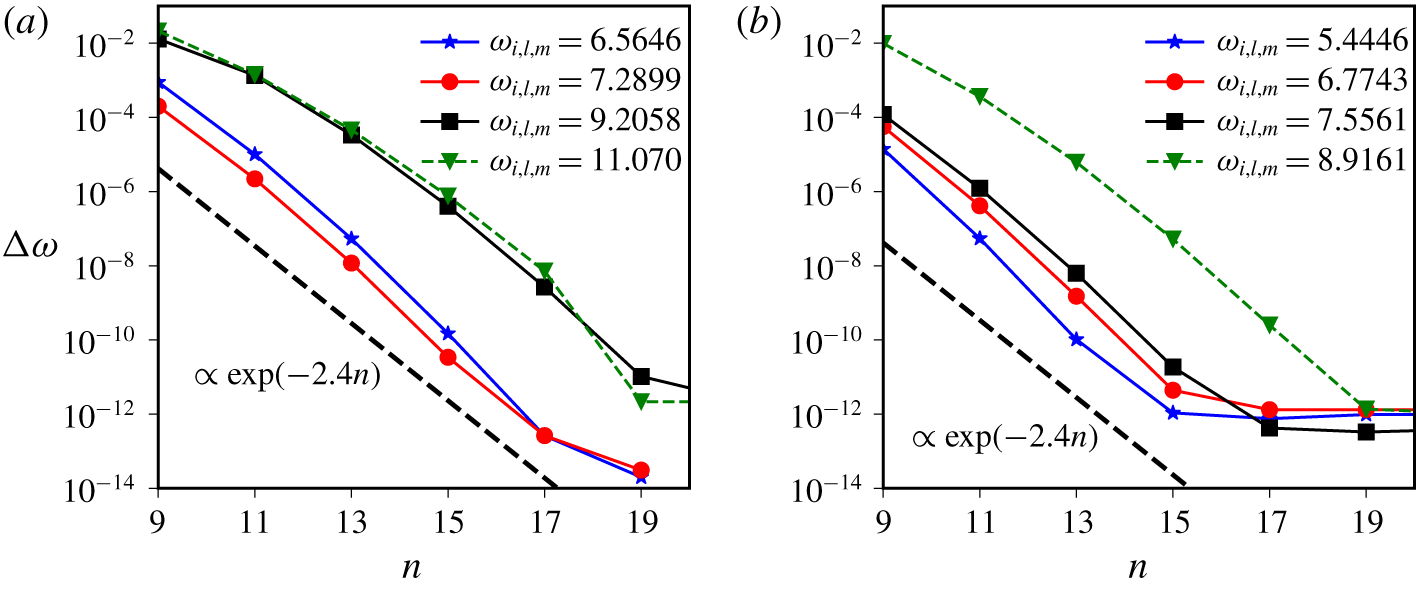
Spectral convergence of the polynomial solutions in  $\boldsymbol{{\mathcal{W}}}\,[0,n]$, as a function of the truncation degree
 $n$. Relative error
 $\unicode[STIX]{x0394}\unicode[STIX]{x1D714}$ between numerics
 $\unicode[STIX]{x1D714}$ and high-precision predictions
 $\unicode[STIX]{x1D714}_{i,l,m}$ in (a) spheres (
 $a=b=c=1$) and (b) an oblate spheroid (
 $a=b=1,c=0.5$). Black dashed lines show the spectral convergence
 $\unicode[STIX]{x0394}\unicode[STIX]{x1D714}\propto \exp (-2.4n)$. We have used for
 $\unicode[STIX]{x1D714}_{i,l,m}$ either high-precision analytical predictions (Chang Reference Chang1972) or high-resolution computations at
 $n=25$.

As outlined in table 2, the convergence towards the expected analytical eigenvalues is very fast for the modes with the largest spatial scales. We also quantify the convergence of the eigenvalues with the spatial resolution in figure 5. We show the evolution of relative error (4.5), as a function of the truncation degree  $n$. The polynomial description strikingly exhibits an exponential convergence, which is typical of accurate spectral methods (Boyd Reference Boyd2001). The errors decrease very fast, with the numerical scaling
 $\unicode[STIX]{x0394}\unicode[STIX]{x1D714}\propto \exp (-2.4n)$, until the computations are limited by the round-off errors of the eigenvalue solver (here around
 $10^{-12}{-}10^{-13}$). The errors then depart from an exponential decay, to become almost insensitive to the polynomial degree (as previously reported in table 2 for
 $n=20$). This plateau appears for large enough values of
 $n$ (depending on the spatial complexity of the modes). No better approximation to the eigenvalue can be obtained by increasing further the truncation degree
 $n$ with double-precision arithmetic. Yet, the numerical accuracy could be increased with computations using quadruple precision (as considered in Rieutord & Valdettaro (Reference Rieutord and Valdettaro2018)). Finally, the spectral polynomial method outperforms the (standard) finite-element computations performed with COMSOL in terms of numerical accuracy, as shown in appendix A. Indeed, the errors decrease much slower as a function of the spatial resolution, following only a power-law scaling that is characteristic of finite-element methods using piecewise continuous polynomials (Boyd Reference Boyd2001).
Therefore, we have shown that the (spectral) polynomial method is very efficient, due to its spectral convergence. In the following, we have considered truncation degrees  $n\leqslant 20$, which ensure an excellent convergence for all the modes we are interested in.
4.4 Rotational compressible modes
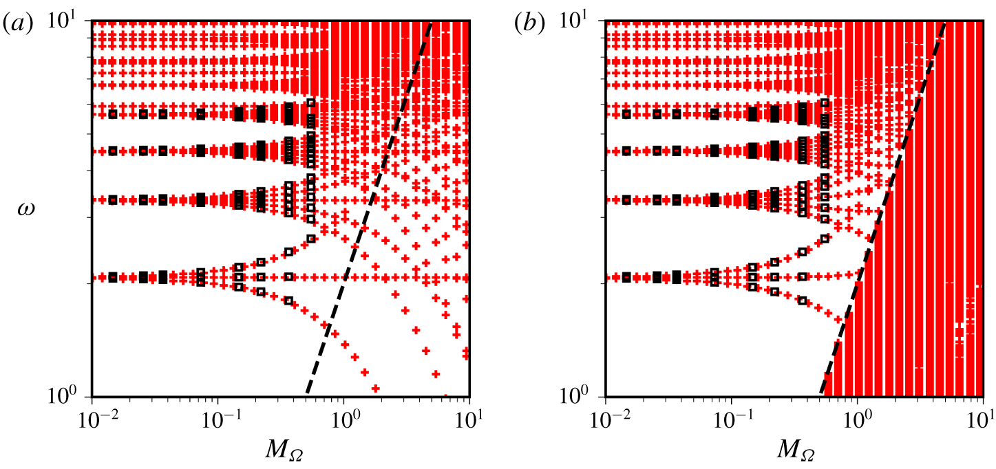
Rotating compressible modes in spheres ( $a=b=c=1$). Red crosses: polynomial solutions
 $\boldsymbol{{\mathcal{W}}}\,[0,20]$ in (a) and
 $\boldsymbol{{\mathcal{V}}}\,[0,20]\oplus \boldsymbol{{\mathcal{W}}}\,[0,20]$ in (b). Empty (black) squares: diffusive computations with COMSOL (separate
 $m$,
 $Re_{S}=4\times 10^{6}$,
 $\unicode[STIX]{x1D708}_{B}/\unicode[STIX]{x1D708}=0.6$), see details in appendix A. Dashed black lines show the upper bound
 $\unicode[STIX]{x1D714}=2\,M_{\unicode[STIX]{x1D6FA}}$ for inertial modes. The experimental range of parameters is
 $M_{\unicode[STIX]{x1D6FA}}\leqslant 2\times 10^{-1}$ (see table 1).

We reintroduce global rotation in the system, by assuming  $M_{\unicode[STIX]{x1D6FA}}\neq 0$ and
 $\mathbf{1}_{\unicode[STIX]{x1D6FA}}=\mathbf{1}_{z}$. When the system is rotating, the acoustic modes cannot be sought separately from the inertial modes in the polynomial space
 $\boldsymbol{{\mathcal{W}}}\,[0,n]$. Indeed, the incompressible and compressible spaces are now coupled through the Coriolis operator, as illustrated by the non-zero coupled entries of the matrix
 $\unicode[STIX]{x1D63E}$ in figure 3. Thus, we must seek a priori solutions in
 $\boldsymbol{{\mathcal{V}}}\,[0,n]\oplus \boldsymbol{{\mathcal{W}}}\,[0,n]$. Yet, in the relevant regime
 $M_{\unicode[STIX]{x1D6FA}}\ll 1$ (see table 1), we may still expect the acoustic modes to be essentially compressible (i.e. being mostly described by
 $\boldsymbol{{\mathcal{W}}}\,[0,n]$).
We first survey in figure 6 the whole spectrum in rotating spheres, computed by considering solely  $\boldsymbol{{\mathcal{W}}}\,[0,20]$ in (a) and
 $\boldsymbol{{\mathcal{V}}}\,[0,n]\oplus \boldsymbol{{\mathcal{W}}}\,[0,20]$ in (b). We have also superimposed targeted diffusive computations performed with COMSOL (see appendix A). They are in excellent agreement with the diffusionless polynomial solutions, thereby cross-validating the general results. Several points of figure 6 are worth commenting. We have not shown the range
 $M_{\unicode[STIX]{x1D6FA}}\geqslant 10$, where we get three families of modes. Two of them are in good agreement with a local analysis (not shown). The missing one results from the rotational splitting of the acoustic modes, which exists only in bounded geometries. Yet, the results for such large rotation rates are unlikely physical. Indeed, the centrifugal force has been entirely neglected in the analysis, although it may affect some acoustic modes for rapid rotation (Lignières et al. Reference Lignières, Rieutord and Reese2006; Reese et al. Reference Reese, Lignières and Rieutord2006). Moreover, the range
 $M_{\unicode[STIX]{x1D6FA}}\geqslant 1$ is unreachable in laboratory experiments (see table 1).
When  $M_{\unicode[STIX]{x1D6FA}}\leqslant 1$, the two spectra obviously differ by the presence of the inertial modes, associated with the space
 $\boldsymbol{{\mathcal{V}}}\,[0,20]$ in figure 6(b). Their frequency lies in the interval
 $|\unicode[STIX]{x1D714}|<2\,M_{\unicode[STIX]{x1D6FA}}$ (Valette Reference Valette1989a,Reference Valetteb), as for incompressible fluids (e.g. Backus & Rieutord Reference Backus and Rieutord2017). They are only weakly affected by compressibility when
 $M_{\unicode[STIX]{x1D6FA}}\leqslant 1$ (not shown). By contrast, the acoustic modes, located above the line
 $|\unicode[STIX]{x1D714}|\geqslant 2\,M_{\unicode[STIX]{x1D6FA}}$, are significantly affected by rotation. The latter lifts the azimuthal degeneracy of the spherical acoustic modes. More precisely, a non-rotating spherical solution
 $\unicode[STIX]{x1D714}_{i,l,m}$ splits into
 $2l+1$ distinct frequencies (Gough & Thompson Reference Gough and Thompson1990). For instance, the fundamental mode with
 $l=1$ splits into three branches (as observed), the second mode with
 $l=2$ into five branches and so on. This splitting is not predicted by a plane-wave analysis (not shown), such that Coriolis effects only occur in bounded geometries.
4.5 Magneto-acoustic modes
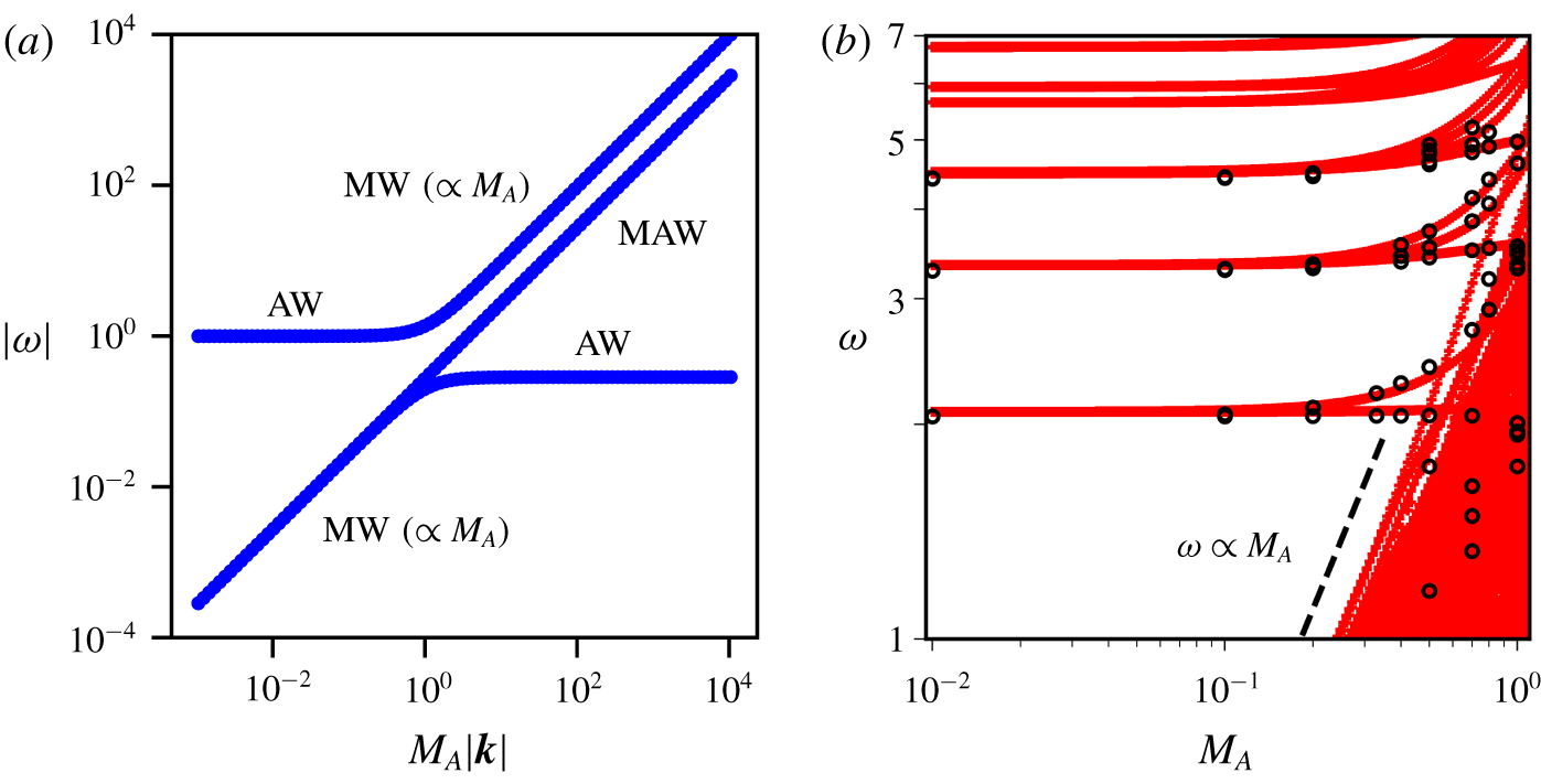
Angular frequency  $\unicode[STIX]{x1D714}$ of non-rotating magneto-acoustic modes as a function of
 $M_{A}$. (a) Plane-wave analysis for the wavenumber
 $\boldsymbol{k}=(0.1,1.0,0.3)^{\top }$. AW: acoustic waves. MW: magnetic (Alfvén) waves. MAW: magneto-acoustic waves. (b) Polynomial solutions in spheres for
 $\boldsymbol{{\mathcal{V}}}\,[0,15]\oplus \boldsymbol{{\mathcal{W}}}\,[0,15]$. Empty (black) circles: three-dimensional COMSOL diffusive solutions for
 $Re_{S}=10^{3}$ and
 $Rm_{S}=10$ (
 $\#\text{DOF}=416\,456$).

We finally consider non-rotating magnetic configurations ( $M_{A}\neq 0$). We investigate the regime
 $M_{A}\ll 1$, which is relevant for experiments (see table 1). Before solving numerically the bounded problem in rigid ellipsoids, it is worth pointing out the properties of the various waves with an unbounded (local) analysis. To do so, we assume that
 $\mathbf{1}_{B}=\mathbf{1}_{z}$ and
 $M_{\unicode[STIX]{x1D6FA}}=M_{S}=0$. Then, we seek plane-wave solutions
 $\unicode[STIX]{x1D743}\propto \exp (\text{i}\boldsymbol{k}\boldsymbol{\cdot }\boldsymbol{r})$, with
 $\boldsymbol{k}$ the (local) wave vector. The typical plane-wave spectrum is shown in figure 7(a). We observe a change of regime, depending on the strength of the background magnetic field (measured by
 $M_{A}$). The transition occurs around
 $M_{A}|\boldsymbol{k}|\simeq 1$. In the strong field regime (
 $M_{A}|\boldsymbol{k}|\geqslant 1$), we get three branches of magneto-acoustic waves. The fast branch is made of magnetic (Alfvén) waves, with a dimensionless angular frequency
 $|\unicode[STIX]{x1D714}|\propto M_{A}$. The slow waves are almost pure acoustic waves, constrained to move along magnetic field lines (e.g. Campos Reference Campos1987). The intermediate branch represents hybrid magneto-acoustic waves. In the weak field regime (
 $M_{A}|\boldsymbol{k}|\leqslant 1$), these three branches coalesce to yield two branches. The acoustic waves become the fast waves and the Alfvén waves the slow ones.
We illustrate in figure 7(b) the modal spectrum in non-rotating magnetised spheres, as a function of  $M_{A}$. We have also compared our diffusionless polynomial modes with three-dimensional (3-D) diffusive computations obtained with COMSOL. Computing magnetic solutions with COMSOL is numerically challenging in three dimensions. Thus, because of numerical constraints, we have fixed the diffusive numbers
 $Re_{S}=10^{3}$ and
 $Rm_{S}=10$. We have used 416 456 degrees of freedom for these computations. This yields a resolution of approximately 50 points in each spatial direction. We refer the reader to appendix A for additional details on the numerics. We find a broad agreement between the polynomial solutions and the 3-D diffusive solutions (for both the Alfvén modes and the acoustic modes, see below). The discrepancies, usually smaller than 10-1, are due to the large diffusive effects (absent in our diffusionless polynomial method) and to the lack of spectral decomposition in the azimuthal direction (in the 3-D finite-element computations). We have checked that we slowly approach the diffusionless solutions by increasing
 $Re_{S}$ and
 $Rm_{S}$ (not shown). Then, several points are worth commenting in figure 7(b). We obtain two families of modes. On the one hand, the slow family (when
 $M_{A}\leqslant 1$) disappears by considering only the compressible space
 $\boldsymbol{{\mathcal{W}}}\,[0,n]$ (not shown), and their angular frequency scales as
 $\unicode[STIX]{x1D714}\propto M_{A}$. This clearly shows that these modes are the magnetic Alfvén modes, mainly associated with the incompressible space
 $\boldsymbol{{\mathcal{V}}}\,[0,n]$. Their eigenfrequencies scale as in the local theory (e.g. Campos Reference Campos1987). On the other hand, the fast modes do survive when we suppress the divergenceless space (not shown). They are acoustic modes, only slightly perturbed by the magnetic field (when
 $M_{A}\leqslant 1$). Moreover, the magnetic field lifts the azimuthal degeneracy of the acoustic part of the spectrum. This was also found by Gough & Thompson (Reference Gough and Thompson1990) with perturbation theory, but they considered different background magnetic fields.
Therefore, we have recovered the two families of magneto-acoustic modes in this regime, as predicted by the local theory. We do not study further the modes in rotating magnetised spheres. Indeed, the properties of the incompressible modes should remain largely valid for their compressible counterparts. The Alfvén modes have also been observed and discussed in the experimental context (e.g. in rotating fluids, see Schmitt et al. (Reference Schmitt, Alboussiere, Brito, Cardin, Gagnière, Jault and Nataf2008) and Tigrine et al. (Reference Tigrine, Nataf, Schaeffer, Cardin and Plunian2019)). Moreover, we will show that magnetic effects are negligible on the acoustic spectrum, such that the interplay between rotation and magnetic field is not worth investigating for MAV.
5 Acoustic splittings for MAV
We revisit the properties of the acoustic modes in relation to MAV for experiments. The small values of  $M_{A}$ in experiments (see table 1) suggest that magnetic fields would have very tiny influence in experiments. We confirm this assumption in appendix B, such that we discard magnetic effects in the following. We investigate quantitatively how the ellipsoidal flattening and rotation along
 $\mathbf{1}_{\unicode[STIX]{x1D6FA}}=\mathbf{1}_{z}$ alter the (initially degenerate) spherical acoustic modes. Dimensionless variations as small as
 $10^{-4}{-}10^{-3}$ can be measured in air experiments (Su et al. Reference Su, Cébron, Nataf, Cardin, Vidal, Solazzo and Do2020) and, thus, should be accurately computed. Similarly, we leave aside the effects of a background flow by setting
 $M_{S}=0$. The general method is only presented in appendix B. Quantitative results with
 $M_{S}\neq 0$ are problem dependent and beyond the scope of the present study. Applications for flow inversions will be provided elsewhere, related to the ZoRo experiment (Su et al. Reference Su, Cébron, Nataf, Cardin, Vidal, Solazzo and Do2020).
The full ellipsoid is a canonical situation, in which perturbation theory can be carefully assessed against non-perturbative solutions (due to the existence of the polynomial solutions). To quantify ellipticity effects, we introduce the polar flattening
 $$\begin{eqnarray}\unicode[STIX]{x1D716}=(a-c)/a.\end{eqnarray}$$
Oblate containers are characterised by  $0\leqslant \unicode[STIX]{x1D716}\leqslant 1$ and prolate ones by
 $-1\leqslant \unicode[STIX]{x1D716}\leqslant 0$. We mainly focus on spheroidal geometries (i.e.
 $a=b$), to have a single deformation parameter
 $\unicode[STIX]{x1D716}$. Typical experimental values are
 $\unicode[STIX]{x1D716}=0.05$ in the ZoRo gas experiment (Su et al. Reference Su, Cébron, Nataf, Cardin, Vidal, Solazzo and Do2020),
 $\unicode[STIX]{x1D716}=0.04$ in precessing water experiments (e.g. Noir et al. Reference Noir, Brito, Aldridge and Cardin2001),
 $\unicode[STIX]{x1D716}\leqslant 0.3$ in librating water experiments (e.g. Lemasquerier et al. Reference Lemasquerier, Grannan, Vidal, Cébron, Favier, Le Bars and Aurnou2017; Le Reun et al. Reference Le Reun, Favier and Le Bars2019) or
 $\unicode[STIX]{x1D716}=0.08$ in tidal experiments (e.g. Grannan et al. Reference Grannan, Favier, Le Bars and Aurnou2016). So far, only small departures from spherical solutions have been considered and validated (Mehl Reference Mehl2007; Su et al. Reference Su, Cébron, Nataf, Cardin, Vidal, Solazzo and Do2020). Yet, since the polar flattening can have quite large values, significant effects could have been discarded. Note that the domain of validity of perturbation computations has been assessed in astrophysics up to
 $\unicode[STIX]{x1D716}\leqslant 0.16$ (Lignières et al. Reference Lignières, Rieutord and Reese2006; Reese et al. Reference Reese, Lignières and Rieutord2006), by increasing global rotation (which is responsible for spheroidal shapes due to centrifugal effects with a free-surface condition). Yet, these works cannot be used to disentangle easily the effects due to the ellipticity and rotation in rigid ellipsoids. Indeed, the rotation rate and the flattening are two independent parameters in experimental conditions. Hence, their effects remain to be carefully evaluated for MAV.
We denote in the following  $\unicode[STIX]{x1D714}(\unicode[STIX]{x1D716},M_{\unicode[STIX]{x1D6FA}})$ the angular eigenfrequency of the consistent solutions (without approximation) and
 $\unicode[STIX]{x1D714}(0,0)$ the ones of the acoustics modes in non-rotating spheres (
 $\unicode[STIX]{x1D716}=0,M_{\unicode[STIX]{x1D6FA}}=0$). Then,
 $\unicode[STIX]{x1D714}(0,0)$ is shifted by small amounts due to flattening
 $\unicode[STIX]{x1D6FF}_{\unicode[STIX]{x1D716}}$ and rotation
 $\unicode[STIX]{x1D6FF}_{\unicode[STIX]{x1D6FA}}$ along
 $\mathbf{1}_{\unicode[STIX]{x1D6FA}}=\mathbf{1}_{z}$. In the perturbation framework, these effects are often treated separately. If this assumption were consistent for experimental conditions, we would obtain
 $$\begin{eqnarray}\unicode[STIX]{x1D714}(\unicode[STIX]{x1D716},M_{\unicode[STIX]{x1D6FA}})\simeq \unicode[STIX]{x1D714}(0,0)+\unicode[STIX]{x1D6FF}_{\unicode[STIX]{x1D716}}+\unicode[STIX]{x1D6FF}_{\unicode[STIX]{x1D6FA}}.\end{eqnarray}$$
The residual of expression (5.2), denoted  $\unicode[STIX]{x1D6FF}_{\unicode[STIX]{x1D716}\unicode[STIX]{x1D6FA}}$, is due to any cross-effect between ellipticity and rotation. The frequency shifts would be given by
 $$\begin{eqnarray}\unicode[STIX]{x1D6FF}_{\unicode[STIX]{x1D716}}=\unicode[STIX]{x1D714}(\unicode[STIX]{x1D716},0)-\unicode[STIX]{x1D714}(0,0),\quad \unicode[STIX]{x1D6FF}_{\unicode[STIX]{x1D6FA}}=\unicode[STIX]{x1D714}(0,M_{\unicode[STIX]{x1D6FA}})-\unicode[STIX]{x1D714}(0,0).\end{eqnarray}$$
We assess separately ellipticity effects  $\unicode[STIX]{x1D6FF}_{\unicode[STIX]{x1D716}}$ in § 5.1 and rotational ones
 $\unicode[STIX]{x1D6FF}_{\unicode[STIX]{x1D6FA}}$ in § 5.2. They are then combined in § 5.3 to assess approximation (5.2), which neglects any possible cross-effect
 $\unicode[STIX]{x1D6FF}_{\unicode[STIX]{x1D716}\unicode[STIX]{x1D6FA}}$ between rotation and flattening.
5.1 Flattening effects
Ellipsoidal splitting of the first low-frequency acoustic modes in spheroids and triaxial ellipsoids. Polynomial solutions belonging to  $\boldsymbol{{\mathcal{W}}}\,[0,20]$. Ellipsoidal geometries
 $a=b=1,\,c=1-\unicode[STIX]{x1D716}$ in (a) and
 $a=1,\,b=1+\unicode[STIX]{x1D716},\,c=1-\unicode[STIX]{x1D716}$ in (b). Blue triangles: diffusionless COMSOL computations (using the built-in acoustic scalar equation).

We investigate quantitatively the ellipticity splitting of the compressible modes belonging to  $\boldsymbol{{\mathcal{W}}}\,[0,n]$, to assess the validity of perturbation theory in ellipsoids. Ellipticity effects are usually modelled with first-order perturbation theory (see in metrology Guianvarch et al. (Reference Guianvarch, Pitre, Bruneau and Bruneau2009)), but Mehl (Reference Mehl2007) extended the theory up to the second order. However, moderate ellipsoidal deformations are often encountered in fluid experiments, for which the perturbation approximation may be inaccurate. The various modes given in table 2 for spheroidal axisymmetric geometries have illustrated that an ellipsoidal boundary lifts the azimuthal degeneracy in
 $|m|$ of the spherical modes, for a given doublet
 $(i,l)$. Indeed, the degeneracy of the modes
 $(1,2,|m|)$, with
 $|m|\in [1,2,3]$, is lifted as the spherical cavity is squashed. Yet, the degeneracy of positive and negative
 $m$ is not removed in spheroids (not shown).
We show in figure 8(a) how ellipticity affects several low-frequency acoustic modes, as a function of the polar flattening  $\unicode[STIX]{x1D716}$ in spheroids. We clearly observe that the degeneracy of the spherical modes (
 $\unicode[STIX]{x1D716}=0$) is lifted by ellipsoidal flattening. Yet, the different branches, each associated with a given azimuthal number
 $m$ in the spheroidal geometry, are not modified in the same way. A naive first-order theory would predict that the frequency shift is linear in
 $\unicode[STIX]{x1D716}$. This is obviously not the case for some modes at moderate deformations
 $|\unicode[STIX]{x1D716}|\geqslant 0.2$. Some curves are closer to parabolas than to straight lines, such that they could be fairly described by second-order perturbation theory (Mehl Reference Mehl2007). In the strong deformation limit, the acoustic branches tend to diverge and crossings can occur between branches associated with different azimuthal modes in the initial spherical geometry (e.g. near
 $\unicode[STIX]{x1D714}=4.5$ at
 $\unicode[STIX]{x1D716}\simeq 0.4$ in figure 8a). Finally, we illustrate some triaxial configurations in figure 8(b) (for the first low-frequency modes), by assuming
 $b=a(1+\unicode[STIX]{x1D716})$ and
 $c=a(1-\unicode[STIX]{x1D716})$ with
 $a=1$ (in dimensionless units). The curves are symmetric with respect to
 $\unicode[STIX]{x1D716}=0$, since the acoustic problem is invariant under an exchange of
 $b$ and
 $c$. As naively expected for these small deformations (
 $|\unicode[STIX]{x1D716}|\leqslant 0.05$), the branches are close to straight lines, in agreement with first-order theory for the ellipticity splitting.
Accidental degeneracy of acoustic modes due to flattening in spheroids ( $a=b=1\neq c$). Acoustic angular frequency
 $\unicode[STIX]{x1D714}$ as a function of the polar flattening
 $\unicode[STIX]{x1D716}$. Comparison between polynomial solutions in
 $\boldsymbol{{\mathcal{W}}}\,[0,20]$ (squares) and finite-element computations (solid lines) with COMSOL. Vertical dashed (magenta) line shows the polar flattening
 $\unicode[STIX]{x1D716}=0.05$ of the ZoRo experiment (Su et al. Reference Su, Cébron, Nataf, Cardin, Vidal, Solazzo and Do2020).

We have shown that ellipticity effects do not affect similarly all the acoustic branches in figure 8. The branches tend to diverge by increasing the flattening. Thus, accidental degeneracies of acoustic modes (with initially distinct frequencies in spheres) can occur for large deformations. Unexpectedly, accidental degeneracy also occurs for initially identical branches, due to high-order ellipticity effects. This striking feature is clearly illustrated in figure 9, for two low-frequency acoustic modes in spheroidal geometries. The  $m=1$ branches are straight lines, that is they are mainly affected by first-order ellipticity effects. However, the
 $m=0$ modes undergo second-order effects (i.e. in
 $\unicode[STIX]{x1D716}^{2}$), such that the
 $m=0$ branches cross the
 $m=1$ branches at small values of
 $\unicode[STIX]{x1D716}$. This is not an artefact of the polynomial description, since we also get this behaviour with the finite-element computations in COMSOL. The numerical agreement is excellent, because we can perform diffusionless computations without rotation in COMSOL (see appendix A). Thus, figure 9 completely cross-validates the diffusionless results, which are recovered by using the two methods. These points are not avoided crossings that may exist in spheroidal geometries (Lignières et al. Reference Lignières, Rieutord and Reese2006), since each branch has its own azimuthal symmetry. Moreover, it turns out that the crossing point in figure 9(a) occurs near
 $\unicode[STIX]{x1D716}\simeq 0.05$, that is the spheroidal deformation of the ZoRo experiment (Su et al. Reference Su, Cébron, Nataf, Cardin, Vidal, Solazzo and Do2020).
We illustrate in figure 10 the modes which are close to the accidental degeneracies observed in figure 9(a). We have represented the dimensionless acoustic pressure  $p_{1}\propto -\unicode[STIX]{x1D735}\boldsymbol{\cdot }\unicode[STIX]{x1D743}$. The two modes have large spatial scales, but different meridional structures and azimuthal numbers (
 $m=0$ and
 $m=1$). Note that these modes do not undergo avoided crossing. Indeed, they keep their own azimuthal (and longitudinal) structure from each side of the crossing point (not shown). Finally, we point out that large-scale modes are likely sensitive to the large-scale components of the background velocity field, which are (a priori) easier to determine with MAV. Thus, a poor identification of these two particular low-frequency modes in the experimental data would be certainly misleading for the acoustic inversion.
Meridional sections of the acoustic pressure  $p_{1}\propto -\unicode[STIX]{x1D735}\boldsymbol{\cdot }\unicode[STIX]{x1D743}$ of the modes near the accidental degeneracies observed in figure 9. Polynomial solutions in
 $\boldsymbol{{\mathcal{W}}}\,[0,20]$. Oblate spheroids (
 $a=b=1$) with
 $\unicode[STIX]{x1D716}=0.05$, as in the ZoRo experiment (Su et al. Reference Su, Cébron, Nataf, Cardin, Vidal, Solazzo and Do2020). Each section is taken in a meridional plane containing the
 $z$-axis, at the longitude
 $\unicode[STIX]{x1D719}$ measured from the long
 $x$-axis. Horizontal axis shows
 $\sqrt{x^{2}+y^{2}}$ at the longitude
 $\unicode[STIX]{x1D719}$. Colour bar shows
 $p_{1}$, with arbitrary amplitudes and phase shifts. Solid grey lines are positive iso-contours, whereas dashed grey lines represent negative iso-contours.

This unexpected phenomenon clearly shows that an accurate description of the acoustic modes is a prerequisite to any application of MAV (at least in moderately deformed ellipsoids). In particular, if one would like still to use domain perturbation theory in ellipsoids, we advocate to employ (at least) a second-order theory (Mehl Reference Mehl2007).
5.2 Rotational splitting
Rotational splitting of acoustic modes in spheres. Comparison between polynomial solutions belonging to  $\boldsymbol{{\mathcal{W}}}\,[0,20]$ (black squares) and
 $\boldsymbol{{\mathcal{V}}}\,[0,20]\oplus \boldsymbol{{\mathcal{W}}}\,[0,20]$ (red lines). Blue triangles: COMSOL diffusive computations (separate
 $m$,
 $Re_{S}=4\times 10^{6}$,
 $\unicode[STIX]{x1D708}_{B}/\unicode[STIX]{x1D708}=0.6$). The experimental range of parameters is
 $M_{\unicode[STIX]{x1D6FA}}\leqslant 2\times 10^{-1}$ (see table 1).

We now focus on the frequency shift due to rotation  $\unicode[STIX]{x1D6FF}_{\unicode[STIX]{x1D6FA}}$ in the absence of deformation. Coming back to figure 6, we observe that the rotational shift seems to be accurately described solely by the compressible space
 $\boldsymbol{{\mathcal{W}}}\,[0,n]$ for small enough rotations. Indeed, the curves seem poorly distinguishable when
 $M_{\unicode[STIX]{x1D6FA}}\ll 10^{-1}$, whereas we do notice some differences when
 $M_{\unicode[STIX]{x1D6FA}}\geqslant 10^{-1}$ (for the intermediate branch of the first mode). This behaviour is confirmed in figure 11, in which we have superimposed the computations with
 $\boldsymbol{{\mathcal{W}}}\,[0,20]$ and
 $\boldsymbol{{\mathcal{V}}}\,[0,20]\oplus \boldsymbol{{\mathcal{W}}}\,[0,20]$. We illustrate only the two first modes, but we have checked that this behaviour remains valid for modes with higher frequencies (if their polynomial descriptions are well converged). The polynomial results are also in very good agreement with the 3-D computations in COMSOL (even if the latter necessarily include diffusion). This confirms the robustness of the results, even if the diffusive angular frequencies are slightly smaller (in absolute value) than the diffusionless frequencies. This is consistent with the diffusive theory (Moldover et al. Reference Moldover, Mehl and Greenspan1986). Thus, acoustic modes could be fairly described in the range
 $M_{\unicode[STIX]{x1D6FA}}\ll 10^{-1}$ by considering solely the space
 $\boldsymbol{{\mathcal{W}}}\,[0,n]$.
The frequency shift  $\unicode[STIX]{x1D6FF}_{\unicode[STIX]{x1D6FA}}$ is often estimated by first-order perturbation theory (e.g. Gough & Thompson Reference Gough and Thompson1990; Dahlen & Tromp Reference Dahlen and Tromp1998). Without centrifugal effects and when
 $M_{\unicode[STIX]{x1D6FA}}\ll 1$, we may expect the acoustic frequencies to scale linearly with rotation (i.e.
 $\unicode[STIX]{x1D6FF}_{\unicode[STIX]{x1D6FA}}\propto M_{\unicode[STIX]{x1D6FA}}$). Observing linear or quadratic effects (
 $\unicode[STIX]{x1D6FF}_{\unicode[STIX]{x1D6FA}}\propto M_{\unicode[STIX]{x1D6FA}}^{2}$) is not easy in figure 11, due to the log–linear representation. To disentangle the two scalings, we show in figure 12 the evolution of
 $|\unicode[STIX]{x1D6FF}_{\unicode[STIX]{x1D6FA}}|/M_{\unicode[STIX]{x1D6FA}}$, as a function of
 $M_{\unicode[STIX]{x1D6FA}}$ in the range
 $0\leqslant M_{\unicode[STIX]{x1D6FA}}\leqslant 10^{-1}$. For a dominant linear scaling,
 $|\unicode[STIX]{x1D6FF}_{\unicode[STIX]{x1D6FA}}|/M_{\unicode[STIX]{x1D6FA}}$ should be roughly constant. We have illustrated the observed behaviour for some low-frequency modes, which are representative of the results. We do obtain a linear variation
 $|\unicode[STIX]{x1D6FF}_{\unicode[STIX]{x1D6FA}}|\propto M_{\unicode[STIX]{x1D6FA}}$ when
 $M_{\unicode[STIX]{x1D6FA}}\leqslant 10^{-2}$, in agreement with first-order theory. When
 $M_{\unicode[STIX]{x1D6FA}}\leqslant 10^{-2}$, the typical error on the ratio
 $|\unicode[STIX]{x1D6FF}_{\unicode[STIX]{x1D6FA}}|/M_{\unicode[STIX]{x1D6FA}}$ is smaller than
 $10^{-3}$, yielding an upper-bound error on the frequency shift of
 $10^{-5}$. Then, second-order Coriolis effects are already present when
 $M_{\unicode[STIX]{x1D6FA}}\geqslant 10^{-2}$. At
 $M_{\unicode[STIX]{x1D6FA}}=10^{-1}$, the typical error is
 $3\times 10^{-2}$, yielding as typical estimate for the error on the frequency shift
 $3\times 10^{-3}$. Finally, we recover that the rotational shift is fairly described by considering space
 $\boldsymbol{{\mathcal{W}}}\,[0,n]$ when
 $M_{\unicode[STIX]{x1D6FA}}\ll 10^{-1}$. Moreover, high-order modes are less affected by the Coriolis force (not shown), as found experimentally (Su et al. Reference Su, Cébron, Nataf, Cardin, Vidal, Solazzo and Do2020) and in agreement with astrophysical predictions (Reese et al. Reference Reese, Lignières and Rieutord2006). We thus expect small Coriolis effects in the high-frequency regime.
Scaling of the rotational shift of acoustic modes in spheres ( $a=b=c=1$). Ratio
 $|\unicode[STIX]{x1D6FF}_{\unicode[STIX]{x1D6FA}}|/M_{\unicode[STIX]{x1D6FA}}$ as a function of
 $M_{\unicode[STIX]{x1D6FA}}$. Dashed black lines (respectively solid red lines) are polynomial solutions belonging to
 $\boldsymbol{{\mathcal{W}}}\,[0,20]$ (respectively
 $\boldsymbol{{\mathcal{V}}}\,[0,20]\oplus \boldsymbol{{\mathcal{W}}}\,[0,20]$).

Consequently, the linear approximation seems accurate enough for typical experimental purposes when  $M_{\unicode[STIX]{x1D6FA}}\leqslant 10^{-2}$. However, the linear approximation may not be sufficient for some large-scale modes and for large values of
 $M_{\unicode[STIX]{x1D6FA}}$, which can be considered in gas experiments (e.g. Su et al. Reference Su, Cébron, Nataf, Cardin, Vidal, Solazzo and Do2020).
5.3 Interplay between rotation and flattening
We have shown that, for typical experimental conditions (see table 1), ellipsoidal flattening is quickly responsible for second-order variations in  $\unicode[STIX]{x1D716}$, even for values as small as
 $\unicode[STIX]{x1D716}\leqslant 0.025$ (see figure 9). In addition, second-order Coriolis effects in
 $M_{\unicode[STIX]{x1D6FA}}$ might be also observed, notably in gas experiments (for which
 $M_{\unicode[STIX]{x1D6FA}}\leqslant 2\times 10^{-1}$). This leads us to naturally question the relevance of formal perturbation expansion (5.2), which treats independently ellipticity and rotational effects. Indeed, this approach rules out any possible cross-effect between rotation and flattening
 $\unicode[STIX]{x1D6FF}_{\unicode[STIX]{x1D716}\unicode[STIX]{x1D6FA}}$, which would scale as
 $\unicode[STIX]{x1D716}M_{\unicode[STIX]{x1D6FA}}$ at leading order. These effects may not be vanishingly small for experimental conditions, in which we can measure slight frequency changes of order
 $10^{-4}{-}10^{-3}$ (Su et al. Reference Su, Cébron, Nataf, Cardin, Vidal, Solazzo and Do2020).
Combined effects of rotation and ellipticity on acoustic modes in spheroids ( $a=b\neq c$). (a) Non-rotating acoustic branches, as a function of the polar flattening
 $\unicode[STIX]{x1D716}$. Solid (red) lines show the polynomial solutions in
 $\boldsymbol{{\mathcal{W}}}\,[0,20]$. Dashed (black) lines show the second-order perturbation theory, obtained with a quadratic fit of a few polynomial solutions when
 $\unicode[STIX]{x1D716}\ll 0.1$. (b) Angular frequency
 $\unicode[STIX]{x1D714}$ as a function of
 $M_{\unicode[STIX]{x1D6FA}}$. Red curves: non-perturbation solutions
 $\unicode[STIX]{x1D714}(\unicode[STIX]{x1D716},M_{\unicode[STIX]{x1D6FA}})$, computed from
 $\boldsymbol{{\mathcal{V}}}\,[0,20]\oplus \boldsymbol{{\mathcal{W}}}\,[0,20]$. Black squares: perturbation solutions (5.2), obtained by adding the frequency shift
 $\unicode[STIX]{x1D6FF}_{\unicode[STIX]{x1D716}}$ (due to ellipticity) and the rotating spherical solutions
 $\unicode[STIX]{x1D714}(0,M_{\unicode[STIX]{x1D6FA}})$. Frequency shift
 $\unicode[STIX]{x1D6FF}_{\unicode[STIX]{x1D716}}$ for each branch has been computed with formula (5.3), by using the non-rotating polynomial solutions shown in (a). Rotating spherical modes
 $\unicode[STIX]{x1D714}(0,M_{\unicode[STIX]{x1D6FA}})$ computed in
 $\boldsymbol{{\mathcal{V}}}\,[0,20]\oplus \boldsymbol{{\mathcal{W}}}\,[0,20]$.

Accurate estimates of  $\unicode[STIX]{x1D6FF}_{\unicode[STIX]{x1D716}}$ and
 $\unicode[STIX]{x1D6FF}_{\unicode[STIX]{x1D6FA}}$ are required to assess generic formula (5.2). We have shown that the polynomial method describes precisely
 $\unicode[STIX]{x1D6FF}_{\unicode[STIX]{x1D716}}$ and
 $\unicode[STIX]{x1D6FF}_{\unicode[STIX]{x1D6FA}}$ at any order. This is strongly different in perturbation theory. For instance,
 $\unicode[STIX]{x1D6FF}_{\unicode[STIX]{x1D716}}$ is usually limited to the second order in the deformation (Mehl Reference Mehl2007; Su et al. Reference Su, Cébron, Nataf, Cardin, Vidal, Solazzo and Do2020). However, second-order ellipticity effects are often not accurate enough (e.g. when
 $\unicode[STIX]{x1D716}=0.3$). We clearly illustrate this point in figure 13. We have first determined the rotating spherical solutions
 $\unicode[STIX]{x1D714}(0,M_{\unicode[STIX]{x1D6FA}})$ in
 $\boldsymbol{{\mathcal{V}}}\,[0,20]\oplus \boldsymbol{{\mathcal{W}}}\,[0,20]$. Second, we have computed the frequency shift
 $\unicode[STIX]{x1D6FF}_{\unicode[STIX]{x1D716}}$, in the absence of rotation, with formula (5.3). Each acoustic branch, characterised here by a given azimuthal number
 $m$, has its own frequency shift
 $\unicode[STIX]{x1D6FF}_{\unicode[STIX]{x1D716}}$. We have only considered the second-order ellipticity effects in
 $\unicode[STIX]{x1D6FF}_{\unicode[STIX]{x1D716}}$, which would be obtained with perturbation theory. To isolate these second-order effects, we have used a quadratic polynomial fit in powers of
 $\unicode[STIX]{x1D716}$ (dashed line in figure 13a), to describe the polynomial solutions (when
 $\unicode[STIX]{x1D716}\ll 0.1$). On the one hand, the fits are close to the true solutions when
 $\unicode[STIX]{x1D716}\leqslant 0.1$ (as naively expected). On the other hand, the fitted curves are far from the true branches for the upper acoustic branches when
 $\unicode[STIX]{x1D716}\geqslant 0.1$. It becomes obvious that second-order theory is largely inaccurate for the flattening
 $\unicode[STIX]{x1D716}=0.3$, even for the low-frequency modes. Computing
 $\unicode[STIX]{x1D6FF}_{\unicode[STIX]{x1D716}}$ from the quadratic law yields large errors in formula (5.2), as observed in figure 13(a). For the upper branches, the accurate estimates (containing all ellipticity effects) are
 $\unicode[STIX]{x1D6FF}_{\unicode[STIX]{x1D716}}(\unicode[STIX]{x1D716},0)=[0.4991,0.7121]$, whereas the fitted values are
 $\unicode[STIX]{x1D6FF}_{\unicode[STIX]{x1D716}}(\unicode[STIX]{x1D716},0)\simeq [0.5816,0.6518]$. These discrepancies would be directly responsible for erroneous predictions for the acoustic branches, as illustrated by the large offsets on the upper curves in figure 13(b).
Then, the goal is to evaluate the independence of ellipticity and Coriolis effects in expression (5.3). We assume that  $\unicode[STIX]{x1D6FF}_{\unicode[STIX]{x1D716}}$ contains all the effects due to ellipticity (without approximation) in the absence of rotation, whereas
 $\unicode[STIX]{x1D6FF}_{\unicode[STIX]{x1D6FA}}$ accounts for all the Coriolis effects (i.e. without the centrifugal effects, which have been entirely neglected) in the absence of ellipsoidal deformation. We assess formula (5.2) in figure 14, by considering two polar flattenings
 $\unicode[STIX]{x1D716}=0.05$ (e.g. Su et al. Reference Su, Cébron, Nataf, Cardin, Vidal, Solazzo and Do2020) and
 $\unicode[STIX]{x1D716}=0.3$ (e.g. Grannan et al. Reference Grannan, Favier, Le Bars and Aurnou2016; Lemasquerier et al. Reference Lemasquerier, Grannan, Vidal, Cébron, Favier, Le Bars and Aurnou2017). We have computed the frequency shift
 $\unicode[STIX]{x1D6FF}_{\unicode[STIX]{x1D716}}$ in the absence of rotation with formula (5.3). Each acoustic branch, characterised here by a given azimuthal number
 $m$, has its own frequency shift
 $\unicode[STIX]{x1D6FF}_{\unicode[STIX]{x1D716}}$. To avoid neglecting high-order ellipticity effects, the frequency shift
 $\unicode[STIX]{x1D6FF}_{\unicode[STIX]{x1D716}}$ is computed for each branch from accurate computations of
 $\unicode[STIX]{x1D714}(\unicode[STIX]{x1D716},0)$ and
 $\unicode[STIX]{x1D714}(0,0)$ in
 $\boldsymbol{{\mathcal{W}}}\,[0,20]$. We present illustrative results for some low-frequency modes.
Combined effects of rotation and flattening on acoustic modes in spheroids. Angular frequency  $\unicode[STIX]{x1D714}$ as a function of
 $M_{\unicode[STIX]{x1D6FA}}$. Red curves: non-perturbation solutions
 $\unicode[STIX]{x1D714}(\unicode[STIX]{x1D716},M_{\unicode[STIX]{x1D6FA}})$, computed in
 $\boldsymbol{{\mathcal{V}}}\,[0,20]\oplus \boldsymbol{{\mathcal{W}}}\,[0,20]$. Black squares: perturbation solutions (5.2), obtained by adding the frequency shift
 $\unicode[STIX]{x1D6FF}_{\unicode[STIX]{x1D716}}$ (due to ellipticity) to the rotating spherical solutions
 $\unicode[STIX]{x1D714}(0,M_{\unicode[STIX]{x1D6FA}})$. Frequency shift
 $\unicode[STIX]{x1D6FF}_{\unicode[STIX]{x1D716}}$ has been computed for each acoustic branch with formula (5.3), by using the non-rotating solutions in
 $\boldsymbol{{\mathcal{W}}}\,[0,20]$. Rotating spherical modes
 $\unicode[STIX]{x1D714}(0,M_{\unicode[STIX]{x1D6FA}})$ computed in
 $\boldsymbol{{\mathcal{V}}}\,[0,20]\oplus \boldsymbol{{\mathcal{W}}}\,[0,20]$. Blue triangles: COMSOL diffusive computations (separate
 $m$,
 $Re_{S}=4\times 10^{6}$,
 $\unicode[STIX]{x1D708}_{B}/\unicode[STIX]{x1D708}=0.6$). The experimental range of parameters is
 $M_{\unicode[STIX]{x1D6FA}}\leqslant 2\times 10^{-1}$ (see table 1).

We observe in figure 14(a) that perturbation solutions (5.2) seem in good agreement with the consistent solutions  $\unicode[STIX]{x1D714}(\unicode[STIX]{x1D716},M_{\unicode[STIX]{x1D6FA}})$ when
 $\unicode[STIX]{x1D716}=0.05$. However, this is largely a consequence of the chosen graphical representation. Quantitatively, we do obtain small discrepancies between the two approaches. They are due to cross-effects
 $\unicode[STIX]{x1D6FF}_{\unicode[STIX]{x1D716}M_{\unicode[STIX]{x1D6FA}}}$ in this figure, because the frequency shift
 $\unicode[STIX]{x1D6FF}_{\unicode[STIX]{x1D6FA}}$ contains any order of the Coriolis effects (independently of the ellipticity). Note that the error amplitude is also mode sensitive. Their typical magnitude is
 $\unicode[STIX]{x1D6FF}_{\unicode[STIX]{x1D716}M_{\unicode[STIX]{x1D6FA}}}\simeq c_{1}(M_{\unicode[STIX]{x1D6FA}})\,\unicode[STIX]{x1D716}M_{\unicode[STIX]{x1D6FA}}$, where the numerical prefactor is
 $c_{1}(M_{\unicode[STIX]{x1D6FA}})\leqslant 0.5$ when
 $M_{\unicode[STIX]{x1D6FA}}\leqslant 10^{-1}$. For instance, we get for the mode with
 $m=\pm 1$ at
 $M_{\unicode[STIX]{x1D6FA}}=10^{-1}$ in figure 14(a) a frequency shift around
 $1$ Hz (dimensional units), that is a dimensionless error of
 $4\times 10^{-3}$ on the angular frequency (not shown). Hence, we theoretically predict that cross-effects
 $\unicode[STIX]{x1D6FF}_{\unicode[STIX]{x1D716}\unicode[STIX]{x1D6FA}}$ are indeed observable in experiments. The situation is even much clearer for the ellipsoidal configuration
 $\unicode[STIX]{x1D716}=0.3$ illustrated in figure 14(b). For instance, the upper curves around
 $\unicode[STIX]{x1D714}=4.1$ differ in angular frequency by already 10-2 at
 $M_{\unicode[STIX]{x1D6FA}}=0.1$, which is one order of magnitude larger than for the lower branches. The frequency shift is then typically 10-3 when
 $M_{\unicode[STIX]{x1D6FA}}\simeq 10^{-2}$ for the upper branches and 10-4 for the lower ones in figure 14(b). Thus, we support that cross-effects between ellipticity and rotation are observable given the experimental precision (at least for some modes), even if they are discarded with perturbation theory (Su et al. Reference Su, Cébron, Nataf, Cardin, Vidal, Solazzo and Do2020).
5.4 Experimental implications
Combined effects of rotation and ellipticity on acoustic modes in spheroids ( $\unicode[STIX]{x1D716}=0.05$). (a) Angular frequency
 $\unicode[STIX]{x1D714}$ as a function of
 $M_{\unicode[STIX]{x1D6FA}}$. (b) Absolute splitting
 $\unicode[STIX]{x1D6FF}_{m}\unicode[STIX]{x1D714}$ between the acoustic branches of azimuthal wavenumbers
 $m$ and
 $-m$. Red curves: non-perturbation solutions
 $\unicode[STIX]{x1D714}(\unicode[STIX]{x1D716},M_{\unicode[STIX]{x1D6FA}})$, computed from
 $\boldsymbol{{\mathcal{V}}}\,[0,20]\oplus \boldsymbol{{\mathcal{W}}}\,[0,20]$. Dashed (black) curves: linear fit in
 $M_{\unicode[STIX]{x1D714}}$, modelling both first-order Coriolis effects
 $\unicode[STIX]{x1D6FF}_{\unicode[STIX]{x1D6FA}}$ and cross-effects
 $\unicode[STIX]{x1D6FF}_{\unicode[STIX]{x1D716}\unicode[STIX]{x1D6FA}}$ between ellipticity and rotation. The experimental range of parameters is
 $M_{\unicode[STIX]{x1D6FA}}\leqslant 2\times 10^{-1}$ (see table 1).

Previous results have direct implications for experiments. As shown in appendix B, magnetic splittings are far too small and can be safely ignored in the analysis. Yet, ellipticity and Coriolis effects can be significant and must be considered with care. For the ZoRo set-up ( $\unicode[STIX]{x1D716}=0.05$), Su et al. (Reference Su, Cébron, Nataf, Cardin, Vidal, Solazzo and Do2020) conducted a preliminary experimental survey with rotation, by using air at ambient temperature (
 $C_{0}^{\ast }\simeq 343~\text{m}~\text{s}^{-1}$). They confronted their experimental observations to a mixed perturbation theory similar to (5.2), taking into account second-order ellipticity effects and first-order Coriolis effects (without ellipticity). They considered (dimensional) rotation rate frequencies
 $\unicode[STIX]{x1D6FA}_{s}^{\ast }/(2\unicode[STIX]{x03C0})\leqslant 30$ Hz, that is
 $M_{\unicode[STIX]{x1D6FA}}\leqslant 10^{-1}$ in dimensionless units. The quantitative results outlined in figure 14(a) show that cross-effects are observable at
 $M_{\unicode[STIX]{x1D6FA}}=10^{-1}$. In particular, as also done in astrophysics (e.g. Aerts et al. Reference Aerts, Christensen-Dalsgaard and Kurtz2010), Su et al. (Reference Su, Cébron, Nataf, Cardin, Vidal, Solazzo and Do2020) measured the absolute acoustic splitting
 $\unicode[STIX]{x1D6FF}_{m}\unicode[STIX]{x1D714}$. The latter is the difference between the angular frequency of the acoustic branches with azimuthal wavenumbers
 $m$ and
 $-m$, that is
 $\unicode[STIX]{x1D6FF}_{m}\unicode[STIX]{x1D714}=|\unicode[STIX]{x1D714}(m)-\unicode[STIX]{x1D714}(-m)|$. Considering first-order perturbation theory for the Coriolis effects (without ellipticity), they observed small differences with their experimental data for the
 $|m|=1$ and
 $|m|=2$ branches shown in figure 14(a), and these discrepancies do quantitatively agree with our predictions for the cross-effects
 $\unicode[STIX]{x1D6FF}_{\unicode[STIX]{x1D716}\unicode[STIX]{x1D6FA}}$.
In addition, we also predict, for this experiment, that second-order Coriolis effects should be observable in the experimental data for  $M_{\unicode[STIX]{x1D6FA}}\geqslant 10^{-1}$. They are illustrated in figure 15(a). Second-order Coriolis effects could be detected by directly measuring the angular frequency
 $\unicode[STIX]{x1D714}$ of the modes. We have superimposed, on the exact solutions in figure 15(a), the linear fits (i.e. in
 $M_{\unicode[STIX]{x1D6FA}}$) of
 $\unicode[STIX]{x1D714}$ that model both the first-order Coriolis effects and cross-effects (because the latter scale as
 $\unicode[STIX]{x1D716}M_{\unicode[STIX]{x1D6FA}}$). Second-order effects in
 $M_{\unicode[STIX]{x1D6FA}}$, that is second-order Coriolis effects at leading order, are responsible for the departures between the exact and the fitted curves. Yet, we point out that second-order Coriolis are mainly filtered out by measuring the absolute splitting
 $\unicode[STIX]{x1D6FF}_{m}\unicode[STIX]{x1D714}$, as considered in Su et al. (Reference Su, Cébron, Nataf, Cardin, Vidal, Solazzo and Do2020). As shown in figure 15(b), the splitting
 $\unicode[STIX]{x1D6FF}_{m}\unicode[STIX]{x1D714}$ obtained with the fitted curves nearly coincides with the ones computed from the exact solutions. Indeed, by looking at the Taylor expansion in
 $M_{\unicode[STIX]{x1D6FA}}$ of
 $\unicode[STIX]{x1D714}$, the prefactor of the term in
 $M_{\unicode[STIX]{x1D6FA}}^{2}$ (i.e. the second-order Coriolis effects) has the same sign and roughly the same amplitude between the two split branches with
 $|m|$ (not shown). Consequently, the second-order Coriolis effects are filtered out by considering the absolute splitting
 $\unicode[STIX]{x1D6FF}_{m}\unicode[STIX]{x1D714}$. However, they could be isolated from the cross-effects by considering instead the sum of the acoustic branches (not shown). For these reasons, the spectral polynomial method should be preferred for future MAV applications in rigid ellipsoids. This would avoid the cumbersome development of high-order perturbation theory, to describe rotational and ellipticity effects.
Rotational splitting in the experimental range  $M_{\unicode[STIX]{x1D6FA}}\leqslant 2\times 10^{-2}$ of low-frequency acoustic modes, for the spheroidal geometry of the ZoRo experiment (Su et al. Reference Su, Cébron, Nataf, Cardin, Vidal, Solazzo and Do2020). Semi-major axes
 $a=b=1$ and
 $c=0.95$, yielding
 $\unicode[STIX]{x1D716}=0.05$. Red curves are the polynomial solutions belonging to
 $\boldsymbol{{\mathcal{V}}}\,[0,20]\oplus \boldsymbol{{\mathcal{W}}}\,[0,20]$. Blue squares: accidental degeneracies. Black triangles: COMSOL diffusive computations (separate
 $m$,
 $Re_{S}=4\times 10^{6}$,
 $\unicode[STIX]{x1D708}_{B}/\unicode[STIX]{x1D708}=0.6$). The experimental range of parameters is
 $M_{\unicode[STIX]{x1D6FA}}\leqslant 2\times 10^{-1}$ (see table 1).

In moderately deformed ellipsoids (e.g. Noir et al. Reference Noir, Brito, Aldridge and Cardin2001; Grannan et al. Reference Grannan, Favier, Le Bars and Aurnou2016; Lemasquerier et al. Reference Lemasquerier, Grannan, Vidal, Cébron, Favier, Le Bars and Aurnou2017; Le Reun et al. Reference Le Reun, Favier and Le Bars2019), the situation is even worse. The illustrative comparison between figures 14 and 15 clearly demonstrates that second-order domain perturbation theory (Mehl Reference Mehl2007) is not often sufficient to model ellipticity effects. The predictions for some acoustic modes would be largely inaccurate and would pollute the velocity reconstruction in MAV. Instead, the polynomial method is perfectly suited to predict the resonant frequencies in the presence of global rotation and any deformation. These examples confirm the relevance of the polynomial method (compared to perturbation method) in acoustic studies of rigid ellipsoids. Indeed, its accuracy outperforms perturbation theory to determine the acoustic modes. This would prevent from introducing (avoidable) modelling errors, which may pollute the interpretation of the experimental data in MAV.
Meridional sections of the acoustic pressure  $p_{1}\propto -\unicode[STIX]{x1D735}\boldsymbol{\cdot }\unicode[STIX]{x1D743}$ of the modes near the accidental degeneracies observed in figure 14. Polynomial solutions in
 $\boldsymbol{{\mathcal{V}}}\,[0,20]\oplus \boldsymbol{{\mathcal{W}}}\,[0,20]$ for
 $M_{\unicode[STIX]{x1D6FA}}=0.05$. Each section is taken in a meridional plane containing the
 $z$-axis, at the longitude
 $\unicode[STIX]{x1D719}$ measured from the long
 $x$-axis. Horizontal axis shows
 $\sqrt{x^{2}+y^{2}}$ at the longitude
 $\unicode[STIX]{x1D719}$. Colour bar shows
 $p_{1}$, with arbitrary amplitudes and phase shifts. Solid grey lines are positive iso-contours, whereas dashed grey lines represent negative iso-contours.

In addition to figures 14(a) and 15, already computed for the ZoRo geometry, we show in figure 16 theoretical acoustic spectra for some acoustic modes that could be detected during the forthcoming experimental surveys with the ZoRo apparatus. In the range  $M_{\unicode[STIX]{x1D6FA}}\ll 1$, we predict accidental degeneracies for several acoustic branches (with different azimuthal wavenumbers) due to global rotation in the flattened geometry (blue squares). These crossings are worth tracking in the experimental data. Note that avoided crossings may also occur, for high-frequency acoustic modes sharing the same azimuthal symmetry (Lignières et al. Reference Lignières, Rieutord and Reese2006; Reese et al. Reference Reese, Lignières and Rieutord2006). The spatial complexity of two of these degenerate modes is illustrated in figure 17. If these crossings were overlooked, this would alter the results from MAV technique (which is sensitive to the large-scale modes). Moreover, the reconstruction of the flow components with MAV is much harder in the presence of accidental degeneracy of the acoustic modes. Indeed, the usual perturbation formula employed to take a background flow into account (e.g. Aerts et al. Reference Aerts, Christensen-Dalsgaard and Kurtz2010) ought to be modified in the presence of these degenerate cases (as explained in appendix B).
6 Conclusion
6.1 Summary
We have addressed the problem of compressible modes in rotating rigid ellipsoids. We have conducted an interdisciplinary theoretical and numerical study, related to planetary-driven flow experiments (Su et al. Reference Su, Cébron, Nataf, Cardin, Vidal, Solazzo and Do2020). Indeed, the compressible modes could be used in modal acoustic velocimetry, to reconstruct passively the three-dimensional components of the (large-scale) velocity field in ellipsoidal experiments. To this end, an accurate description of the resonant acoustic frequencies of the fluid cavity is required. Indeed, perturbation theories are often mathematically involved (e.g. Moldover et al. Reference Moldover, Mehl and Greenspan1986; Gough & Thompson Reference Gough and Thompson1990; Mehl Reference Mehl2007) and have also (very) restricted domains of validity (for astrophysical flows, see Reese et al. (Reference Reese, Lignières and Rieutord2006)).
We have developed a new spectral method in rigid ellipsoids. It is valid for any vector field, satisfying the non-penetration condition. This relies on the orthogonal expansion onto a divergenceless vector space  $\boldsymbol{{\mathcal{V}}}$ and an irrotational vector space
 $\boldsymbol{{\mathcal{W}}}$. We have constructed admissible square-integrable fields out of global Cartesian polynomials, which are infinitely differentiable and exactly satisfy the non-penetration boundary condition. We have emphasised the completeness of the orthogonal decomposition, ensuring that no admissible field is suppressed. We have favoured a systematic exposure of the procedure, since we believe this approach to be useful beyond experimental problems. Indeed, the method only involves clever mathematics in Cartesian coordinates to attack physical problems that are cumbersome to solve in ellipsoidal (e.g. Cartan Reference Cartan1922) or non-orthogonal coordinates (e.g. Bonazzola et al. Reference Bonazzola, Gourgoulhon and Marck1998). Then, we have applied this new method to compute the magneto-acoustic modes. They are solution of a quadratic eigenvalue problem, formulated for the fluid particle displacement vector. The numerical validation (against finite-element computations) has shown that the polynomial spectral method has an exponential convergence. This is a desirable property for accurate predictions in MAV, which is sensitive to slight acoustic variations.
Finally, we have carefully assessed perturbation theory for MAV in ellipsoids, as employed in the preliminary experimental study of Su et al. (Reference Su, Cébron, Nataf, Cardin, Vidal, Solazzo and Do2020) with the ZoRo apparatus. Indeed, the ellipsoidal configuration offers a canonical situation in which diffusionless polynomial solutions exist to be used as benchmarks. We have investigated how global rotation and the ellipsoidal flattening disturb the acoustic spectrum, since magnetic effects were entirely negligible. They lift (even partially) the azimuthal degeneracy of the acoustic modes, which exist in non-rotating spheres. We have shown that ellipticity effects cannot be safely predicted by first-order perturbation theory (Guianvarch et al. Reference Guianvarch, Pitre, Bruneau and Bruneau2009), even in weakly deformed contained. Indeed, second-order effects quickly appear by increasing the polar flattening  $\unicode[STIX]{x1D716}$, even for values as small as
 $\unicode[STIX]{x1D716}=0.05$ as encountered in the ZoRo experiment (Su et al. Reference Su, Cébron, Nataf, Cardin, Vidal, Solazzo and Do2020). They are also responsible for accidental degeneracies of some low-frequency acoustic modes for typical experimental deformations. Then, we have investigated the frequency shift due to rotation, which is a (diffusionless) mechanism that exists only in bounded geometries. For most experimental regimes, with small enough fluid rotation rates compared to the speed of sound (i.e.
 $M_{\unicode[STIX]{x1D6FA}}\ll 10^{-1}$), rotational effects vary mostly linearly with the rotation rate. Yet, we have shown that second-order Coriolis effects could be observed (for some modes) in more extreme experimental conditions, in agreement with preliminary experimental results (Su et al. Reference Su, Cébron, Nataf, Cardin, Vidal, Solazzo and Do2020). Similarly, we have quantified the cross-effects between rotation and ellipticity for experimental conditions. They appear to be negligible for (i) small rotations (typically
 $M_{\unicode[STIX]{x1D6FA}}\simeq 10^{-2}$) and (ii) small enough deformations. However, we have shown that they are responsible for the observed small variations between perturbation theory and the experimental observations reported in Su et al. (Reference Su, Cébron, Nataf, Cardin, Vidal, Solazzo and Do2020), for rotation rates
 $10^{-2}\leqslant M_{\unicode[STIX]{x1D6FA}}\leqslant 10^{-1}$.
6.2 Perspectives
Despite being rather idealised, full ellipsoids are simple analogues of planetary fluid cores. They offer a rich flow dynamics, which can be simulated in fluid experiments and could be probed with MAV. In addition to spheroidal geometries (e.g. Noir et al. Reference Noir, Brito, Aldridge and Cardin2001, Reference Noir, Cébron, Le Bars, Sauret and Aurnou2012; Su et al. Reference Su, Cébron, Nataf, Cardin, Vidal, Solazzo and Do2020), future experimental applications should cover further triaxial geometries to mimic tidally deformed fluid cores (e.g. Grannan et al. Reference Grannan, Favier, Le Bars and Aurnou2016; Lemasquerier et al. Reference Lemasquerier, Grannan, Vidal, Cébron, Favier, Le Bars and Aurnou2017; Le Reun et al. Reference Le Reun, Favier and Le Bars2019). The triaxial geometry would naturally lift the azimuthal degeneracy of the spheroidal acoustic modes. It would also introduce additional accidental degeneracies, for instance due to cross-effects between rotation and ellipticity. This would complicate further the interpretation of observed acoustic frequencies. The comparison with the polynomial solutions has showed that the perturbation framework (e.g. Su et al. Reference Su, Cébron, Nataf, Cardin, Vidal, Solazzo and Do2020) is not always accurate enough to match the experimental conditions in deformed geometries. Therefore, we hope the present study will be an impetus in favour of the polynomial method for future applications of MAV in full (triaxial) ellipsoids.
Additional ingredients would be worth including in the physical model, to improve the accuracy of MAV. Since the full acoustic problem is rather complex, we have only considered without approximation the Coriolis and ellipticity effects in ellipsoids. However, geometrical imperfections are hardly avoidable in experiments (Moldover et al. Reference Moldover, Mehl and Greenspan1986; Mehl Reference Mehl2007; Guianvarch et al. Reference Guianvarch, Pitre, Bruneau and Bruneau2009). Small departures from ellipsoidal boundaries could be modelled in our framework by using domain perturbation theory (Lebovitz Reference Lebovitz1982). We have also neglected all diffusive effects, which are usually small in experiments (as well as in celestial objects) except in the boundary layers (Berggren et al. Reference Berggren, Bernland and Noreland2018). However, diffusive effects may be comparable in amplitude with the cross-effects between ellipticity and rotation. Thus, it would be worth investigating how diffusion alters the acoustic spectrum. Viscous and non-adiabatic effects at the boundary can be approximated with perturbation theory in non-rotating spheres (Moldover et al. Reference Moldover, Mehl and Greenspan1986). Hence, we could estimate the diffusive effects in weakly deformed ellipsoids by using the diffusive spherical solutions. Alternatively, we could directly solve, in non-rotating ellipsoids, the diffusive scalar equation for the temperature (see equation (6.4.22) in Morse & Ingard (Reference Morse and Ingard1986)). We would project it onto another polynomial space, satisfying the appropriate boundary condition (see Vidal et al. (Reference Vidal, Su and Cébron2019b) for a closely related problem). Then, as a long-term endeavour, the full acoustic spectrum could be synthetically reproduced and used for the flow inversion (Moldover et al. Reference Moldover, Mehl and Greenspan1986; Su et al. Reference Su, Cébron, Nataf, Cardin, Vidal, Solazzo and Do2020).
Accounting for spatially varying background states appears also desirable in several contexts. In acoustics, non-isentropic background states (as driven by thermal diffusion in experiments) modify the acoustic spectrum. A first step has been achieved by Koulakis, Pree & Putterman (Reference Koulakis, Pree and Putterman2018). They found the analytical description of the spherical acoustic modes with a parabolic temperature profile. Yet, their method cannot be extended (a priori) to other profiles (without using perturbation theory), and also not in the presence of an ellipsoidal boundary. The polynomial description provides a natural way to investigate this problem, even in spherical geometry. Indeed, spectral decomposition (3.3) and its polynomial description are not limited to spatially uniform background states.
Similarly, we have entirely neglected the centrifugal effects. Because of this omission, we have not completely treated all rotational effects. More generally, centrifugal effects have been poorly studied in experimentally driven studies (except for instance in Horn & Aurnou (Reference Horn and Aurnou2018, Reference Horn and Aurnou2019) and Menaut et al. (Reference Menaut, Corre, Huguet, Le Reun, Alboussière, Bergman, Deguen, Labrosse and Moulin2019)). Firstly, they modify the shape of celestial fluid bodies (e.g. Chandrasekhar Reference Chandrasekhar1969; Rieutord et al. Reference Rieutord, Espinosa Lara and Putigny2016). Secondly, the centrifugal force could modify the frequencies of the acoustic modes. The gravest modes would be largely unaffected by the centrifugal force (Ecotiere et al. Reference Ecotiere, Tahani and Bruneau2004). Yet, contrary to the Coriolis force, the effects of the centrifugal force may increase with the radial-like complexity (Reese et al. Reference Reese, Lignières and Rieutord2006). The spatial structure of the high-frequency acoustic modes may be also altered, with an equatorial concentration of the wave energy (for astrophysical flows, see Lignières et al. (Reference Lignières, Rieutord and Reese2006)). Moreover, avoided crossing might be also favoured for rapid rotation (e.g. Lignières et al. Reference Lignières, Rieutord and Reese2006; Reese et al. Reference Reese, Lignières and Rieutord2006). Thus, we should strive including exactly centrifugal effects within the polynomial approach, by considering a spatially varying background state and an effective gravitational force. For all the aforementioned reasons, we advocate to use the polynomial method for future applications of MAV in full ellipsoids. Finally, we also believe that the polynomial method would hold out promise for accurate planetary-driven reduced models, to go beyond the Boussinesq (e.g. Vidal et al. Reference Vidal, Cébron, Schaeffer and Hollerbach2018) and anelastic (e.g. Clausen & Tilgner Reference Clausen and Tilgner2014) descriptions for the flow dynamics.
Acknowledgements
J.V. was partly funded by STFC Grant ST/R00059X/1. S.S. and D.C. were supported by ANR-13-BS06-0010 (TuDy). ISTerre is part of Labex OSUG@2020 (ANR10 LABX56). J.V. acknowledges Dr B. Valette for illuminating discussions on the modes’ properties. The author also acknowledge Dr P. Cardin and Dr H.-C. Nataf for fruitful discussions on acoustics. The authors thank the three reviewers. Their comments substantially improved the quality of the paper.
Declaration of interests
The authors report no conflict of interest.
Appendix A. Finite-element computations
For the numerical benchmarks, we have used the finite-element commercial code COMSOL. The ellipsoidal domain is discretised by using an unstructured mesh with tetrahedral elements. The mesh elements are the standard Lagrange elements for the pressure and the velocity. We have solved in practice different versions of the governing equations (2.5), depending on the presence of rotational or magnetic effects.
A.1 Non-magnetic configurations ($M_{A}=0$)

In non-rotating and non-magnetic cases ( $M_{\unicode[STIX]{x1D6FA}}=M_{S}=M_{A}=0$), the governing equations reduce to the standard (dimensionless) acoustic equation for the pressure
 $$\begin{eqnarray}\frac{\unicode[STIX]{x2202}^{2}p_{1}}{\unicode[STIX]{x2202}t^{2}}=\unicode[STIX]{x1D6FB}^{2}p_{1},\quad \unicode[STIX]{x1D735}p_{1}\boldsymbol{\cdot }\mathbf{1}_{n}=0.\end{eqnarray}$$
Equation (A 1) is directly solved in COMSOL with a built-in eigenvalue solver, by using either 3-D computations or a Fourier decomposition  $\exp (\text{i}m\unicode[STIX]{x1D719})$ in the azimuthal direction to separate the different
 $m$ (in axisymmetric containers only). In the latter case, we have extended the built-in implementation of (A 1) in COMSOL to account for non-axisymmetric modes
 $m\neq 0$. We have used cubic Lagrange elements for the computations. The numerical convergence is shown in figure 18(a), as a function of the number of DOF (degrees of freedom). We recover the (slow) algebraic convergence of finite-element computations, here with a - 4. 5 slope in log–log representation. The convergence is much weaker than the exponential convergence of the spectral polynomial method (compared to figure 5). We also obtain a - 4. 5 slope for the convergence of the 3-D computations, but the relative error is larger than for the 2-D computations (not shown).
Numerical convergence of the 2-D solutions (separate  $m$) computed with COMSOL, as a function of the number of DOF. Relative error
 $\unicode[STIX]{x0394}\unicode[STIX]{x1D714}$ as a function of
 $(\#\text{DOF})^{1/2}$, which is a proxy of the number of unknown in a given spatial direction. (a) Solutions of acoustic equation (A 1) in an oblate spheroid with
 $a=b=1$ and
 $c=0.5$. Dashed black line shows the algebraic convergence (here with a
 $-4.5$ slope in log–log representation). The considered modes have
 $m=1$ for
 $\unicode[STIX]{x1D714}_{i,l,m}\in \{5.4446,7.5561,8.3503\}$ and
 $m=2$ for
 $\unicode[STIX]{x1D714}_{i,l,m}=6.7743$. (b) Diffusive non-rotating acoustic modes, by solving the compressible Navier–Stokes equations with COMSOL (separate
 $m$). Computations at
 $Re_{S}=4\times 10^{6}$ and ratio
 $\unicode[STIX]{x1D708}_{B}/\unicode[STIX]{x1D708}=0.6$ in a sphere (isothermal boundary at
 $20\,^{\circ }\text{C}$). Solid lines show
 $\unicode[STIX]{x0394}\unicode[STIX]{x1D714}$ and dashed lines the elative error on the decay rate
 $\unicode[STIX]{x0394}\unicode[STIX]{x1D70E}$. The reference solutions have been computed by using quintic elements for both the velocity and the pressure (P5-P5) and
 $\#\text{DOF}=880\,644$. Black triangles: elements P2-P1 (quadratic for the velocity, linear for the pressure). Red circles: elements P3-P2 (cubic for the velocity, quadratic for the pressure). Green squares: elements P4-P3 (quartic for the velocity, cubic for the pressure).

Acoustic equation (A 1) is only valid when  $M_{\unicode[STIX]{x1D6FA}}=M_{S}=M_{A}=0$. In any other case, we must go back to the primitive equations, which necessarily include diffusion (e.g. viscosity) for the convergence of the numerical results. This is due to the piecewise continuous polynomials used in the finite-element computations, which introduce numerical diffusion polluting artificially the results. This is strongly different from our global polynomial spectral method. The latter relies on infinitely differentiable polynomials, probing accurately the diffusionless regime. We have solved the non-magnetic equations (2.5a)–(2.5b) with the built-in adiabatic (and viscous) formulation of COMSOL. We have also extended the COMSOL formulation to solve separately for non-axisymmetric modes
 $m\neq 0$ (with a Fourier decomposition). On the rigid boundary, we prescribe the no-slip condition
 $\boldsymbol{u}_{1}=\mathbf{0}$. We show in figure 18(b) the typical numerical convergence of the diffusive eigenvalue
 $\unicode[STIX]{x1D706}=\unicode[STIX]{x1D70E}+\text{i}\unicode[STIX]{x1D714}$, with
 $\unicode[STIX]{x1D70E}<0$ the diffusive decay rate and
 $\unicode[STIX]{x1D714}\in \mathbb{R}$ the angular frequency, as a function of the number of DOF. We have fixed the diffusion at
 $Re_{S}=4\times 10^{6}$ and
 $\unicode[STIX]{x1D708}_{B}/\unicode[STIX]{x1D708}=0.6$ (for non-rotating computations). Note that the diffusive frequencies
 $\unicode[STIX]{x1D714}$ are always smaller than the diffusionless ones, as expected theoretically (e.g. Moldover et al. Reference Moldover, Mehl and Greenspan1986). We also obtain an algebraic convergence. The angular frequency
 $\unicode[STIX]{x1D714}$ converges faster than the decay rate
 $\unicode[STIX]{x1D70E}$ towards the expected diffusive solutions (determined by high-resolution computations). We have also varied the polynomial order. High polynomial orders are more accurate for
 $\unicode[STIX]{x1D70E}$ but, surprisingly, less accurate for
 $\unicode[STIX]{x1D714}$. Hence, we must choose the polynomial order to have the desired convergence of both
 $\unicode[STIX]{x1D714}$ and
 $\unicode[STIX]{x1D70E}$. We have checked that the diffusive solutions approach the diffusionless ones when the diffusion is reduced, by gradually increasing the numerical resolution (not shown). In non-magnetic rotating cases, we have solved equations (2.5) with Lagrange P4-P3 elements (i.e. quartic for the velocity and cubic for the pressure).
A.2 Magnetic computations ($M_{A}\neq 0$)

Lagrange elements are not suited to solve induction equation (2.5c). We employ Nédélec’s elements for the magnetic field, which have been already validated for hydromagnetic computations (e.g. Cébron et al. Reference Cébron, Le Bars, Maubert and Le Gal2012). We have supplemented the built-in adiabatic (and viscous) formulation of COMSOL with the induction equation. We have performed only 3-D computations in this case (even in axisymmetric containers). We assume that the rigid boundary is a perfect conductor, in which no magnetic field is trapped. Hence, we consider the magnetic boundary conditions
 $$\begin{eqnarray}\boldsymbol{b}_{1}\boldsymbol{\cdot }\mathbf{1}_{n}=0\quad \text{and}\quad (\unicode[STIX]{x1D735}\times \boldsymbol{b}_{1})\times \mathbf{1}_{n}=\mathbf{0}\quad \text{on}~\unicode[STIX]{x2202}V.\end{eqnarray}$$
With perfectly conducting conditions (A 2), the magnetic boundary layer has weaker effects than for finite values of the electrical conductivity (e.g. Roberts & Loper Reference Roberts and Loper1979). Consequently, we can expect the diffusive magnetic computations to be closer to the diffusionless theory. We have also replaced induction equation (2.5c) by the equation for the magnetic vector potential  $\boldsymbol{b}_{1}=\unicode[STIX]{x1D735}\times \unicode[STIX]{x1D726}_{1}$. This formulation enforces the divergenceless condition of the magnetic field in finite-element simulations (e.g. Cébron et al. Reference Cébron, Le Bars, Maubert and Le Gal2012). Then, the (dimensionless) induction equation reads
 $$\begin{eqnarray}\frac{\unicode[STIX]{x2202}\unicode[STIX]{x1D726}_{1}}{\unicode[STIX]{x2202}t}-M_{S}\,\boldsymbol{U}_{0}\times \unicode[STIX]{x1D726}_{1}=\boldsymbol{u}_{1}\times \mathbf{1}_{B}+Rm_{S}^{-1}\,\unicode[STIX]{x1D6FB}^{2}\unicode[STIX]{x1D726}_{1}.\end{eqnarray}$$
To solve (A 3), the first magnetic condition in (A 2) directly translates into  $\unicode[STIX]{x1D726}_{1}\times \mathbf{1}_{n}=\mathbf{0}$ on the boundary, whereas the second is naturally satisfied by the chosen Nédélec’s elements on the boundary. When a magnetic field was considered, we have used quadratic Lagrange P2-P2 elements (quadratic for the velocity and the pressure), combined with cubic Nédélec’s elements for the magnetic field. Finally, we have also neglected the bulk viscosity (
 $\unicode[STIX]{x1D708}_{B}/\unicode[STIX]{x1D708}=0$) in our magnetic computations.
Appendix B. Additional details on MAV
B.1 Magnetic shift
We quantify the frequency shift  $\unicode[STIX]{x1D6FF}_{B}$ due to magnetic effects. We have already observed in figure 7 that the magnetic field lifts the azimuthal degeneracy of the spherical acoustic modes. The magnetic shift scales in
 $M_{A}^{2}$ (not shown), as expected from perturbation theory (e.g. Gough & Thompson (Reference Gough and Thompson1990), but for different magnetic fields. For our magnetic field, the numerical prefactor in the scaling law
 $\unicode[STIX]{x1D6FF}_{B}\propto M_{A}^{2}$ is of order unity (at least for the first low-frequency acoustic modes). This yields the raw estimate
 $\unicode[STIX]{x1D6FF}_{B}\simeq M_{A}^{2}$. Typical experimental values are
 $M_{A}\leqslant 5\times 10^{-3}$ (see table 1), leading to the upper bound
 $\unicode[STIX]{x1D6FF}_{B}\leqslant 10^{-5}$ (in dimensionless units).
In dimensional units, taking the ZoRo apparatus as a reference (Su et al. Reference Su, Cébron, Nataf, Cardin, Vidal, Solazzo and Do2020), the typical frequency resolution is 0.1–1 Hz (for modes with a dimensional frequency  $f^{\ast }=\unicode[STIX]{x1D714}^{\ast }/(2\unicode[STIX]{x03C0})$ of a few kHz). With ambient air (
 $C_{0}^{\ast }\simeq 343~\text{m}~\text{s}^{-1}$), the frequency shift would be as small as 10-3 Hz in dimensional units within the ZoRo geometry (radius
 $a^{\ast }=0.2$ m). The situation is not very favourable in liquid metals (in which the speed of sound is higher). Therefore, we conclude that the frequency shift
 $\unicode[STIX]{x1D6FF}_{B}$ due to magnetic fields is entirely negligible for experimental conditions.
B.2 Splitting due to a background velocity
We provide details on the method to calculate the effects of a background flow on the acoustic eigenmodes when  $M_{S}\neq 0$ (and
 $M_{A}=0$ since magnetic effects are negligible). We could solve directly problem (2.13) with the polynomial description. However, the presence of a background flow
 $\boldsymbol{U}_{0}$ (with an arbitrary spatial complexity) may reduce the numerical convergence of the polynomial solutions. Indeed, the terms involving the background flow are responsible for a cascade on higher-order polynomial bases (unless
 $\boldsymbol{U}_{0}$ is linear in the Cartesian coordinates). Moreover, flow instabilities would be certainly triggered (e.g. Kerswell Reference Kerswell1993, Reference Kerswell2002; Vidal & Cébron Reference Vidal and Cébron2017). In experimental conditions, the large-scale background velocity is generally sub-sonic (
 $M_{S}\ll 1$), and also often smaller than solid-body rotation (i.e.
 $Ro=M_{S}/M_{\unicode[STIX]{x1D6FA}}\leqslant 1$). This suggests seeking the solutions in powers of
 $M_{S}$, to account for the effects of
 $\boldsymbol{U}_{0}$ on the acoustic spectrum only as small perturbations. This reads in dimensionless form
 $$\begin{eqnarray}\displaystyle & \displaystyle [\unicode[STIX]{x1D706},\unicode[STIX]{x1D743},\boldsymbol{{\mathcal{C}}},\boldsymbol{{\mathcal{K}}}]\simeq [\unicode[STIX]{x1D706}_{(0)},\unicode[STIX]{x1D743}_{(0)},\boldsymbol{{\mathcal{C}}}_{(0)},\boldsymbol{{\mathcal{K}}}_{(0)}]+M_{S}\,[\unicode[STIX]{x1D706}_{(1)},\unicode[STIX]{x1D743}_{(1)},\boldsymbol{{\mathcal{C}}}_{(1)},\boldsymbol{{\mathcal{K}}}_{(1)}], & \displaystyle\end{eqnarray}$$
 $$\begin{eqnarray}\displaystyle & \displaystyle \boldsymbol{{\mathcal{C}}}_{(0)}(\unicode[STIX]{x1D743}_{(i)})=2M_{\unicode[STIX]{x1D6FA}}\,\mathbf{1}_{\unicode[STIX]{x1D6FA}}\times \unicode[STIX]{x1D743}_{(i)},\quad \boldsymbol{{\mathcal{C}}}_{(1)}(\unicode[STIX]{x1D743}_{(i)})=2\,(\boldsymbol{U}_{0}\boldsymbol{\cdot }\unicode[STIX]{x1D735})\,\unicode[STIX]{x1D743}_{(i)}, & \displaystyle\end{eqnarray}$$
 $$\begin{eqnarray}\displaystyle & \displaystyle \boldsymbol{{\mathcal{K}}}_{(0)}(\unicode[STIX]{x1D743}_{(i)})=-\unicode[STIX]{x1D735}[\unicode[STIX]{x1D735}\boldsymbol{\cdot }\unicode[STIX]{x1D743}_{(i)}], & \displaystyle\end{eqnarray}$$
 $$\begin{eqnarray}\displaystyle & \displaystyle \boldsymbol{{\mathcal{K}}}_{(1)}(\unicode[STIX]{x1D743}_{(i)})=2M_{\unicode[STIX]{x1D6FA}}\,\mathbf{1}_{\unicode[STIX]{x1D6FA}}\times (\boldsymbol{U}_{0}\boldsymbol{\cdot }\unicode[STIX]{x1D735})\,\unicode[STIX]{x1D743}_{(i)}-2M_{\unicode[STIX]{x1D6FA}}\,\unicode[STIX]{x1D743}_{(i)}\boldsymbol{\cdot }\unicode[STIX]{x1D735}[\mathbf{1}_{\unicode[STIX]{x1D6FA}}\times \boldsymbol{U}_{0}]. & \displaystyle\end{eqnarray}$$
 $M_{S}=0$) have been considered in the main text. They exactly account for the key physical ingredients, namely compressibility and global rotation. The background flow is introduced at the next asymptotic order (
 $M_{S}\ll 1$).
For non-degenerate eigenvalues  $\unicode[STIX]{x1D706}_{(0)}$, the first-order correction
 $\unicode[STIX]{x1D706}_{(1)}$ obeys a variational principle given by the solvability condition of the system at the order
 $M_{S}$. Since the zeroth-order (infinite-dimensional) operators in (B 1) are Hermitian (e.g. Lynden-Bell & Ostriker Reference Lynden-Bell and Ostriker1967), we get the variational principle in ellipsoids
 $$\begin{eqnarray}\unicode[STIX]{x1D706}_{(1)}\int _{V}\unicode[STIX]{x1D743}_{(0)}^{\dagger }\boldsymbol{\cdot }[2\unicode[STIX]{x1D706}_{(0)}+\boldsymbol{{\mathcal{C}}}_{(0)}]\unicode[STIX]{x1D743}_{(0)}\,\text{d}V=-\int _{V}\unicode[STIX]{x1D743}_{(0)}^{\dagger }\boldsymbol{\cdot }[\unicode[STIX]{x1D706}_{(0)}\boldsymbol{{\mathcal{C}}}_{(1)}+\boldsymbol{{\mathcal{K}}}_{(1)}]\unicode[STIX]{x1D743}_{(0)}\,\text{d}V.\end{eqnarray}$$
From principle (B 2), we recover formula (3.332) in Aerts et al. (Reference Aerts, Christensen-Dalsgaard and Kurtz2010) by considering a spatially uniform density profile and perturbations of non-rotating solutions (i.e. by setting  $\mathbf{1}_{\unicode[STIX]{x1D6FA}}=\mathbf{0}$ for
 $M_{S}=0$). Principle (B 2) can also be formulated as a finite-dimensional problem within the framework of the spectral polynomial method. General problem (2.13) is recast as a finite-dimensional QEP with the real-valued matrices
 $[\unicode[STIX]{x1D648},\unicode[STIX]{x1D63E},\unicode[STIX]{x1D646}]$. Then, formal expansion (B 1) yields the finite-dimensional quantities
 $$\begin{eqnarray}[\unicode[STIX]{x1D706},\unicode[STIX]{x1D736},\unicode[STIX]{x1D63E},\unicode[STIX]{x1D646}]\simeq [\unicode[STIX]{x1D706}_{(0)},\unicode[STIX]{x1D736}_{(0)},\unicode[STIX]{x1D63E}_{(0)},\unicode[STIX]{x1D646}_{(0)}]+M_{S}\,[\unicode[STIX]{x1D706}_{(1)},\unicode[STIX]{x1D736}_{(1)},\unicode[STIX]{x1D63E}_{(1)},\unicode[STIX]{x1D646}_{(1)}].\end{eqnarray}$$
At the leading asymptotic order ( $M_{S}=0$), the unperturbed quantities
 $[\unicode[STIX]{x1D706}_{(0)},\unicode[STIX]{x1D736}_{(0)}]$ are solution of the QEP given in the main text. At the next asymptotic order, the solvability condition gives (e.g. formula (4.10) in Seyranian (Reference Seyranian1993))
 $$\begin{eqnarray}\unicode[STIX]{x1D706}_{(1)}\,{\unicode[STIX]{x1D736}_{(0)}^{\dagger }}^{\top }\boldsymbol{\cdot }[2\unicode[STIX]{x1D706}_{(0)}\unicode[STIX]{x1D648}+\unicode[STIX]{x1D63E}_{(0)}]\unicode[STIX]{x1D736}_{(0)}=-{\unicode[STIX]{x1D736}_{(0)}^{\dagger }}^{\top }\boldsymbol{\cdot }[\unicode[STIX]{x1D706}_{(0)}\unicode[STIX]{x1D63E}_{(1)}+\unicode[STIX]{x1D646}_{(1)}]\unicode[STIX]{x1D736}_{(0)}.\end{eqnarray}$$
Formula (B 4) is the finite-dimensional analogue of variational principle (B 2).
However, mathematical complexities in perturbation theory occur for degenerate eigenvalues  $\unicode[STIX]{x1D706}_{(0)}$. Indeed, we have shown in the main text that many acoustic modes are degenerate, that is have the same angular frequency, even in spheres or spheroids for different azimuthal wavenumbers
 $|m|$. The degeneracy of the differential operator can be often avoided in principle (B 2), by solving separately the eigenvalue problem for each azimuthal wavenumber in axisymmetric containers. This strategy cannot be pursued with the polynomial description, but the difficulties can be circumvented (e.g. Seyranian Reference Seyranian1993). When the unperturbed eigenvalue
 $\unicode[STIX]{x1D706}_{(0)}$ is degenerate, formula (B 4) ought to be modified. If
 $\unicode[STIX]{x1D706}_{(0)}$ is a
 $r$-multiple root, then the solution
 $\unicode[STIX]{x1D736}_{(0)}$ can be written as a linear combination of the set of
 $r$-degenerate modes
 $\{\unicode[STIX]{x1D736}_{j,(0)}\}$ with
 $j=1,2,\ldots ,r$. Then, the solvability conditions for each degenerate mode
 $\unicode[STIX]{x1D736}_{j,(0)}$ give a linear system made of the individual equations
 $$\begin{eqnarray}{\unicode[STIX]{x1D736}_{j,(0)}^{\dagger }}^{\top }\boldsymbol{\cdot }[\unicode[STIX]{x1D706}_{(0)}\unicode[STIX]{x1D63E}_{(1)}+\unicode[STIX]{x1D646}_{(1)}]\unicode[STIX]{x1D736}_{(0)}+\unicode[STIX]{x1D706}_{(1)}\,{\unicode[STIX]{x1D736}_{j,(0)}^{\dagger }}^{\top }\boldsymbol{\cdot }[2\unicode[STIX]{x1D706}_{(0)}\unicode[STIX]{x1D648}+\unicode[STIX]{x1D63E}_{(0)}]\unicode[STIX]{x1D736}_{(0)}=0.\end{eqnarray}$$
This linear system admits  $r$ non-trivial solutions provided that the determinant vanishes. The resulting condition is used to determine the
 $r$ roots for the first-order correction
 $\unicode[STIX]{x1D706}_{(1)}$. We refer the reader to Seyranian (Reference Seyranian1993) for further details.
Appendix C. Extended Goldstein equations in rigid ellipsoids
The standard acoustic equation, which is only valid for potential flows (Pierce Reference Pierce1990), cannot be used to determine any rotational effect. Acousticians have attempted to extend the acoustic equation, to account for vortical perturbations (Goldstein Reference Goldstein1978) and vortical mean flows  $\boldsymbol{U}_{0}^{\ast }$ (Bergliaffa et al. Reference Bergliaffa, Hibberd, Stone and Visser2004). The resulting equations bear the name of (extended) Goldstein equations (Bensalah, Joly & Mercier Reference Bensalah, Joly and Mercier2018). They have for unknown the velocity perturbation, written as
 $\boldsymbol{u}_{1}^{\ast }=\unicode[STIX]{x1D735}\unicode[STIX]{x1D6F7}_{1}^{\ast }+\unicode[STIX]{x1D73B}_{1}^{\ast }$ where
 $\unicode[STIX]{x1D73B}_{1}^{\ast }$ is a vortical hydrodynamic contribution. This is motivated by the Clebsch representation, but does not depend on it (Bergliaffa et al. Reference Bergliaffa, Hibberd, Stone and Visser2004). Then, the dimensional equations read
 $$\begin{eqnarray}\displaystyle & \displaystyle \frac{\text{d}}{\text{d}t^{\ast }}\left(\frac{1}{{C_{0}^{\ast }}^{2}}\frac{\text{d}\unicode[STIX]{x1D6F7}_{1}^{\ast }}{\text{d}t^{\ast }}\right)=\frac{1}{\unicode[STIX]{x1D70C}_{0}^{\ast }}\unicode[STIX]{x1D735}\boldsymbol{\cdot }(\unicode[STIX]{x1D70C}_{0}^{\ast }\,[\unicode[STIX]{x1D735}\unicode[STIX]{x1D6F7}_{1}^{\ast }+\unicode[STIX]{x1D73B}_{1}^{\ast }]), & \displaystyle\end{eqnarray}$$
 $$\begin{eqnarray}\displaystyle & \displaystyle \frac{\text{d}\unicode[STIX]{x1D73B}_{1}^{\ast }}{\text{d}t^{\ast }}+(\unicode[STIX]{x1D73B}_{1}^{\ast }\boldsymbol{\cdot }\unicode[STIX]{x1D735})\,\boldsymbol{U}_{0}^{\ast }=\unicode[STIX]{x1D735}\unicode[STIX]{x1D6F7}_{1}^{\ast }\times (\unicode[STIX]{x1D735}\times \boldsymbol{U}_{0}^{\ast }), & \displaystyle\end{eqnarray}$$
 $\text{d}/\text{d}t^{\ast }=\unicode[STIX]{x2202}/\unicode[STIX]{x2202}t^{\ast }+(\boldsymbol{U}_{0}^{\ast }\boldsymbol{\cdot }\unicode[STIX]{x1D735})$ the material derivative along the background flow. Bergliaffa et al. (Reference Bergliaffa, Hibberd, Stone and Visser2004) correctly obtained the hybridisation of acoustic waves with the Coriolis waves in an unbounded medium, in agreement with the plane-wave analysis of the primitive equations (not shown).
We may naively apply extended Goldstein equations (C 1) to compute the rotational splitting but this approach is not consistent in rigid ellipsoids. This comes from the description of  $\unicode[STIX]{x1D73B}_{1}^{\ast }$. In unbounded fluids, we can expand
 $\unicode[STIX]{x1D73B}_{1}^{\ast }$ by using the Clebsch representation, such that
 $\unicode[STIX]{x1D735}\boldsymbol{\cdot }\unicode[STIX]{x1D73B}_{1}^{\ast }\neq 0$. Yet, the Clebsch representation is not as powerful as the Helmholtz–Hodge decomposition in bounded geometries. This decomposition may not (i) exist globally and (ii) satisfy the non-penetration boundary condition. From general decomposition (3.3) in rigid ellipsoids,
 $\boldsymbol{u}_{1}^{\ast }$ lies in the union
 $\boldsymbol{{\mathcal{V}}}\oplus \boldsymbol{{\mathcal{W}}}$, that is the sum of a (divergenceless) vortical space and an irrotational space with a non-zero divergence (see § 3.1). Hence, we necessarily get
 $\unicode[STIX]{x1D735}\boldsymbol{\cdot }\unicode[STIX]{x1D73B}_{1}^{\ast }=0$ in rigid ellipsoids. Then, equation (C 1b) becomes uncoupled (when
 $\unicode[STIX]{x1D70C}_{0}^{\ast }$ is homogeneous) and (C 1a) reduces to the standard acoustic equation (only valid for potential flows). This shows that equations (C 1) cannot be used in rigid ellipsoids (with homogeneous background density profiles) to compute the acoustic modes in the presence of global rotation.
Finally, extended Goldstein equations (C 1) may not be inconsistent in any bounded geometry. For instance, their relevance remains to be assessed in ellipsoids with free-surface boundary conditions. Indeed, the relevant spectral decomposition is the sum of three vector spaces  $\boldsymbol{{\mathcal{U}}}\oplus \boldsymbol{{\mathcal{V}}}\oplus \boldsymbol{{\mathcal{W}}}$ such that space
 $\boldsymbol{{\mathcal{U}}}$ is spanned by divergenceless scalar potentials (Lebovitz Reference Lebovitz1989). This would keep the coupling between the two equations (C 1), such that rotational effects may be described by the Goldstein equations.