1 Introduction
The quantification of fluctuating quantities in turbulent flows is very important as higher-order statistics are required to understand the complex chaotic flow motion in a statistical sense and to model turbulent properties in numerical flow simulations. Since the work of Reynolds (Reference Reynolds1895), it has become customary to apply the Reynolds decomposition to all kind of turbulent flows. By using this concept, fluctuating velocities are obtained by subtracting the local ensemble or temporal mean velocity from the instantaneous velocity. However, when applying this concept to wall-bounded flows as well as turbulent jet and wake flows, it is striking that this approach evokes strong positive virtual fluctuating velocities in the potential flow region although no characteristic turbulent properties can be observed there (Kwon, Hutchins & Monty Reference Kwon, Hutchins and Monty2016). The existence of such potential flow fluctuations can be attributed to the intermittent behaviour of open turbulent flows (Corrsin Reference Corrsin1943; Townsend Reference Townsend1948; Klebanoff Reference Klebanoff1955). Note that these virtual turbulent regions are defined as laminar flow regions whose velocity differs from the mean velocity. These regions also appear as a kind of turbulent fluctuation without showing any turbulent properties such as rotation or turbulent diffusion. As they only appear to be turbulent we suggest using the word ‘virtual’ to characterize them. Due to significant variations of the instantaneous height of the boundary layer in space and time, which is referred to intermittency dynamics within this paper, the flow is turbulent (rotational) in some time steps while it is non-turbulent (irrotational) during the other ones in the intermittent region. With respect to a turbulent boundary layer, intermittency is generally observed over a wall-normal range from approximately 0.4 up to 1.5  $z/\unicode[STIX]{x1D6FF}$ with
 $z$ being the wall-normal coordinate and
 $\unicode[STIX]{x1D6FF}$ the mean boundary layer thickness. As the intermittency function
 $\unicode[STIX]{x1D6FE}$, which reflects the fraction of time the flow is turbulent (Klebanoff Reference Klebanoff1955), is a logistic function going from 1 to 0, the influence of the non-turbulent parts of the flow become increasingly dominant in terms of duration the further the distance from the wall is. However, in view of the intensity of this function, the effect of the laminar flow regions become stronger towards the wall, which will be demonstrated in later. It is evident that with increasing strength and occurrence frequency of the virtual turbulent motions, the associated bias error in detecting turbulent regions with Reynolds decomposition rises. Note, while the strength increases with decreasing wall distance, the virtual turbulent flow parts occur less frequently. Consequently, the bias error becomes most significant when the intermittency frequency shows its peak. Furthermore, it is evident that this bias error will also bias the interpretation of the results of multipoint statistics due to the strong spatial coherence of the virtual turbulent velocity fluctuations especially at large
 $z$ locations.
Although the technical limitations to one-dimensional flow data in the 1970s did not provide definite evidence for the deficiencies of the traditional decomposition approach, Kovasznay, Kibens & Blackwelder (Reference Kovasznay, Kibens and Blackwelder1970) used conditional sampling and averaging to obtain more revealing details of the motions inside a turbulent boundary layer. By analysing the temporal evolution of a hot-wire signal and choosing an appropriate threshold that associates smaller fluctuations with noise, Kovasznay et al. (Reference Kovasznay, Kibens and Blackwelder1970) classified the flow as turbulent or non-turbulent, respectively. Based on this classification, zonal averages were calculated, which were subsequently used to decompose the total velocity signal. This promising technique was later applied in further studies by Antonia (Reference Antonia1972) and Hedley & Keffer (Reference Hedley and Keffer1974), but its application remained limited to single point and single velocity component measurements.
In order to evaluate the effect of the non-turbulent flow regions on the turbulence statistics, Kwon et al. (Reference Kwon, Hutchins and Monty2016) proposed a boundary layer height based decomposition method. Conceptually, this technique calculates for each boundary layer height a conditional mean velocity. Based on the conditional mean and the instantaneous turbulent/non-turbulent interface (TNTI) location information, the total velocity is locally decomposed. The application of this technique has shown that the potential flow in general does not exhibit any strong velocity fluctuations as observed before under the traditional Reynolds decomposition. This implies that the traditional statistical turbulence properties are biased towards the outer flow motions in the intermittent region.
Both methods, the boundary layer height based decomposition by Kwon et al. (Reference Kwon, Hutchins and Monty2016) and the zonal decomposition by Kovasznay et al. (Reference Kovasznay, Kibens and Blackwelder1970) rely on an accurate detection of the TNTI. Due to the complex geometric shape on a macroscopic scale and its variation with time, detecting the TNTI experimentally or numerically is challenging. As turbulence can be characterized by its unsteadiness in space and time, its range in spatial and temporal scales and its three-dimensional nature, detection methods were developed that are based on the detection of these properties. If the velocity data is available with high spatial resolution and low uncertainty, the vorticity is a well suited criterion to detect the interface between the non-turbulent and turbulent flow regions as the vorticity shows a strong step change at the TNTI. However, spatially resolved measurements require the use of particle image velocimetry (PIV) whose spatial resolution and uncertainty often does not allow the reliable estimation of the vorticity (Kähler, Scharnowski & Cierpka Reference Kähler, Scharnowski and Cierpka2012a,Reference Kähler, Scharnowski and Cierpkab). Therefore, Chauhan et al. (Reference Chauhan, Philip, de Silva, Hutchins and Marusic2014) introduced a method based on the magnitude of the turbulent kinetic energy. By locally evaluating the turbulent kinetic energy with respect to the free stream velocity, regions featuring streamwise velocities close to the free stream velocity are considered as non-turbulent. Consequently, this technique classifies turbulent regions featuring higher streamwise velocities as non-turbulent. Furthermore, measuring the turbulent kinetic energy correctly is not that simple if the potential flow is unsteady. In addition, the estimation of converged values of the turbulent kinetic energy requires long measurement times and stable flow facilities. With the aim of ensuring TNTI detection in even more complex flow situations where the outer flow is unsteady, the flow geometry is strongly curved or even unsteady flow separation disturbs the flow; Reuther & Kähler (Reference Reuther and Kähler2018) analysed TNTI detection based on the homogeneity of the non-turbulent flow region. Using an experimental set-up, which ensures a step change in seeding particle density at the TNTI, it has been shown that the global shape of the TNTI is well represented by means of the homogeneity method. However, the resolution of the TNTI detection is limited by the spatial resolution of the flow measurement so that a proper alignment of the recording and evaluation parameters is required.
From the above discussion, it is evident that no universal method exists to reliably obtain fluctuating components. Therefore, it is essential to qualify the effect of applied decomposition methods on the turbulence statistic estimation. The decomposition approaches considered in the following are the traditional Reynolds decomposition, the boundary layer height based decomposition proposed by Kwon et al. (Reference Kwon, Hutchins and Monty2016) and the zonal decomposition concept by Kovasznay et al. (Reference Kovasznay, Kibens and Blackwelder1970), which is in this context extended to two-dimensional PIV data for the first time. For a profound understanding, the fluctuating velocities of the different techniques are compared, but also its impact on the statistics of characteristic turbulent boundary layer quantities is evaluated. It will be shown that the bias error associated with each method can be quite large and this can lead to false interpretations of specific flow features. Therefore, the application of a decomposition method should be done carefully for a given set of statistics. In particular, understanding the effect of the detection method and decomposition approach is essential for analysing turbulent flows which show intermittent flow behaviour.
2 Experimental set-up
Measurements were performed in the atmospheric wind tunnel at the Bundeswehr University in Munich (known as AWM). The Eiffel type tunnel has a 22 m long test section, a  $1.85~\text{m}\times 1.85~\text{m}$ cross-section, and free stream velocities up to
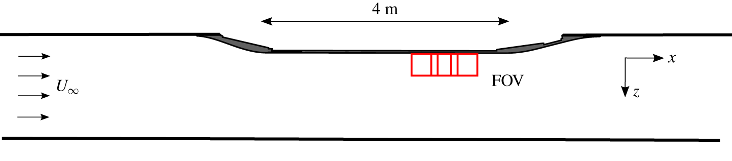
 $40~\text{m}~\text{s}^{-1}$ can be obtained. The boundary layer of interest develops along the side wall of the test section, where a model is installed with the intent to investigate turbulent boundary layers subjected to strong adverse pressure gradients (Novara et al. Reference Novara, Schanz, Reuther, Kähler and Schröder2016; Reuther & Kähler Reference Reuther and Kähler2018; Bross, Fuchs & Kähler Reference Bross, Fuchs and Kähler2019). The model itself consists of two S-shaped deflections and a 4 m long flat plate part, which allows the flow to adequately recover from the upstream pressure gradient history before entering the well-defined adverse pressure gradient region with a continuously change in pressure. This work solely focuses on the flat plate region because of the global scientific interest in flat plate boundary layer research with zero pressure gradient. Static pressure measurements conducted over the model reveal a distinct zero pressure gradient at the location of the investigated field of view (FOV). Figure 1 shows a schematic of the boundary layer experiment and the experimental set-up. The coordinate system
 $x$,
 $y$ and
 $z$ refers to the streamwise, spanwise and wall-normal directions with
 $U$,
 $V$ and
 $W$ being the related velocity components.
Large-scale two-component PIV was performed to resolve the boundary layer in the zero pressure gradient region at a friction Reynolds number of  $Re_{\unicode[STIX]{x1D70F}}\approx 9300$. This corresponds to an inflow velocity of
 $23~\text{m}~\text{s}^{-1}$. Due to the contraction, the free stream velocity at the model is approximately
 $28~\text{m}~\text{s}^{-1}$. To observe the particle displacement in the measurement plane, schematically shown in figure 1, three PCO sCMOS cameras (image sensor size:
 $2560\times 2160~\text{pixels}$) equipped with 50 mm lenses from Carl Zeiss were installed on top of the test section, resulting in a total FOV of
 $0.8~\text{m}\times 0.24~\text{m}$. To achieve a homogeneous seeding density in the test section of the wind tunnel, DEHS particles, with a mean size of approximately
 $1~\unicode[STIX]{x03BC}\text{m}$ (Kähler, Sammler & Kompenhans Reference Kähler, Sammler and Kompenhans2002), were added to the flow in the intake tower of the blow-down wind tunnel by using a PIVTEC seeding generator. Illumination of the tracer particles was realized by means of a Spectra Physics Quanta-Ray PIV 400 laser with a light sheet thickness of approximately 1 mm at the measurement location. To avoid undesirable diffuse reflections at the wall, the flat aluminium plate was polished and the propagation direction of the laser was parallel to the model surface (Kähler, Scholz & Ortmanns Reference Kähler, Scholz and Ortmanns2006).
To obtain converged statistical quantities, 20 000 double-frame images were recorded. Single large-scale PIV recordings were evaluated using iterative multipass window-correlation approaches with image deformation (Raffel et al. Reference Raffel, Willert, Scarano, Kähler, Werely and Kompenhans2018). The final interrogation window size is  $16\times 16~\text{pixels}$ and the overlap 50 %. The resulting spatial resolution is approximately
 $0.007\unicode[STIX]{x1D6FF}$.
Schematic of the boundary layer model and the experimental set-up (top view).

3 Mean velocity profiles
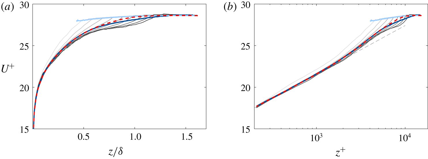
Conditioned streamwise mean velocity profiles  $\overline{U}_{t}$ (dark blue line) and
 $\overline{U}_{nt}$ (light blue line) scaled in outer and inner units. Red dashed line indicates the non-conditioned mean velocity
 $\overline{U}$. Grey lines represent
 $\tilde{U}$ for
 $\unicode[STIX]{x1D6FF}_{i}=0.5{-}1.2\unicode[STIX]{x1D6FF}$ in intervals of 0.1. Light grey lines reflect small instantaneous TNTI heights while dark grey lines represent larger ones.

To characterize turbulent flows, the mean velocity profile is most important. By time averaging hot-wire measurements, Millikan (Reference Millikan1938) already found the existence of a logarithmic layer in the mean streamwise velocity profile in the inner region of the boundary layer where the flow is always turbulent and Coles (Reference Coles1956) observed the development of a wake-like outer flow region as a consequence of the intermittent region measured by Klebanoff (Reference Klebanoff1955). As the height of the boundary layer varies strongly in time at a specific streamwise location, it is already evident that the flow velocity must fluctuate around the mean velocity as the gradient of the flow profile depends directly on the boundary layer height. Therefore, the question arises how does the mean flow profile look like for different boundary layer heights at a certain streamwise location?
To obtain these conditioned mean velocity profiles, the TNTI needs to be first detected in each of the instantaneous two-dimensional PIV measurements. As the focus of this study is more macroscopic than microscopic, the homogeneity criterion by Reuther & Kähler (Reference Reuther and Kähler2018) is applied due to its ability to detect the large-scale shape of the TNTI with sufficient spatial resolution. In comparison to other TNTI detection techniques (Holzner et al. Reference Holzner, Liberzon, Guala, Tsinober and Kinzelbach2006; Anand, Boersma & Agrawal Reference Anand, Boersma and Agrawal2009; Chauhan et al. Reference Chauhan, Philip, de Silva, Hutchins and Marusic2014), this criterion focuses on the characteristics of the non-turbulent flow, its homogeneity. To locally measure the homogeneity of the flow, the spatial standard deviation of the streamwise velocity is calculated within a sampling window of appropriate size. The deviations from the real TNTI location are relatively small and have only a negligible effect on the statistical evaluation, although small bias errors may occur due to spatial averaging as discussed in Reuther & Kähler (Reference Reuther and Kähler2018).
Based on a subdivision of instantaneous velocity fields into turbulent and non-turbulent flow regions, conditioned mean velocity profiles were obtained. By locally taking into account the number of the respective turbulent and non-turbulent velocities considered,  $\overline{U}_{t}$ and
 $\overline{U}_{nt}$ were calculated. Here, the indices ‘
 $t$’ and ‘
 $nt$’, respectively, refer to the kind of flow state (‘
 $t$’, turbulent; ‘
 $nt$’, non-turbulent). Moreover, the mean velocity was conditioned with the TNTI height
 $$\begin{eqnarray}\tilde{U} (x,z,\unicode[STIX]{x1D6FF}_{i})=\langle U(x,z,t)\mid \unicode[STIX]{x1D6FF}(x,t)=\unicode[STIX]{x1D6FF}_{i}\rangle ,\end{eqnarray}$$
where  $\unicode[STIX]{x1D6FF}(x,t)$ is the boundary layer height determined independently and
 $\unicode[STIX]{x1D6FF}_{i}$ is a prescribed boundary layer height. Figure 2 presents the Reynolds averaged velocity profile
 $\overline{U}$ scaled in outer and inner units (red line), but also the ones conditioned to the flow state (
 $\overline{U}_{t}$, dark blue line;
 $\overline{U}_{nt}$, light blue line) and the TNTI height (
 $\tilde{U}$, grey line), for a fixed streamwise location. Considering the profiles conditioned to each kind of the flow state, the figure reveals that the laminar potential flow regions maintain their momentum to a large extent (light blue line). The decrease at
 $z/\unicode[STIX]{x1D6FF}=0.5$ relative to the free stream velocity is slightly above 2 %. In addition, it is obvious that the velocity profile determined only from the turbulent parts of the boundary layer (dark blue line) shows a pronounced wake layer which deviates slightly from the conventional Reynolds averaged velocity profile. This implies that the non-turbulent flow regions transfer their momentum to the turbulent regions when they are entrained into a turbulent boundary layer region due to intermittency. In effect the turbulent flow gains momentum due to the action of entrainment of irrotational high momentum fluid. In other words, due to the interaction between entrained laminar flow regions and turbulent bulges, energy is transferred from the laminar outer motion to the turbulent regions of the boundary layer. Finally, it should be emphasized that these observations agree well with analysis of direct numerical simulation (DNS) data at
 $Re_{\unicode[STIX]{x1D703}}\approx 1550$ presented by Jiménez et al. (Reference Jiménez, Hoyas, Simens and Mizuno2010), which indicates that the applied TNTI detection approach is well suited for an adequate conditioned statistical analysis.
A consideration of  $\tilde{U} (\unicode[STIX]{x1D6FF}_{i})$ reveals that the logarithmic region of the boundary layer is barely affected by the TNTI height, see figure 2. Smaller discrepancies are observed only for
 $\unicode[STIX]{x1D6FF}_{i}=0.5$. This implies that the constants
 $\unicode[STIX]{x1D705}$ and
 $B$ of the log-law are not dependent on
 $\unicode[STIX]{x1D6FF}_{i}$. Only for
 $\unicode[STIX]{x1D6FF}_{i}<0.5\unicode[STIX]{x1D6FF}$, may the slope coefficient and the intercept change. But as this flow state is very rare (less than 0.25 % of all time steps) the integral effect on
 $\unicode[STIX]{x1D705}$ and
 $B$ is negligible. However, almost directly above the log-layer region the individual profiles start to significantly deviate from the Reynolds averaged mean velocity profile due to the fact that the velocity at the outermost location is approximately
 $U_{\infty }$. Interestingly, all profiles show almost identical strong velocity gradients
 $\text{d}U/\text{d}z$ at the TNTI and a characteristic step change in streamwise velocity. This causes the well known vortical vorticity jump at the TNTI which is associated with nibbling process (Philip, de Silva & Marusic Reference Philip, de Silva and Marusic2014) that entrains laminar fluid in the turbulent flow on small scales (Reuther & Kähler Reference Reuther and Kähler2018). Finally, velocity profiles for
 $\unicode[STIX]{x1D6FF}_{i}\geqslant 1.1$ indicate that a blockage by turbulent bulges can induce an acceleration of the potential flow in TNTI proximity as shown in figure 2. As a result,
 $\tilde{U}$ shows a slightly decreasing streamwise velocity beyond the TNTI which is associated with an increase in static pressure. On the other hand, if the potential flow streamlines are curved due to the presence of a bulge, the static pressure is slightly reduced in the outer flow due the centrifugal forces acting on the fluid elements following the curved streamlines. This pressure difference results in an upward motion of the bulges. In effect this can be considered as one mechanism that causes the boundary layer to grow in the wall-normal direction.
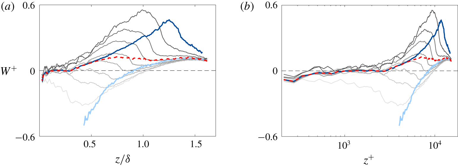
Figure 3 illustrates the equivalent conditioned wall-normal velocities  $\overline{W}_{t}$,
 $\overline{W}_{nt}$ and
 $\tilde{W}$. Inside the turbulent regime, a positive wall-normal velocity
 $\overline{W}_{t}$ is observed on average over almost the entire boundary layer. In effect, rotational fluid diffuses into the potential flow region and extends its wall-normal domain in the streamwise direction. Also, as result the potential flow shows a tiny positive velocity
 $\overline{W}_{nt}$ in the outer region due to the displacement effect through the boundary layer growth. However, in the intermittent region (
 $z/\unicode[STIX]{x1D6FF}<0.8$), results indicate on average the occurrence of strong motions towards the wall in the laminar flow region. Here, a more detailed view of the dynamics is obtained when considering
 $\tilde{W}(\unicode[STIX]{x1D6FF}_{i})$ which shows again that the inner turbulent region is barely affected by the TNTI height. Here, relatively small wall-normal velocities are found on average. Above the logarithmic layer, however, the profiles show a significant impact of the TNTI height. For
 $\unicode[STIX]{x1D6FF}_{i}>0.8\unicode[STIX]{x1D6FF}$, a strong increase in
 $\tilde{W}$ is observed in the inner intermittent region, whereas a drastic decrease is found prior to the TNTI. On the other hand, if the instantaneous TNTI height is low (
 $\unicode[STIX]{x1D6FF}_{i}<0.7\unicode[STIX]{x1D6FF}$), negative wall-normal velocities up to
 $z/\unicode[STIX]{x1D6FF}\approx 1$ are found for
 $\tilde{W}$. With respect to
 $\tilde{U}$, this implies that turbulent sweep or Q4 events, which transfer high momentum fluid towards the wall, are strongly correlated with a low TNTI height if the traditional Reynolds decomposition is applied.
Conditional wall-normal mean velocity profiles  $\overline{W}_{t}$ (dark blue line) and
 $\overline{W}_{nt}$ (light blue line) scaled in inner and outer units. Red dashed line indicates the non-conditioned mean velocity
 $\overline{W}$. Grey lines represent
 $\tilde{W}$ for
 $\unicode[STIX]{x1D6FF}_{i}=0.5{-}1.2\unicode[STIX]{x1D6FF}$ in intervals of 0.1. Light grey lines reflect small instantaneous TNTI heights while dark grey lines represent larger ones.

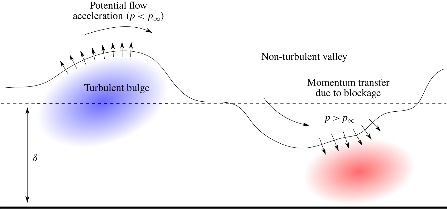
Schematic of the TNTI kinematics of a zero-pressure gradient turbulent boundary layer. Blue/red colour indicates regions where ejection/sweep events are expected if the traditional Reynolds decomposition is applied.

The discussed flow dynamics in TNTI proximity are summarized in figure 4. In the valley regions between the bulges the opposite process seems to happen than happened in the hill region. Due to the curved streamlines of the potential flow, the static pressure is increased. This induces a flow towards the wall as indicated by the arrows in the valley region in figure 4. This process is essential for maintaining the spread of the intermittent region with streamwise direction. On the other hand, it is evident that the high momentum potential flow in the valley region is blocked by the bulge located in the downstream direction. Therefore, a momentum transfer takes place from non-turbulent to the turbulent flow regions, which also explains the slight momentum decrease of the non-turbulent regions with wall proximity shown in figure 2. Furthermore, the interaction pushes the bulges forward on the back side, which gives them a typical asymmetric shape often observed in the literature (Falco Reference Falco1977; Wallace Reference Wallace2013). For a deeper analysis of the dynamics in TNTI proximity, the conditioned fluctuating velocities must be considered. However, this requires an analysis of the influence of the decomposition method as the decomposition method can strongly bias the observations.
4 Decomposition approaches
In this section, the three decomposing techniques which are analysed in the following are briefly outlined. First, the traditional Reynolds decomposition by Reynolds (Reference Reynolds1895) is considered, as this approach is usually considered as a kind of gold standard. Second, the TNTI height based decomposition by Kwon et al. (Reference Kwon, Hutchins and Monty2016) is discussed. Third, a zonal decomposition concept is considered, which prevents a contamination by the potential flow field even in the case of complex flows along curved walls with unsteady flow separation, as no averaging is required to obtain converged flow statistics.
4.1 Reynolds decomposition
The Reynolds decomposition is the most simple method of decomposing a turbulent quantity fluctuating around a mean value. Depending upon the definition of the mean (Herget Reference Herget1985), the approach can be simply viewed as a scale decomposition (Adrian, Christensen & Liu Reference Adrian, Christensen and Liu2000). The mean is in general determined by time averaging in the case of flows that are stationary on average or by ensemble averaging for flows that are transient in time. Hence, fluctuating velocities are obtained as follows:
 $$\begin{eqnarray}U(x,z,t)=\overline{U}(x,z)+u(x,z,t),\end{eqnarray}$$
where  $U$ is the instantaneous velocity,
 $\overline{U}$ the local mean and
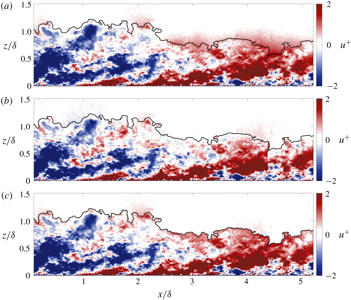
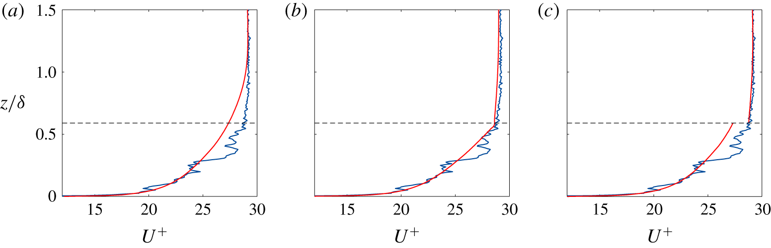
 $u$ the fluctuating velocity component. By subtracting the temporal mean from the total velocity, fluctuating velocities are obtained. Applying this decomposition approach to experimental data acquired by means of the large-scale PIV measurement is shown in figure 5. Here, the instantaneous TNTI is indicated by the black solid line. To illustrate the effect of the decomposition method on the fluctuation velocity in more detail, figure 6 shows an exemplary instantaneous velocity profile at
 $x/\unicode[STIX]{x1D6FF}=4.5$ in combination with the respective mean velocity profile. Fluctuating velocity magnitudes are represented by the displacement of the curves. From a visual inspection of the fluctuating velocity field, the crucial deficiency of this approach becomes obvious, i.e. laminar flow regions are considered as turbulent due to the fluctuations of the TNTI. In other words, strong positive virtual turbulent fluctuations are observed in the potential flow regions where the instantaneous TNTI height is low. The reason for these strong non-turbulent fluctuating velocities is simple. While ensemble averaging results in an approximate mean quantity of
 $0.94\overline{U}/U_{\infty }$ at
 $z/\unicode[STIX]{x1D6FF}\approx 0.6$ for instance, non-turbulent valleys on average feature streamwise velocities close to the free stream velocity (
 $0.97\overline{U}/U_{\infty }$) at this specific location, as there is only a small loss of kinetic energy due to the mentioned interaction of the laminar flow regions with the turbulent bulges. Consequently, the traditional Reynolds decomposition leads to virtual turbulent fluctuations in the potential flow regime exclusively due to the unsteadiness of the TNTI. Therefore, higher-order statistics, which should purely represent the fluctuations attributable to turbulence, are biased by laminar flow regions. Furthermore, apparent extreme turbulent events in view of the fluctuation magnitude appear in the valley region due to the presence of laminar flow regions. This illustrates how the Reynolds decomposition can mislead the interpretation of the results. To characterize the turbulent motion in a more physical manner, new decomposition approaches are required that take the characteristic intermittent behaviour into account.
Streamwise velocity fluctuations obtained when applying (a) the traditional Reynolds decomposition, (b) the boundary layer height based decomposition and (c) the zonal decomposition. Black line indicates TNTI.

Effect of the decomposition approach on the fluctuation velocities at  $x/\unicode[STIX]{x1D6FF}=4.5$: (a) Reynolds decomposition, (b) boundary layer height based decomposition and (c) zonal decomposition. Instantaneous velocity is represented by the blue line while red lines show respective mean velocities. Fluctuating velocity magnitudes are represented by the displacement of the curves. Dotted line indicates the instantaneous boundary layer height
 $\unicode[STIX]{x1D6FF}_{i}$.

4.2 Decomposition based on the boundary layer height
In order to ensure that the TNTI fluctuations do not affect the fluctuating velocity estimation, Kwon et al. (Reference Kwon, Hutchins and Monty2016) proposed a decomposition approach based on the local instantaneous boundary layer height. This method can be expressed as follows:
 $$\begin{eqnarray}U(x,z,t)=\tilde{U} (x,z,\unicode[STIX]{x1D6FF}_{i})+u(x,z,t).\end{eqnarray}$$
With respect to the instantaneous TNTI location and the discretized conditional mean velocities, the local streamwise velocities were decomposed according to equation (4.2) in the following. From figures 5 and 6, it becomes obvious that the variations in non-turbulent fluctuating velocity are drastically reduced when taking into account the boundary layer height variations. Further, it is evident that the fluctuating velocities within the turbulent regime change relative to these obtained using the Reynolds decomposition. In principle, if the local instantaneous TNTI height is large ( $z/\unicode[STIX]{x1D6FF}>0.9$), fluctuations are primarily shifted to more negative values. In contrast, if the height is small (
 $z/\unicode[STIX]{x1D6FF}<0.8$), fluctuations are predominantly shifted to more positive values as illustrated in figure 2. This is clear as the flow gradients become steeper with decreasing thickness of the turbulent region.
Nevertheless, this promising method also comes with some drawbacks. First of all, non-physical step changes in the streamwise direction can occur if the boundary layer height exhibits rapid changes in the streamwise direction, as the corresponding mean velocity profiles differ strongly. This holds in particular if the instantaneous TNTI height is small as discrepancies in  $\tilde{U}$ exist over a larger wall-normal domain. Such an event is observed at
 $x/\unicode[STIX]{x1D6FF}\approx 4.35$ in figure 5, resulting in a clear cutoff of the large-scale motion. Second, a strong increase in streamwise velocity fluctuation is observed in the protruding parts, where Kwon et al. (Reference Kwon, Hutchins and Monty2016) suggests a fluctuating velocity computation using the zonal mean velocity (Kovasznay et al. Reference Kovasznay, Kibens and Blackwelder1970). Finally, it should be emphasized that this technique is difficult to apply for wall-bounded flows featuring stronger Reynolds number variations due to the curvature of the model or pressure gradients and it is not applicable to flows that are transient on average as no mean velocity can be estimated reliably. As a tremendous number of independent vector fields are required to obtain statistically converged mean quantities, Kwon et al. (Reference Kwon, Hutchins and Monty2016) already assumes the Reynolds number variation influence to be small in a canonical flat plate boundary layer as a compromise and considers the full streamwise length for conditional mean quantity computation.
4.3 Zonal decomposition
In order to avoid biasing due to virtual turbulent fluctuations caused by strong boundary layer height variations, even in flows featuring strong Reynolds number variations, a conditional averaging technique, which has been so far only applied to single point measurements by Antonia (Reference Antonia1972), Hedley & Keffer (Reference Hedley and Keffer1974) and Kovasznay et al. (Reference Kovasznay, Kibens and Blackwelder1970), is suitable. Unlike conventional averaging, this technique averages flow quantities only for the time the flow is either turbulent or non-turbulent. Based on the resulting separated ‘zonal’ mean velocities, the local velocity is decomposed with respect to its flow state
 $$\begin{eqnarray}U_{t}(x,z,t)=\overline{U}_{t}(x,z)+u_{t}(x,z,t)\quad \wedge \quad U_{nt}(x,z,t)=\overline{U}_{nt}(x,z)+u_{nt}(x,z,t).\end{eqnarray}$$
Considering the respective mean velocities discussed above, it is apparent that the fluctuating velocities in the intermittent region change significantly with respect to the traditional Reynolds decomposition if the flow is non-turbulent. On the other hand, deviations are comparatively small at locations where the flow is turbulent. In effect, velocity fluctuations in the non-turbulent region are shifted to more negative values with decreasing wall distance, while in the turbulent region they are shifted to slightly more positive values with increasing intermittency frequency. Note, in contrast to the decomposition approach by Kwon et al. (Reference Kwon, Hutchins and Monty2016), mean quantities are only wall distance dependent and boundary layer height independent.
Through the application of this zonal decomposition approach, a continuous fluctuating velocity distribution is found in the turbulent region as shown figure 5(c). From the figure, it is further evident that extended regions of virtual turbulent fluctuations are not present. Only some local virtual turbulence regions are present due to measurement noise. With respect to figures 5 and 6, it is striking that the zonal decomposition results in a strong jump in fluctuating velocity at the TNTI. This occurs in particular if the boundary layer height is low. Similar but slightly less amplified fluctuations are also found for the Reynolds approach in proximity to the TNTI. However, due to the virtual turbulence in the potential flow, no step change in fluctuating velocity occurs at the TNTI. In contrast, when applying the boundary layer height based decomposition, a smooth increase in fluctuating velocity is typically found at the TNTI. Hence, the question arises if these strong fluctuation velocities observed in the zonal decomposition case at the TNTI are an artefact of the boundary layer height variations or is it a characteristic physical feature that leads to a vorticity jump at the TNTI? As the height dependent mean velocity exhibits a jump at the TNTI, which leads to a vorticity peak at the interface, the jump appears as a turbulent fluctuation. Therefore, a significant turbulence level right at the TNTI seems to be physically possible.
5 Decomposition effect on single point turbulence statistics
In this section, the effect of intermittency on single point statistics is outlined. First, probability density functions of streamwise velocity fluctuation are considered. Second, the one-dimensional average magnitude of velocity fluctuations is studied as this quantity has been presented in several studies in the past to characterize turbulent boundary layers. Third, joint probability density functions (j.p.d.f.s) are investigated to analyse the anisotropy of fluctuations under the different decomposition techniques.
5.1 Velocity fluctuation probability density functions
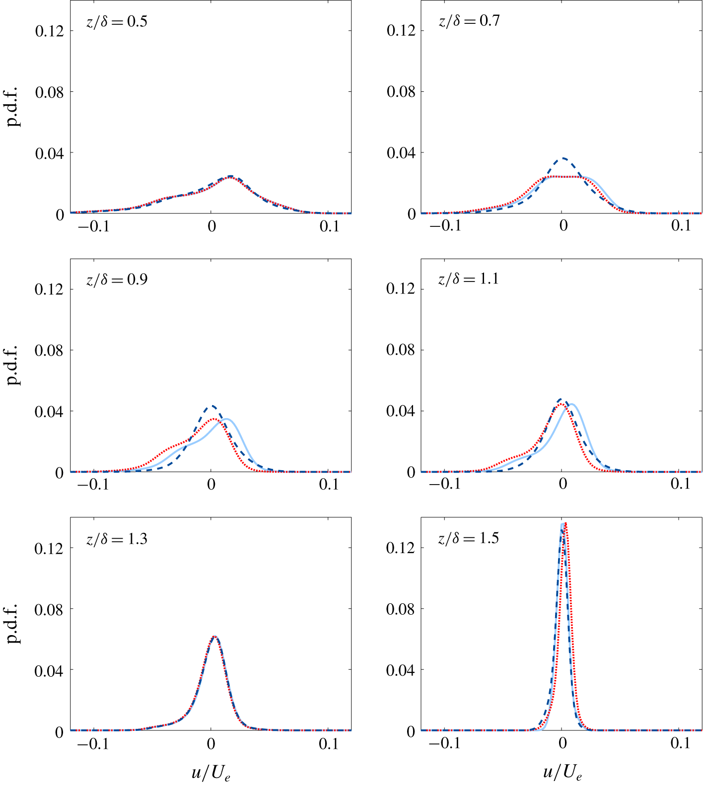
Probability density function of turbulent streamwise fluctuating velocities using different decomposition approaches for  $x_{0}=0.2~\text{m}$ and
 $0.5\leqslant z/\unicode[STIX]{x1D6FF}\leqslant 1.5$. Dotted (red) lines indicate results obtained when applying the traditional Reynolds decomposition while dashed (dark blue) and solid (light blue) lines represent results obtained using decomposition based on the boundary layer height and the zonal decomposition, respectively.

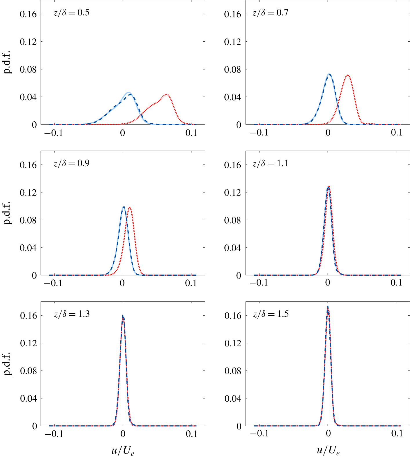
Probability density function of non-turbulent streamwise fluctuating velocities using different decomposition approaches for  $x_{0}=0.2~\text{m}$ and
 $0.5\leqslant z/\unicode[STIX]{x1D6FF}\leqslant 1.5$. Dotted (red) lines indicate results obtained when applying the traditional Reynolds decomposition while dashed (dark blue) and solid (light blue) lines represent results obtained using decomposition based on the boundary layer height and the zonal decomposition, respectively.

Based on a large set of 20 000 independent double-frame images, probability density functions (p.d.f.s) of streamwise velocity fluctuations were calculated for the individual decomposition techniques to visualize the differences in fluctuating velocity distribution. Figures 7 and 8 illustrate the approximation of the p.d.f.s of turbulent and non-turbulent streamwise fluctuating velocities using a bar width of  $0.05~\text{m}~\text{s}^{-1}$ for several wall-normal locations.
For the case of turbulent fluctuations shown in figure 7, a good agreement between the respective p.d.f.s under the different decomposition techniques is found in the lower half of the boundary layer. This suggests that the intermittency effect is rather low in the region  $z/\unicode[STIX]{x1D6FF}\leqslant 0.5$ and the impact of non-turbulent flow regions between
 $0.4\leqslant z/\unicode[STIX]{x1D6FF}\leqslant 0.5$ on single point statistics is negligibly small. Figure 2 confirms this result up to
 $z/\unicode[STIX]{x1D6FF}\approx 0.5$ as the mean velocity profiles of the different decomposition approaches almost fall on top of each other, except for a small number of extreme events where
 $\unicode[STIX]{x1D6FF}_{i}<0.6\unicode[STIX]{x1D6FF}$. Due to the low occurrence frequency, the impact of these events on statistically averaged quantities is negligible. As the intermittency effect increases, obvious deviations become visible. Due to the significant changes of the mean quantity shown in figure 2, the p.d.f.s representing the zonal decomposition show a pure shift without an effect on the distribution’s shape in the intermittent region with respect to the Reynolds decomposition. In contrast, for the case of the adapting boundary layer height based mean quantity, the p.d.f.s representing the decomposition by Kwon et al. (Reference Kwon, Hutchins and Monty2016) show a distinct change in distribution shape. Here, a narrower spectrum including a distinct Gaussian distribution is found as one would expect in a turbulent regime.
For probability density functions representing the non-turbulent fluctuations shown in figure 8, it can be seen that the choice of method has a negligible influence in regions where turbulent bulges occur less frequently ( $z/\unicode[STIX]{x1D6FF}\geqslant 1$). As a result of the low frequency of occurrence, the non-turbulent potential flow is barely affected, which in turn results in a narrow spectrum of the p.d.f.s representing the free stream turbulence along with the uncertainty of the PIV measurement. However, with decreasing
 $z/\unicode[STIX]{x1D6FF}$ the spectrum of non-turbulent fluctuations becomes wider as a result of the blockage by turbulent bulges. For the Reynolds decomposition case, the p.d.f.s show a significant shift to more positive values with increasing wall proximity. This is due to the non-physical positive fluctuating velocities associated with the TNTI fluctuations. On the other hand, the alternative decomposition methods result in an almost identical non-turbulent fluctuating velocity distribution over the entire intermittent region. For the innermost location considered, the p.d.f.s show a negative skewness. It cannot be excluded that this is associated with the TNTI detection uncertainty or the low convergence of the p.d.f. for small
 $z/\unicode[STIX]{x1D6FF}$. As the occurrence frequency of irrotational fluid decreases towards the wall, more than 20 000 independent PIV measurements to obtain converged results for this quantity.
5.2 Turbulence intensities and relaxation times
Apart from its necessity to validate numerical turbulence models (Knopp et al. Reference Knopp, Novara, Schanz, Schülein, Schröder, Reuther and Kähler2018), higher-order moments of turbulent fluctuations are essential for the characterization of turbulent flows. In the past, nearly all studies applied temporal averaging over the respective fluctuating components without considering the intermittent behaviour of turbulent boundary layers. To our knowledge only Jiménez et al. (Reference Jiménez, Hoyas, Simens and Mizuno2010) analysed mean statistics conditioned to the TNTI systematically.
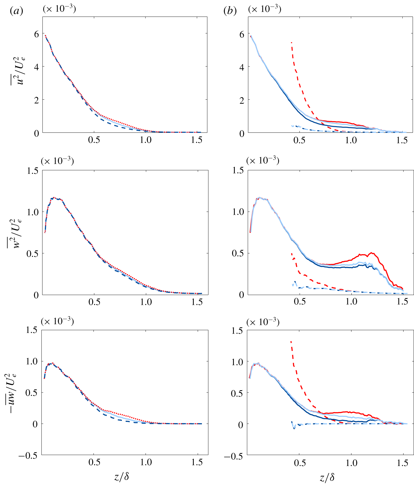
Figure 9 demonstrates the turbulence intensities for the present data set. Here, the conventional averages are illustrated in panel (a) and conditional turbulent and non-turbulent ones in panel (b). For a better representation of the method’s deviations, turbulence intensities are scaled in outer units, i.e. by means of the edge velocity obtained at  $\unicode[STIX]{x1D6FE}=0.3$. If the traditional Reynolds decomposition approach is applied, a significant increase in turbulent kinetic energy is observed in the irrotational fluid regions with decreasing wall distance due to the virtual turbulence. In contrast, when considering the unsteadiness of the TNTI during decomposition, this non-turbulent energy contribution is removed to a great extent. This holds for both the TNTI height based and the zonal decomposition approaches. When exclusively considering the turbulent flow parts, the method’s differences in streamwise turbulence intensity are significantly smaller but visible. The largest streamwise turbulence intensities in the intermittent region are found for the Reynolds approach. Due to the shift to more positive values, the zonal decomposition shows slightly reduced turbulence intensities. A further reduction in turbulence intensities is observed when the TNTI height based decomposition is applied. The difference between the height and zonal approach is predominantly caused by the fact that the near TNTI region is treated differently. As a result of these observations, the conventional profile is losing its little bump in the intermittent region as shown in figure 9.
Turbulence intensities under the traditional Reynolds decomposition (red), the boundary layer height based decomposition (dark blue) and the zonal decomposition (light blue). Unconditioned results are presented on the left-hand side, while results conditioned to the turbulent (solid lines) and non-turbulent flow state (dashed lines) are shown on the right-hand side.

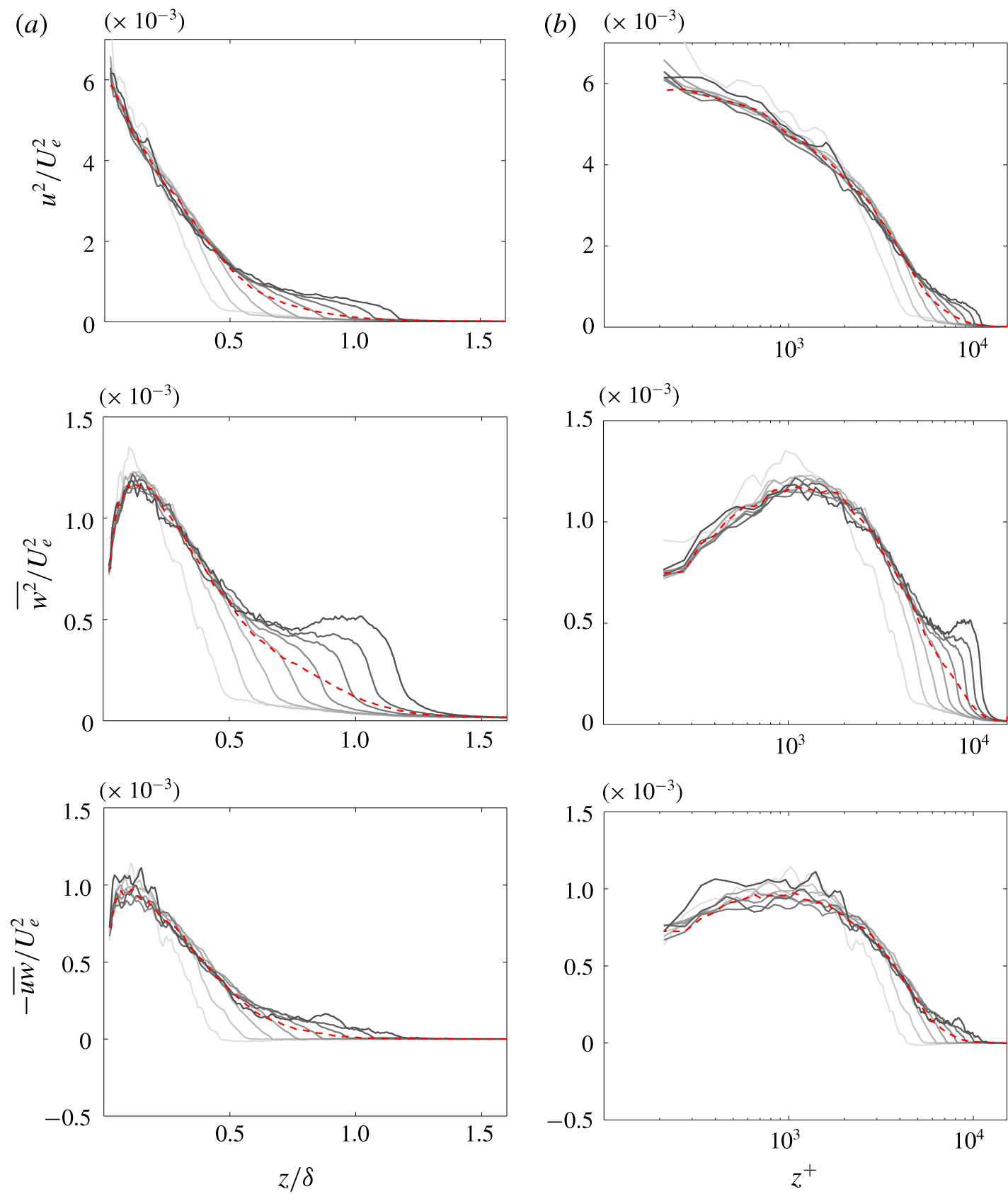
Turbulence intensities under the boundary layer height based decomposition in inner (b) and outer (a) scaling for  $\unicode[STIX]{x1D6FF}_{i}=0.5{-}1.2\unicode[STIX]{x1D6FF}$ in intervals of 0.1. Light grey lines reflect small instantaneous TNTI heights while dark grey lines represent larger ones. Dashed red line indicates the conventional average.

For a comprehensive view, wall-normal velocities were also decomposed according to the conditional mean velocities (either  $\tilde{W}(x,z,\unicode[STIX]{x1D6FF}_{i})$ or
 $W_{t}(x,z)/W_{nt}(x,z)$). Figure 9 shows the resulting Reynolds normal and shear-stress turbulence intensities. With respect to
 $\overline{w^{2}}$, again a significant reduction in non-turbulent kinetic energy is observed for the alternative decomposition methods. For the mean quantities determined only on the turbulent parts, the results show the expected peak in the intermittent region but also reveal a plateau over a wide wall-normal range of the intermittent region. For the simple Reynolds decomposition, interestingly an outer peak evolves.
By conditioning turbulence intensities, Jiménez et al. (Reference Jiménez, Hoyas, Simens and Mizuno2010) found the rotational flow state to feature a shear-stress turbulence intensity  $-\langle uw\rangle <0$ for
 $z/\unicode[STIX]{x1D6FF}>0.6$. However, the present data indicates that this quantity is positive everywhere in the rotational regime for the zero pressure gradient turbulent boundary layer considered here. Moreover, results reveal that the irrotational fluid does not contribute to turbulence production (
 $-\langle uw\rangle \unicode[STIX]{x2202}U/\unicode[STIX]{x2202}z$) if the intermittent behaviour is considered. This is in good agreement with the common understanding of the potential flow.
To investigate the effect of the boundary layer topology, the turbulence intensities were conditioned to the instantaneous boundary layer height  $\unicode[STIX]{x1D6FF}_{i}$. The results are shown in figure 10. Consistent to previous observation,
 $\unicode[STIX]{x1D6FF}_{i}$ has almost no influence on the statistical quantities in the fully turbulent region below
 $z/\unicode[STIX]{x1D6FF}<0.4$. However, in the intermittent region again strong deviations can be observed. In general, a sudden change in turbulence intensity is observed in proximity to the TNTI. This holds for
 $\overline{u^{2}}$ and
 $\overline{w^{2}}$, although a slight shift in step change wall-normal location is observed. Beyond this location, turbulence magnitudes are found to be relatively small and further decrease with wall distance or turbulent bulge interaction, respectively. With respect to the turbulent regime, figure 10 reveals that even strongly pronounced turbulent bulges exhibit a remarkable turbulence intensity level (
 $\overline{u^{2}}$ and
 $\overline{w^{2}}$) before showing a drastic decrease in TNTI proximity. The magnitudes of the shear stress turbulence intensities show that the gradient of
 $\overline{uw}$ at the TNTI rises with decreasing
 $\unicode[STIX]{x1D6FF}_{i}$. In addition, the mean streamwise flow profile becomes steeper with decreasing
 $\unicode[STIX]{x1D6FF}_{i}$ which implies that the turbulence production reaches its maximum when
 $\unicode[STIX]{x1D6FF}_{i}$ is minimal. However, as very small
 $\unicode[STIX]{x1D6FF}_{i}$ are rare, it is likely that most of the total turbulence production takes place at moderate
 $\unicode[STIX]{x1D6FF}_{i}$.
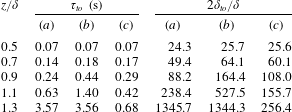
This analysis leads to another important implication. If the flow is somehow disturbed the question arises, how long does it takes to reach equilibrium state again? According to Sillero, Jiménez & Moser (Reference Sillero, Jiménez and Moser2013), the flow is assumed to relax to equilibrium after  $2\unicode[STIX]{x1D70F}_{to}$, where
 $\unicode[STIX]{x1D70F}_{to}$ is the eddy turnover time based on the turbulent shear stress
 $$\begin{eqnarray}\unicode[STIX]{x1D70F}_{to}=\frac{z}{2\sqrt{\overline{uw}}}.\end{eqnarray}$$
The corresponding turnover length  $2\unicode[STIX]{x1D6FF}_{to}$ is equal to
 $2\overline{U}(z)\unicode[STIX]{x1D70F}_{to}$. If the traditional Reynolds decomposition is applied and the non-conditioned averages are considered for
 $\overline{uw}$ and
 $\overline{U}(z)$, the eddy turnover length
 $2\unicode[STIX]{x1D6FF}_{to}$ is approximately
 $88\unicode[STIX]{x1D6FF}$ for
 $z/\unicode[STIX]{x1D6FF}=0.9$. However, the streamwise travelling distance of history effects drastically increases to
 $2\unicode[STIX]{x1D6FF}_{to}\approx 164$ if the interface height based decomposition is applied. This indicates that disturbances affect the flow even more long-lastingly than previously thought. On the other hand, an opposite effect takes place if one considers the averages conditioned to the turbulent flow state (
 $\overline{uw}_{t}$ and
 $\overline{U_{t}}(z)$). As the turbulence intensities increase and mean streamwise velocity decrease, the relaxation length scale significantly decreases to only
 $2\unicode[STIX]{x1D6FF}_{to}\approx 108\unicode[STIX]{x1D6FF}$ for
 $z/\unicode[STIX]{x1D6FF}=0.9$. Note, while the conventional approach leads to a slight underestimation of the turnover length at
 $z/\unicode[STIX]{x1D6FF}=0.9$, a drastic overestimation is observed for
 $z/\unicode[STIX]{x1D6FF}>1.1$, as shown in table 1, where
 $\overline{uw}$ is negligible small on average. These considerations can have important consequences when boundary layers are artificially tripped by using zig-zag tape, rod wires or sandpaper.
Eddy turnover time and length as a function of the wall distance  $z$ for three different approaches: (a) traditional Reynolds decomposition and non-conditioned averages, (b) boundary layer height based decomposition and non-conditioned averages and (c) boundary layer height based decomposition and conditioned averages.

5.3 Anisotropy of fluctuating velocities
So far, the one-dimensional average magnitudes of fluctuations were discussed. Next, the anisotropy of turbulent velocity fluctuations is considered which can be used as an indicator for coherent features within a turbulent boundary layer. In order to study the anisotropy, joint probability density functions of streamwise/wall-normal velocity fluctuations under the three different decomposition approaches are investigated. Strictly speaking,  $u$ and
 $w$ are a function of
 $Re_{\unicode[STIX]{x1D70F}}$ and
 $p_{x}^{+}$. Hence, to adequately resolve the local anisotropy, the fluctuating velocities need to be investigated at single streamwise locations. As this would require a tremendous number of independent velocity vector fields, the Reynolds number variation is assumed to have a negligible small impact over a short streamwise domain (0.3
 $\unicode[STIX]{x1D6FF}$) as a compromise. Furthermore, the bin sizes, the instantaneous velocity vectors were assigned to, were kept relatively large (0.005
 $U_{e}\times 0.005U_{e}$) for convergence reasons. Although j.p.d.f.s obtained by this means might suffer from slight inaccuracies, it allows one to quantitatively analyse the anisotropy of fluctuating velocities relatively well.
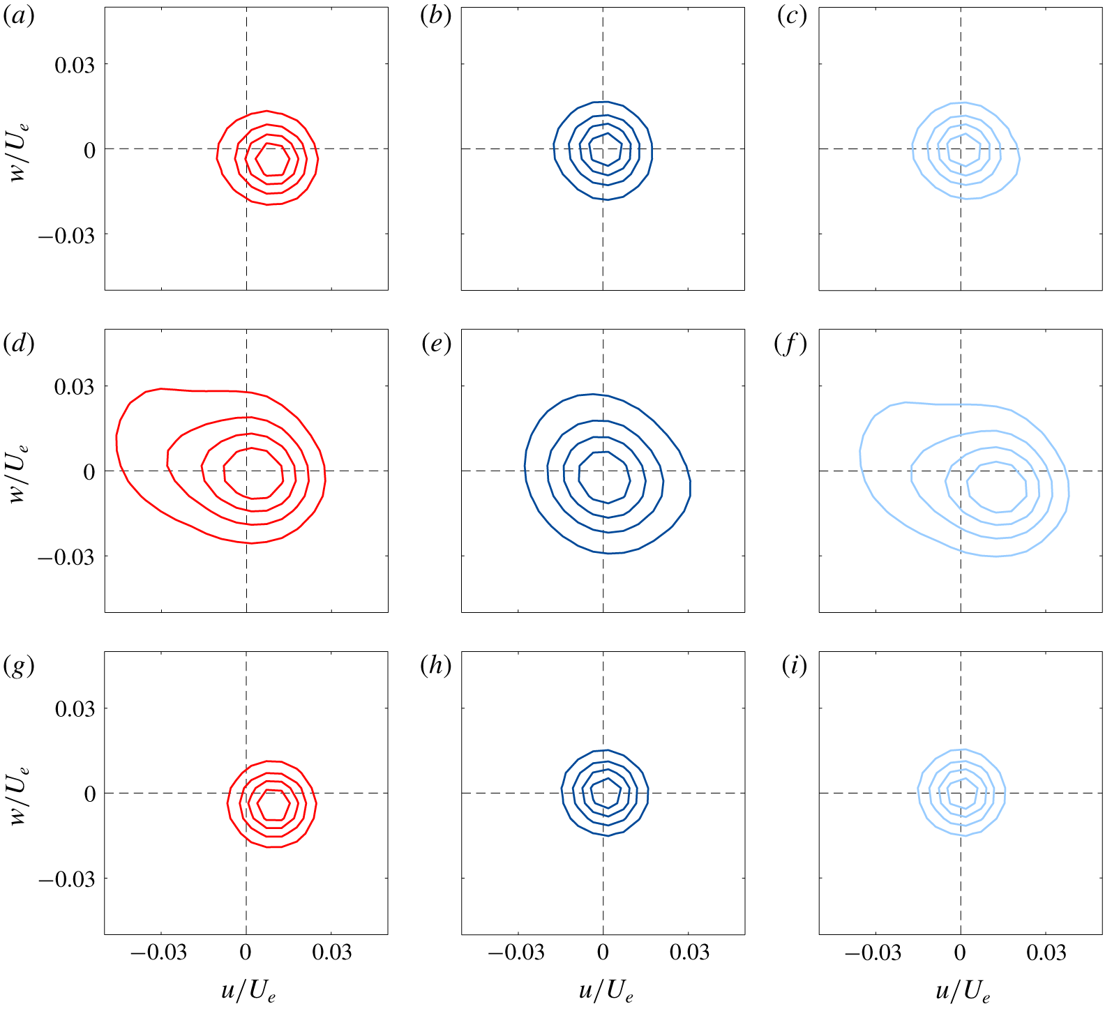
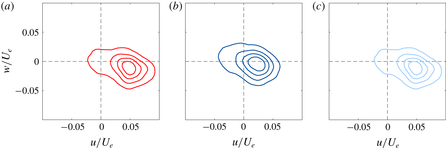
Figure 11 illustrates the unconditioned j.p.d.f.s, but also j.p.d.f.s conditioned to the turbulent (d–f) and the non-turbulent flow state (g–i) for a wall-normal location of  $z/\unicode[STIX]{x1D6FF}=0.9$. At
 $z/\unicode[STIX]{x1D6FF}=0.9$ the intermittency influence is the largest (
 $\unicode[STIX]{x1D6FE}\approx 0.5$). For wall-normal locations in the non-intermittent turbulent region, the j.p.d.f.s naturally collapse. However, as we move to the location where
 $\unicode[STIX]{x1D6FE}=0.5$, the j.p.d.f.s increasingly deviate. As the Reynolds decomposition detects erroneously the TNTI unsteadiness as turbulence, the conventional as well as the j.p.d.f. conditioned to the non-turbulent flow state indicate a non-isotropic behaviour with a high probability of Q4 events (
 $u>0$ and
 $w<0$). However, if the TNTI fluctuations are considered for total velocity decomposition, the unconditioned j.p.d.f. and the j.p.d.f. conditioned to the irrotational fluid state show a distinct isotropic behaviour. Here, only slight deviations between the alternative decomposition approaches are observed.
Unconditioned and conditioned j.p.d.f.s at  $z/\unicode[STIX]{x1D6FF}=0.9$ under the traditional Reynolds decomposition (red contours), decomposition based on the TNTI height (dark blue contours) and the zonal decomposition (light blue contours). (a,b,c) unconditioned j.p.d.f.s; (d,e,f) turbulent j.p.d.f.s; (g,h,i) non-turbulent j.p.d.f.s. Contours are shown for 0.2–0.8 in intervals of 0.2.

If only the pure turbulent j.p.d.f. is considered, the spectra of turbulent fluctuations naturally become much wider. This holds for all methods investigated. Nevertheless, significant deviations are observed due to the different ways of decomposing the total velocity. While the results using the TNTI height based decomposition indicate only a slight elliptical shape of the j.p.d.f. as known from the inner region of the boundary layer where the log-law holds (Novara et al. Reference Novara, Schanz, Reuther, Kähler and Schröder2016), j.p.d.f.s under the zonal and Reynolds decomposition show a more distorted shape towards Q2 and Q4 events. It is interesting to see that due to the shift to more positive  $u$ and more negative
 $w$, the distribution is significantly shifted towards Q4 events in the case of the zonal decomposition compared to the Reynolds decomposition. Furthermore, it can be seen that the maximum amplitude of the fluctuations in the
 $+$ and
 $-$ direction is quite similar at this
 $z/\unicode[STIX]{x1D6FF}$ location. The j.p.d.f. composed of the laminar flow regions look quite similar, while the height and zonal based distribution are symmetric with respect to the centre, the one resulting from the Reynolds decomposition approach, is shifted in accordance with the results in figure 8.
In order to verify the hypothesis that Q4 events are strongly correlated with a low TNTI height, turbulent j.p.d.f.s at  $z/\unicode[STIX]{x1D6FF}=0.4$ were conditioned to a TNTI height
 $\unicode[STIX]{x1D6FF}_{i}<0.65\unicode[STIX]{x1D6FF}$. This TNTI height corresponds to an intermittency factor
 $\unicode[STIX]{x1D6FE}$ of 0.9. Figure 12 illustrates the results for the three decomposition approaches. The figure clearly shows that the turbulent flow below a pronounced non-turbulent valley is dominated by Q4 events. Due to the fact that
 $\overline{W}_{t}\approx 0$ at this specific location as illustrated in figure 3, this indicates that high momentum fluid is transferred towards the wall. This feature holds for all decomposition methods considered.
Joint probability density functions at  $z/\unicode[STIX]{x1D6FF}=0.4$ conditioned to TNTI heights
 $\unicode[STIX]{x1D6FF}_{i}<0.65\unicode[STIX]{x1D6FF}$. Colours represent the different decomposition approach according to figure 11. Contours are shown for 0.2 to 0.8 in intervals of 0.2.

6 Decomposition effect on multipoint statistics
Analysing the turbulence intensities has revealed that a significant portion of energy is artificially added when applying the traditional Reynolds decomposition. This is in good agreement with results by Kwon et al. (Reference Kwon, Hutchins and Monty2016). By investigating the premultiplied power spectral densities of streamwise velocities, Kwon et al. (Reference Kwon, Hutchins and Monty2016) additionally found that the discrepancies on the energy distribution predominantly occur at the large-scale wavelength. These findings, in turn, suggest that the classical large-scale coherence analysis of streamwise velocity fluctuations is prone to bias errors due to the virtual turbulence.
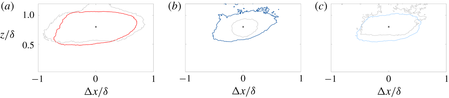
To detect the long coherent regions of high- and low-speed fluid, visualized in figure 5, and to estimate its average extent, two-point correlations (TPCs) of streamwise velocity fluctuations have been employed in a number of studies (Tomkins & Adrian Reference Tomkins and Adrian2003; Kähler Reference Kähler2004; Ganapathisumbramani et al. Reference Ganapathisumbramani, Hutchins, Hambleton, Longmire and Marusic2005; Hutchins & Marusic Reference Hutchins and Marusic2007; Lee & Sung Reference Lee and Sung2011; Rahgozar & Maciel Reference Rahgozar and Maciel2012; Bross et al. Reference Bross, Fuchs and Kähler2019). However, apart from the decomposition effects, the following crucial aspects have not been addressed in the past when performing TPCs for large-scale motion analysis: (i) due to the intermittent behaviour, the correlation point is not always located within the turbulent regime in an instantaneous PIV velocity field. Furthermore, with increasing wall distance the probability that the correlation point is located in the potential flow regions increases. (ii) It has to be taken into account that in the potential flow region the neighbouring vectors are quite homogeneous in magnitude and direction in contrast to real turbulent fluctuations. Consequently, the correlation function is systematically biased by the laminar flow regions. (iii) The reference point is correlated with the full FOV, assuming that turbulent fluctuation solely occur in the turbulent regime. However, as the Reynolds decomposition evokes virtual turbulence in the laminar region, reference points in the turbulent region might show a strong correlation with potential flow regions. Hence, due to these aspects the large-scale coherence of turbulent flow structures might not be adequately reflected. This holds in particular for reference points in the intermittent region but also when the reference point is located in the inner layer and the other correlation point is located in a region of virtual turbulence.
In order to avoid the bias errors addressed above, the effect of intermittent behaviour of wall-bound flows on spatial correlations is further considered in this section. First, individual vector fields where the correlation reference point is instantaneously located in the potential flow region were neglected for two-point correlation analysis. Second, to avoid any potential flow influence, the correlation point was solely correlated with the turbulent regime. Note, this already presupposes that the reference point is located within the turbulent region. To implement this, magnitudes of fluctuating velocities in the potential flow field were set to zero for each time step and the fraction of time the flow is turbulent was counted locally for normalization reasons.
Conditioned two-point correlation map of streamwise velocity fluctuations for  $z_{c}/\unicode[STIX]{x1D6FF}=0.8$. (a) Traditional Reynolds decomposition and the classical TPC approach, (b) TNTI height based decomposition and modified TPC approach, (c) zonal decomposition and modified TPC approach. Coloured lines indicate unconditioned TPC results while grey lines represent conditioned TPC results (
 $u>\unicode[STIX]{x1D70E}(x_{c},z_{c})$). Contours are plotted for 0.25.

To adequately investigate the intermittency effect on two-point correlation maps of streamwise velocity fluctuations, large-scale motion analysis was performed using the Reynolds, the TNTI height and the zonal decomposition for a reference point  $z_{c}/\unicode[STIX]{x1D6FF}=0.8$. Note, the TPC modifications discussed above have not been applied to the Reynolds decomposition case. The results of the unconditioned TPC analysis are shown in figure 13 by means of the coloured isolines. The comparison of the results of the individual approaches reveals that the motion’s streamwise extent in the intermittent region is significantly smaller if only turbulent flow regions are taken into account. Furthermore, it is evident that results of the two alternative decomposition approaches show a similar motion length scale if the modified TPC approach is applied. The appearance of the large-scale coherent motions, however, changes. While an application of the zonal decomposition yields a motion shape featuring a flat top due to the strong fluctuations at the TNTI, the map of two-point correlation shows an inclined motion shape even in the outer region under the TNTI height based decomposition. Note, due to the fact that the time the flow is turbulent decreases with increasing wall distance, scattering occurs in the outer region when applying the modified two-point correlation approach due to the lack of convergence.
For further investigation, TPCs were conditioned to the sign and magnitude of streamwise velocity fluctuations. In particular with respect to the turbulent large-scale motion development, only strong events were taken into account. Here, a strong event is defined, where the magnitude of streamwise velocity fluctuation exceeds the local standard deviation  $\unicode[STIX]{x1D70E}(x_{c},z_{c})$ at the reference position. As the map of streamwise fluctuating velocities changes with the decomposition approach applied, the local standard deviation slightly changes as well. However, the variation in
 $\unicode[STIX]{x1D70E}$ has no detectable impact on the two-point correlation maps of streamwise velocity fluctuations conditioned to
 $u>\unicode[STIX]{x1D70E}(x_{c},z_{c})$, which are illustrated in figure 13 (light grey lines). For a comprehensive view, it should be mentioned that conditioning to
 $u<\unicode[STIX]{x1D70E}(x_{c},z_{c})$ yields similar streamwise length scales
 $L$ for the three different TPC approaches (
 $L\approx 2.3\unicode[STIX]{x1D6FF}$). However, the impact of conditioning on
 $u>\unicode[STIX]{x1D70E}(x_{c},z_{c})$ is enormous. While the motions featuring strong positive streamwise fluctuating velocities exhibit only
 $0.45\unicode[STIX]{x1D6FF}$ for the modified TPC method case in combination with the TNTI height based decomposition, a motion size of
 $1.8\unicode[STIX]{x1D6FF}$ is found for the classical TPC method, based on a correlation threshold of 0.25. In contrast, if the modified TPC is based on fluctuations obtained using the zonal decomposition, a motion length scale of approximately
 $1\unicode[STIX]{x1D6FF}$ is detected. This result clearly illustrates how the selected decomposition approach can bias the structural features of the coherent motions in the flow. Moreover, the presented statistical analysis shows that the zonal decomposition leads to an adequate physical estimation of the turbulent flow features with coherent properties.
7 Conclusion
Reynolds decomposition is a well-established and often used approach for the statistical analysis of turbulent flows which are in a turbulent state at any time. If, however, the turbulent state is interrupted from time to time by laminar flow states, the question arises how the intermittent behaviour can be statistically treated in such that the turbulence statistics is not biased by laminar flow regions and the characteristic properties of the turbulence are represented physically correct.
In order to examine how the treatment of intermittency dynamics affects single and multipoint statistics, we have investigated the intermittent region of a flat plate turbulent boundary layer flow without pressure gradient at  $Re_{\unicode[STIX]{x1D70F}}=9300$ using three different velocity decomposition approaches. First, the well-established Reynolds decomposition approach. This approach does not distinguish between laminar and turbulent flow states at all, since the entire mean velocity profile is used to calculate the turbulent velocity fluctuations. Second, the turbulent/non-turbulent interface height based approach. This decomposition approach estimates the turbulent velocity variations by subtracting the conditioned mean velocity profile corresponding to the specific height of the boundary layer at position
 $x$ and time
 $t$. Third, the zonal decomposition approach. This calculates the turbulent velocity fluctuations at a given wall normal location based exclusively on turbulent flow statistics. In this case, the mean velocity profile is determined purely from the turbulent flow state profile and all laminar flow regions are discarded for the mean turbulent velocity profile estimation. The analysis clearly shows that each of the three decomposition approaches have their own strengths and weakness and have a significant influence on the statistical results and thus on the interpretation of the turbulent flow physics.
The results indicate that the greatest weakness of the Reynolds decomposition approach is that this method considers laminar flow areas in the intermittent flow region as turbulent fluctuations. In effect, the laminar regions strongly bias the results of the turbulence statistics. In the intermittent region  $z/\unicode[STIX]{x1D6FF}<0.5$, for example the detection rate of laminar flow areas is low, but the amplitude of the fluctuations reaches very large positive values, because the laminar flow areas retain their momentum when entrained by the turbulent motion. Therefore, the laminar flow areas appear as kind of extreme turbulent events in this region, although they do not exhibit any typical properties of turbulent flows. For this reason they can be considered as a kind of virtual turbulence which bias the statistical results to a large extent. In the range
 $z/\unicode[STIX]{x1D6FF}>0.8$, the laminar flow areas begin to dominate the statistics in two essential ways. First, the magnitude of the laminar velocity entrained into the turbulent flow region is quite similar. Second, the direction of the laminar flow regions is highly homogeneous in strong contrast to the turbulent flow regions whose velocity magnitude and direction is much more uncorrelated. Since the magnitude and direction of the velocity in the laminar flow range is quite homogeneous, the laminar flow areas significantly bias the statistical results even at lower
 $z/\unicode[STIX]{x1D6FF}$ values. This artificially increases the turbulent kinetic energy in the outer region of the boundary layer due to the virtual turbulent flow motion. The same applies to the Reynolds shear stresses and thus the production of turbulence in the outer region of the turbulent boundary layer. Therefore, the application of the traditional Reynolds decomposition is only justified in turbulent boundary layers for the analysis of single point statistics in the fully turbulent regime (
 $z/\unicode[STIX]{x1D6FF}<0.4$).
For the analysis of single and multipoint statistics in the intermittent flow region, the boundary layer height based or the zonal decomposition are recommended to reduce or even avoid the bias errors caused by the virtual turbulence. The decomposition approach which takes into account the varying height of the boundary layer in space and time, leads to turbulent fluctuations that are the least influenced by the intermittency dynamics. For instance, the analysis of the one-dimensional average magnitudes of fluctuations and the anisotropy of fluctuating velocities has shown that an application of the TNTI height based decomposition evokes an isotropic turbulence behaviour as one would expect in a turbulent flow. Anisotropy dynamics in the turbulent regime, such as sweep and ejection events, are therefore best represented using this approach. A further advantage of this approach is that a very detailed analysis of the turbulent flow processes is possible based on the conditioned mean velocity profiles as outlined in § 3. By this means, it was found that sweep events are strongly correlated with a low TNTI height.
If the flow features stronger Reynolds number variations in the streamwise direction, the boundary height based decomposition is difficult to apply. However, the analysis has shown that the zonal decomposition, which has been applied to two-dimensional data in this study for the first time, also avoids an artificial increase of the turbulent kinetic energy in the non-turbulent flow region. Single point statistics conditioned to the flow state revealed that the non-turbulent flow dynamics are well represented. While the deviations from the TNTI height based decomposition were found to be negligible in the laminar potential flow region, slightly higher Reynolds shear stresses were observed in the turbulent regime. This increase is attributed to stronger fluctuating velocities at the TNTI, which also lead to a slight anisotropic turbulence behaviour in the turbulent regime. Hence, if these effects are known, the zonal decomposition can be applied to investigate single point statistics of wall-bounded flows that are non-stationary on average or are subjected to streamwise pressure gradients. Multipoint statistics have further revealed that the zonal decomposition can be applied without concerns about the estimation of spatial correlation lengths. For both alternative decomposition approaches the spatial correlations were found to be much shorter than the results obtained with the Reynolds decomposition approach and accordingly no turbulent large-scale motions exist at  $z/\unicode[STIX]{x1D6FF}>0.9$. This makes physical sense because the turbulent motions by definition can only exist in turbulent regions.
By applying the different conditional averaging methods we were able to resolve the interaction between the laminar and turbulent flow regions and to propose a model that illustrates the growth of the turbulent bulges and the conservation of the spread of the intermittent region in the streamwise direction. We could also explain the asymmetric form of the bulges by means of our analysis which is summarized in the conceptual model shown sketched in figure 4. Important findings are as follows.
(i) Turbulent bulges cause a blockage for potential flow near the TNTI.
(ii) Curvature of potential flow streamlines causes reduced static pressure at hills and high pressure in valleys. This causes the boundary layer and the intermittent region to grow.
(iii) Streamwise asymmetry of pressure field at bulges causes vertical entrainment (engulfment).
(iv) Shear layer can be unstable at the TNTI. This can cause the formation of Kelvin–Helmholtz instabilities (nibbling).
Declaration of interests
The authors report no conflict of interest.