


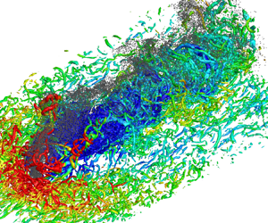

1. Introduction
Transverse jets are formed when jets are injected perpendicularly to cross-flows, which are widely encountered in various scenarios such as combustion chambers in gas turbines and scramjet engines. There are complex interactions between the jet and cross-flow, which can improve the mixing of the two streams. The fundamental structure of transverse jets is depicted in figure 1. As can be seen, the jet is deflected in the direction of the cross-flow. In the near-field of the jet exit, lateral shearing gives rise to shear layer vortices, which evolve into counter-rotating vortex pair (CVP) structures in the far-field (Muppidi & Mahesh Reference Muppidi and Mahesh2007). The CVP structures possess the highest vorticity in transverse jets, contributing to the enhancement of mixing (Karagozian Reference Karagozian2010). Around the windward side of the jet, flow separation occurs due to negative pressure gradients imposed by the jet, forming streamwise horseshoe vortices that propagate downstream along the periphery of the jet. In the downstream region, flow separation within the boundary layer gives rise to upright trailing vortices penetrating both the incoming flow boundary layer and the leeward side of the jet (Fric & Roshko Reference Fric and Roshko1994).
The main structure of a low-speed transverse jet (Karagozian Reference Karagozian2010).

In scramjet engines, enhanced mixing of the fuel and air is desirable due to the short residence time of the flow, which can be achieved with high-speed transverse jets. In comparison with low-speed transverse jets, the compressible effect of the fluid significantly influences the flow characteristics of high-speed transverse jets. The typical structure of a high-speed jet in supersonic cross-flow (JISC) is illustrated in figure 2. As the jet interacts with the cross-flow, a bow shock is generated in the upstream region. The boundary layer of the incoming cross-flow undergoes flow separation due to the negative pressure gradient around the jet, forming horseshoe vortices propagating downstream around the jet. As being injected, the jet fluid experiences an expansion followed by compression induced by the barrel shock and Mach disc. The Mach disc structure is highly unstable, leading to the formation of strong shear flows and significant large-scale quasi-coherent vortex structures downstream. The core region of the jet experiences lateral shearing from the incoming flow, generating large-scale CVP structures, which are similar to those observed in the low-speed counterparts. Recirculation zones are observed in the upstream and downstream regions around the jet exit due to negative pressure gradients. The downstream recirculation zone induces the formation of CVPs in the near-wall region.
A schematic of the time-averaged structure of a compressible JISC (Dickmann & Lu Reference Dickmann and Lu2009).

Due to their practical importance, compressible transverse jets have been extensively studied experimentally. Gruber et al. (Reference Gruber, Nejad, Chen and Dutton1995, Reference Gruber, Nejad, Chen and Dutton1997a,Reference Gruber, Nejad, Chen and Duttonb, Reference Gruber, Nejad, Chen and Dutton2000) conducted a series of experiments of sonic jets transversely injected into a Mach 1.98 cross-flow. It was found that, with a constant jet-to-cross-flow momentum ratio, increasing the compressibility of the jet enhances the convective velocity of large-scale vortical structures in the near-field. Compressible effects exhibit minimal effect on the penetration of the jet in the vertical and streamwise directions but suppress the turbulence intensity within the transverse jet shear layer. Santiago & Dutton (Reference Santiago and Dutton1997) conducted quantitative measurements on compressible sonic transverse jets injected into a Mach 1.6 cross-flow. The results showed that within the leeward region of the barrel shock, the Reynolds stress of the fluid is minimal. VanLerberghe et al. (Reference VanLerberghe, Santiago, Dutton and Lucht2000) used laser-induced fluorescence to investigate the momentum exchange between the cross-flow and jet, and found that the most intensive mixing region exists in the wake region of the barrel shock, just beneath the centreline of the jet. The fluid of the jet traverses from the upper edge of the bow shock across the Mach disc, penetrating deeply downstream, which plays a significant role in generating large-scale turbulent structures within the shear layer above the jet centreline.
With the development of computers and modelling techniques, numerical simulations have been employed for JISC. Kawai & Lele (Reference Kawai and Lele2010) compared the flow structures and statistical characteristics of a sonic jet injected into a Mach 1.6 cross-flow under laminar and turbulent conditions using large-eddy simulation (LES). The results show that the regions with high turbulent kinetic energy (TKE) correspond to vortex-generating zones, where the concentration of the jet fluid is notably low, indicating a significant enhancement in turbulent diffusion of the jet fluid. By comparing the results of the laminar and turbulent cases with the experimental data, it was found that the turbulent case better captures the structure of the bow shock and exhibits better agreements with the experimental data. Chai, Iyer & Mahesh (Reference Chai, Iyer and Mahesh2015) employed LES to model two cases: one is featured by a sonic jet injected into a Mach 1.6 cross-flow and the other by a Mach 3.73 jet injected into a Mach 0.8 cross-flow. The study compared the results of the cases with laminar and turbulent cross-flows. Génin & Menon (Reference Génin and Menon2010) utilised LES to simulate sonic transverse jets injected into cross-flows with Mach numbers of 1.6 and 2.0. The study focused on the Kelvin–Helmholtz (KH) instability and revealed that the upstream horseshoe vortices result from the interactions between the incoming boundary layer structure and the jet near the wall. Rana, Thornber & Drikakis (Reference Rana, Thornber and Drikakis2011) conducted LES to explore the interaction between a sonic jet and a Mach 1.6 cross-flow. It was shown that the KH instability occurs within the shear layer upstream of the jet, which evolves into large-scale vortical structures that propagate downstream with an efficient and rapid mixing process.
Direct numerical simulation (DNS) represents a powerful tool for understanding the fundamentals of turbulent flows, which has been used for high-speed transverse jet flows in recent years. Sun & Hu (Reference Sun and Hu2018a,Reference Sun and Hub,Reference Sun and Huc) and Sun, Liu & Hu (Reference Sun, Liu and Hu2019) have made significant progress in DNS of high-speed transverse jet flows. The authors mainly focused on the compressible turbulent boundary layer inflow with a Mach number of 2.7 and various momentum ratios of 1.85, 2.3 and 5.5 for sonic jets. It was found that the bow shock near the wall diminishes the turbulence intensity of downstream flow significantly, and this attenuation increases with higher momentum ratio values. Flow separation near the jet exit and lateral expansion downstream cause a reduction in turbulence intensity near the wall and disrupt coherent structures, thus resulting in the laminarisation in the boundary layer. However, it gradually transitions back to a turbulent state as propagating further downstream. An increase in the momentum ratio prolongs the time required for this return. IN addition, extensive studies have been conducted on the large-scale CVP structures. The CVP structures dominate the mixing in the near-field and fracture into smaller vortex structures in the far-field, thus intensifying the flow mixing in the far-field. Above the primary CVP structure, there exists an attached pair of smaller CVP structures, formed in relation to the Mach disc. As streamlines traverse both sides of the Mach disc, oblique pressure moments induce strong shearing forces, resulting in the formation of attached CVP structures rotating in the opposite direction to the primary CVP structure.
Solid-fuelled scramjet is a supersonic ramjet employing a solid fuel, which has the advantages of simple fuel supply and compactness. In solid-fuelled scramjets, particle-laden jets are injected into supersonic cross-flows. A few studies of gas–solid two-phase transverse jets have been carried out in the context of Eulerian–Lagrangian framework, most of which focused on subsonic or low-Mach-number conditions. Campolo, Salvetti & Soldati (Reference Campolo, Salvetti and Soldati2005) used a one-way coupling model to simulate the interaction between a transverse jet loaded with a large number of point-source particles and the cross-flow. It was found that small particles, due to their lower inertia, are influenced significantly by the vortical structures around the jet, predominantly accumulating on the lee side of the jet. In contrast, larger particles, owing to their greater inertia, could penetrate to deeper heights along the jet trajectory, with less-significant selective clustering. Salewski & Fuchs (Reference Salewski and Fuchs2008) conducted simulations using four-way coupling with LES to investigate the interaction between a transverse jet with a high particle loading and a subsonic cross-flow. The simulations showed that four-way coupling reduces the forces experienced by particles near the jet exit significantly, particularly close to the wall. Moreover, the four-way coupling facilitate larger penetration of the particles. Li & Lin (Reference Li and Lin2010) utilised the Reynolds-averaged Navier–Stokes (RANS) method to simulate the interaction between a two-way coupled particle-laden transverse jet and a subsonic cross-flow with a jet momentum ratio of  $J=11$. The simulations highlighted a significant disparity between the jet trajectory based on the particle concentration field within the near-field and the jet trajectory defined using gas-phase mean velocities, particularly when the Stokes number of the particles was high. The CVP structures and wake vortices predominantly influence particle dispersion downstream, resulting in the primary particle accumulation on the lee-side of the jet trajectory. In addition, at higher particle Stokes numbers, the CVP structures are also modulated by the particles.
It is noted that compressible gas–solid two-phase transverse jets interacting with supersonic cross-flows have not yet been studied using DNS. The modulation mechanisms of particles on the turbulence and shock wave structures in JISC, as well as the distribution and dynamics of particles in compressible transverse jets, remain unknown. Conducting in-depth and systematic investigations on this issue would contribute to a deeper understanding of compressible gas–solid two-phase transverse jets. Therefore, the main objective of the present study is to carry out the first DNS of compressible gas–solid two-phase transverse jets, aiming at revealing the characteristics of particle distribution and the influence of particles on the flow field.
This paper is organised as follows. Section 2 details the simulation set-ups, including grid system, boundary conditions and various parameters of the simulations. In § 3, the descriptions of governing equations for the fluid phase, Lagrangian particle-tracking methods and numerical algorithms are provided. The results of single-phase JISC, jet and particle trajectories, particle dispersion, modulation of particles on turbulence and shocks are discussed in § 4. The conclusions are presented in § 5.
2. DNS configuration and numerical details
The DNS configuration of sonic transverse jets injected into supersonic cross-flows is considered in the present work. We chose the condition with a flying height at 25 km above the ground, where the ambient temperature is 222 K and the ambient pressure is 2.5 kPa. The flying Mach number is 7.2. The resultant Mach number of the cross-flow is  $Ma=2$, which represents the flow conditions in a combustion chamber of a hypersonic vehicle (Paull, Stalker & Mee Reference Paull, Stalker and Mee1995; Urzay Reference Urzay2018). The speed, density and temperature of the cross-flow are
 $u_0=1.0$,
 $\rho _0=1.0$ and
 $T_0=1.0$, respectively, while those of the jet are
 $v_{jet}=0.6126$,
 $\rho _{jet}=7.84$ and
 $T_{jet}=1.5$, respectively. The diameter of the jet exit is
 $D = 36$. The momentum ratio of the jet and cross-flow is
 $J=(\rho _{jet}v_{jet}^2)/(\rho _0u_0^2)=2.9$. The Reynolds number is
 $Re=\rho _0u_0\theta _{in}/\mu _0=180$, where
 $\mu _0$ is the dynamic viscosity of the cross-flow and
 $\theta _{in}$ is the inflow momentum thickness. Note that the variables in the present work are in a non-dimensional form. The reference values used for normalisation are provided in table 1.
Reference values for normalisation.

The isothermal no-slip condition is used at the wall (Poinsot & Lelef Reference Poinsot and Lelef1992). Non-reflecting Navier–Stokes characteristic boundary conditions are imposed at the upper boundary, streamwise outlet and both spanwise outlets. The inflow is featured by a fully developed compressible turbulent boundary layer extracted from a precursor DNS, which can efficiently produce a high-fidelity compressible turbulent boundary layer, and is suitable to serve as the incoming supersonic cross-flow for the present configuration. The friction Reynolds number of the compressible turbulent boundary layer at the inlet is  $Re_{\tau } = 321$. For more details and validations of the precursor DNS, please refer to our previous work (Xiao et al. Reference Xiao, Jin, Luo, Dai and Fan2020).
The domain size is  $Lx\times Ly\times Lz=2716\times 632\times 720$ in the streamwise, wall-normal and spanwise directions, respectively. Take the centre of the jet exit as the origin of the coordinate system, the computational domain can be denoted as
 $Lx\approx [-35D,40D]$,
 $Ly\approx [0,17.5D]$ and
 $Lz\approx [-10D,10D]$. This domain is large enough for the evolution and propagation of the upstream compressible turbulent boundary layer and downstream transverse jet structures.
Due to the presence of near-wall turbulence and shock structures surrounding the transverse jet, we introduce a clustered grid system based on our previous work of a compressible turbulent boundary layer (Xiao et al. Reference Xiao, Jin, Luo, Dai and Fan2020). A schematic of the grid size distribution in the streamwise direction is given in figure 3(a). The resolution of  $\Delta x=2.85$ was proved to be fine enough in characterising the boundary layer turbulence in our previous study (Xiao et al. Reference Xiao, Jin, Luo, Dai and Fan2020), which is further refined in the JISC region to capture the complex shock and turbulence structures. The grids in the wall-normal direction are also consistent with our previous work (Xiao et al. Reference Xiao, Jin, Luo, Dai and Fan2020). There are 310 grid points within the height of
 $Ly=632$, and the grids are stretched based on a hyperbolic-tangent function. Note that uniform grids with
 $\Delta y=0.5136$ are used within
 $y=18.07\sim 49.91$ to better resolve the bow shock, barrel shock and turbulence structures, as shown in figure 3(b). In the spanwise direction, the grids are uniform with a resolution of
 $\Delta z=1.45$ in the core region of
 $|z|\le 5.5D$. Out of this region, grids are stretched smoothly to damp fluctuations and minimise reflections of physical waves in the spanwise direction. This mesh resolution is fine enough to capture small-scale turbulence in the near-wall region and the large-scale structures of compressible turbulent boundary layer (Poggie, Bisek & Gosse Reference Poggie, Bisek and Gosse2015). The resultant grid number is
 $Nx\times Ny\times Nz=1260\times 310\times 414$. A sensitivity study of the resolution has not been performed in the present work as the computational cost would not be affordable.
The distributions of grid size in the (a) streamwise and (b) wall-normal directions.

Particles are released at the jet exit with a particle mass loading of  $\varPhi _{m,jet} = 0.1$, which is expressed as follows:
 \begin{equation} \varPhi_{m,jet}=\frac{\rho_pN_{p,jet}V_p}{\rho_{jet}v_{jet}A_{jet}\Delta t}, \end{equation}
where  $N_{p,jet}$ is the number of particles injected per time step,
 $\rho _p$ is the particle density,
 $V_p$ is the volume of particles,
 $\Delta t$ is the time step and
 $A_{jet}$ is the area of the jet exit.
Two cases with different particle diameters are considered in the present work. Table 2 provides various parameters of the particles for the two cases, including the particle Stokes number  $St$, particle density
 $\rho _p$, particle diameter
 $d_p$, ratio of the particle diameter
 $d_p$ to minimum Kolmogorov length scale
 $\eta _{min}$, particle relaxation time
 $\tau _p$, inflow particle volume fraction
 $\varPhi _{v,jet}$ and particle number in the domain
 $N_p$. The particle Stokes number
 $St={\tau _p}/{\tau _f}$ is based on the particle relaxation time
 $\tau _p=\rho _pd_p^2/(18\mu )$ and characteristic flow time
 $\tau _f={D}/{v_{jet}}$. In both cases, the particle diameters are smaller than the smallest Kolmogorov length scale. In this work, we are interested in the preferential concentration of particles, in which the Stokes number plays an important role (Balachandar & Eaton Reference Balachandar and Eaton2010). In particular, preferential concentration is most important when the Stokes number is close to unity, while particles with very small Stokes number can follow the fluid motion. Therefore, the particle diameters in the present work are determined so that the Stokes numbers of cases A and B are 1.0 and 0.1, respectively. The inflow particle volume fraction is
 $\varPhi _{v,jet}=5.23\times 10^{-4}$, which is suitable for the employment of two-way coupling strategy (Balachandar & Eaton Reference Balachandar and Eaton2010). The dimensional particle diameters are 640 and 200 nm for cases A and B, respectively. We note that the sizes of selected particles are in the range of particle fuels for applications such as gas turbines and internal combustion engines (Bergthorson Reference Bergthorson2018). Moreover, transmission electron microscopy (TEM) images have shown that the nanopowders used in engines consists of mostly spherical particles (Mandilas et al. Reference Mandilas, Karagiannakis, Konstandopoulos, Beatrice, Lazzaro, Di Blasio, Molina, Pastor and Gil2014). Since the particle mass loading is identical in the two cases, the number of large particles is much less than that of small particles.
Particle parameters for the two cases.

The statistics of the flow and particles are collected in a time period of  ${100D}/{u_0}$ after reaching the statistically steady state. The averages are carried out at each grid point unless being specifically declared. Statistical data of Lagrangian particles are averaged over all particles nearest to a local Eulerian grid to provide the mapping of Lagrangian data to the Eulerian system.
3. Numerical methods
3.1. Governing equations for the fluid phase
In the present work, the carrier phase is assumed to be a compressible Newtonian fluid, which is solved with the compressible Navier–Stokes equations in a conservative and non-dimensional form:
 $$\begin{gather} \frac{\partial\rho}{\partial t}+\frac{\partial(\rho u_j)}{\partial x_j}=0, \end{gather}$$
 $$\begin{gather}\frac{\partial(\rho u_i)}{\partial t}+\frac{\partial}{\partial x_j}\left(\rho u_iu_j+p_m\delta_{ij}-\frac{1}{Re}\sigma_{ij}\right)=\varphi_{ui}, \end{gather}$$
 $$\begin{gather}\frac{\partial E}{\partial t}+\frac{\partial}{\partial x_j}\left((E+p_m)u_j-\frac{1}{Re}u_i\sigma_{ij}- \frac{1}{PrRe(\gamma-1)Ma^2}\left(k\frac{\partial T}{\partial x_j}\right)\right)=\varphi_E, \end{gather}$$
where  $\rho$ and
 $u_j$ are the density and velocity, respectively. Here,
 $p_m={p}/{(\gamma M a^2)}$ denotes the normalised pressure,
 $\delta _{ij}$ is the Kronecker delta,
 $T$ is the temperature,
 $Pr$ is the Prandtl number and
 $E$ is the total energy per unit volume and is defined as
 \begin{equation} E=\frac{1}{2}\rho u_iu_i+\frac{p_m}{\gamma-1}, \end{equation}
where  $\gamma =1.4$ is the heat capacity ratio. The viscous stress tensor
 $\sigma _{ij}$ is given as
 \begin{equation} \sigma_{ij}=\mu\left(\frac{\partial u_i}{\partial x_j}+\frac{\partial u_j}{\partial x_i}-\frac{2}{3}\frac{\partial u_i}{\partial x_i}\delta_{ij}\right), \end{equation}
where  $\mu$ is the dynamic viscosity and
 $k$ is the thermal conductivity, both of which follow the Sutherland law (Sutherland Reference Sutherland1893):
 \begin{equation} \mu=k=\frac{1.4041T^{3/2}}{T+0.40417}. \end{equation}
The two-way coupling approach is adopted for the gas–solid two-phase JISC. The right-hand-side terms in the momentum and energy governing equations represent the feedback force and heat terms, respectively, which are calculated as
 $$\begin{gather} \varphi_{ui}={-}\sum_{i=1}^{N}{\frac{m_p}{V_m}F_iS(i)}, \end{gather}$$
 $$\begin{gather}\varphi_E={-}\sum_{i=1}^{N}{\frac{m_p}{V_m}F_iv_{p,i}S(i)}, \end{gather}$$
where  $N$ is the particle number in a given control volume
 $V_m$,
 $m_p$ is the mass of a single particle and
 $F_i$,
 $v_i$ and
 $S(i)$ are the drag force, velocity and trilinear interpolation coefficient of the
 $i$th particle, respectively (Sundaram & Collins Reference Sundaram and Collins1999). These feedback force and heat are exerted to the nearest eight surrounding fluid nodes to ensure the momentum and energy conservation. The descriptions of particle equations are provided in the following.
3.2. Lagrangian particle tracking
The particle density is very high compared with the fluid density, and the particle diameter is very small. Therefore, the point-particle method is used to track the particles in a Lagrangian way without considering the volume effect. Only the Stokes drag force term is important and considered in the particle equations (Ling, Parmar & Balachandar Reference Ling, Parmar and Balachandar2013). Other force terms, including the shear and rotation lift forces, gravitational force, buoyancy force and pressure gradient force, are neglected. The particle slip Mach number is relatively low for most particles; therefore, the correction related to the compressibility effect on the drag force coefficient is also ignored (Loth Reference Loth2008). Moreover, the particle volume fraction in the whole computational domain is rather low, therefore the particle–particle collision is ignored for simplicity (Hadinoto et al. Reference Hadinoto, Jones, Yurteri and Curtis2005).
Based on the above discussions, the Basset–Boussinesq–Oseen equations (Parmar, Haselbacher & Balachandar Reference Parmar, Haselbacher and Balachandar2011, Reference Parmar, Haselbacher and Balachandar2012) are applied to track the particles, which can be expressed as
 $$\begin{gather} \frac{{\rm d}\kern0.7pt x_{p,i}}{{\rm d} t}=v_{p,i}, \end{gather}$$
 $$\begin{gather}\frac{{\rm d} v_{p,i}}{{\rm d} t}=\frac{F_{p,i}}{m_p}=\frac{f}{\tau_{p,i}}(u_{p,i}-v_{p,i}), \end{gather}$$
where  $x_{p,i}$ is the
 $i$th particle position and
 $u_{p,i}$ is the fluid velocity at the
 $i$th particle position. In the present work, the point-particle method was employed. As the grid size is much larger than the particle size, the unperturbed fluid properties at the particle position can be approximated by the interpolated values at the position of a specific particle. We note that this method has been widely used in previous studies of two-way coupling simulation (Ferrante & Elghobashi Reference Ferrante and Elghobashi2003; Gualtieri et al. Reference Gualtieri, Picano, Sardina and Casciola2013). The particle mass is given as
 $m_p={\pi d_p^3\rho _p}/{6}$. Here
 $F_{p,i}$ is the force applied to the particles by fluid and
 $f=1+0.15{Re}_p^{0.687}$ is the correction for the particle drag force (Schiller & Naumann Reference Schiller and Naumann1933), where
 ${Re}_p$ is the slip Reynolds number of the particle. The probability density functions (PDFs) of the particle Reynolds number are shown in figure 4(a). As can be seen, the particle Reynolds numbers are lower than 20 for both cases, so that using the Schiller and Naumann correction (Schiller & Naumann Reference Schiller and Naumann1933) for the drag coefficient is suitable. According to (Loth Reference Loth2008), the effects of compressibility and rarefaction on particle drag could be neglected when
 $Ma_p < 0.4$, where
 $Ma_p$ is the particle Mach number. As can be seen from figure 4(b), most particles have a particle Mach number lower than 0.4. Therefore, the effects of compressibility and rarefaction can be neglected. Note that the gravity is neglected in (3.9) as the drag force is much larger than the force applied to the particles by gravity. The particle-wall bouncing model is assumed to be fully elastic.
The PDFs of (a) particle Reynolds number and (b) particle Mach number for various cases.

3.3. Numerical schemes
For the fluid phase, a hybrid weighted essentially non-oscillation (WENO) scheme is applied to discretise the convective terms. Due to the presence of large-scale bow-shock structure in the JISC, extreme high dissipation and high discontinuity exist simultaneously in the flow field. Therefore, a local sensor is applied to detect the dissipation  $\varTheta$ and classify the flow field as high-dissipation regions and high-discontinuity regions (Pirozzoli & Bernardini Reference Pirozzoli and Bernardini2011), as given below:
 \begin{equation} \varTheta=\frac{(\boldsymbol{\nabla}\boldsymbol{\cdot} u)^2}{(\boldsymbol{\nabla}\boldsymbol{\cdot} u)^2+ (\boldsymbol{\nabla}\times u)^2+\left(\dfrac{u_0}{\delta_{in}}\right)^2}. \end{equation}
In the high-discontinuity region with  $\varTheta \geq 0.01$, a seventh-order WENO-JS (Shu Reference Shu2020) is applied to damp the discontinuity and enhance numerical stability. In the other more dissipative regions, an eighth-order accurate bandwidth-optimised weighted essentially non-oscillation (WENO-BO4) scheme (Martín et al. Reference Martín, Taylor, Wu and Weirs2006) is adopted to capture discontinuity well. To further reduce the dissipation of the WENO-BO4 scheme when resolving turbulence structure in the continuous region, a total variation-based relative limiter (Duan, Choudhari & Wu Reference Duan, Choudhari and Wu2014; Duan, Choudhari & Zhang Reference Duan, Choudhari and Zhang2016) is added to the WENO-BO4 scheme. An eighth-order standard central difference scheme is used for diffusion terms, and a third-order total variation diminishing (TVD) Runge–Kutta multistage method (Shu & Osher Reference Shu and Osher1988) for time advancement.
Regarding the dispersed phase, the third-order TVD Runge–Kutta method is employed for time advancing of particle positions and velocities. Since the particles and fluid are tracked in different frameworks, interpolation and mapping between the Eulerian system and the Lagrangian system are required. All variables of the fluid parameters at the particle position are interpolated using a trilinear scheme from the values of the surrounding eight grid points. In a similar way, the Lagrangian particle forces and heat on the fluid phase are mapped on the nearest eight Euler grid-points by the same trilinear scheme. Note that we have post-processed the fluid velocity data of at the particle position using different interpolation schemes. In particular, the trilinear interpolation and the cubic spline interpolation were tested. The statistical results based on the two interpolation schemes are almost the same. Therefore, the choice of trilinear interpolation is justified. The trilinear interpolation has also been widely used in the simulations of multiphase flows with the point-particle method (Gualtieri et al. Reference Gualtieri, Picano, Sardina and Casciola2013; Dai et al. Reference Dai, Luo, Jin and Fan2017; Mehrabadi et al. Reference Mehrabadi, Horwitz, Subramaniam and Mani2018).
The numerical methods in the present study have been validated in our previous studies on various types of compressible turbulent flows, including the interaction of detonation and isotropic turbulence (Jin et al. Reference Jin, Luo, Dai and Fan2016b), compressible jet flows (Luo et al. Reference Luo, Jin, Lu and Fan2013; Jin et al. Reference Jin, Luo, Dai and Fan2016a), compressible HIT (Dai et al. Reference Dai, Luo, Jin and Fan2017), compressible mixing layers and compressible turbulent boundary layer flows (Xiao et al. Reference Xiao, Jin, Luo, Dai and Fan2020).
4. Results and discussion
4.1. The characteristics of single-phase JISC
The structures of single-phase JISC are first presented. The instantaneous distributions of the density gradient magnitude at the central  $x$–
 $y$ plane and the streamwise velocity at a wall-normal plane with
 ${y}/{D}\approx 0$ are shown in figure 5, where the mean flow direction is from left to right. As can be seen, a bow shock exists ahead of transverse jet. The jet serves as an obstacle and induces an adverse pressure gradient to trigger the separation of the inflow turbulent boundary layer to form a recirculation zone in front of the jet. This recirculating flow further results in compression waves, which forms a
 $\lambda$ shape structure together with the bow shock. The jet fluids rapidly expand in radial directions after leaving the jet exit, and form the windward barrel shock, leeward barrel shock and Mach disc structure under the influence of the supersonic cross-flow. In the far-field, large-scale shear layer structures is generated, with a reflecting wave above it. As the flow further propagates downstream, the influence of the transverse jet on the near-wall turbulence is reduced, and the typical structures of boundary layer turbulence gradually recover.
The instantaneous structures of the sonic transverse jet injected to the Mach 2 supersonic turbulent cross-flow (propagated from left to right). Contours of density gradient magnitude at the central  $x$–
 $y$ plane and of instantaneous streamwise velocity near the wall are shown in a three-dimensional view together.

Figure 6 shows the instantaneous isosurfaces of the second invariant of the velocity gradient tensor, i.e. the  $Q$-criterion, coloured by the fluid density, which is calculated as follows (Hunt, Wray & Moin Reference Hunt, Wray and Moin1988):
 \begin{equation} Q=\frac{1}{2}\left(\theta^2-s_{ij}s_{ji}+\frac{\omega_k\omega_k}{2}\right)= \frac{1}{2}\left(\left(\frac{\partial u_i}{\partial x_i}\right)^2- \frac{\partial u_i}{\partial x_j}\frac{\partial u_j}{\partial x_i}\right), \end{equation}
where  $\theta ={\partial u_i}/{\partial x_i}$ is the velocity divergence,
 $s_{ij}={({\partial u_i}/{\partial x_j}+{\partial u_j}/{\partial x_i})}/{2}$ is the strain rate tensor component and
 $\omega _k$ is the vorticity component. It can be seen that the flow is highly three-dimensional and consists of coherent vortical structures with various scales. A large number of large-scale horseshoe vortices are observed surrounding the jet exit, which propagate downstream and interact with the transverse jet in the far field. In the near-wall region immediately downstream of the jet exit, hairpin vortices are induced, while in the lateral side of the jet exit, the near-wall coherent vortex structures are largely damped due to the presence of the bow-shock structure.
The three-dimensional visualisation of  $Q$-vortex structures, coloured by the local fluid density.

To identify the influence of the transverse jet on the turbulent boundary layer structure, figure 7 shows the contours of instantaneous density at a wall-normal plane near the wall with  ${y}/{D}=0.08$. The typical streak structures with varying densities are observed in the upstream region of the jet. However, the transverse jet severely damps the streak structures, enhances the local fluid densities and weakens the density fluctuations. As the streamwise distance increases, i.e.
 ${x}/{D}\geq 10$, the near-wall streak structures gradually recover.
Contours of instantaneous density on a wall-normal plane at  ${y}/{D}=0.08$.

The mean flow structures are also analysed. Figure 8 shows the distributions of the mean Mach number, mean streamwise velocity, TKE and Reynolds stress in the central  $x$–
 $y$ plane. The mean Mach number contour clearly shows the bow shock, barrel shock and Mach disc structures. The regions with negative mean streamwise velocities near the wall indicate the existence of upstream and downstream recirculation zones. As shown in figures 8(c) and 8(d), significant velocity gradients at the shock front result in large values of TKE and Reynolds stress, which reach a local maximum downstream of the barrel shock structures, corresponding to the formation of CVP structures. The CVP structures are examined in figure 9 in terms of the mean streamwise vorticity at the
 $y$–
 $z$ plane with
 ${x}/{D}=3$, where one major and two minor vortex pairs exist. These complex CVP structures agree well with previous studies (Sun & Hu Reference Sun and Hu2018a).
Contours of time-averaged (a) Mach number  $Ma$, (b) streamwise velocity
 $\bar {u}$, (c) TKE and (d) Reynolds stress
 $\overline {u^\prime v^\prime }$ at the central
 $x$–
 $y$ plane.

Contour of time-averaged streamwise vorticity  $\overline {\omega _x}$ on the
 $y$–
 $z$ plane with
 ${x}/{D}=3$.

4.2. Trajectories of the jet and particles
In the study of JISC, the jet trajectories are of great importance in characterising the jet penetration and the mixing between the jet and cross-flow, which have been investigated extensively. There are various ways in defining the jet trajectories, such as based on the local maximum of fluid velocity (Kamotani & Greber Reference Kamotani and Greber1972; Beresh et al. Reference Beresh, Henfling, Erven and Spillers2005) or local maximum of scalar concentration (Gruber et al. Reference Gruber, Nejad, Chen and Dutton1997a; Smith & Mungal Reference Smith and Mungal1998; Ben-Yakar, Mungal & Hanson Reference Ben-Yakar, Mungal and Hanson2006). However, the determination of the local maximum in the unsteady three-dimensional flow is not unique and may lead to numerical uncertainties (Yuan & Street Reference Yuan and Street1998). Therefore, the mean streamline originating from the centre of the jet exit is considered as the jet trajectory in the present work. The mean streamline-based jet trajectory has been widely used in previous studies (Muppidi & Mahesh Reference Muppidi and Mahesh2005; Chai et al. Reference Chai, Iyer and Mahesh2015; Sun & Hu Reference Sun and Hu2018a). In addition to the jet trajectory, the mean trajectory of the particles is also studied, which is defined as the trajectory of the centre of mean particle concentration and is referred to as the mean concentration-based particle trajectory in the following.
Figure 10 shows the mean streamline-based jet trajectories of various DNS cases. It has been shown that the jet penetration into the cross-flow is mainly controlled by the momentum ratio of the jet and cross-flow, i.e.  $J$. Many experimental data have been used to derive the correlations for jet trajectory in the literature, which are based on a power law or a logarithmic fit (Vranos & Nolan Reference Vranos and Nolan1965; Rothstein & Wantuck Reference Rothstein and Wantuck1992; Gruber et al. Reference Gruber, Nejad, Chen and Dutton1997a). In particular, the correlation proposed by Vranos & Nolan (Reference Vranos and Nolan1965) is expressed as
 \begin{equation} \frac{y}{D}=1.68J^{0.5}(x/D)^{0.0866}. \end{equation}
The correlation of Rothstein & Wantuck (Reference Rothstein and Wantuck1992) with a logarithmic fit is written as
 \begin{equation} \frac{y}{D}=J^{0.312}\ln[4.704(x/D+0.637)]. \end{equation}
Based on planar Rayleigh/Mie scattering measurements of sonic jets injecting into supersonic cross-flow, Gruber et al. (Reference Gruber, Nejad, Chen and Dutton1997a) proposed the following correlation using a power law curve fit:
 \begin{equation} \frac{y}{DJ}=1.20[(x+D/2)/DJ]^{0.344}. \end{equation}
The mean streamline-based jet trajectories are compared with the predictions based on the above-mentioned correlations. As can be seen, the jet trajectories of various cases are within the range of predictions by different correlations. Better agreement is achieved between the DNS result and the correlation by Vranos & Nolan (Reference Vranos and Nolan1965).
The mean streamline-based jet trajectories (solid lines) and mean concentration-based particle trajectories (dotted lines) of various cases. The predictions based on various correlations (Vranos & Nolan Reference Vranos and Nolan1965; Rothstein & Wantuck Reference Rothstein and Wantuck1992; Gruber et al. Reference Gruber, Nejad, Chen and Dutton1997a) for the jet trajectories are also shown (dashed lines).

The mean concentration-based particle trajectories are also presented in figure 10. It can be seen that large particles travel evidently higher than small particles. As the jet evolves, the trajectories of large particles and small particles gradually coincide, at a higher position than the jet trajectory. This indicates that the particle distributions are affected by the shear layer in the windward side of the transverse jet structure, as is further explored in the next section.
4.3. Particle dispersion
In this section, we compare the behaviours of particle dispersion in the two particle-laden cases. Figure 11 displays the instantaneous distribution of  $Q$-vortex and particles in case A. The particles are represented by grey points. The vortical structures are coloured by the local fluid density. As can be seen, the particles near the jet exit are subjected to radial expansion. Nevertheless, the particles at the centre of the jet exit follow the jet trajectory, and are further entrained into the windward side shear layer in the downstream regions. Most large particles disperse around the jet rather than in the boundary layer. In contrast, small particles can be transported into the boundary layer structures, which is detailed later.
Instantaneous snapshot of the isosurface of  $Q$-vortex structures and large particles of two-phase JISC in case A. Particles are indicated by grey points.

To investigate the particle dispersion characteristics in the JISC, we present the instantaneous distributions of particles in typical planes. Figure 12 shows the particle dispersion in the central  $x$–
 $y$ plane for case A. It can be seen from figure 12(a) that the particles slightly spread in the radial direction after being injected from the jet exit. It is interesting to observe that large particles are mainly transported to the windward shear layer of the transverse jet above the boundary layer structures. In the far-field, as shown in figure 12(b), the flow exhibits significant density stratification, i.e. the fluid density in the boundary layer is much lower compared with that after the bow shock. Due to the recovery of the boundary layer structures, some large particles in the downstream regions are swept towards the near-wall regions, whereas many particles remain in the outer regions because of their large inertia.
Instantaneous snapshots of the flow fields and large particles at the central  $x$–
 $y$ plane
 ${z}/{D}=0$ in case A: (a) near-field contour of streamwise velocity; (b) far-field contour of fluid density.

Figure 13 shows the particle dispersion in the central  $x$–
 $y$ plane for case B. It is evident that the distribution of small particles is quite different from that of large particles. In particular, small particles can travel further in the radial direction after injection due to smaller inertia. This results in the existence of particles in the front and back recirculation zones, as indicated by the red circles. Therefore, small particles spread widely in the near-wall regions and in the boundary layer. Moreover, small particles in the windward side of the jet trajectory propagate downstream with the evolution of the large-scale shear layer structure, as shown in figure 13(a). In the far-field, small particles are driven by the shedding vortices in the outer layer of the boundary layer and accumulate in the high-density regions due to the centrifugal effect, which can be clearly seen in the figure 13(b).
Instantaneous snapshots of the flow fields and large particles at the central  $x$–
 $y$ plane
 ${z}/{D}=0$ in case B: (a) near-field contour of streamwise velocity; (b) far-field contour of fluid density.

To further explain the behaviour of radial expansion in the near-field, the mean radial velocity profiles of fluid and particles for various cases at  $y/D = 1$ are shown in figure 14. The radial velocity represents the velocity component in the radial direction and the radial distance is calculated as
 $r=\sqrt {x^2+z^2}$. As can be seen, the mean radial velocity of fluid is positive and increases with increasing radial distance, confirming the lateral expansion of the fluid. The profiles of mean fluid radial velocity for the two cases almost overlap when
 $r/D< 0.65$. For both cases, the mean radial velocity of particles is lower than that of fluid. Moreover, the mean radial velocity of particles in case B is larger than that in case A. This is because smaller particles have lower inertia, which tend to follow the fluid more closely, thus smaller particles travel further in the radial direction after injection.
The mean radial velocity profiles of fluid and particles for various cases at  $y/D = 1$.

The particle distributions in typical  $y$–
 $z$ planes with
 ${x}/{D}=3$ and
 $35$ for case A are shown in figures 15 and 16, respectively. It can be seen from figure 15 that large particles mainly accumulate above the main CVP. As the particles move downstream, most of them still distribute in the low-density regions around the jet wakes, while a few are transported towards the near-wall regions and lateral sides, as shown in figure 16. Evident preferential concentration of particles, which is due to the complex interactions of particles and vortices, is observed in the downstream region, which are examined in detail later.
Instantaneous snapshots of the flow fields and large particles at the  $y$–
 $z$ plane with
 ${x}/{D}=3$ in case A: (a) fluid density; (b) streamwise vorticity.

Instantaneous snapshots of the flow fields and large particles at the  $y$–
 $z$ plane with
 ${x}/{D}=35$ in case A: (a) fluid density; (b) streamwise vorticity.

In contrast to large particles, small particles in the near-field do not only appear above the main CVP, but also exist in the bilateral sides of the near-wall wake regions immediately downstream the jet exit, as shown in figure 17. It is observed that in the upstream region ( $x/D = 3$) large particles are concentrated above the CVP while small particles can also exist around the CVP. This is not just due to the centrifugal force of the vortex. After being ejected from the jet exit, the radial expansion of large particles is relatively limited. They mainly follow the trajectory of the jet and arrive above the CVP. This corresponds to the windward side of the shear layer. In addition to this mechanism, small particles experience more significant radial expansion and then follow the fluid until the vicinity of the Mach disc. Here, the particles, after experiencing intense shear action, are flung to the lateral sides of the low-vorticity region around the CVP. Under the influence of the streamwise vortices, small particles are transported downstream and diffuse into the whole boundary layer. This results in the wide spread of small particles both in the low-density regions in the outer jet wake and in the near-wall boundary layer regions in the far-field as shown in figure 18.
Instantaneous snapshots of the flow fields and small particles at the  $y$–
 $z$ plane with
 ${x}/{D}=3$ in case B: (a) fluid density; (b) streamwise vorticity.

Instantaneous snapshots of the flow fields and small particles at the  $y$–
 $z$ plane with
 ${x}/{D}=35$ in case B: (a) fluid density; (b) streamwise vorticity.

The behaviour of preferential concentration is examined using the Voronoï diagram (Aurenhammer Reference Aurenhammer1991). In the Voronoï diagram, the entire domain is divided into subvolumes (i.e. Voronoï cells) and each Voronoï cell contains one particle. For every particle, the distance to the corresponding Voronoï cell is shorter than that of any other particle. The volume of the Voronoï cell, i.e.  $V_c$, is small in the regions where particles are aggregated, so that
 $V_c$ can be used to characterise the degree of particle preferential concentration.
A schematic of the Voronoï diagram coloured by the normalised volume is shown in figure 19. The PDFs of normalised volume of the Voronoï cell at different locations of various cases are also shown. When we refer to preferential concentration, it is assumed that we deal with statistics compared with the case where particles would be spatially distributed as a random Poisson process. Therefore, the PDF of normalised volume for a random Poisson process is also presented. As can be seen, at  $x/D = 3$ of both cases A and B, the PDFs differ evidently from that of the random Poisson process. From figures 15 and 17, it is clear that at
 $x/D = 3$ the particles are mainly concentrated above the CVP for case A and around the CVP for case B. At
 $x/D = 35$, the PDFs are closer to that the random Poisson process. Moreover, the particles of case A are less randomly distributed compared with those of case B at
 $x/D = 35$. We note that the particles at
 $x/D = 35$ interact strongly with the vorticity field, so that this location is analysed to provide physical insights into the phenomenon of preferential concentration. The local accumulation of particles is related to the interaction of particles with vortical structures, particularly in regions with high vorticity magnitude, which is featured by small-scale turbulence. Therefore, the Stokes number based on the Kolmogorov scale, i.e.
 $St_k = \tau _p/\tau _\eta$, has been widely used characterise the degree of local particle accumulation (Squires & Eaton Reference Squires and Eaton1991; Wang & Maxey Reference Wang and Maxey1993; Sundaram & Collins Reference Sundaram and Collins1997; Aliseda et al. Reference Aliseda, Cartellier, Hainaux and Lasheras2002; Chen et al. Reference Chen, Wang, Luo and Fan2022), where
 $\tau _\eta$ is the Kolmogorov time scale defined as
 $\tau _\eta =\nu /\epsilon$ with
 $\nu$ being the kinematic viscosity and
 $\epsilon$ the TKE dissipation rate. The profiles of
 $St_k$ as a function of wall-normal distance at
 $x/D = 35$ for the two particle-laden cases are shown in figure 20. It is seen that the values of
 $St_k$ for case A are of the order of unity, whereas those for case B are much lower than unity. As a result, more significant preferential concentration of particles is observed in case A. The findings are also consistent with previous studies of particle distributions in homogeneous isotropic turbulence (Squires & Eaton Reference Squires and Eaton1991; Wang & Maxey Reference Wang and Maxey1993) and turbulent channel flows (Fessler, Kulick & Eaton Reference Fessler, Kulick and Eaton1994).
(a) Schematic of the Voronoï diagram coloured by the normalised volume. (b) The PDFs of normalised volume of the Voronoï cell at different locations of various cases.

The profiles of  $St_k$ as a function of wall-normal distance at
 $x/D = 35$ for case A and case B.

4.4. Turbulent modulation of particles
In this section, quantitative analyses of the influence of particles on the flow velocities and turbulent statistics, i.e. TKE and Reynolds shear stress, are carried out, and the modulation effect of particles on the flow is examined. The profiles of the mean streamwise velocity  $\bar {u}$ along the wall-normal direction of the central
 $x$–
 $y$ plane at different streamwise locations for various cases are shown in figure 21. As can be seen, at the location of
 ${x}/{D}=-1.5$, evident negative streamwise velocities are observed in the near-wall region, corresponding to the recirculation zone in the upstream of the jet. Similarly, at the locations of
 ${x}/{D}=2, 3$ and
 $4$, near-wall negative streamwise velocity regions exist, corresponding to the recirculation zones in the downstream part of the jet. Compared with the single-phase case, the presence of particles has almost no effect on the mean streamwise velocity at
 ${x}/{D}=-1.5$. However, in the downstream regions, within the range of
 $1\le {y}/{D}\le 5$, particles lead to a slight decrease in the mean streamwise velocity of the fluid. It is noted that the mean streamwise velocity profiles for the two particle-laden cases are largely consistent.
Wall-normal distribution of mean streamwise velocity  $\bar {u}$ at different streamwise locations in the central
 $x$–
 $y$ plane: (a)
 $x/D = -1.5$, (b)
 $x/D = 2$, (c)
 $x/D = 3$, (d)
 $x/D = 4$ and (e)
 $x/D = 5$.

Figure 22 presents the profiles of the mean wall-normal velocity  $\bar {v}$ along the wall-normal direction of the central
 $x$–
 $y$ plane at different streamwise locations for various cases. It is seen that negative values of
 $\bar {v}$ occur in the near-wall region at most locations. Considering the influence of particles on the mean wall-normal direction velocity, at several downstream locations of the jet exit, the addition of particles consistently increases the mean wall-normal velocity of the fluid within the near-wall region of
 ${y}/{D}\le 2$. However, in the region further away from the wall with
 $2\le {y}/{D}\le 5$, the introduction of particles decreases the mean wall-normal velocity of the fluid slightly, and both large and small particles have a comparable effect on the flow.
Wall-normal distribution of mean wall-normal velocity  $\bar {v}$ at different streamwise locations in the central
 $x$–
 $y$ plane: (a)
 $x/D = -1.5$, (b)
 $x/D = 2$, (c)
 $x/D = 3$, (d)
 $x/D = 4$ and (e)
 $x/D = 5$.

Figures 23 and 24 show the profiles of the TKE and Reynolds stress along the wall-normal direction of the central  $x$–
 $y$ plane, respectively. The distributions of these two quantities show certain similarities at
 ${x}/{D}=0$. In particular, the values of TKE and Reynolds stress near the jet exit are zero. As the wall-normal distance increases, the jet gradually interacts with the mainstream flow and undergoes expansion. At
 ${y}/{D}\approx 2$, corresponding to the front of the barrel shock on the windward side, both the TKE and Reynolds stress reach their first peak. Notably, the Reynolds stress achieves its maximum negative value, indicating the rapid evolution of the jet from laminar to turbulent states. Compared with the single-phase case, the introduction of particles significantly suppresses the generation of Reynolds stress and TKE at
 ${x}/{D}=0$. This is particularly true for the case with small particles. As the wall-normal distance further increases, a second peak of turbulent fluctuation emerges at
 ${y}/{D}\approx 2.5$, corresponding to the horseshoe vortex structure generated by the cross-flow interacting with the transverse jet. At this position, large particles slightly reduce the values of TKE and Reynolds stress, whereas small particles have negligible effects on both quantities. At
 ${y}/{D}\approx 5$, a third peak in TKE and Reynolds stress emerges, corresponding to the position of the large-scale bow shock. It is noted that the presence of particles decreases the intensity of Reynolds stress and TKE generation at this position. According to the profiles of TKE and Reynolds stress, particles also slightly increase the height of the large-scale bow shock.
Wall-normal distribution of TKE at different streamwise locations in the central  $x$–
 $y$ plane: (a)
 $x/D = 0$, (b)
 $x/D = 1$, (c)
 $x/D = 2$, (d)
 $x/D = 3$ and (e)
 $x/D = 4$.

Wall-normal distribution of Reynolds stress  $\overline {u^\prime v^\prime }$ at different streamwise locations in the central
 $x$–
 $y$ plane: (a)
 $x/D = 0$, (b)
 $x/D = 1$, (c)
 $x/D = 2$, (d)
 $x/D = 3$ and (e)
 $x/D = 4$.

At the streamwise location of  ${x}/{D}=1$, the profiles of TKE and Reynolds stress show four peaks, each corresponding to distinct shock and flow structures. Initially, at the near-wall position of
 ${y}/{D}\approx 0.5$, the peak values of TKE and Reynolds stress correspond to the front of the leeward barrel shock. The introduction of particles decreases the intensity of turbulence at this position. The second peak occurs at
 ${y}/{D}\approx 2$, which also corresponds to the leading front of the barrel shock on the windward side. Although particles reduce turbulent fluctuations at this position, the suppression effect on the windward barrel shock is notably weaker compared with that at
 ${x}/{D}=0$. The third peak occurs at
 ${y}/{D}\approx 3.5$, highlighting the effects of the horseshoe vortex structure. Here, the modulation effect of particles on turbulence resembles that at
 ${x}/{D}=0$. The presence of particles increases the height of the bow shock and the intensity of turbulent fluctuation is reduced at
 ${y}/{D}\approx 6$.
Further downstream, within the near-wall region ( ${y}/{D}\le 2$), the values of TKE are significant. This is particularly true at the streamwise locations of
 ${x}/{D}=3$ and
 $4$. The leeward barrel shock and the Mach disc interact at the location of
 ${y}/{D}=2$, resulting in the large values of TKE and Reynolds stress. At this position, the modulation effect of particles on turbulence is highly pronounced. As the wall-normal distance increases, both TKE and Reynolds stress gradually decrease to zero. Small particles enhance the absolute values of Reynolds stress, whereas large particles reduces the intensity of TKE.
Overall, the presence of particles exhibits complex modulation effects on turbulence. At the positions with shock wave fronts, particles notably modulate turbulence fluctuations. This is mainly manifested by reducing turbulence fluctuations near the windward barrel shock and bow shock front, enhancing turbulence fluctuations behind the leeward barrel shock and elevating the height of the bow shock. At the locations without shock wave fronts, small particles intensify Reynolds stress while minimally affecting TKE. Conversely, large particles weaken TKE with minimal effect on Reynolds stress.
Finally, we would like to note that the effects of particle size on turbulent intensity in the present work are complex as the trends vary in different regions of the domain. While, in general, TKE and Reynolds stresses are larger in the case with small particles compared with the case with large particles, they can be also lower in specific regions of the domain. The modulation of turbulence by dispersed particles has been studied extensively in the literature, mostly focusing on the configuration of particle-laden isotropic turbulence (Squires & Eaton Reference Squires and Eaton1990; Ferrante & Elghobashi Reference Ferrante and Elghobashi2003). It was suggested that the ratio of particle relaxation time to the Kolmogorov time plays an important role in turbulence modulation. The TKE was enhanced when the particle relaxation time was smaller than the Kolmogorov time while attenuated when it was larger (Ferrante & Elghobashi Reference Ferrante and Elghobashi2003). In practical devices, shear-induced turbulence becomes important. Only few studies of turbulence modulation in shear turbulent flows were carried out (Gualtieri et al. Reference Gualtieri, Picano, Sardina and Casciola2013). It was shown that depletion occurs in the energy-containing range, while augmentation is observed in the small-scale range down to the dissipative scales when particles are added in the shear flows. It should be noted that the level of turbulence modulation also depends on factors such as Reynolds number and mass loading (Balachandar & Eaton Reference Balachandar and Eaton2010). The findings in the present work are largely consistent with previous studies. However, as the present configuration is much more complicated with complex interactions between particles, shocks and shear-induced turbulence, it is challenging to make direct comparisons with previously reported results of turbulence modulation.
5. Conclusions
In this study, we have conducted Eulerian–Lagrangian DNS of gas–solid two-phase sonic transverse jets interacting with a Mach 2 supersonic cross-flow. The cross-flow has been characterised by a fully developed compressible turbulent boundary layer flow. The particle size is smaller than the Kolmogorov length scale, meeting the requirements of the point-source method. The particle dispersion and turbulence modulation phenomena of various cases with different Stocks numbers (particle sizes) have been explored. The main conclusions are summarised as follows.
The investigation reveals that the fluid trajectories of various cases are within the range of predictions by empirical correlations. In the near-field, larger particles, governed by its strong inertia, display trajectories notably higher than the jet trajectory, whereas the trajectories of smaller particles match closely with that of the jet. As the streamwise distance increases, the trajectories of large and small particles both increases, surpassing the jet trajectory.
The particles initially undergo radial expansion, which traverse through the barrel shock and are entrained into the large-scale shear layer structure behind the leeward barrel shock. Some particles are transported downstream into the boundary layer. Large particles are predominantly located around the shear layer structure and are rarely affected by the streamwise vortices. Conversely, small particles disperse in both the upstream and downstream near-wall recirculation zones through radial expansion in the near-field, which are further transported into the boundary layer. Small particles tend to distribute around the shear layer and within the boundary layer, exhibiting higher susceptibility to the streamwise vortices.
At the central  $x$–
 $y$ plane, the region with negative mean streamwise velocity near the wall extends from
 ${x}/{D}=-1.5$ to
 $4$, characterising the upstream and downstream recirculation zones. The presence of particles increases the mean wall-normal velocity in the near-wall regions downstream of the jet, while reducing the mean streamwise and wall-normal velocities away from the wall. The effect of particles on the TKE and Reynolds stress has been examined. At the shock wave fronts, particles modulate the flow velocity significantly, reducing the turbulence intensity near the windward barrel shock and bow shock while intensifying the turbulence intensity behind the leeward barrel shock. The height of the large-scale bow shock is also increased due to particles. In the regions away from the shock wave fronts, small particles enhance the Reynolds stress, while large particles reduce the TKE.
Finally, we would like to note that the particle size is small and the particle density is large in our simulations. However, the particle parameters can still be relevant to applications of particle fuels such as aluminum in solid-fuelled scramjet. The findings of the present work are also useful to understand the complex interactions of turbulence, particles and shocks involved in high-speed jets in supersonic cross-flows, which have the potential to enable improved design of practical engines.
Funding
This work was supported by the National Natural Science Foundation of China (grant numbers 51836007 and 52022091).
Declaration of interests
The authors report no conflict of interest.



