INTRODUCTION
To gain protection under the International Convention for the Protection of New Varieties of Plant, new plant varieties must satisfy three criteria: distinctness, uniformity and stability (DUS; Anon 2002). The focus of the current study is on distinctness. For distinctness, new varieties must be distinguishable from all varieties of common knowledge in at least one important characteristic. Common practice is to compare candidate varieties with similar reference varieties in field trials at one location in 2 or 3 years. A set of characteristics are recorded and, for distinctness decisions, these are considered individually. For quantitative characteristics, such as plant height, decisions are often based on the combined-over-years distinctness (COYD) criterion, which is based on an analysis of variance of variety-by-year means (Anon 2002, 2014a ).
The requirement to ensure that candidate varieties are distinct from all varieties of common knowledge leads to an increasing testing burden over time. This pressure has stimulated the development of methods to reduce trial sizes, such as cyclic planting (Camlin et al. Reference Camlin, Watson, Waters and Weatherup2001) or tools to identify reference varieties that are so different from the candidate that no further comparison is required. These tools can be applicable before or after the first year's trial. Before the first year's trial, information can be gained, for example, from molecular markers (Ibanez et al. Reference Ibanez, Dolores Velez, Teresa de Andres and Borrego2009; Arens et al. Reference Arens, Mansilla, Deinum, Cavellini, Moretti, Rolland, van der Schoot, Calvache, Ponz, Collonnier, Mathis, Smilde, Caranta and Vosman2010; Jones et al. Reference Jones, Norris, Smith, Cockram, Lee, O'Sullivan and Mackay2013) or from the Technical Questionnaire provided by the applicant. In particular, grouping characteristics (Anon 2002), usually qualitative characteristics that score consistently from trial to trial, can be useful. The current paper concerns use of the information from the first year to reduce the size of the second year's trial.
After the first year's trial, data are often reviewed in order to exclude from the second year's trial any reference varieties that are clearly distinct from the candidate. This review can also inform the testing official of the most similar varieties to the candidate and to give information to the applicant as to the likelihood of distinctness issues. However, this process tends to be informal and subjective. The current paper proposes an approach formalizing this process for quantitative characteristics. The aim is to statistically predict COYD decisions using the first year's trial to provide information about the difference between a candidate variety and an associated reference variety of interest. In addition, data from historical trials provides information about the nature and extent of the variety-by-trial variation that would be needed for predictions of future trials. As with any statistical method, the proposed approach relies on assumptions about the nature of the data. The importance of these was examined using example data. The method is then extended to ensure sufficient robustness.
MATERIALS AND METHODS
Example trial data
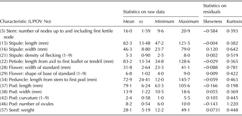
The approach developed in the current study was exemplified using a data set from UK field pea field distinctness trials from 1995 to 2013. The semi-leafless group of varieties was considered. The location of the trials was at Science and Advice for Scottish Agriculture (SASA), just west of Edinburgh (55°55′N, 3°21′W, 60 m a.s.l.). Each trial had two replicates and between 139 and 290 varieties. Thirteen quantitative characteristics were considered (Table 1). Only those varieties with 6 or more years of data were retained for this study; this left 222 varieties.
Characteristics considered in example data set with statistics. Residuals were calculated from a mixed model analysis with random effect year and fixed effect variety. Characteristics from UPOV guideline (Anon 2014b)
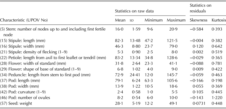
UPOV, International Union for the protection of new varieties of plants.
The combined-over-year distinctness criterion
The COYD criterion takes variety trial means for the years in which the candidate variety has been tested and applies an analysis of variance. Only varieties tested in all these years are included so the data set is balanced. The analysis of variance includes terms for year and variety effects. Using variety means over years and the least significant difference (LSD) between pairs of varieties at a set significance level, the COYD method compares the candidate with each reference variety to see whether the differences exceed the LSD.
The LSD is found using the formula:
 $${\rm LSD} = {t_{1 - {\,p \over 2},v}}\sqrt {{{2{s^2}} \over n}} $$
where t 1−p/2,v denotes the 1 − p/2 quantile of Student's t-distribution with v degrees of freedom, n is the number of years (2 or 3), s 2 is the residual variance for the COYD analysis of variance and p is the probability level set for significance. In the case of the UK field pea DUS tests, p is set at 0·02. The degrees of freedom, v, are given by (n-1) times the number of varieties less one. From here on, the approach is developed for COYD decisions based on 2 years of trials for the sake of simplicity; it would be straightforward to adapt it for 3-year decisions.
Mean measurements, x ij , are made for the characteristic of interest for each variety, i, and year, j. Taking two varieties in particular, A and B, then let the difference d j in year j, be given by d j = x Aj − x Bj Also let the COYD difference after 2 years, labelled 1 and 2, be given by D = (d 1 + d 2)/2. The COYD criterion says that variety A and variety B should be considered distinct if
 $$\left \vert {{{{d_1} + {d_2}} \over {2s}}} \right \vert \ge {t_{1 - {\,p \over 2},v}}$$
Guidance from the International Union for the Protection of New Varieties of Plants (UPOV; Anon 2014a ) describes COYD in greater detail.
An initial approach
The basis of the approach is to predict COYD decisions based on the data from the first year's trial combined with data from historical trials. The basic data considered here are the variety means in each year. Initially a number of assumptions about the data were made to allow the method to be set up in a relatively straightforward way. It was assumed that these were independent and normally distributed, and that their variances were the same in each year and for each variety and equal to σ 2. It was assumed the historical data set was large, with many varieties and years and that d j are independent and identically distributed over different years, being normally distributed with mean θ and variance 2σ 2.
It was required to estimate the probability p D that A and B would be considered distinct after 2 years of tests, given the first year's result, d 1 , and the historical data, X , i.e.
 $${\,p_D} = {\rm Pr}\left( {\left \vert {{{{d_1} + {d_2}} \over {2{s_{^\ast}}}}} \right \vert \ge {t_{1 - {\,p \over 2},{v_{^\ast}}}} \vert {d_1},{\bi \underline{X}}} \right)$$
where the degrees of freedom, v
*, the second year difference, d
2 and the 2-year residual variance,
 $s_{\ast}^2 $
are all unknown. Using this equation, tables for threshold values of d
1 can be developed for different values of p
D
.
Conditional on d 1 and σ being known, the predictive distribution of d 2 is normal with mean d 1 and variance 2σ2. If, however, σ is unknown, then the predictive distribution is Student's t-distribution (Bernardo & Smith Reference Bernardo and Smith2000) but large degrees of freedom should mean that the normal distribution is a good approximation.
Thus D = (d
1 + d
2)/2 has a normal distribution with mean d
1 and variance σ2/2. Also
 ${v_{\ast}}s_{\ast}^2 /{\sigma ^2}$
is chi-squared distributed with v
* degrees of freedom. So
 $\sqrt 2 D/{s_{\ast}}$
has a non-central t -distribution with v
* degrees of freedom and non-centrality parameter
 $\; \sqrt 2 {d_1}/\sigma $
.
If v
* is sufficiently large then D/s
* is approximately normal with mean d
1/σ and variance ½. It is then straightforward to calculate tables. Since the lower probability is very small, the threshold for d
1 for a particular value of p
D
is given by
 $\sigma \left( {{{\rm \Phi} ^{ - 1}}\left( {1 - p{\rm /2}} \right) + 1/\sqrt 2 \;{{\rm \Phi} ^{ - 1}}\left( {{p_D}} \right)} \right)$
.
The key assumptions made above were that the (residual) data are normal and that the variance is homogeneous, not depending on variety or year. Examining the effects of skewness or excess kurtosis, it was found that levels seen in the example data set (Table 1) would generally have little effect on the effectiveness of the proposed approach (Nevison & Roberts Reference Nevison and Roberts2011). Where levels of skewness or kurtosis for a characteristic would be high enough to be problematic, this might be managed by transformation or simply not considering that characteristic at this early stage.
Variance homogeneity was examined using linear mixed models with either a single residual variance or individual residual variances for years or varieties. Variety was treated as a fixed effect and year as a random effect. So
 $${x_{ij}} = \mu + {y_j} + {w_i} + {e_{ij}},$$
where μ is a constant, y
j
are random effect for years such that
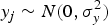 $y_j \sim N(0,{\sigma}_y^2)$
,
w
i
are fixed effects for variety and e
ij
is a random error term such that
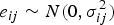 $e_{ij} \sim N(0,{\sigma}_{ij}^2)$
. In the case of homogeneity σ
ij
= σ, for yearly heterogeneity σ
ij
= σ
j
, and for varietal heterogeneity σ
ij
= σ
i
.
The importance of yearly or varietal heterogeneity was assessed by comparison of deviances relative to change in degrees of freedom. To assess the degree of heterogeneity, a reduced chi-squared statistic was calculated, being the difference in deviance between the heterogeneous and homogeneous models divided by the difference in degrees of freedom. This statistic gives a measure for the level of evidence for heterogeneity that is independent of the associated degrees of freedom. A value near to one for this statistic indicates relatively little evidence for heterogeneity whereas larger values indicate greater heterogeneity. Note that the degrees of freedom for this test were 18 for years (17 for characteristic 57) and 221 for varieties (210 for characteristic 57). Calculations were carried out with GenStat (VSN International 2012).
Extending the approach to deal with heterogeneity
It was clear that the initial approach laid out above would be inappropriate in the presence of variance heterogeneity. In particular, year-to-year heterogeneity seemed to be common (see results). So the approach was extended to incorporate year-to-year heterogeneity, estimated from the historical data.
Rather than σ
2 being treated as constant, it was modelled through an inverse gamma distribution. So the precision λ = 1/σ
2 has a gamma distribution with shape α and rate β. Given a large historical data set (large numbers of varieties in each year), the residual variance can be estimated in each year using the linear mixed model for yearly heterogeneity as described above. So variety was treated as a fixed effect, year as a random effect and the model had individual residual variances for each year. Let n be the number of years in the historical data and
 $S_j^2 $
be the estimated residual variance in year j. Maximum likelihood estimates for the gamma distribution parameters,
 $\hat \alpha $
and
 $\hat \beta $
, can be derived from the
 $1/S_j^2 $
by iteration (Choi & Wette Reference Choi and Wette1969; Minka Reference Minka2002). Several statistical software packages have facilities for estimating gamma distribution parameters; for example R (R Core Team 2014) has the ‘fitdistr’ function in the MASS library. Note that
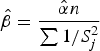 ${\hat \beta} = \displaystyle{{{\hat \alpha}n} \over {\mathop \sum {1/S_j^2}}}$
.
As for the homogeneous case, it was necessary to derive a distribution for the ratio D/s *. No analytic solution was found, so an approximation was developed as follows.
If λ is gamma distributed, then
 $${v_{^\ast}}s_{^\ast}^2 \; \vert \; \lambda = \displaystyle{1 \over {{\sigma ^2}}}\; \; \; \sim \; \; Ga\left( {\displaystyle{1 \over 2}{v_{^\ast}},\displaystyle{1 \over 2}\lambda} \right){\rm, so}$$
 $$Pr\left( {{v_{^\ast}}s_{^\ast}^2 {\rm \vert} {\bi \underline{X}}} \right) = \;\int_0^\infty {Pr\left( {{v_{^\ast}}s_{^\ast}^2 {\rm \vert} \lambda} \right)Pr\left( {\lambda {\rm \vert} {\bi \underline{X}}} \right)d\lambda} \hbox{, and thus}$$
 $${v_{^\ast}}s_{^\ast}^2 \vert \; {\bi \underline{X}} \; \sim \; Gg\left( {\hat \alpha, \displaystyle{{2\hat \alpha n} \over {\mathop \sum \nolimits {1/S_j^2}}}, \displaystyle{1 \over 2}{v_{^\ast}}} \right){\rm,} $$
where Gg is the Gamma–Gamma distribution (Bernardo & Smith Reference Bernardo and Smith2000).
By compounding a normal distribution with unknown precision with a gamma distribution over the precision, it was found that
 $\sqrt 2 D\; $
has a non-standardized Student's t-distribution, so that
 $\sqrt 2 D = \sqrt 2 {d_1} + \sigma {t_{2\hat \alpha}} $
, where
 ${t_{2\hat \alpha}} $
has Student's t-distribution on
 $2\hat \alpha $
degrees of freedom.
From the above, expectations and variances can be inferred, so
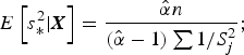 $$E\left[ {s_{\ast}^2 \vert {\bi X}} \right] = \displaystyle{{{\hat \alpha }n} \over {({\hat \alpha} - 1)\mathop \sum \nolimits{1/S_j^2}}};$$
 $$V\left[ {s_{\ast}^2 \vert {\bi X}} \right] = \displaystyle{{(v_{\ast} + 2{\hat \alpha} - 2)} \over {v_{\ast}({\hat \alpha} - 2)({\hat \alpha} - 1)^2}}\left(\displaystyle{{{\hat \alpha} n} \over {\mathop \sum \nolimits {1/S_j^2}}} \right)^2,$$
 $$E\left[ D \right] = {d_1}\; {\rm and}\; V\left[ D \right] = {1 \over 2}{n \over {\mathop \sum \nolimits {1/S_j^2}}} {{\hat \alpha} \over {\hat \alpha - 1}}$$
Through the second-order Taylor expansion, an approximation for the expectation of the required ratio was derived:
 $$E\left[ {\displaystyle{D \over {{s_{^\ast}}}}} \right] \approx \left( {1 + \displaystyle{3 \over 8}\displaystyle{{{v_{^\ast}} + 2\hat \alpha - 2} \over {{v_{^\ast}}\left( {\hat \alpha - 2} \right)}}} \right){d_1}\sqrt {\displaystyle{{\hat \alpha - 1} \over {\hat \alpha}} \displaystyle{{\mathop \sum \nolimits {1/S_j^2} \over n}}}$$
and through the first-order Taylor expansion, an approximation for its variance:
 $$V\left[ {\displaystyle{D \over {{s_{^\ast}}}}} \right] \approx \; \displaystyle{1 \over 2}\left( {1 + \displaystyle{{d_1^2} \over 2}\displaystyle{{\left( {\hat \alpha - 1} \right)} \over {\hat \alpha}} \displaystyle{{\mathop \sum \nolimits {1/S_j^2}} \over n}\displaystyle{{\left( {{v_{^\ast}} + 2\hat \alpha - 2} \right)} \over {{v_{^\ast}}\left( {\hat \alpha - 2} \right)}}} \right)$$
The degree to which the distribution of D/s * could be approximated by a normal distribution or a non-standardized Student's t-distribution with the required expectation and variance was evaluated though simulation (see below).
Using a normal distribution, an approximate threshold for d
1 for a set p
D
is given by
 $ (- B + \sqrt {{B^2} - 4AC} )/2A$
, where
 $$A = {K^2} - M{{\rm \Phi} ^{ - 1}}{({\,p_D})^2}$$
 $$B = - 2K{{\rm \Phi} ^{ - 1}}(1 - \displaystyle{\,p \over 2})$$
 $$C = {\left[ {{{\rm \Phi} ^{ - 1}}(1 - \displaystyle{\,p \over 2})} \right]^2} - L{{\rm \Phi} ^{ - 1}}{({\,p_D})^2}$$
 $$K = \left( {1 + \displaystyle{3 \over 8}\displaystyle{{{v_{^\ast}} + 2\hat \alpha - 2} \over {{v_{^\ast}}\left( {\hat \alpha - 2} \right)}}} \right)\sqrt {\displaystyle{{\hat \alpha - 1} \over {\hat \alpha}} \displaystyle{{\mathop \sum \nolimits {1/S_j^2}} \over n}} $$
L = 1/2 and
 $$M = \displaystyle{1 \over 4}\displaystyle{{\left( {\hat \alpha - 1} \right)} \over {\hat \alpha}} \displaystyle{{\mathop \sum \nolimits {1/S_j^2}} \over n}\displaystyle{{\left( {{v_{^\ast}} + 2\hat \alpha - 2} \right)} \over {{v_{^\ast}}\left( {\hat \alpha - 2} \right)}}$$
Note that if A is negative, the threshold is nonsensical. This may happen when the level of yearly heterogeneity is high and the required p D value is high. The threshold is also sensitive to the degrees of freedom, v *, especially when the level of heterogeneity is high, at least for larger values of p D (e.g. 0·999). The threshold decreases as v * increases. Given that v * is not known in advance, it would be best to choose a conservative value for v * based on experience. In the example data set, residual degrees of freedom for 2-year COYD analyses varied between 51 and 171.
Evaluation of method by simulation
Simulation was used to evaluate both the approximations made in the derivation of the threshold formula and the effect of deviations from the inverse gamma distribution assumed over the yearly residual variances.
Simulated predictions were made of the decisions made and of the ratio D/s * based on:
-
• the first year difference d 1 being set at the calculated threshold based on a particular value of p D . Thresholds were calculated for each of the characteristics in the example data set (a selection is shown here).
-
• a range of values for p D . Here values of 0·99, 0·95 and 0·90 are shown.
-
• the simulated distribution of the unknown second year difference d 2 being normal with mean d 1 and variance 2σ 2.
-
• values of s * being simulated from a gamma distribution with shape v */2 and rate v * λ/2.
-
• the precision parameter λ = 1/σ 2 being simulated either as being constant over years (homogeneity), gamma distributed (heterogeneity), log-normal distributed or Weibull distributed. The inclusion of the latter two distributions was to evaluate the calculations for sensitivity to deviations from the gamma distribution assumed. The parameters of these distributions were estimated for each of the characteristics in the example data set (a selection is shown here).
-
• the unknown degrees of freedom v * being set at 50.
-
• a simulation sample of 10 000 000.
The shape of the distribution of D/s * found by simulation was compared with normal and Student's t-distributions with the approximate mean and variance as indicated above. The probability of distinctness, p D , was also calculated by simulation and compared with the applied values.
Evaluation of method on the example data set
The UK field pea data set was used to evaluate the performance of the calculated thresholds. First-year decisions were compared with COYD decisions in consecutive pairs of years (1995/96, 1996/97, 1997/98 etc.) for each characteristic. The false positive rate is the proportion of times for each characteristic that the first-year threshold indicated a variety would be distinct from another variety when the subsequent COYD decision was non-distinct. Conversely the false negative rate is the proportion of times that the first-year decision was non-distinct when the COYD decision was distinct. The rate of false positives indicates the downside of taking early decisions – that sometimes a variety might be declared distinct when it might later be found non-distinct. The rate of false positives is of course lower for higher thresholds. The false negative rate gives an indication of how useful the threshold might be in practice; lower rates indicating that more pairs of varieties would be found distinct after the first year. For these comparisons, v * was set at 50 to give conservative thresholds given experience of historic values for v.
RESULTS
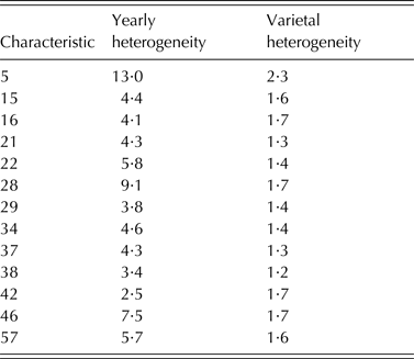
Table 2 shows the levels of heterogeneity in the field pea data. Although all cases showed evidence for some level of heterogeneity, the levels were generally much more notable for yearly heterogeneity than varietal heterogeneity. Levels of yearly heterogeneity varied considerably according to characteristic, with characteristic 5 showing the greatest degree of heterogeneity and characteristic 42 the least.
Levels of yearly and varietal heterogeneity, as assessed by mixed models with random effect year, fixed effect variety and residuals varying according to year or variety (using a diagonal variance structure)
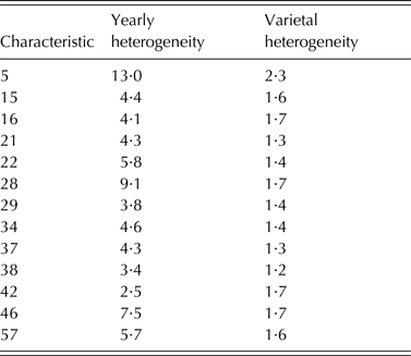
The level of heterogeneity is indicated by the reduced chi-squared statistic from the comparison of deviances. All cases showed significant better fits than the homogeneous model at the 0·01 level except for varietal heterogeneity for characteristic 38 (P-value 0·02).
Simulations showed that the approximate distributions of the ratio, D/s *, slightly overestimated the expectation and variance at least for high levels of yearly heterogeneity. Whilst the postulated normal and Student's t-distributions are symmetric, the simulations revealed that the actual distribution of the ratio has a small degree of positive skewness (in the order of 0·2). The levels of kurtosis of the distribution of the ratio are much smaller than for Student's t-distribution but are not quite zero. Thus the normal distribution was thought to be the better choice, recognizing the limitations of this approximation.
Figure 1 shows the performance of both the homogeneous and heterogeneous threshold methods. This assessment was based on the simulations using gamma, log-normal and Weibull distributions for four characteristics. These characteristics were chosen to represent different levels of yearly heterogeneity seen in Table 2. The performance was indicated by the difference between the estimate of p D found through simulation and the actual value of p D that the threshold was based on. This assessment was designed to indicate the degree to which the approximation works (based on the normal distribution) and how well the calculated thresholds work with heterogeneous data simulated from different distributions.
Difference between p D value recovered by simulation and the set p D value for different levels of heterogeneity exemplified by four characteristics and assuming the heterogeneity can be modelled by a gamma distribution, a log-normal distribution or a Weibull distribution. The method accommodating yearly heterogeneity is indicated by circles and assuming homogeneity by triangles. The horizontal line indicates no difference.

The results showed that even for characteristic 42, which had the least yearly heterogeneity, the threshold method based on heterogeneity outperformed the simpler one assuming homogeneity. As the degree of yearly heterogeneity increased so the advantage in accommodating it increased. Comparing the simulations under different distributions, overall the Weibull distribution produced more negative differences than the log-normal or gamma distributions. With the gamma and log-normal distributions, the difference for the threshold based on yearly heterogeneity was generally positive, indicating that the threshold was bigger than it needed to be. The difference was smaller for a p D of 0·9 than for 0·99, at least relative to error rate (1- p D ). When p D was 0·9, the resulting threshold had probabilities ranging from 0·9030 for the least heterogeneous characteristic, 42, to 0·8960 for characteristic 5, the most heterogeneous. When p D was 0·99, the resulting probabilities ranged from 0·9948 for characteristic 42 to 0·99967 for characteristic 5.
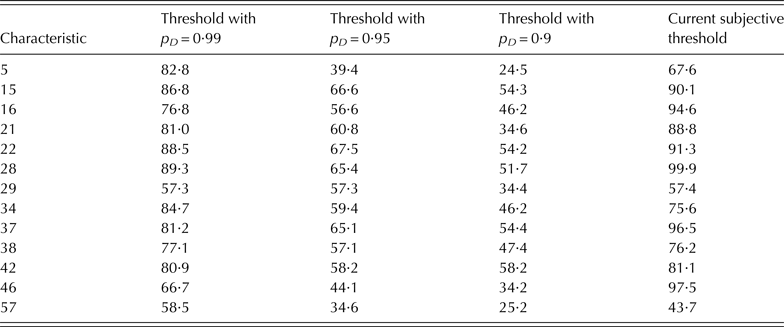
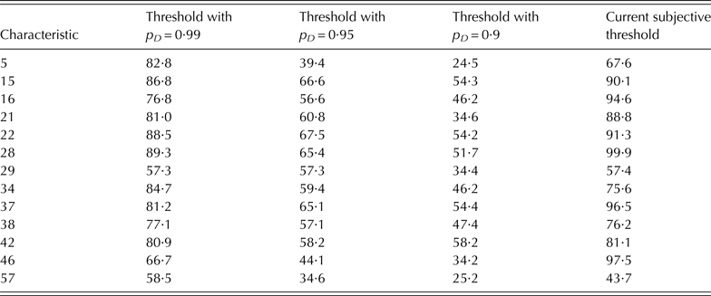
For the evaluation of performance on the field pea data set, Table 3 shows the rates of false positives and Table 4 shows the rates of false negatives. These rates were compared between three levels of p D for the calculated threshold allowing for yearly heterogeneity and the existing expert-defined threshold. The performance varied between characteristics. Some were clearly more useful, e.g. 29, 46 and 57 have low false negative rates even with p D being 0·99. Overall these results should be interpreted with care since typically reference varieties that were clearly distinct from the candidate in at least 1 characteristic after the first year may have been removed from further comparisons. However the effect of this selection would be to give a pessimistic view of the performance of the calculated thresholds.
Percentage of times that the first-year threshold allowing for yearly heterogeneity indicated a variety would be distinct from another variety when the subsequent COYD decision was non-distinct in the field pea data set (false positive)
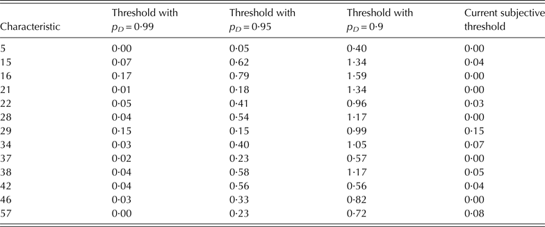
COYD, combined-over-years distinctness criterion.
Percentage of times that the first-year threshold allowing for yearly heterogeneity indicated a candidate variety would be non-distinct from another variety when the subsequent COYD decision was distinct in the field pea data set (false negative)
COYD, combined-over-years distinctness criterion.
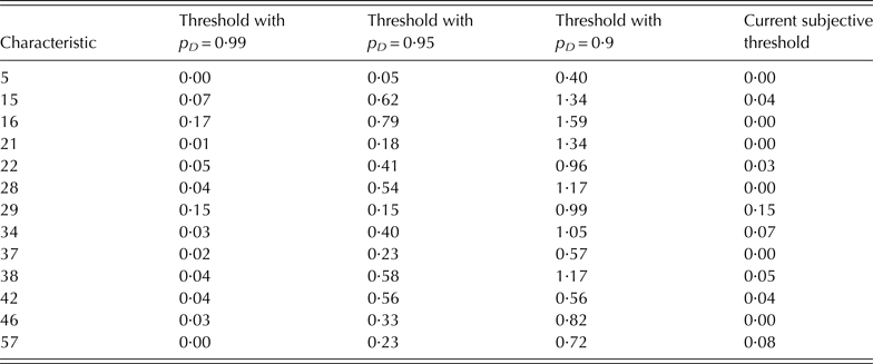
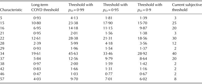
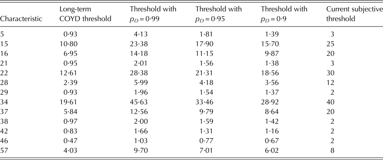
Table 5 shows the calculated thresholds for the pea example data set. The table also shows long-term COYD 2-year thresholds with p being 0·02, based on the residual variance from a mixed model analysis of the 19-year field pea data set, with year being treated as random effect and variety being treated as a fixed effect and assuming homogeneous residual variance. Note that the actual COYD thresholds varied between pairs of years in this data-set; the long-term COYD threshold represents an average threshold. Comparison with these ‘typical’ COYD thresholds demonstrates how much larger the 1-year thresholds need to be. Alongside these thresholds are the existing expert-defined thresholds currently used in the UK for field pea. The calculated thresholds with p D being 0·9 or 0·95 were all lower than the current tolerances, and with p D at 0·99 the calculated thresholds were lower for 9 out of 13 characteristics. It was noted previously that the thresholds may be sensitive to the value of the unknown degrees of freedom v *, especially when p D is high. In this data set with p D being 0·99, the calculated thresholds were 2·8% higher on average when v * was 50 compared with v * being 100. When p D was 0·95 the mean increase was 0·98%.
Post-first year thresholds allowing for yearly heterogeneity and based on v* having a value of 50. For comparison, the tolerances currently used in the UK for field pea are included alongside the long-term 2% COYD 2-year thresholds
COYD, combined-over-years distinctness criterion.
DISCUSSION
A method has been proposed to predict COYD distinctness decisions based on the first year of results. It has been adapted to ensure that it will accommodate yearly heterogeneity in the variety-by-year variance, a commonly occurring aspect of distinctness trial data. The method is straightforward to implement, given access to software that allows estimation of diagonal variance structures in mixed models (e.g. GenStat, ASReml).
The method uses approximations. The quality of the approximation was examined by simulation and was found to be suitable for the purpose intended. The approximation is better with the probability of distinctness set at 0·9 rather than 0·99. At 0·99 the threshold is larger than required so at least the approximation is conservative. It would be possible to produce exact thresholds using simulation-based calculations. However this would be significantly more difficult for the intended users to implement.
The thresholds are also more sensitive to the value of the unknown degrees of freedom, v *,when the probability of distinctness is set at 0·99 than when it is 0·95. So it is recommended that a conservative value of v * should be set based on experience, especially if a higher probability of distinctness is to be used.
The method described in the current paper also makes an assumption that the yearly heterogeneity can be satisfactorily modelled using a gamma distribution. It would not be possible to find a data set large enough to check the fit to this assumption. However the performance of the threshold under alternative distributional assumptions does give some assurance that the method is reasonably robust.
The approach has been applied to an example data set based on 19 years of field pea distinctness trials. First-year decisions were compared with 2-year COYD decisions. Care is needed in interpreting these results since typically reference varieties that were clearly distinct from the candidate in at least one characteristic after the first year may have been removed from further comparisons. The DUS crop expert is likely to want to achieve a very low false positive rate but with some potential to reduce the number of varieties to be compared in the second year. There is the obvious question as to how high a false positive rate is acceptable. In the case of the UK, a conservative approach will be taken. The calculated thresholds with the distinctness probability set at 0·99 had reasonable levels of false positives and false negatives. It is planned to move to these thresholds even when the threshold increases, except for characteristics 21, 29 and 42, which are scored on an integer scale from 1 to 9.
The COYD prediction method could be integrated with existing systems or tools for identifying reference varieties that are clearly distinct from the candidate after the first year. A particular tool documented in UPOV guidance documents is known as GAIA (Anon 2014a ): it uses expert opinion to guide derivation of threshold distances and weights over characteristics. The method proposed here should be capable of deriving more effective and verifiable thresholds for quantitative characteristics.
This method is likely to be most effective in reducing trial sizes when the reference collection is large but the number of candidates is fairly small. Combining the method with the use of grouping characteristics can increase its effectiveness further.
Another use of the method might be to give guidance to applicants on the likelihood that their variety might be found non-distinct. The method can be used to give probabilities of distinctness for each characteristic and any pair of varieties under test after the first year. For a candidate, it would be necessary to combine these, over the characteristic to find the overall probability that would be found distinct from a particular reference variety. The applicant might be advised if this probability was low. This idea will be the subject of future work. One issue to be dealt with is how to combine the probabilities given possible associations between characteristics.
The construction of the approach has been influenced by Bayesian prediction techniques and to some it may qualify as being Bayesian. However no explicit priors are used and the estimation of the parameters of the gamma distribution is frequentist. The Bayesian approach could be taken further, particularly if the prediction were to be based on the technical questionnaire submitted by the applicant prior to the first year's trial. The information provided in the questionnaire about the characteristics of candidate could be combined with the knowledge of the crop expert to produce prior predictive distributions.
Other methods for reducing the size of trials include cyclic planting, grouping characteristics and molecular markers. Cyclic planting (Camlin et al. Reference Camlin, Watson, Waters and Weatherup2001) is mostly used for 3-year distinctness tests. Reference varieties are planted in 2 out of 3 years. It cannot be used in combination with other methods for reducing the trial size so the reduction in the number of reference varieties to be planted is limited to 33%. The potential for using molecular markers for distinctness assessment has been discussed much in recent years; UPOV has a working group on this topic and produced a guidance document (Anon 2013). Because of the primacy of phenotypic characteristics for DUS assessment, the use of molecular characteristics is restricted. Essentially it must be shown that decisions using molecular markers would be consistent with those using the agreed set of phenotypic characteristics. To date, most success has been with markers that link closely to individual phenotypic characteristics such as disease resistance (Arens et al. Reference Arens, Mansilla, Deinum, Cavellini, Moretti, Rolland, van der Schoot, Calvache, Ponz, Collonnier, Mathis, Smilde, Caranta and Vosman2010). Another approach has been to correlate genetic distance to phenotypic distance but the success of this has been more mixed so far (Jones et al. Reference Jones, Norris, Smith, Cockram, Lee, O'Sullivan and Mackay2013).
This work was funded by the Scottish Government.